geometrical and topological approaches … · section 6 presents the above mentioned application...

ITcon Vol. 14 (2009), Paul & Borrmann, pg. 705

www.itcon.org - Journal of Information Technology in Construction - ISSN 1874-4753

GEOMETRICAL AND TOPOLOGICAL APPROACHES IN BUILDING

INFORMATION MODELLING

PUBLISHED: October 2009 at http://www.itcon.org/2009/46 EDITORS: Rezgui Y, Zarli A, Hopfe C J

Norbert Paul

Computation in Engineering, Technische Universität München, Germany

André Borrmann

Computation in Engineering, Technische Universität München, Germany

SUMMARY: This paper presents concepts for dealing with topological information in building information

models. On the one hand, it shows how to derive topological relationships from “traditional” building models

consisting of unconnected B-Rep bodies by means of geometric processing algorithms. On the other hand, it

discusses the capabilities of building modelling based on topological concepts. This approach combines

relational database design principles with algebraic and point set topology and shows how complexes—in

particular cw-complexes—and topological spaces can be stored in relational databases. To make complexes

suitable for building modelling it is necessary to extend them by geometric properties. Finally, the paper depicts

an advantageous application of cell-complex-based modelling: the separation of the building model into an

abstract specification of building entities (sketch), a collection of possible concrete realizations of such sketch

entities (details), and a specification of the details used by sketch entities. Then a working drawing results from

the spatial version of the relational operator inner equi-join, the so-called fibre product.

The first section of this paper introduces into the problem and into current modelling concepts. Section 2

discusses geometry-based modelling whereas the following sections present the topological approach. First,

Section 3 takes a topological view on buildings and then Section 4 discusses the corresponding data models. At

Section 5 geometry is re-introduced. Section 6 presents the above mentioned application and, together with the

subsequent conclusion, advocates the topological viewpoint.

KEYWORDS: BIM, Topological approach

REFERENCE: Paul N, Borrmann A (2009) Geometrical and topological approaches in building information

modelling, Special Issue Building Information Modeling Applications, Challenges and Future Directions,

Journal of Information Technology in Construction (ITcon), Vol. 14, pg. 705-723, http://www.itcon.org/2009/46

COPYRIGHT: © 2009 The authors. This is an open access article distributed under the terms of the Creative

Commons Attribution 3.0 unported (http://creativecommons.org/licenses/by/3.0/), which

permits unrestricted use, distribution, and reproduction in any medium, provided the

original work is properly cited.

1 INTRODUCTION

In building and construction planning one often has to deal with information along the lines of “Which elements

are connected together?” or “How are different parts separated?”. In floor plan layout, for example, such

connectivity information can describe the accessibility of rooms within an office or an apartment as well as

describing which room lets in daylight, as this calls for connectivity between the room in question and the area

outside the building. Structural analysis also requires information on the structural elements that are joined

together and the joints employed in the process.


Such connectivity information is a topological property of a building, and we will later see, that it may even be

called the topology of a building. A topological space can informally be described as a set of elements together

with a specification of which element is “close to” some other elements. Then a mapping from one such space to

another is called continuous, if the image of a point “close to”' some set remains “close to” the image set and is

accordingly not torn off the latter. Typical examples of such a continuous mapping are the affine transformations

in the Euclidean space with its so-called natural topology. If such a continuous mapping has a continuous

inverse, this mapping is called topological isomorphism or homeomorphism, for short. A typical

homeomorphism is an invertible affine transformation such as translation, rotation or shear. Note that under a

homeomorphism the image of an element “not close to” some other elements is “not close to” their image either.

The original space and the image space are then indistinguishable with respect to this “closeness” relation and is

hence called topologically equivalent or homeomorphic.

Topological relationships between building components define the basic functionality of the building (e.g. its

structural system, the connectivity of rooms) and knowledge about them can be used for a wide number of

analytical tasks (evacuation simulation, building performance analysis, etc.). A dividing wall between two

interior rooms, for example, has different thermal requirements than a dividing wall between an interior room

and the space outside the building. So there is a good reason for topological properties to show up in building

product models and, indeed, every noteworthy such model like RATAS, COMBINE or IFC deals with this kind

of information (Björk 1992; Dubois et al. 1995; Adachi et al. 2003). It is, however, difficult to access

topological information in building product models as, generally speaking, many different approaches towards

modelling topology coexist within one model.

With this heterogeneity of data types it is difficult to develop applications which have to navigate within this

space of interconnected entities in order to perform thermal or structural analysis or other aspects of the

building's performance (Romberg et al. 2004; van Treeck and Rank 2007). There is yet another topological

structure within a building product model: the data structures used to describe the geometric representation of

each building element. These structures are often defined by boundary representation (b-rep) techniques using

primitive geometric entities like point, edge and face together with connectivity information between these

primitives, hence a topology for them, too. This connectivity information, however, is only local to the specific

geometric entity, which is therefore isolated from other entities in terms of b-rep connectivity. So topological

relationships between building elements must either be derived from their geometric shape or stored explicitly in

the building model. The realization of these diverging approaches is discussed in the following sections.

2 RELATED WORK

Using Algebraic Topology for modelling buildings has already been proposed by a number of researchers, e.g.

in (Huhnt and Gielsdorf 2006; Clemen and Gielsdorf 2008; Krämer and Huhnt 2009). However, the potential of

this formal approach with respect to concrete applications has not been fully developed so far. In the context of

3D Geographic Information Systems (GIS), simplicial complexes have been employed to model soil layers, for

example (Breunig et al. 1994; Pilouk 1996; Shi et al. 2003). Simplexes are a generalization of closed, filled

triangles and are often used instead of cells to set up a so-called simplicial complex.

The potential benefits of using GI systems—in particular its topological functionality—for the analysis of

dynamical processes in buildings are discussed in (Ozel, 2000). Ozel states that, even if component-oriented

CAD systems provide sophisticated functionality for geometric modelling, they normally lack comprehensive

spatial analysis capabilities. For this reason, Ozel stores floor plans of buildings in a GIS database in order to use

its 2D spatial analysis facilities. Ozel underlines the fact that 3D spatial analysis would be a much more

powerful tool for analyzing processes in buildings. It is noteworthy, that GIS, being originally intended for

geographic modelling, is flexible enough to be used in such an unusual manner. This flexibility can surely be

attributed to the strict separation of the spatial functionality and the possibilities to model non-spatial data which


is typical for the GIS community. Such a “generic spatial modelling” approach is also advocated by (Mäntylä

1988).

The intersection concept to define topological relationships between sets was first applied to intervals in one-

dimensional space (Pullar, 1988) and later extended to cover also relations between simple regions in 2

(Egenhofer & Franzosa, 1991). Its so-called dimensional extension was developed by (Clementini & Di Felice,

1995) and is currently the OGC standard for topological relationships (OpenGIS Consortium, 1999).

3 THE GEOMETRICAL APPROACH

What we refer to here as the “geometrical approach” involves building models which considers a building a

compilation of geometric objects located in 3D space. Each of these objects has a connected and compact

geometrical shape which is described using established techniques from solid modelling such as constructive

solid geometry (CSG), swept representations or the particularly interesting boundary representation (b-rep)

techniques (Mäntylä 1988). So far, our approach complies with how CAD systems and common product models

such as IFC or CIS/2 handle building geometry today. But, whereas in product models topological relationships

between geometric objects are meant to be explicitly stored, we can also derive them from the objects’ geometry

and their relative position to each other when dealing with conventional b-rep models to avoid inconsistency.

3.1 Specification

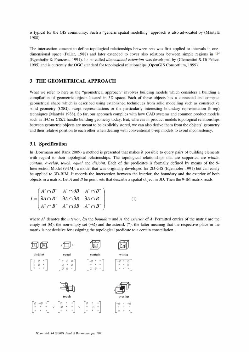
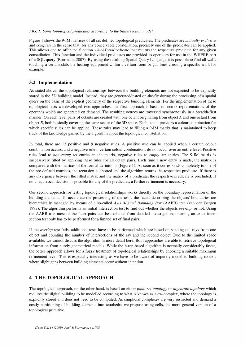
In (Borrmann and Rank 2009) a method is presented that makes it possible to query pairs of building elements

with regard to their topological relationships. The topological relationships that are supported are within,

contain, overlap, touch, equal and disjoint. Each of the predicates is formally defined by means of the 9-

Intersection Model (9-IM), a model that was originally developed for 2D-GIS (Egenhofer 1991) but can easily

be applied to 3D-BIM. It records the intersection between the interior, the boundary and the exterior of both

objects in a matrix. Let A and B be point sets that describe a spatial object in 3D. Then the 9-IM matrix reads

∩∂∩∩

∩∂∂∩∂∩∂

∩∂∩∩

=−−−−

−

−

BABABA

BABABA

BABABA

Io

o

oooo

(1)

where A° denotes the interior, ∂A the boundary and A- the exterior of A. Permitted entries of the matrix are the

empty set (Ø), the non-empty set (¬Ø) and the asterisk (*), the latter meaning that the respective place in the

matrix is not decisive for assigning the topological predicate to a certain constellation.

equal contain within

Ø Ø *

Ø Ø *

* * *

disjoint

touch

*Ø ¬Ø

* * *

* * *

* *Ø

* ¬Ø *

* * *

* *Ø

¬Ø * *

* * *

overlap

*¬Ø ¬Ø

* * *

¬Ø * *

A B

* Ø Ø

Ø * Ø

Ø Ø *

¬Ø * *

* * *

Ø Ø *

¬Ø * Ø

* * Ø

* * *

A B

A

B A

B

A

BA

B


FIG. 1: Some topological predicates according to the 9intersection model. Figure 1 shows the 9-IM matrices of all six defined topological predicates. The predicates are mutually exclusive

and complete in the sense that, for any conceivable constellation, precisely one of the predicates can be applied. This allows one to offer the function whichTopoPredicate that returns the respective predicate for any given constellation. This function and the individual predicates are provided as operators for use in the WHERE part of a SQL query (Borrmann 2007). By using the resulting Spatial Query Language it is possible to find all walls touching a certain slab, the heating equipment within a certain room or gas lines crossing a specific wall, for example.

3.2 Implementation

As stated above, the topological relationships between the building elements are not expected to be explicitly

stored in the 3D building model. Instead, they are generated/tested on-the-fly during the processing of a spatial

query on the basis of the explicit geometry of the respective building elements. For the implementation of these

topological tests we developed two approaches: the first approach is based on octree representations of the

operands which are generated on demand. The resulting octrees are traversed synchronously in a breadth-first

manner. On each level pairs of octants are created with one octant originating from object A and one octant from

object B, both basically covering the same sector of the 3D space. Each octant provides a colour combination for

which specific rules can be applied. These rules may lead to filling a 9-IM matrix that is maintained to keep

track of the knowledge gained by the algorithm about the topological constellation.

In total, there are 12 positive and 9 negative rules. A positive rule can be applied when a certain colour

combination occurs, and a negative rule if certain colour combinations do not occur over an entire level. Positive

rules lead to non-empty set entries in the matrix, negative rules to empty set entries. The 9-IM matrix is

successively filled by applying these rules for all octant pairs. Each time a new entry is made, the matrix is

compared with the matrices of the formal definitions (Figure 1). As soon as it corresponds completely to one of

the pre-defined matrices, the recursion is aborted and the algorithm returns the respective predicate. If there is

any divergence between the filled matrix and the matrix of a predicate, the respective predicate is precluded. If

no unequivocal decision is possible for any of the predicates, a further refinement is necessary.

Our second approach for testing topological relationships works directly on the boundary representation of the

building elements. To accelerate the processing of the tests, the facets describing the objects' boundaries are

hierarchically managed by means of a so-called Axis Aligned Bounding Box (AABB) tree (van den Bergen

1997). The algorithm performs an initial intersection test to find out whether the objects overlap, or not. Using

the AABB tree most of the facet pairs can be excluded from detailed investigation, meaning an exact inter-

section test only has to be performed for a limited set of final pairs.

If the overlap test fails, additional tests have to be performed which are based on sending out rays from one

object and counting the number of intersections of the ray and the second object. Due to the limited space

available, we cannot discuss the algorithm in more detail here. Both approaches are able to retrieve topological

information from purely geometrical models. While the b-rep-based algorithm is normally considerably faster,

the octree approach allows for a fuzzy treatment of topological relationships by choosing a suitable maximum

refinement level. This is especially interesting as we have to be aware of impurely modelled building models

where slight gaps between building elements occur without intention.

4 THE TOPOLOGICAL APPROACH

The topological approach, on the other hand, is based on either point set topology or algebraic topology which

requires the digital building to be modelled according to what is known as a cw-complex, where the topology is

explicitly stored and does not need to be computed. As simplicial complexes are very restricted and demand a

costly partitioning of building elements into tetrahedra we propose using cells, the more general version of a

topological primitive.


4.1 Cell complexes

We start with the observation that a building resides in the Euclidean space, in such a way that the latter is

somehow divided into a finite number of parts by the former. The difference with the topological approach is

that these parts need not be compact and that they lead to a complete partitioning of the Euclidean space: every

point in space belongs to exactly one unique building part, a room or the exterior space. Note that hierarchically

aggregated spatial objects cannot be expressed with only one such partitioning. This partitioning immediately

leads to a topology for the building elements, which is called final topology or quotient topology. This is the

topology of a building mentioned above.

4.1.1 Architectural Complexes.

From a theoretical point of view, the statement that the Euclidean space is finitely partitioned by architecture is

still too weak. We say that every building part can also be further subdivided into a finite number of cells which

set up a special case of a topological space with interesting algebraic properties. It is the so-called cw-

complex—a composition of cells frequently used in Algebraic Topology (Hatcher 2002). An n-cell (cell of

dimension n) is a topological space which is homeomorphic to the interior of an n-dimensional cube. For the

special case of n=0 we say a 0-cell is a space with exactly one point. Low dimensional n-cells are often called

topological primitives in volume modelling. A 0-cell is also called vertex, “1-cell” is a synonym for “edge”, 2-

cells are “faces” and 3-cells are also called “volumes”. Figure 2 shows the canonical cells found in a closed

cube. It is important, however, that a cell's boundary is never part of the cell.

FIG. 2: The canonical cellular decomposition of a closed 3d-cube

Now these cells can be combined to form a topological space which is called cw-complex. This is a topological

space partitioned into a set C of cells where the boundary of each cell is a union of a finite number of cells in C

of strictly lower dimension than n. We always assume C be finite.

Then for some integer number i, the set iX X⊆ , the union of iC C⊆ of cells of at most dimension i is

called i-skeleton of X. This is also a cw-complex with partitioning Ci. Each i+1-cell is also said to be attached to

the i-skeleton. Note that i may even be negative, in which case Xi=Ø.

The 0-skeleton is simply the discrete vertex set (or point cloud) and the 1-skeleton is a graph, where the edges

are attached to the vertices. Attaching faces to the 1-skeleton can be done by either filling loops or by creating

cavities and gives rise to the 2-skeleton (a sponge-like structure) which is then completed to form the 3-skeleton

by filling cavities with volumes. Theoretically, attaching a volume could also create hyper-cavities, but we will

refrain from that. Note that, if one neglects the rooms of a building, it also displays a “sponge-like structure”.

Note also that a single b-rep volume model is likewise a cw-complex.


FIG. 3: The skeletons of the canonical cw-complex of a three-dimensional closed cube, beginning with X3 on the left and ending with X0 to the right. Note that Xn = X3 for all n ≥ 3 and Xn = Ø if i is a negative integer.

4.1.2 Complex Based Modelling At the most detailed level, the building elements are cells which are basically the same objects used in b-rep

volume modelling. Only the 3-cell as a “primitive” is missing in some of these models which mostly identify a

volume with its boundary instead of providing it as a separate primitive. We attach volumes to faces instead of

such identification and will therefore model the connectivity information in a different way. Later the notion of a

cell will be relaxed and walls or slabs can be considered faces by simply disregarding their relatively small

thickness. Another important difference between the cw-complex-based representation and the boundary

representation of a building is that connecting faces between adjacent building elements are not modelled

separately but can be shared by both elements.

FIG. 4: In boundary representations connecting faces are modelled multiple times, whereas in CW-complexes they can be shared by adjacent volumes.

We will now proceed to describe a relational schema for an algebraic complex. It is a well-known fact that each

cw-complex has an associated algebraic complex of this kind, the so-called cellular chain complex (Hatcher

2002).

5 TOPOLOGICAL DATA MODELS

The formal definition of an algebraic complex has an associated relational database schema in a straightforward

manner. This schema even holds more topological information than its algebraic counterpart. Considering its

point-set topological properties we will see that this is also an efficient and lossless relational database schema

for every finite topological data.


5.1 Relational Complexes

Cw-complexes are often defined by specifying an inductive procedure of starting with the 0-skeleton X0 and

then attaching i+1-cells to the i-skeleton until the complex is finished (Hatcher 2002, p. 5).

We will repeat this inductive procedure with an example volume element, a closed unit cube of dimension 3,

and, in parallel, give a relational representation of the associated algebraic complex to illustrate the notion of a

relational complex (Paul 2007). We only present here what we call the dynamic version of a relational complex,

where all cells are stored in one single table together with an attribute to indicate the dimension.

We start with our specimen cube's vertices and establish the 0-skeleton as a relation with the schema

CELLS(id:Z , dim:Z )

with primary key {id, dim}.The coordinates of these cells set up another relation of schema

COORD(id:Z ,dim:{0}→ x,y,z:R )

We indicate the primary key by an arrow pointing from the primary key attributes to all other attributes. The

attribute COORD.dim is constantly the integer 0 and only used to establish a reference to CELLS. We call each

entry in COORD a point and each entry in CELLS with dim=0 a vertex. Each point must reference a vertex.

So by simply storing the eight vertices and points in the corresponding relations we obtain the 0-skeleton of our

specimen cube.

Now we have to paste edges to vertices. This will be done by adding records with a dim-value of 1 to the cells

table and calling these records edges or 1-cells. To be able to attach these cells to vertices we finally define our

last additional relational schema

BD(a,dimA, b,dimB → alpha:Z )

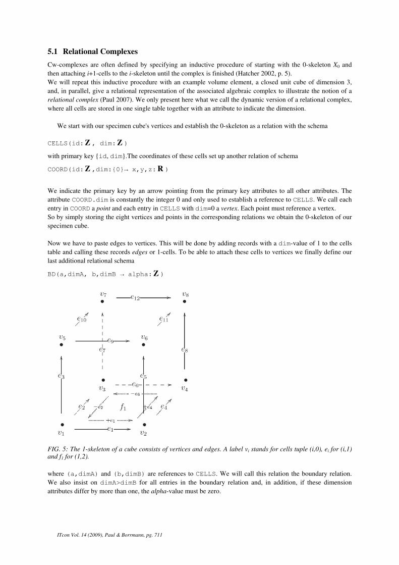
FIG. 5: The 1-skeleton of a cube consists of vertices and edges. A label vi stands for cells tuple (i,0), ei for (i,1) and f1 for (1,2).

where (a,dimA) and (b,dimB) are references to CELLS. We will call this relation the boundary relation.

We also insist on dimA>dimB for all entries in the boundary relation and, in addition, if these dimension

attributes differ by more than one, the alpha-value must be zero.


Note that BD defines a partial integer matrix D, which maps some pairs (e,v) of cells to an integer D(e,v) and is

undefined for others. To obtain a total matrix, all undefined entries can be regarded as zero entries. Each edge e

of our cube running from vertex a to vertex b will now be stored as one record (e,1) in the cells relation and two

additional records (e,1, a,0,–1) and (e,1, b,0,+1) in the boundary relation, indicating that edge e (of dimension 1)

starts at vertex a (of dimension 0) and ends in b. The orientation of each edge can be arbitrarily chosen and, in

our example, we simply let an edge run from lower id to higher id. This produces a 1-skeleton, displayed in

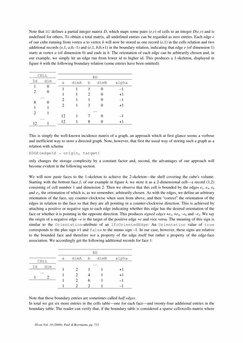
figure 4 with the following boundary relation (some entries have been omitted):

CELL

Id dim

1 0

2 0

…

8 0

1 1

2 1

…

12 1

BD

a dimA b dimB alpha

1 1 1 0 –1

1 1 2 0 +1

2 1 1 0 –1

2 1 3 0 +1

…

12 1 7 0 –1

12 1 8 0 +1

This is simply the well-known incidence matrix of a graph, an approach which at first glance seems a verbose

and inefficient way to store a directed graph. Note, however, that first the usual way of storing such a graph as a

relation with schema

EDGE(edgeId → origin, target)

only changes the storage complexity by a constant factor and, second, the advantages of our approach will

become evident in the following section.

We will now paste faces to the 1-skeleton to achieve the 2-skeleton—the shell covering the cube's volume.

Starting with the bottom face f1 of our example in figure 4, we store it as a 2-dimensional cell—a record (1,2)

consisting of cell number 1 and dimension 2. Then we observe that this cell is bounded by the edges e1, e4, e6

and e2, the orientation of which is, as we remember, arbitrarily chosen. As with the edges, we define an arbitrary

orientation of the face, say counter-clockwise when seen from above, and then “correct” the orientation of the

edges in relation to the face so that they are all pointing in a counter-clockwise direction. This is achieved by

attaching a positive or negative sign to each edge indicating whether this edge has the desired orientation of the

face or whether it is pointing in the opposite direction. This produces signed edges +e1, +e4, –e6 and –e2. We say

the origin of a negative edge –e is the target of the positive edge +e and vice versa. The meaning of this sign is

similar to the Orientation-attribute of an IfcOrientedEdge: An Orientation value of true

corresponds to the plus sign +1 and false to the minus sign –1. In our case, however, these signs are relative

to the bounded face and therefore not a property of the edge itself but rather a property of the edge-face

association. We accordingly get the following additional records for face 1:

CELL

Id dim

…

1 2

BD

a dimA b dimB alpha

…

1 2 1 1 +1

1 2 4 1 +1

1 2 6 1 –1

1 2 2 1 –1

Note that these boundary entries are sometimes called half edges.

In total we get six more entries in the cells table—one for each face—and twenty-four additional entries in the

boundary table. The reader can verify that, if the boundary table is considered a sparse cells×cells-matrix where


the rows are indexed by (a,dimA)-pairs, the column index is (b,dimB) and the entries are the associated

alpha values, then it returns a sparse zero matrix if multiplied by itself.

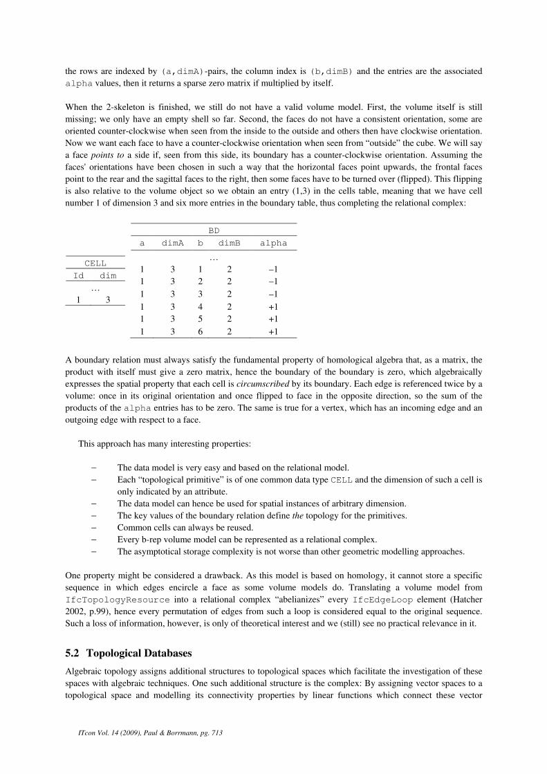
When the 2-skeleton is finished, we still do not have a valid volume model. First, the volume itself is still

missing; we only have an empty shell so far. Second, the faces do not have a consistent orientation, some are

oriented counter-clockwise when seen from the inside to the outside and others then have clockwise orientation.

Now we want each face to have a counter-clockwise orientation when seen from “outside” the cube. We will say

a face points to a side if, seen from this side, its boundary has a counter-clockwise orientation. Assuming the

faces' orientations have been chosen in such a way that the horizontal faces point upwards, the frontal faces

point to the rear and the sagittal faces to the right, then some faces have to be turned over (flipped). This flipping

is also relative to the volume object so we obtain an entry (1,3) in the cells table, meaning that we have cell

number 1 of dimension 3 and six more entries in the boundary table, thus completing the relational complex:

CELL

Id dim

…

1 3

BD

a dimA b dimB alpha

…

1 3 1 2 –1

1 3 2 2 –1

1 3 3 2 –1

1 3 4 2 +1

1 3 5 2 +1

1 3 6 2 +1

A boundary relation must always satisfy the fundamental property of homological algebra that, as a matrix, the

product with itself must give a zero matrix, hence the boundary of the boundary is zero, which algebraically

expresses the spatial property that each cell is circumscribed by its boundary. Each edge is referenced twice by a

volume: once in its original orientation and once flipped to face in the opposite direction, so the sum of the

products of the alpha entries has to be zero. The same is true for a vertex, which has an incoming edge and an

outgoing edge with respect to a face.

This approach has many interesting properties:

− The data model is very easy and based on the relational model.

− Each “topological primitive” is of one common data type CELL and the dimension of such a cell is

only indicated by an attribute.

− The data model can hence be used for spatial instances of arbitrary dimension.

− The key values of the boundary relation define the topology for the primitives.

− Common cells can always be reused.

− Every b-rep volume model can be represented as a relational complex.

− The asymptotical storage complexity is not worse than other geometric modelling approaches.

One property might be considered a drawback. As this model is based on homology, it cannot store a specific

sequence in which edges encircle a face as some volume models do. Translating a volume model from

IfcTopologyResource into a relational complex “abelianizes” every IfcEdgeLoop element (Hatcher

2002, p.99), hence every permutation of edges from such a loop is considered equal to the original sequence.

Such a loss of information, however, is only of theoretical interest and we (still) see no practical relevance in it.

5.2 Topological Databases

Algebraic topology assigns additional structures to topological spaces which facilitate the investigation of these

spaces with algebraic techniques. One such additional structure is the complex: By assigning vector spaces to a

topological space and modelling its connectivity properties by linear functions which connect these vector


spaces it is possible to investigate topological properties using linear algebra. We will now go the inverse

direction and forget the algebraic property by simply removing the alpha values from the boundary relation.

What then remains is a simple directed graph (X, R) where X denotes the cell set and R ⊆ X×X the incidence

relation: If x R y holds then element y is a boundary element of x.

For example

kitchen R kitchen-door,

means “The kitchen door is a boundary element of the kitchen”.

Before we proceed we must have a clear understanding of what is called “topology” and “topological property”.

A topology for a set X is the set TX of each subset of X, which is considered the “interior of itself”, and is then

called “open”. Every other topological property can then be expressed using these open sets.

It can easily be shown that such a relation R defines a topology TR on the set X, and therefore (X, TR) will be

called the topological space associated to (X, R). A set U is open in (X, TR) iff (meaning “if and only if”) for

every point u in U und every edge (x,u) in R which has an ending point in U the starting point x is also in U. On

the other hand, each so-called Alexandrov topological space (X, T) has such a graph (X, ≤T). The relation ≤ is

sometimes called the specialization preorder of (X, T). In particular, each finite topological space is Alexandrov.

Note that each building product model is finite too: it only consists of finitely many elements. As that relation is

a lossless encoding of the topology (Alexandrov 1937) we also call a simple directed graph a topological data

type, because we have its straightforward relational database implementation in mind. A family of topological

data types is then likewise called topological database. Note that this is an extremely simple data model

compared to all other topological modelling approaches. A relational complex hence can be considered a

topological data type by simply ignoring the alpha-values.

So far we have only provided a new name for the well-known traditional data model named “graph”. We will

now show, how topological properties and operators can be expressed using relational algebra and then, on the

other hand, propose an adaptation of these relational operators to topological databases based on the theory of

topological constructions.

5.2.1 Continuous Database Maps

First we will provide a relational version of continuous maps between topological spaces because they have

important applications: First, they are used to compare topological spaces and, in particular, to define under

which conditions two such spaces can be considered essentially equal or homeomorphic. Second, these maps

play an important role in topological constructions, which is what our topological query operators are. Just like

topological constructions every relational query operator has typical maps which link the input relations to the

resulting output relation. In topology these maps must be continuous, which gives a unique topology for each

query result.

A continuous map is a map f : X→Y, from the point sets of two topological spaces (X,TX) and (Y,TY) which

respects their topologies: Each point p ∈ X which is “close to” a set A is not torn away from the image set f[A]

by a continuous function. Hence if the mapped point f(p) is also “close to” the mapped set f[A]. Continuous

maps are denoted by

f:(X, TX)→(Y, TY).

Being “close” to a set means being an element of the set itself or an element of the set’s boundary. The precise

definitions of “interior”, “boundary”, “closure” and “exterior” can be looked up in any topology textbook.

In the special case of an Alexandrov space this relation p ∈ cl A, (read: “p is close to A”) between points and

sets is completely specified by the binary relation p ≤ q iff p ∈ cl {q} between the points—the specialization

preorder mentioned above. Hence continuity between two topological data types can be expressed by the

specialization preorders of the maps involved:


A map f : X→Y between Alexandrov spaces (X, TX) and (Y, TY) is continuous iff from a ≤ b in (X, ≤) always

follows: f(a) < f(b) in (Y, <). Here ≤ and < denote the corresponding specialization preorders.

Now that preorder is known to be reflexive (each element is “close to” itself”) and transitive (if a kitchen door

border is close to a kitchen door which itself is close to a kitchen, then that kitchen door border is close to the

kitchen, too). On the other hand we defined topological data types as (X, R), where R can be any relation on X

and need not be transitive nor reflexive. Now the specialization preorder of the associated topological space

(X, TR) is simply the transitive and reflexive closure RT* of RT, the transpose of R. Hence a map f : X→Y, from

the point sets of two topological data types (X, R) and (Y, S) is continuous between the associated topological

spaces iff f×f[R*] ⊆ S*. The map f×f is the direct product of f with itself. It is defined as f×f(a,b):=(f(a),f(b)).

Now it can be easily shown, that the transitive closure R* at the left hand side of the inclusion doesn’t have to be

computed. Hence we call a map f f : X→Y which satisfies f×f[R] ⊆ S* a continuous database map, and denote if

by f : (X, R)→(Y, S) .

It can also be shown, on the other hand, that in general the right hand side transitive closure computation S* can

not be avoided to decide continuity (Paul 2008).

5.2.2 Constructive Spatial Queries

The above mentioned spatial query language is still restricted to querying topological properties. Basing this

model on the relational model offers an interesting perspective: If one takes a relational view of topological

spaces, one might, conversely, ask how the relational operators themselves can be given a topological meaning.

Indeed, except for the outer join, every operator in relational algebra has a counterpart as a construction in point

set topology or such topological version of an operator in question can be easily constructed.

The following table gives some example relational operators and their corresponding topological constructions.

relational algebra point set topology

selection subspace

rename homeomorphism

Cartesian product product space

inner equi join fibre product

disjoint union topological sum

We will now present the basic relational query operators union, intersection, selection, projection and Cartesian

product of topological data types and present the characteristic maps between input data types (spaces) and the

resulting output space. The basic idea of topological constructions is first “linking” input and output elements by

characteristic maps. Then with the topologies given with the input data the output topology must be completed

such that all maps involved are continuous. If the output data is at the domain side of these maps and the input

topologies are located at their range, the complementary topology is called initial or induced topology.

Otherwise, as we already know, it is called final topology. In general, final topologies are easier computed than

initial topologies.

5.2.2.1 Set intersection and union

We assume two topological data types (X, R) and (Y, S) be union compatible. This means, that the relational

schemes of X and Y are equal and so are the schemes of R and S. Then there are two maps which are

characteristic for the union X∪Y: the injections

iX : X → X∪Y and iY : Y → X∪Y,

which are simply defined by iX(a) := a and iY(b) := b. Then the input topologies, defined by the relations R and S

belong to the domain sides of these maps and the query result is at the range side (the side at which the arrow

“ends”). Hence, our topology will be final, and it is simply generated by R∪S. So union of topological data types

is defined as


(X, R) ∪ (Y, S) := (X∪Y, R∪S).

We will always denote the topological version of a relational database query operator by underlining the

corresponding operator symbol from relational algebra, according to a common habit in topology where the

point set of a topological space is underlined to distinguish the entire topological space from its underlying point

set. Hence X ≠ X := (X, T).

The case of intersection X∩Y is somewhat different to union, as its characteristic maps go the inverse direction

from query result into the input data:

jX : X∩Y → X and iY : X∩Y → Y.

So our topology is located at the domain side (where the arrow “starts”) of these maps which gives an initial

topology, the computation of which is somewhat more costly: It is defined by the relation R+∩S+, the

intersection of the transitive closures of the input relations. Hence intersection of topological data types can be

defined as

(X, R) ∩ (Y, S) := (X∩Y, R+∩S+).

The computation of the transitive closures cannot be avoided in the general case (Paul 2008), which, however,

includes spaces of arbitrary dimension with no upper dimension limit and yet with no conceivable practical use.

5.2.2.2 Selection, Projection and Joins

We will now define the topological version of the most prominent relational database query operators and also

briefly describe their characteristic maps.

Selection of a relation (a table) T according to a predicate Θ, is the table σΘ(T) which consists of all records from

T which satisfy Θ. As σΘ(T) is a subset of T, the characteristic map is the inclusion i : σΘ(T)→T. The selection

σΘ(T, R) of a topological data type (T, R) therefore has an initial topology and is defined as

σΘ(T, R) := ( σΘ(T), (σΘ(T)×σΘ(T))∩R+ ),

assuming with no loss of generality, that R consists of pairs of records from T. This assumption, of course, is

unlikely to hold when T and R are relational database tables designed according to usual good design principles,

but it gives a simpler definition. In practical cases the above formula is very likely to have to be adopted to the

relational schemas of T and R. Again, the transitive closure computation is necessary in general.

Projection of a relation T to a set of attributes A is the table πA(T) which consists of the records from T stripped

off all attributes which are not mentioned in A. This operation is carried out record-by-record which gives a

characteristic map πA :T → πA(T), defining a final topology. With our previous assumption that topological data

types (T, R) violate normal forms, projection of topological data types is

πA(T, R) := ( πA(T), πA×πA(R)).

In this formula R is considered a set of pairs of entire records from T instead of only consisting of pairs of key

attribute values from T. Therefore we can simply write πA×πA(R) in our formal definition but must adopt this

expression to the actual schema of the input data in practice.


The Cartesian product A×B of two sets is the set of all pairs (a,b) where a is an element from A and b,

accordingly, is in B. The characteristic maps are the two projections π1(a,b) := a and π2(a,b) := b. In relational

algebra the attribute sets of the tables A and B must then be disjoint such that the records a and b can be

concatenated to a new record ab in order to satisfy first normal form, which we will ignore once again. The

Cartesian product of two topological data types (A, R) and (B, S) is

(A, R) ×(B, S) := ( A×B, R0⊗S ∪ R⊗S0 ).

The relation R0 is simply the identity relation on A: The set of all pairs (a,a) for all a∈A. Likewise S0 is the

identity relation on B. The product relation R⊗S of R and S is just the Cartesian product R×S, with the pairs

((a1,a2),(b1,b2)) from R×S rearranged into ((a1,b1),(a2,b2)), to consider them elements in (A×B)×(A×B). Note that

this is a special case of an initial topology which can be constructed without transitive closure computation. This

definition of the Cartesian product can be easily modified to satisfy first normal form. Then there is no

difference between R⊗S and R×S.

We will later present a topological version of the Cartesian product of two complexes, hence a counterpart of

Cartesian product in algebraic topology.

Inner joins and natural joins can now be defined by combining Cartesian product with selection. Outer joins,

however, will be disallowed in topological databases because their characteristic maps, the projections from the

join back to the input relations, are only partially defined and would return ambiguous results. On the other

hand, they are not needed, too, because it is always possible to avoid an outer join by adding a default record

which represents an “undefined” reference to each table involved.

6 GEOMETRIC PROPERTIES

In topology, the geometry of cells and cw-complexes is ignored. So it is necessary to extend the data model by

geometric properties in order to make it suitable for geometric modelling. We will now return to algebraic

topology as we are about to make use of the orientation values stored as alpha-values. If we first consider

solely planar objects with straight edges and plane surfaces, then it is sufficient to store the location of the

vertices in the COORD table because all other cells' geometries are then defined by linear interpolation. This

assumption is too restrictive for practical purposes, but the appropriate extension of the model presented here

can be discussed independently. We will now describe some basic geometric properties. In (Breunig et al. 1994)

a similar approach was presented for simplicial complexes.

Measures. Length, surface area, volume and maybe even their higher dimensional analogous are important

properties which must be derived from the given model. The surface of a planar polygonal surface f can be

computed by first triangulating the polygon and then summing up the surfaces of each such triangle. This

triangulation, however, need not cover the surface exactly. It is also possible to fix an arbitrary point p in the

supporting hyperplane and then for each edge (a,b) in the polygon's boundary compute the cross product

pa pb×uur uur

.

The sum of all such cross products is a vector, where its direction gives the face's orientation and its length is

twice the area of the face if all edges (a,b) are aligned with the orientation of the face itself. The reference point

p may even lie anywhere so the area of a face f is simply

∑∈

×=)(),(2

1)area(

fdba

bafrr

(2)


where d(f) is the set of all edges in the boundary of f. This formula, however, does not take into account that the

orientations of the edges are arbitrary. But then we can use the signs from our boundary relation and hence the

sum in the above formula can be replaced by:

β

β∈ − + ⊆

×⋅∑ ∑

( , , ) BD {( , , 1),( , , 1)} BD 2

r ur

f e e a e b

a b. (3)

The cross product a × b is first computed for the boundary points a, b of each edge e bounding f. This is then

multiplied by β, the flipping of the orientation of e relative to face f.

A similar approach enables us to compute the volume of a 3-cell in our complex. We triangulate the surface

(boundary) of the volume object and compute the volume of each cone (pyramid) atop such a triangle with an

appropriate sign indicating whether the cone's volume is attached to the outside or the inside of the triangle. A

natural choice for the cone's apex is the origin in 3

R .

( , , ) surface( )

1vol( )

3∈

= ⋅∑x y z

x y z

a b c v

x y z

a a a

v b b b

c c c

(4)

where surface(v) is a triangulation of v's boundary such that all triangles (a,b,c) have the same orientation when

viewed from the outside. Note that there is a close relationship between the cross product used to compute the

area and the determinant used here to compute the volume.

The triangulation of a face, say f1 from our example, can simply be done by fixing one boundary point p of f1

and then for each boundary edge e of f1 using the triangle (p,a,b), where e runs from a to b. If p happens to be

equal to a or b the triangle's volume is zero, and it can be left to the discretion of the implementer and his

complexity considerations whether such volume is computed and added or whether it is discarded in advance.

Hence for each face f we choose one arbitrary vertex vf and compute the triangles surface(v) as:

{ ( , , ) | ( , , ), ( , , ),

( , , ),

( , , ) }

vf fe

vf fe

vf fe

a b v v f f e

e a

e b

α α

α α

α α

− ⋅

+ ⋅

BD BD

BD

BD

Note that most of the predicate in the above set builder expression is an inner equi-join of copies of BD, hence

‘surface’ can also be generated by an SQL query. The arbitrarily chosen vf can be the one with the minimal

identifier so it can be chosen by the min-operator with a ‘group by’ clause. The flipping of orientation is

recognized by simply multiplying the corresponding alpha-value.

7 SKETCHES AND WORKING DRAWINGS

We have now presented a concept for storing an arbitrary cell complex. A building, however, is commonly

conceived as a union of building elements like doors, walls or columns which can be treated as if they were

cells. A door, for example, somehow resembles a 2-cell combining two volumes if we disregard its relatively

shallow thickness. The relational model presented above has the advantage that it is not restricted to cells and

can store arbitrary complexes. It clearly makes sense to store building elements and the spatial relationships

among them as spatial entities and not the cells they are made of because, firstly, this represents the semantics of

a building and, secondly, many such elements have repeated patterns, and the explicit storage of the cell

decomposition of, say, a frequently used joint would lead to redundancies. To avoid such redundancies a

topological version of relational decomposition and inner equi joins is needed and might also set up what can be

called a “topological design theory”. Such topological inner joins are well known and are called fibre products.


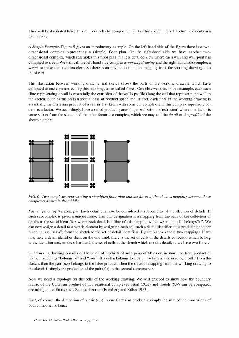
They will be illustrated here. This replaces cells by composite objects which resemble architectural elements in a

natural way.

A Simple Example. Figure 5 gives an introductory example. On the left-hand side of the figure there is a two-

dimensional complex representing a (simple) floor plan. On the right-hand side we have another two-

dimensional complex, which resembles this floor plan in a less detailed view where each wall and wall joint has

collapsed to a cell. We will call the left-hand side complex a working drawing and the right-hand side complex a

sketch to make the intention clear. So there is an obvious continuous mapping from the working drawing onto

the sketch.

The illustration between working drawing and sketch shows the parts of the working drawing which have

collapsed to one common cell by this mapping, its so-called fibres. One observes that, in this example, each such

fibre representing a wall is essentially the extrusion of the wall's profile along the cell that represents the wall in

the sketch. Such extrusion is a special case of product space and, in fact, each fibre in the working drawing is

essentially the Cartesian product of a cell in the sketch with some cw-complex, and this complex repeatedly oc-

curs as a factor. We accordingly have a set of product spaces (a generalization of extrusion) where one factor is

some subset from the sketch and the other factor is a complex, which we may call the detail or the profile of the

sketch element.

FIG. 6: Two complexes representing a simplified floor plan and the fibres of the obvious mapping between these complexes drawn in the middle.

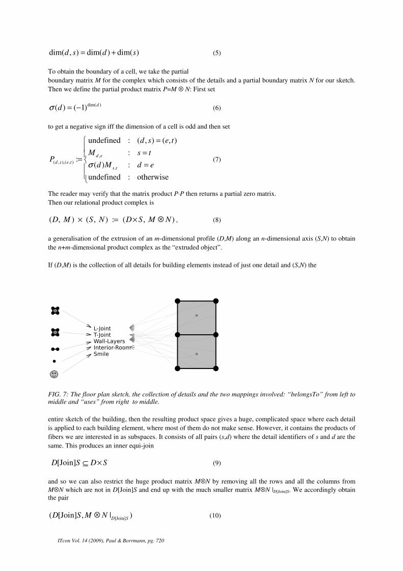
Formalization of the Example. Each detail can now be considered a subcomplex of a collection of details. If

such subcomplex is given a unique name, then this designation is a mapping from the cells of the collection of

details to the set of identifiers where each detail is a fibre of this mapping which we might call “belongsTo”. We

can now assign a detail to a sketch element by assigning each cell such a detail identifier, thus producing another

mapping, say “uses”, from the sketch to the set of detail identifiers. Figure 6 shows these two mappings. If we

now take a detail identifier then, on the one hand, there is the set of cells in the details collection which belong

to the identifier and, on the other hand, the set of cells in the sketch which use this detail, so we have two fibres.

Our working drawing consists of the union of products of such pairs of fibres or, in short, the fibre product of

the two mappings “belongsTo” and “uses”. If a cell d belongs to a detail i which is also used by a cell s from the

sketch, then the pair (d,s) belongs to the fibre product. Then the obvious mapping from the working drawing to

the sketch is simply the projection of the pair (d,s) to the second component s.

Now we need a topology for the cells of the working drawing. We will proceed to show how the boundary

matrix of the Cartesian product of two relational complexes detail (D,M) and sketch (S,N) can be computed,

according to the EILENBERG-ZILBER-theorem (Eilenberg and Zilber 1953).

First, of course, the dimension of a pair (d,s) in our Cartesian product is simply the sum of the dimensions of

both components, hence


dim( , ) dim( ) dim( )d s d s= + (5)

To obtain the boundary of a cell, we take the partial

boundary matrix M for the complex which consists of the details and a partial boundary matrix N for our sketch.

Then we define the partial product matrix P=M ⊗ N: First set

dim( )( ) ( 1) ddσ = − (6)

to get a negative sign iff the dimension of a cell is odd and then set

,

( , ),( , )

,

undefined : ( , ) ( , )

::

( ) :

undefined : otherwise

d e

d s e t

s t

d s e t

M s tP

d M d eσ

= =

= =

(7)

The reader may verify that the matrix product P·P then returns a partial zero matrix.

Then our relational product complex is

( , ) ( , ) : ( , )D M S N D S M N× = × ⊗ , (8)

a generalisation of the extrusion of an m-dimensional profile (D,M) along an n-dimensional axis (S,N) to obtain

the n+m-dimensional product complex as the “extruded object”.

If (D,M) is the collection of all details for building elements instead of just one detail and (S,N) the

FIG. 7: The floor plan sketch, the collection of details and the two mappings involved: “belongsTo” from left to middle and “uses” from right to middle.

entire sketch of the building, then the resulting product space gives a huge, complicated space where each detail

is applied to each building element, where most of them do not make sense. However, it contains the products of

fibers we are interested in as subspaces. It consists of all pairs (s,d) where the detail identifiers of s and d are the

same. This produces an inner equi-join

[Join]D S D S⊆ × (9)

and so we can also restrict the huge product matrix M⊗N by removing all the rows and all the columns from

M⊗N which are not in D[Join]S and end up with the much smaller matrix M⊗N |D[Join]S. We accordingly obtain the pair

[Join]( [Join] , | )D SD S M N⊗ (10)


which may or may not be a relational complex of our desired working drawing. Hence, additional consistency

rules need to be defined to guarantee that this, indeed, is the desired result.

First, the resulting working drawing should also be a complex which amounts to testing whether D[Join]S is

closed in D×S. Second, as we have an inner join, we must take care that no building element gets lost in the

result. Therefore the mapping “belongsTo” must map detail cells onto the identifiers (i.e. be surjective) and each

sketch element must use such a detail. It is not possible to simply use a right outer join instead (Paul 2008,

p.186). Third, the connectivity information within the sketch may get lost in the working drawing. We suppose

that it is possible to define a topology on the details telling us if and how they can be connected to each other.

The use of these details must then be consistent with this connectivity information. The assignment of

identifiers, i.e. the map “belongsTo”, carries this topology over to the identifiers set such that “belongsTo”

becomes continuous. This “image” of a topology is our well-known final topology. The desired consistency in

the use of details is then nothing else than continuity of the mapping “uses”. This continuity of the mappings

involved is also the formal prerequisite that a union of products of fibres may be called fibre product. Fourth, the

projection from our working drawing back to the sketch must be isomorphic to the original sketch. An important

consistency rule to assure this is topological monotony of the mapping “belongsTo”, i.e. each connected set of

detail identifiers must have a connected pre-image.

Building Models as Assemblies of Cell Complexes. The above concept separates a building model into three

parts: a sketch of building elements, a specification of possible details for these sketch elements and a

specification determining which of the possible details is chosen for each element. To obtain a valid building

model, additional topological consistency rules for the references between these elements must be observed.

This separation is done in a similar way to the decomposition in relational database design.

8 COMPARISON & CONCLUSIONS

By “geometrical model” we refer to the traditional approach of developing product models by means of

combining isolated geometric objects. For building models of this type, topological relationships can be

computed using the algorithms presented in Section 2. In the topological approach these spatial relationships and

the geometric objects can be integrated into one entity, a complex. This integration can be done at several levels

of detail which are connected by continuous mappings.

The topological model is intended as a formal front-end for spatial data modelling and, similar to the relational

model, it is based on a mathematical theory. Apart from this formality we see the following advantages:

− Relational complex and topological data types are extremely simple data models and so they

promise that many different programming tasks which involve spatial navigation and analysis can

be accomplished in a similar manner. It is a well-known fact that the simplicity of the relational

model is an important factor towards improved quality of databases (Abiteboul et al. 1995, p.28)

− The spatial structure and other semantic properties are kept strictly apart and many semantics can

be dynamically modelled, keeping the static data model simple. An application can navigate

across a joining edge without knowing if this joint is an IfcConnectionGeometry path

between two walls or a door frame and, if it needs to know, can look it up in some standardized

extension of the buildings parts library used.

An overall advantage may lie in its formal foundations: It is strictly based on the underlying mathematical

theory. So every engineering question which might be of a topological nature can, in principle, be found by

analysing this model; every adequate topologist's tool can be applied to the modelled object and every other

(finite) topological data model can be translated from and to a relational complex with all its topological

properties unchanged. Indeed, the initial motivation to define this model was the wish to have a common

reference model—a formal basis with which all other spatial modelling approaches can be compared.


REFERENCES

Abiteboul S., Hull R. and Vianu V. (1995). Foundations of databases. Addison-Wesley. Adachi Y., Forester J., Hyvarinen J., Karstila K., Liebich T. and Wix J. (2003). Industry Foundation Classes

IFC2x Edition 2. Available at http://www.iai-international.org. Alexandrov P. (1937). Diskrete Räume. Mat.Sb.44(2), 501–519. Björk B.-C. (1992). A conceptual model of spaces, space boundaries and enclosing structures. Automation in

Construction 1(3), 193 –214. Borrmann A. (2007). Computerunterstützung verteilt-kooperativer Bauplanung durch Integration interaktiver

Simulationen und räumlicher Datenbanken. Ph. D. thesis, Lehrstuhl für Bauinformatik, Technische Universität, München.

Borrmann A. and Rank E. (2009). Topological analysis of 3D building models using a spatial query language.

Advanced Engineering Informatics. Accepted. DOI:10.1016/j.aei.2009.06.001. Breunig M., Bode T. and Cremers A. (1994). Implementation of elementary geometric database operations for a

3D-GIS. In Proc. of the 6th Int. Symp. on Spatial Data Handling. Clemen C. and Gielsdorf F. (2008). Architectural Indoor Surveying. An Information Model for 3D Data Capture

and Adjustment. In American Congress on Surveying and Mapping (ACSM), Spokane, WA, USA. Clementini E. and Di Felice P. (1995). A Comparison of Methods for Representing Topological Relationships.

Information Sciences – Applications 3(3), 149-178. Dubois A. M., Flynn J., Verhoef M. H. G., and Augenbroe G. L. M. (1995). Conceptual modelling approaches

in the COMBINE project. In Proc. of the 1st Europ. Conf. on Product and Process Modelling in the Building Industry.

Egenhofer M. (1991). Reasoning about binary topological relations. In Proc. of the 2nd Symp. on Advances in

Spatial Databases (SSD’91). Egenhofer M. and Franzosa R. (1991). Point-Set Topological Spatial Relations. Int. Journal of Geographical

Information Systems 5(2), 161-174. Eilenberg S. and Zilber J. A. (1953). On products of complexes. American Journal of Mathematics 75(1), 200–

204. Hatcher A. (2002). Algebraic Topology. Cambridge University Press. Available at http:// www.math.cornell.edu/~hatcher/ Huhnt W. and Gielsdorf F. (2006). Topological information as leading information in building product models.

In Proc. of the 17th Int. Conf. on the Application of Computer Science in Architecture and Civil Engineering.

Krämer, T. and Huhnt, W. (2009). Topological Information in Geometrical Models of Buildings. ASCE

Workshop on Computing in Civil Engineering, Austin, Texas, USA. Mäntylä M. (1988). An Introduction to Solid Modelling. Computer Science Press. OpenGIS Consortium (OGC) (1999). OGC Abstract Specification. Available at

http://www.opengis.org/techno/specs.htm Ozel F. (2000). Spatial Databases and the Analysis of Dynamic Processes in Buildings. In Proc. of the 5th

Conference on Computer Aided Architectural Design Research in Asia. Paul N. (2007). A complex-based building information system. In Predicting the Future. eCAADe. Paul N. (2008). Topologische Datenbanken für Architektonische Räume. Ph. D. thesis, Universität Karlsruhe

(Faculty of Architecture)


Pilouk M. (1996). Integrated modelling for 3 D GIS. Ph. D. thesis, Landbouwuniversiteit te Wageningen. Pullar D. (1988). Data Definition and Operators on a Spatial Data Model. In Proc. of the ACSM-ASPRS Annual

Convention. Romberg R., Niggl A., van Treeck C., and Rank E. (2004). Structural analysis based on the product model

standard IFC. In Proc. of the 10th Int. Conf. on Comp. in Civil and Building Engineering (ICCCBE-X). Shi W., Yang B., and Li Q. (2003). An object-oriented data model for complex objects in three-dimensional

geographical information systems. Int J. of Geographical Information Science 17(5), 411–430. Van den Bergen G. (1997). Efficient collision detection of complex deformable models using AABB trees.

Journal of Graphics Tools 2(4), 1–13. Van Treeck C. and Rank E. (2007). Dimensional reduction of 3D building models using graph theory and its

application in building energy simulation. Engineering with Computers 23(2), 109–122.

geometrical and topological approaches … · section 6 presents the above mentioned application...

Documents