geometrical and performance analysis of gmd and chase decoding algorithms

1406 IEEE TRANSACTIONS ON INFORMATION THEORY, VOL. 45, NO. 5, JULY 1999

Geometrical and Performance Analysis ofGMD and Chase Decoding Algorithms

Eran Fishler,Student Member, IEEE, Ofer Amrani, and Yair Be’ery,Senior Member, IEEE

Abstract—The overall number of nearest neighbors in boundeddistance decoding (BDD) algorithms is given byNo;e� = No +

NBDD; where NBDD denotes the number of additional, non-codeword, neighbors that are generated during the (subopti-mal) decoding process. We identify and enumerate the nearestneighbors associated with the original Generalized MinimumDistance (GMD) and Chase decoding algorithms. After carefulexamination of the decision regions of these algorithms, we derivean approximated probability ratio between the error contributionof a noncodeword neighbor (one ofNBDD points) and a codewordnearest neighbor. For Chase Algorithm 1 it is shown that thecontribution to error probability of a noncodeword nearest neigh-bor is a factor of 2d�1 less than the contribution of a codeword,while for Chase Algorithm 2 the factor is 2dd=2e�1, d being theminimum Hamming distance of the code. For Chase Algorithm3 and GMD, a recursive procedure for calculating this ratio,which turns out to be nonexponential in d, is presented. Thisprocedure can also be used for specifically identifying the errorpatterns associated with Chase Algorithm 3 and GMD. Utilizingthe probability ratio, we propose an improved approximatedupper bound on the probability of error based on the unionbound approach. Simulation results are given to demonstrate andsupport the analytical derivations.

Index Terms— Bounded-distance decoding, decision region,nearest neighbors, pseudo neighbors, volume ratio.

I. INTRODUCTION

T HE computational burden involved in optimal soft-decision decoding of good linear block codes is often

prohibitive. As an alternative, various suboptimal soft-decisionalgorithms, which trade performance for computationalcomplexity, have been devised along the years. Whilemeasuring the decoding complexity is an interesting problemin its own right, finding a unified yet feasible method withwhich to evaluate performance of decoding algorithms is amuch more complicated task (be it a computer simulationor an analytic approach). For the additive white Gaussiannoise (AWGN) channel with variance the performanceof a specific decoding algorithm is determined by thedecision regions of the codewords. When all these regions arecongruent, one must first determine the shape of a region (see,e.g., [1]), and then integrate the noise density function withinthis region to obtain the probability for correct decoding.

Manuscript received September 11, 1997; revised February 22, 1999. Thematerial in this paper was presented in part at the Israeli-French Workshopon Coding and Information Integrity, Dead Sea, Israel, October 1997.

The authors are with the Department of Electrical Engineering–Systems,Tel-Aviv University, Ramat-Aviv 69978, Tel-Aviv, Israel.

Communicated by F. Kschichang, Associate Editor for Coding Theory.Publisher Item Identifier S 0018-9448(99)04168-1.

Except for some trivial cases, this problem is analyticallyintractable.

Alternatively, a computationally simple, yet often loose,upper bound is commonly employed—theunion bound. Foroptimal decoding, the decision region of a specific codewordis the Voronoi region, which is determined by certain “facedefining” neighboring codewords also known as theVoronoineighbors. In general, the union bound requires precisely thatknowledge about the (linear) code, namely, its spectrum ofdistances:

where is the set of Euclidean distances between some code-word and its Voronoi neighbors and denotes the numberof codewords at Euclidean distance Let denote theminimum Euclidean distance of a code. For high signal-to-noise ratios (SNR) the number of the nearest neighbors

usually suffices, as the contribution of the otherneighbors (located further away) to performance degradationis relatively negligible.

A suboptimal decoding algorithm which decodes correctlyat least within the spheres of radius centered on thecodewords is known as abounded distancedecoding (BDD)algorithm. The shape of the decision regions for boundeddistance algorithms is much more complex than that of optimalalgorithms as recently shown in [2]. More specifically, thenumber of nearest neighbors is increased due to the suboptimaldecoding process, and hence the overall number of nearestneighbors, is usually plugged intothe union bound in order to evaluate the performance of thealgorithm. This, however, yields a loose bound because theerror contribution of a nearest neighbor that is generated duringthe suboptimal decoding process is smaller than that of nearestneighbor which is a codeword [2]. Note that bounded distancedecoding algorithms do not necessarily increase the numberof nearest neighbors [7], [12]. In this case, performancedegradation is mainly due to additional shells of neighboringpoints, located close to the first shell (the shell of nearestneighbors) [2], [9].

Suppose that we can somehow obtain the ratio betweenthe error contributions of the two types of nearest neighbors,i.e., a nearest neighbor that is generated during the boundeddistance decoding process (noncodeword nearest neighbor),and a codeword nearest neighbor. Denote this ratio byThen,we may write a modified approximated upper bound in the

0018–9448/99$10.00 1999 IEEE

FISHLER et al.: GEOMETRICAL AND PERFORMANCE ANALYSIS OF GMD AND CHASE DECODING ALGORITHMS 1407

form

(1)

In the sequel, such bounds are derived for the prominentGeneralized Minimum Distance (GMD) and Chase decodingalgorithms [6], [3]. The bounds are obtained after a care-ful examination of the decision regions of these algorithms.Surprisingly, the dominant parameter influencing the decisionregion of the algorithms, and hence the error ratio, is theminimum Hamming distance of the code,

While this paper focuses on the nearest neighbors, we notethat the error ratio can be defined more generally as afunction of the Euclidean distance corresponding to the errorregions caused by neighbors at various distances. In this case,the union bound will have the form

where is the set of Euclidean distances of the neighborsthat are generated in the decoding process. Obviously, in(1), For algorithms with no additional nearestneighbors, i.e., , it would be of practical importanceto evaluate for the second shell of neighbors (e.g.,for the modified GMD [9]) as their contribution to performanceloss may be significant. This, however, is not discussed in thepaper.

In the next section we establish notations and briefly reviewthe Chase and GMD decoding algorithms. For clarity ofexposition we start our treatment with the Chase rather thanthe GMD algorithm. Also in Section II, theunion boundand nearest neighborsare revisited. In particular, a refineddefinition is given to the termnearest neighbor. The Chase andGMD decoding algorithms are analyzed in detail in SectionsIII and IV, respectively. Conclusions and simulation results arepresented in Section V. Finally, the Appendix contains someproofs and a supplementary example.

II. PRELIMINARIES

Let denote an binary linear block code, withcodewords. Each codeword is a vector in

GF A one-to-one mapping between each codewordand , being the Euclidean -space, is obtainedusing the transformation

(2)

The resultant set contains distinctpoints, one for each binary codeword. Henceforth, we alsorefer to these points as codewords. The minimum squaredEuclidean distance of the codeis given by

where denotes Euclidean distance. The codewordsareassumed to be transmitted over an AWGN channel, wherethe

received vector , is a transmitted codewordperturbed by a noise vector and is givenby

A complete decoding scheme is a mapping rulesuch that for every vector it assigns a codeword,

Denote by the estimated codeword given thereceived vector is via (2). A decoding scheme thatachieves minimum mean probability of error is called optimal.For an AWGN channel with equal probability for transmittinga particular codeword, the task of optimal decoding is equiv-alent to finding the closest codeword to the received vector,namely,

Several methods have been proposed for performing thistask without explicitly computing the Euclidean distancesbetween and all possible codewords. One such methodemploys channel measurement and error vectors. We brieflydescribe this method below as it will become handy infollowing sections. Denote by the bitwise hard-decisionvector whose elements are given by for , and

otherwise. Also, let denote the error vectorsatisfying , where is a codeword anddenotes modulo- addition. Then, the estimated transmittedcodeword is the one with minimum “analog weight”

where

We shell henceforth refer to as theconfidence levelof theth symbol, and to as thesoft valueof that symbol. Note that

is actually a signed likelihood measure of theth symbol.

A. Description of Chase and GMD Decoding Algorithms

Chase algorithms [3] are suboptimal decoding algorithms,that is, the algorithms do not achieve minimum mean proba-bility of error. In general, each of these algorithms generatesa set of error vectors, where each vector has’s in thecoordinates suspected as errors andelsewhere. By summingeach error vector with the original hard-decision vector, a newset of vectors is generated with the symbols inverted whereveran error was suspected to have occurred. All the newlygenerated vectors are then decoded with a binary decoder. Thisbinary decoder guarantees finding a codewordiff the Hammingdistance between the candidate vector and some codeword isless than or equal to ; otherwise, the decoder will declarea decoding failure. Following the decoding stage, a set ofcodewords is obtained and the “analog weight” of all thesecodewords is computed. The estimated transmitted codewordis the one with the minimum “analog weight.” If no codewordwas generated in the decoding stage, the hard-decision vectoris assumed to have been transmitted. Chase algorithms differin the manner in which they generate error patterns and in thenumber of the error patterns they produce.

• Chase Algorithm 1(CA1): CA1 generates a large set oferror patterns. The error patterns generated are all the


vectors which have ’s in them. There aresuch error patterns to be considered. A sufficient conditionfor an error in the decoding process is that ,where is the transmitted codeword.

• Chase Algorithm 2(CA2): CA2 generates a smaller setof error patterns. The set of error patterns consists ofall vectors having any combination of’s in thecoordinates with the lowest confidence levels. There are

such error patterns to be considered.

• Chase Algorithm 3(CA3): CA3 generates the smallest setof error patterns. Each error pattern is a vector containing’s in the symbols with the lowest confidence levels.

For a code with even, takes the valuesWhen is odd, takes the values,

The number of patterns is onlyAn upper bound on the probability of error for CA1–CA3

was derived in [3]. The error exponent of that bound is thesame for all three algorithms, as well as for optimal decoding.

An even more prominent suboptimal algorithm is the GMDalgorithm proposed in [6]. A brief description of the algorithmfollows. Initially, the symbols of the hard-decision vector areordered according to their confidence levels. Assume that thereexists a binaryerrors and erasures(EE) decoder. Such adecoder is capable of decoding correctlyiff the number oferasures and twice the number of errors, in the decoded vector,is less than . Then, a sequence of EE decoding trials isperformed, where in each trial a different number of leastreliable symbols are erased: least reliablesymbols. Finally, the generated codeword, with the minimumdistance from the received vectoris the estimated transmittedcodeword. If no codeword was generated in the decoding trails,decoding failure is declared and is treated as a decoding error.

B. The Union Bound and Nearest Neighbors

The Voronoi region of , , is the portion of suchthat for the points belonging to this portion, is the closestcodeword. When the received vector belongs to the Voronoiregion, , optimal decoding will decode toThe Voronoi region is a convex polytope whose faceslie in the hyperplane, midway between and as many as

other codewords.Probably the best known method for estimating the proba-

bility of error for optimal decoding is the union bound. Theunion bound is an upper bound on the probability of errorgiven that was transmitted

(3)

where is the Euclidean distance between andFor moderate to high SNR’s, the union bound can be

approximated using only the terms for whichDenoting by the number of codewords at distancefrom , (3) may be approximated by

(4)

When suboptimal decoding is employed, the decision regionis no more Let denote the decision region of an

under suboptimal decoding. That is, is the set of allthe points in , where for each , will be decodedto . Clearly, determines the exact probability of errorgiven that was transmitted

When optimal decoding is employed, there exists ahyper-sphere of radius centered on , denoted by

, such that every received vector satisfyingis decoded to A decoding algorithm

that guarantees correct decoding whenever the received vectoris within a hyper-sphere of radius centered on some

codeword, is a bounded distance algorithm.The approximation of the union bound (4) takes into account

only the terms corresponding to the codewords at distancefrom All other terms are exponentially smaller and

thus can be neglected for moderate to high SNR’s. Each ofthe terms considered corresponds to half-space error regionwhose closest point is at distance from in thedirection of a neighboring point. In other words, the hyper-planes that serve as the border of the half-space error regionsare tangent to the hyper-sphere at one point.Consequently, the approximation for the union bound can bedescribed as follows: the number of tangent points between

and multiplied by the probabilitythat the noise in the direction of the tangent point is greaterthan

This approach can be adapted for BDD algorithms. Theprobability of error in this case is approximately upper-bounded by the number of tangent points between and

multiplied by the probability that the noisein the direction of the tangent point is greater than Thenumber of tangent points is traditionally denoted by

where is the number of codewordsat distance from , and is the number of points atdistance from generated by the suboptimal decodingprocess. Thus an approximated bound on the probability oferror when using a BDD algorithm is

(5)

The above approximation has two main deficiencies. Thefirst arises when is very big. Note that in [2] it isshown that some algorithms may have an infinite numberof tangent points between and Inthose cases, and also when the SNR is not sufficiently high,this bound is useless as it may produce values greater thanone. It is, however, the following deficiency that we addressin the sequel. The aforementioned bounds assume that everytangent point between and causes adecoding failure whenever the magnitude of the noise (alongthe axis between and the tangent point) is greater than


Additionally, the bound assumes that the border ofthe decision region is, at least locally, a hyper-plane that istangent to It was recently discovered [2] thatin several cases, locally, the decision region has the shape ofhyper-polygon rather than a hyper-plane. The aforementionedbounds do not take this into consideration.

We now focus on the conventional nearest neighbors of aBDD algorithm. The “common definition” states that a nearestneighbor in a BDD algorithm is a point at distancefrom such that there exists a corresponding tangent point

between and This definition ofnearest neighbors may in certain instances lead to incorrectperformance estimation, as will be shown for CA3. Hence, wepropose an alternative definition for nearest neighbors.

Definition 1: (Conventional nearest neighbor of a codeword.) Every point at distance from , such thatcan be obtained by the transformation (2) of a GF

vector, shall be called a conventional nearest neighbor if forevery greater than zero, there is an error region (for) withnonzero volume within the hyper-sphere

As expected, according to this definition, any codewordat distance from is a conventional nearest neighbor of

, since one hemisphere of will not be decodedto The motivation for Definition 1 is the following.Let and be defined as in Definition 1, except that

is not a codeword. For on the axis connectingand the transmitted codeword , CA3 can decode correctlyeven when , where is small. Weprove, however, that there is a region withinwhere CA3 fails to decode, even for infinitely smallThusthe contribution of any such point should be taken intoconsideration when estimating the error probability. Indeed,Definition 1 also accounts for this type of points.

Finally, following the definition ofpseudo neighborsgivenin [2], pseudo nearest neighborsare defined as follows. Let

be the transmitted codeword. Denote bythe set of allthe points satisfying , where isnot a conventional nearest neighbor. Then, a pseudo nearestneighbor is a point such that, for every , there isa nonzero volume within in which decoding erroroccurs.

III. PERFORMANCE ANALYSIS OF CHASE ALGORITHMS

To employ the union bound (5) for estimating the perfor-mance of Chase algorithms, one must first prove that they areindeed BDD algorithms. Our proof employs a result derivedin [3, Appendix I] and is stated as follows. Assume withoutloss of generality (w.l.o.g.) that the (all-zero binary)codeword was transmitted and letdenote the received vector.A necessary condition for error in decodingis the existenceof a set of indices , where , such that

(6)

Theorem 1: Chase algorithms are BDD algorithms.

Proof: Assume that the codewordwas transmitted andthat decoding error has occurred. Recall that Itwill be proved that the distance between the received vector

and is no smaller thanFirst, assume that there are more than errors in the

hard-decision vector. This means that at leastsymbols satisfyand thus

The second possible event is when there are errors inthe hard-decision vector, Let denote the setof indices, such that Also, let and be theconfidence levels of the symbols with indices belonging toand , respectively. The received vectorwill be inside thehyper-sphere if

(7)

Let be the set of all indices belonging to bothand , Assume that where

Let be the set of all symbols belonging toand , , According

to (7)

(8)

From (6)

(9)

thus the left-hand side of (8) is a sum of nonnegative compo-nents and hence greater or equal to, thereby encountering acontradiction. Concluding, if (6), which is an error condition,holds, then

It can be seen from the proof of Theorem 1, that the receivedvector , at distance from the transmitted word, mightcause a decoding erroriff there are symbols with confidencelevel , and symbols with confidence level. Otherwise,the left-hand side of (8) will be greater than zero and acontradiction will be encountered. Every vectorthat satisfiesthe above condition corresponds to one of theconventionalnearest neighbors. It also follows from the proof of Theorem 1,that the received vector at distance , where issmall, that will cause a decoding error, must be in the “area”of the midpoint between a conventional nearest neighbor andthe transmitted codeword; if not, we will get contradiction in(8). This leads us to the corollary


Fig. 1. Chase Algorithm 1, borders of decision regions for codewordc1: c2 noncodeword;c3 codeword.

Corollary 1: Chase algorithms do not have pseudo nearestneighbors.

Additionally, as proved in the Appendix for the new defi-nition of a conventional neighbor, we have

Proposition 1: Chase algorithms have conventionalnearest neighbors.

It follows that, for Chase algorithms, the approximation ofthe union bound as described by (5), is

(10)

From here and throughout this section, the term nearestneighbor refers to a conventional nearest neighbor. Later, animprovement to this bound will be presented. This improve-ment will be achieved by virtue of the fact that a noncodewordnearest neighbor induces, locally, a different decision regionthan a codeword nearest neighbor.

A. Chase Algorithm 1

CA1 is a rather inefficient decoding process requiringbinary algebraic decoding trials and producing at most

that number of candidate codewords. Note that this numbercan be even greater than the overall number of codewordsAccording to (5), a large increase in the number of nearestneighbors should cause a large degradation in the performance;surprisingly, CA1 performs practically optimal [3] (see also

Section V) in spite of its large number of nearest neighbors.This contradiction can be easily resolved by recalling that thereare various types of nearest neighbors differently affecting thedecision region [2]. The bound (5) does not take this fact intoconsideration.

Fig. 1 demonstrates this phenomenon for the ex-tended Hamming code. A two-dimensional cross section ofis presented. The plane shown is defined by the three points

, , , where , is a noncodeword nearest neighborto , and is a nearest neighbor which is a codeword. Fig. 1shows fragments from the boundaries of the decision regions

, and , as well as the hyper-sphereThey are denoted by CA1, ML, and BDD, respectively. Thecodeword induces, locally, a straight boundary line that istangent to midway between and Thenoncodeword nearest neighbor induces a tipped shape bound-ary line that touches the hyper-sphere. This figure suggeststhat a noncodeword nearest neighbor has lesser probability ofcausing decoding error than a codeword nearest neighbor.

In order to tighten the approximation for the union bound(5), we will quantify the difference in the probabilities forcausing a decoding error, between a codeword and a noncode-word nearest neighbors. Assume w.l.o.g. that thecodewordwas transmitted. Denote by a codeword nearest neighborand by a noncodeword nearest neighbor. Denote by

the midpoint between and , and bythe midpoint between and . For clarity of

exposition, let and denote the hyper-spheres with


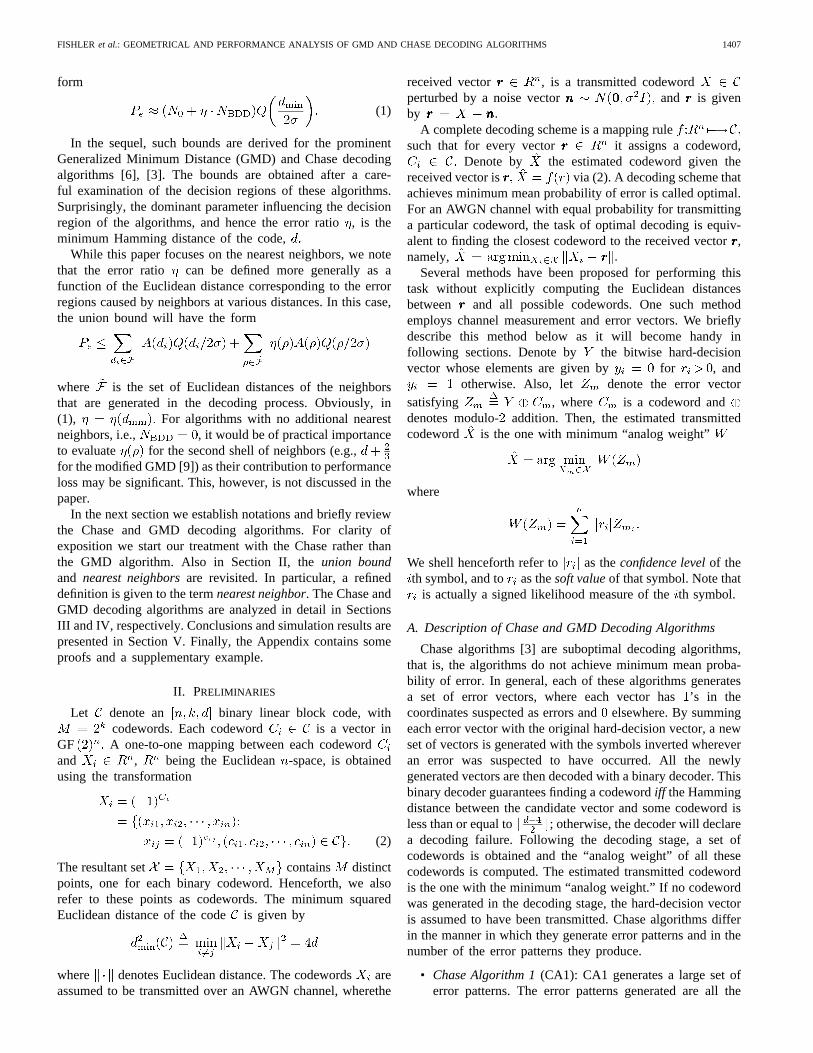
Fig. 2. Chase Algorithm 1,[8; 4; 4] code: volume ratio versus empirical probability ratio.

a small radius , centered on and , respectively.Denote by and by the regions in and ,where decoding error occurs:

. Note that andare the same for all , , and for any “transmitted”codeword. This is evident for , while for it followsfrom the fact that for a binary linear code with the mapping (2),the analyzed algorithms [3], [6], do not make any distinctionbetween codewords or symbol values Since and

are close to the transmitted codeword (relative to thecomplete error region ), the probabilityratio

provides significant information on the relation between acodeword and a noncodeword nearest neighbor in terms oftheir contribution to the error probability. Using as amultiplying factor of yields a better approximation forthe upper bound (5). In general, is defined as the ratiobetween corresponding to the error region whoseclosest point is at distance from and correspondingto the hemisphere-shaped error region at distancefrom

In this work, our attention is restricted to the particularcase since the first term of the union bound,corresponding to the nearest neighbors, usually (and the an-alyzed algorithms [3], [6], are no exception) dominates theerror performance.

Computing involves integrating the term over a vol-ume whose boundaries are rather complex. This is a difficultproblem, for which no explicit expression is known. Oneway of approximating the probability ratio is by usingthe ratio, , between the volumes ofand For small, alternatively for high enough SNR, allthe points contained in the hyper-spheresand haveapproximately the same probability. In light of the above, wecan write

The region is simply a hemisphere, its volume is thus givenby [4] whereThe volume of the region is given by the next theorem.

Theorem 2: For Chase Algorithm 1

Proof: Let be the set of indices such thatNote that is one of the sets

defined from (6). , whose volume is ,can be partitioned into equal and disjoint portions asfollows. Each portion is composed of all the vectors ,such that for every index , has a constant sign.For instance, one such portion is obtained by letting all thesymbols with indices belonging to to have a positivesoft value. It is clear that all portions have the same volume,and the union of all the portions is When is smallenough, the transmitted codeword is the closest codeword to


Fig. 3. Chase Algorithm 2, borders of decision regions for codewordc1: c2 noncodeword;c3 codeword.

every point in Hence, decoding error will occur (within) only if the transmitted codeword is not one of the

generated candidates. It follows from [3, proof of Theorem1] that this occurs only in the portions where all symbolswith indices belonging to have negative soft value.In all other portions, no decoding error will occur as therewill be fewer than hard-decision errors and the transmittedcodeword will be one of the candidates. This leads us to theconclusion that decoding error occurs in only of thevolume . Clearly now, is the same for all

Consequently, for Chase Algorithm 1, we obtain

(11)

and, therefore,

(12)

In fact, the volume ratio is an upper bound on the probabilityratio [5]. The proof is rather lengthy and therefore onlysketched in the following. Partition as into disjointportions. Clearly, there exists one portion , obtained viaisometric mapping of , such that . Allthe portions of are isometrically equivalent (to each other)by construction; however, it can be shown thatis the portionfurthest away from and hence satisfying for

Then clearly

It should be emphasized that the proof is independent of theSNR, and holds for a wide range ofThis is demonstrated inFig. 2 for the code by means of computer simulationThe trace representing the volume ratio is uniformlyhigher than the probability ratio traces corresponding to severalvalues of , ranging from to , and for the entire SNRrange. Similar behavior has also been observed for the rest ofthe algorithms discussed in this work.

B. Chase Algorithm 2

CA2 trades performance for computational complexity. It ismore efficient than CA1, as it considers just a subset of theerror patterns used by the latter. As in Fig. 1, Figs. 3–5 presenttwo-dimensional cross sections of for the extendedHamming code. In Fig. 3, , is a noncodewordnearest neighbor to , and is a nearest neighbor whichis a codeword. Clearly, the noncodeword nearest neighboraffects the probability of decoding error less than a nearestneighbor which is a codeword. In Fig. 4, and , arenoncodeword nearest neighbors to. Here, a nearest neighbor


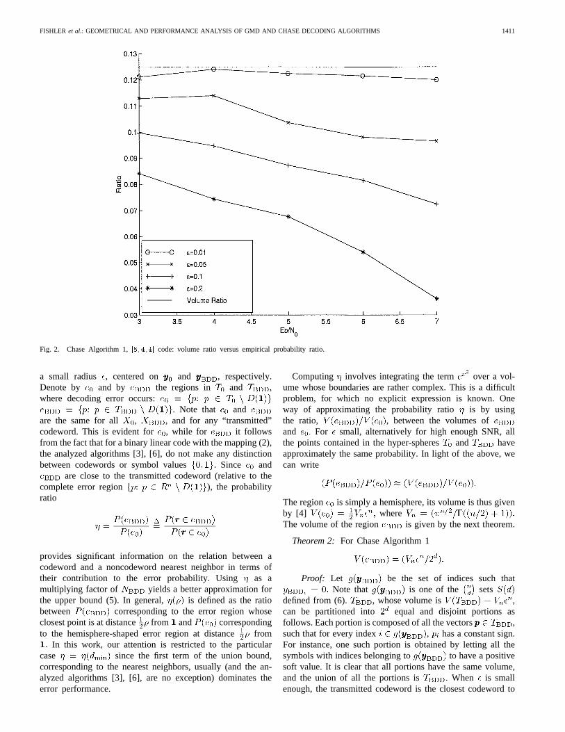
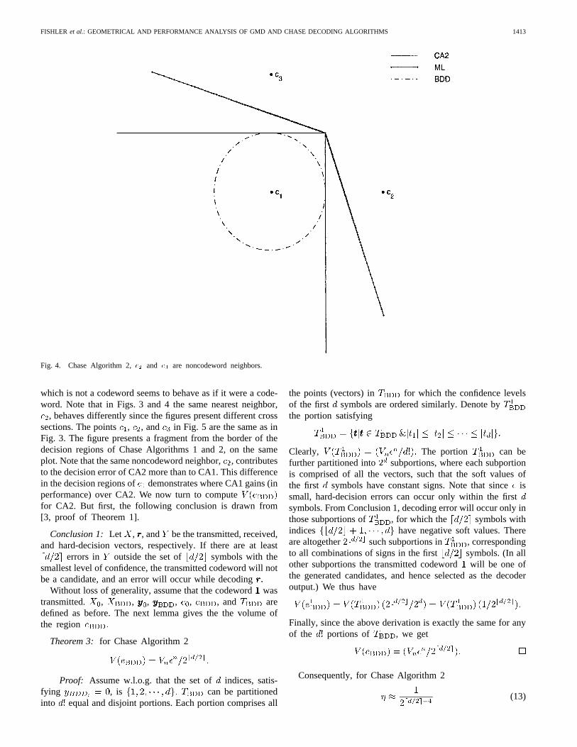
Fig. 4. Chase Algorithm 2,c2 and c3 are noncodeword neighbors.

which is not a codeword seems to behave as if it were a code-word. Note that in Figs. 3 and 4 the same nearest neighbor,

, behaves differently since the figures present different crosssections. The points , , and in Fig. 5 are the same as inFig. 3. The figure presents a fragment from the border of thedecision regions of Chase Algorithms 1 and 2, on the sameplot. Note that the same noncodeword neighbor,, contributesto the decision error of CA2 more than to CA1. This differencein the decision regions of demonstrates where CA1 gains (inperformance) over CA2. We now turn to computefor CA2. But first, the following conclusion is drawn from[3, proof of Theorem 1].

Conclusion 1: Let , , and be the transmitted, received,and hard-decision vectors, respectively. If there are at least

errors in outside the set of symbols with thesmallest level of confidence, the transmitted codeword will notbe a candidate, and an error will occur while decoding

Without loss of generality, assume that the codewordwastransmitted. , , , , , , and aredefined as before. The next lemma gives the the volume ofthe region

Theorem 3: for Chase Algorithm 2

Proof: Assume w.l.o.g. that the set of indices, satis-fying , is can be partitionedinto equal and disjoint portions. Each portion comprises all

the points (vectors) in for which the confidence levelsof the first symbols are ordered similarly. Denote bythe portion satisfying

Clearly, The portion can befurther partitioned into subportions, where each subportionis comprised of all the vectors, such that the soft values ofthe first symbols have constant signs. Note that sinceissmall, hard-decision errors can occur only within the firstsymbols. From Conclusion 1, decoding error will occur only inthose subportions of , for which the symbols withindices have negative soft values. Thereare altogether such subportions in , correspondingto all combinations of signs in the first symbols. (In allother subportions the transmitted codewordwill be one ofthe generated candidates, and hence selected as the decoderoutput.) We thus have

Finally, since the above derivation is exactly the same for anyof the portions of , we get

Consequently, for Chase Algorithm 2

(13)


Fig. 5. Chase Algorithm 1 and 2, different decision borders for the same pointc2:

and, therefore,

(14)

Equations (11) and (13), reveal an interesting property ofChase Algorithms 1 and 2, respectively. The contribution toerror probability of a noncodeword nearest neighbor dropsexponentially with and , for CA1 and CA2, respectivelyAs in the case of CA1, the volume ratio is an upper bound onthe probability ratio. The proof is not much different than forCA1 and is supported by simulation results (not presented inthis paper). Recently, an upper bound has been derived on thebit-error rate (BER) performance of CA2 [8]. This bound isbased on a probabilistic rather than a geometrical method andis more complex to evaluate than the proposed bound.

C. Chase Algorithm 3

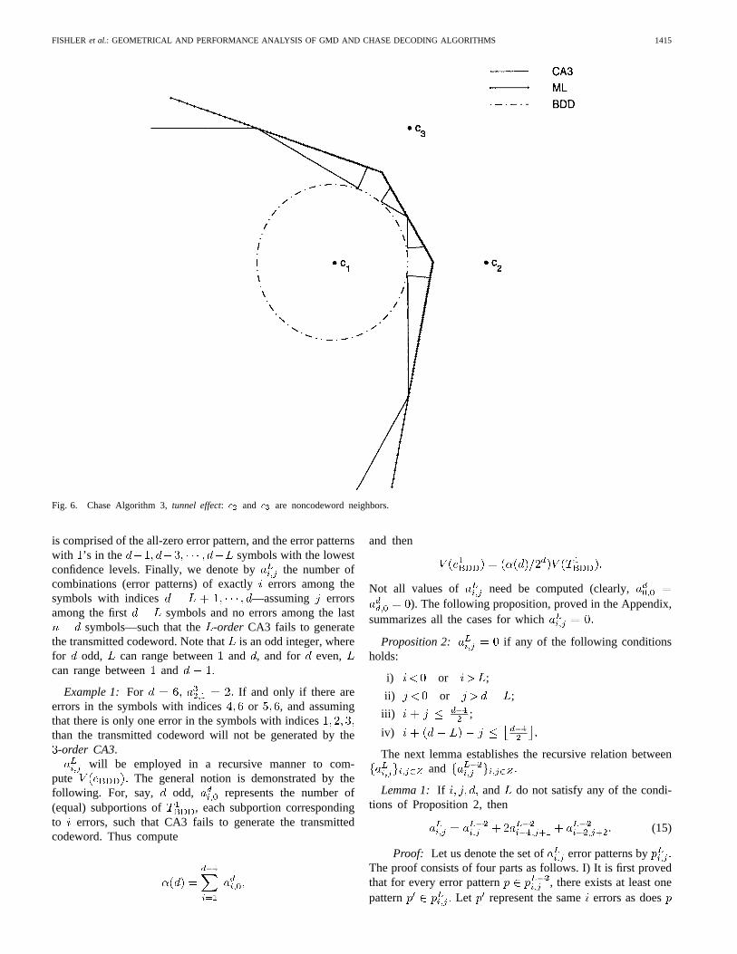
CA3 is the most efficient of the Chase algorithms, the priceis further degradation in performance. The decision regionof CA3 has quite an interesting shape. In Fig. 6 , ,

, and are noncodeword nearest neighbors to In thedepicted cross section, the decision region is not at all tangentto the bounded distance hyper-sphere at the midpointsand as is usually expected. Referring to and , themagnitude of the noise can be greater than , on theimaginary line connecting and , so that there are symbolerrors in the hard-decision vector, yet CA3 decodes correctly.

We refer to this phenomenon as a “tunnel effect.” This figure,however, is misleading. It seems to contradict Proposition 1,for it appears that there exists a hyper-sphere centered on

, in which no decoding error occurs. Fig. 7 presents ashifted and rotated cross section about the midpoint( , , and were chosen such that ), thereis no tunnel here. In fact, the decision region in this crosssection appears just as if were a codeword.

Figs. 6 and 7 also indicate that computing the volume ratiofor CA3 is not an easy task. While for the previous algorithmsa necessary and sufficient condition for decoding error wasderived, for CA3 we develop recursive formulas for computingthe volume ratio and thus eliminating the need for such acondition.

Assume w.l.o.g. that the codewordwas transmitted. Let, , , and be defined as before. Letbe the portion of where decoding error occurs.

Recall that , and that is in thefirst symbols and in the next symbols. canbe further partitioned into equal and disjoint subportions,each of volume Clearly, within , CA3 willfail to decode correctlyiff the transmitted codeword is not oneof the generated candidates. Henceforth, we shall also assumethat the symbols are arranged according to their confidencevalues in a nondecreasing order.

Let us define the -order Chase Algorithm 3as the originalCA3, only considering a smaller set of error patterns. This set


Fig. 6. Chase Algorithm 3,tunnel effect: c2 and c3 are noncodeword neighbors.

is comprised of the all-zero error pattern, and the error patternswith ’s in the symbols with the lowestconfidence levels. Finally, we denote by the number ofcombinations (error patterns) of exactlyerrors among thesymbols with indices —assuming errorsamong the first symbols and no errors among the last

symbols—such that the-order CA3 fails to generatethe transmitted codeword. Note thatis an odd integer, wherefor odd, can range between and , and for even,can range between and

Example 1: For If and only if there areerrors in the symbols with indices or , and assumingthat there is only one error in the symbols with indicesthan the transmitted codeword will not be generated by the-order CA3.

will be employed in a recursive manner to com-pute The general notion is demonstrated by thefollowing. For, say, odd, represents the number of(equal) subportions of , each subportion correspondingto errors, such that CA3 fails to generate the transmittedcodeword. Thus compute

and then

Not all values of need be computed (clearly,). The following proposition, proved in the Appendix,

summarizes all the cases for which

Proposition 2: if any of the following conditionsholds:

i) or ;

ii) or ;

iii) ;

iv)

The next lemma establishes the recursive relation betweenand

Lemma 1: If and do not satisfy any of the condi-tions of Proposition 2, then

(15)

Proof: Let us denote the set of error patterns byThe proof consists of four parts as follows. I) It is first provedthat for every error pattern , there exists at least onepattern Let represent the sameerrors as does


Fig. 7. Chase Algorithm 3, a shifted and rotated version of Fig. 6, no tunnel here.

among the symbols with indices , and no errorsin the indices , . For the error pattern , the

-order CA3 will fail to generate the transmitted codewordin any of the decoding trials:guarantees failure in the trial where the lowest confidencesymbols are complemented; guarantees failure inall the remaining trials. Thus evidently, . II) It isshown that for every error pattern , there existat least two patterns that belong to Simply, let

, respectively, , represent the same errors as does, among the symbols with indices and

one error in the symbol with index , respectively,Using the above arguments, it is straightforward

to verify that III) Finally, for every pattern, there exists at least one pattern The

pattern represents the same errors in the symbols withindices and two errors in the symbols withindices Thus far, we have shown that

IV) The opposite inequality

is easily derived using similar arguments. For every patternas described in Part I above, there exists at least

one pattern , for instance the pattern describedin Part I. For every pair of error patterns asdescribed in Part II above, there exists at least one error pattern

, for instance the pattern described in part IIFor every pattern as described in Part III above,there exists at least one pattern, , for instance the

pattern described in Part III. This concludes the proof of theopposite inequality and the Lemma.

Computing the number of subportions of in whichdecoding error occurs is rather simple using Proposition 2and Lemma 1. For odd, respectively, even, compute ,respectively, , for Let denote the result ofthe summation of all the relevant terms, i.e., forodd

and for even

Then It is now left only toestablish the initial conditions for the recursive relations. When

is even (using Proposition 2), the nonzero initial terms areWhen is odd, the only nonzero

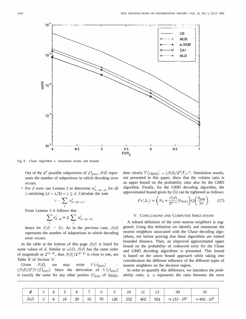
initial term isIn the table at the bottom of the following page, is

listed for some values of It is noteworthy that has thesame order of magnitude as , for the presented values.Thus is close to one, as can be seen in Table II ofSection V. In the Appendix we give the complete derivationof for , as an illustrating example. Also for CA3,simulation results show that the volume ratio is an upper boundon the probability ratio.

In conclusion, since the derivation of is the samefor any other , then clearly


Consequently, for CA3, , and, therefore,

(16)

IV. PERFORMANCE ANALYSIS FOR THE GMD ALGORITHM

The GMD algorithm [6] is one of the first suboptimaldecoding algorithms. It is noteworthy that the results recentlypresented in [12] and [7] suggest a modified GMD algorithmwhich has the same number of nearest neighbors as maximum-likelihood decoding, i.e., In [12] it is provedthat the GMD decoding algorithm is BDD. Moreover, from[12, proof of Theorem 1] it follows that the GMD algorithmdoes not have pseudo nearest neighbors. Thus by a nearestneighbor we shall henceforth be referring to a conventionalnearest neighbor. The above properties allow us to evaluatethe performance of the GMD algorithm by using (5). Thisbound, however, can be tightened by taking into considerationthe different effect of the nearest neighbors on the decisionregion.

Assuming the same geometrical scenario (for ) andnotations as with CA3, we next describe a method for calcu-lating the number of subportions of in which decodingerror occurs. Let us define the-order GMD algorithm asthe original GMD algorithm, only considering a smaller setof erasure patterns. This subset is comprised of the erasurepatterns of the symbols withthe lowest confidence levels. Denote by the number ofcombinations (error patterns) of exactlyhard-decision errors,among the symbols with indices such thatthe -order GMD algorithm fails to generate the transmittedcodeword . The following examples are given to clarify thisdefinition.

Example 2: represents the number of combinationsof errors among the symbols with the lowest confidencelevels, such that the GMD algorithm fails to generate thetransmitted codeword. Note that each combination correspondsto one of the portions of

Example 3: For Since the receivedvector will undergo erasers but it contains no hard-decision errors—the EE decoder will generate the transmittedcodeword.

Example 4: For The received vectorundergoes two erasure trials: the first five, and then firstseven symbols are erased. When the symbols with indices

are in error, the EE decoder will fail to generate thetransmitted codeword in both erasure trials. The same holdsfor the symbols with indices .

will be employed for calculating the number ofsubportions of in which decoding error occurs. Theterms needed for this task can be computed recursively

based on the following two lemmas. Lemma 2 is readilyapplicable for odd values of

Lemma 2: For odd, and

forotherwise.

Proof: Clearly, is irrelevant because the numberof errors cannot be greater than the number of symbols. Also,if , when erasing the symbols with the lowestconfidence levels the transmitted codeword will always begenerated by the EE decoder. The remainder of the proofclosely follows the proof of Lemma 1, with the exception thatGMD decoding uses erasures rather then bit completion.

For even values of the next lemma is employed along withLemma 2 in a complimentary fashion, as will be describedbelow.

Lemma 3: For even, and

Proof: Let us denote the set of error patterns byFirst, it is shown that for every pattern

there exists at least one pattern . is the patternrepresenting errors in the same positions as inFor , theorder- GMD algorithm, which is simply the original GMDalgorithm, will fail to generate the transmitted codeword inany of the decoding trials: the decoding trial with no erasures(conventional algebraic decoder) will fail since ;failure is guaranteed in all remaining decoding trials due to thefact that . Next, it is shown that for every pattern

there exists at least one pattern Letrepresent the same errors as does, and one additional

error in the symbol with the lowest confidence level. Using theabove arguments, it is straightforward to verify thatIn conclusion, we have shown that

The opposite inequality, i.e.,

is derived using similar arguments.The initial conditions, given below, are easy to derive

forotherwise.

The number of subportions of , in which decoding erroroccurs, is obtained in the following manner.

• For odd: use Lemma 2 to determine for allsatisfying . Calculate the sum


Fig. 8. Chase Algorithm 1, simulation results and bounds.

Out of the possible subportions of , repre-sents the number of subportions in which decoding erroroccurs.

• For even: use Lemma 2 to determine for allsatisfying Calculate the sum

From Lemma 3 it follows that

hence let . As in the previous case,represents the number of subportions in which decodingerror occurs.

In the table at the bottom of this page is listed forsome values of Similar to , has the same orderof magnitude as , thus is close to one, seeTable II of Section V.

Given , we may write. Since the derivation of

is exactly the same for any other portion of ,

then clearly . Simulation results,not presented in this paper, show that the volume ratio isan upper bound on the probability ratio also for the GMDalgorithm. Finally, for the GMD decoding algorithm, theapproximated bound given by (5) can be tightened as follows:

(17)

V. CONCLUSIONS AND COMPUTER SIMULATIONS

A refined definition of the termnearest neighborsis sug-gested. Using this definition we identify and enumerate thenearest neighbors associated with the Chase decoding algo-rithms, not before proving that these algorithms are indeedbounded distance. Then, an improved approximated upperbound on the probability of codeword error for the Chaseand GMD decoding algorithms is presented. This boundis based on the union bound approach while taking intoconsideration the different influence of the different types ofnearest neighbors on the decision region.

In order to quantify this difference, we introduce theprob-ability ratio, represents the ratio between the error



TABLE ITHE VOLUME RATIO

contribution of a noncodeword nearest neighbor and a nearestneighbor which is a codeword. Since the probability ratio is toodifficult to calculate directly, we approximateby using theratio between the corresponding error volumes. The improvedbound is of the form

Table I summarizes the obtained volume ratios for theaforementioned decoding algorithms. Specific values ofand should be calculated according to the procedure in thecorresponding sections. In Table II we list the approximated

associated with the decoding algorithm for several valuesof the minimum Hamming distance Note that the volumeratio is exponential in for CA1 and CA2, but not for CA3or GMD. This accounts for the different performance of thealgorithms as obtained from simulations.

Finally, we present some simulation results. A simple ex-ample, the extended Hamming code, has been chosento demonstrate the gain of the improved bound over theunion bound. For each of the bounded distance decodingalgorithms treated in this work, we plot the simulation resultsof: maximum-likelihood decoding (MLD); the bounded dis-

tance algorithm; and a modified union bound (e-MUB) basedon the empirical computation of the ratioAdditionally, we plot the error probability as given by theunion bound (UB); and the modified union bound based onthe volume ratio (MUB).

The results for CA1 are depicted in Fig. 8. As can be seen inthis figure, CA1 is practically optimal. This may be explainedas follows. Although the number of noncodeword nearestneighbors is much higher than , the contribution (toerror probability) of a noncodeword neighbor is considerablysmaller than that of a codeword neighbor. Note that at word-error rate (WER) of the modified bound, MUB,is only 0.25 dB from the actual simulation results, while theunion bound is 0.8 dB away. The modified bound is muchtighter than the union bound also for low SNR. The empiricalbound, e-MUB, is even tighter, only 0.15 dB from the actualresults. The 0.1-dB difference between MUB and e-MUBsuggests that, in the case of CA1, the volume ratio is a veryclose approximation for the probability ratio.

CA2 is much more efficient than CA1. It involves onlyfour algebraic decoding trials as compared to 28 trialsrequired by CA1. Nevertheless, its performance, presentedin Fig. 9, are only 0.125 dB worse than the optimal. Forthis algorithm, at WER of , the empirical modifiedbound, the modified bound, and the original union bound,respectively, are 0.35, 0.45, and 0.7 dB away from thesimulation results. Again, the 0.1-dB difference between



TABLE IISOME SPECIFIC VALUES OF THE VOLUME RATIO

MUB and e-MUB suggests that the volume ratio is a veryclose approximation for the probability ratio.

CA3 is the most efficient among the Chase Algorithms,indeed, for the price of performance. At WER of ,it is 0.2 dB worse than the optimal, as can be seen inFig. 10. The empirical modified bound and the modified boundalmost coincide, 0.35 dB from the ML simulation results.The original union bound is 0.6 dB away from the MLsimulation results. For this algorithm, the volume ratio isevidently closer to the probability ratio, even more than in theprevious algorithms. Unfortunately, this may imply, certainlyfor the presented SNR range, that the probability ratio is

not a tight enough approximation. Note that since all threealgorithms have the same nearest neighbors , the originalunion bound cannot distinguish between them, and is thus thesame for all. As noted in [2], however, in different decodingalgorithms, the same neighbors may differently influence thedecision region. This is evident from the presented simulationresults, and indeed taken into consideration by the modifiedunion bound.

The results for the GMD decoding algorithm are depictedin Fig. 11. The simulation range has been extended here up toSNR 9 dB. At WER of , the GMD algorithm loses0.25 dB as compared to the ML algorithm. That is 0.05 dB


Fig. 11. GMD, simulation results and bounds.

more than CA3, while their decoding complexity and nearestneighbors are identical. The empirical modified bound, themodified bound, and the original union bound, respectively,are 0.3, 0.4, and 0.55 dB, away from the ML simulation results.

APPENDIX

Proof of Proposition 1

Assume (w.l.o.g.) that the codeword was transmit-ted. Let GF be a vector at Hamming distancefromthe all-zero binary codeword There are exactly

such vectors. Denote by the Euclidean version ofvia the transformation (2). has symbols equal to , and

symbols equal to Let be the midpoint betweenand , that is, has symbols equal to , and

symbols equal to . Let be the hyper-sphere with asmall radius centered on

Chase Algorithm 1:Let be the portion of , such thatAccording to [3], decoding

failure will occur for every vector This proves thatis a conventional nearest neighbor, as there is a region withnonzero volume, centered on the midpoint, where decodingerror occurs.

Chase Algorithm 2:The error patterns considered by thisalgorithm are a subset of the patterns considered by CA1.This fact, along with the arguments used for CA1, concludesthe proof.

Chase Algorithm 3:Although it has the same nearestneighbors as do CA1 and CA2, the proof is different inthis case. Assume w.l.o.g. that for For

sufficiently small, such that

can be partitioned into equal and disjoint portions.Each portion corresponds to one combination of ordering ofthe symbols according to their confidence levels. Let

can be further partitioned into equal and disjointsubportions, where each subportion is comprised of all thevectors , such that the soft values of the firstsymbolshave constant sign. Now, consider the subportion ofwherethe first symbols have positive soft values (correctsymbols) and the following symbols have negative softvalues (errors). Evidently, the volume of this subportion isnonzero, and CA3 will fail here. In conclusion, we have shownthat every vector as defined above, satisfies Definition 1, andis thus a conventional nearest neighbor for CA3.

Proof of Proposition 2

Proposition 2 has several conditions, we separately considereach one. Condition i): clearly, there cannot be a negativenumber of hard-decision errors, or more thanerrors, among


symbols. Condition ii): similarly, there cannot be a negativenumber of hard-decision errors, or more than error,among symbols. Condition iii): since the overall numberof errors satisfies , the algebraic decoder willcertainly generate the transmitted codeword in the decodingtrial corresponding to the all-zero error pattern. Conditioniv): represents the number of errors in the first

symbols when those are complimented, i.e., when thepattern is added to the received hard-decisionvector. Since the overall number of errors in this case satisfies

, the algebraic decoder will generatethe transmitted codeword in the decoding trial correspondingto the pattern It is one of the decoding trials of the-orderCA3.

Illustrating Example: Derivation of for Chase Algorithm 3

Clearly, Hence, we compute the fiveterms , where the initial condition in this case is

First, each term is tested for satisfying the conditions ofProposition 2. If does not satisfy any of these conditions(or the initial condition), it is computed recursively usingLemma 1. Thus from Proposition 2 iii) it follows that thefirst two terms of satisfy For each ofthe other two terms Lemma 1 is used recursively as follows:

where

due to Proposition 2 i), and

due to Proposition 2 iv). Therefore,

ACKNOWLEDGMENT

The authors thank M. P. C. Fossorier and S. Lin for preprintof their paper [9]. The authors also thank the referees for theirconstructive comments.

REFERENCES

[1] E. Agrell, “Voronoi regions for binary linear block codes,”IEEE Trans.Inform. Theory, vol. 42, pp. 310–316, 1996.

[2] O. Amrani, and Y. Be‘ery, “Bounded-distance decoding algorithms:decision regions, and pseudo nearest neighbors,”IEEE Trans. Inform.Theory, vol. 44, pp. 3072–3082, 1998.

[3] D. Chase, “A class of algorithms for decoding block codes with channelmeasurement information,”IEEE Trans. Inform. Theory, vol. IT-18, pp.170–182, 1972.

[4] J. H. Conway, and N. J. A. Sloane,Sphere Packings, Lattices andGroups. New York: Springer-Verlag, 1993.

[5] E. Fishler, “Nearest neighbors, decision regions and performance anal-ysis of Chase and GMD decoding algorithms,” M.Sc. thesis, Tel-AvivUniv., Tel-Aviv, Israel, Sept. 1997.

[6] G. D. Forney, Jr. “Generalized minimum distance decoding,”IEEETrans. Inform. Theory, vol. IT-12, pp. 125–131, 1966.

[7] G. D. Forney, Jr. and A. Vardy, “Generalized minimum distancedecoding of Euclidean-space codes and lattices,”IEEE Trans. Inform.Theory, vol. 42, pp. 1992–2026, 1996.

[8] M. P. C. Fossorier and S. Lin, “Soft-decision decoding of linear blockcodes based on ordered statistics,”IEEE Trans. Inform. Theory, vol. 41,pp. 1379–1396, 1995.

[9] , “A unified method for evaluating the error-correcting radius ofreliability-based soft decision algorithms for linear block codes,”IEEETrans. Inform. Theory, vol 44, pp. 691–700, 1998.

[10] T. Kaneko, T. Nishijima, H. Inazumi, and S. Hirasawa, ”An efficientmaximum-likelihood-decoding algorithm for linear block codes withalgebraic decoder,”IEEE Trans. Inform. Theory, vol. 40, pp. 320–327,1994.

[11] H. Tanaka and K. Kakigahara, “Simplified correlation decoding byselecting possible codewords using erasure information,”IEEE Trans.Inform. Theory, vol. IT-29, pp. 743–748, 1983.

[12] B.-Z. Shen, K. K. Tzeng, and C. Wang, “A bounded-distance decodingalgorithm for binary linear block codes achieving the minimum effectiveerror coefficient,”IEEE Trans. Inform. Theory, vol. 42, pp. 1987–1991,1996.

geometrical and performance analysis of gmd and chase decoding algorithms

Documents