geometric inequalities and generalized ricci bounds...

GEOMETRIC INEQUALITIES AND GENERALIZED RICCIBOUNDS IN THE HEISENBERG GROUP∗

NICOLAS JUILLET

Abstract. We prove that no curvature-dimension bound CD(K, N) holds inany Heisenberg group Hn. On the contrary the measure contraction propertyMCP (0, 2n + 3) holds and is optimal for the dimension 2n + 3. For thenon-existence of a curvature-dimension bound, we prove that the generalized“geodesic” Brunn-Minkowski inequality is false in Hn. We also show in anew and direct way, (and for all n ∈ N\{0}) that the general “multiplicative”Brunn-Minkowski inequality with dimension N > 2n + 1 is false.

Introduction

The Heisenberg group Hn turns up both in many parts of mathematics (see[25]) and in other scientific or technical domains. A reason for this is that it isthe most basic and representative space of sub-Riemannian geometry, playing therole of RN in Riemannian geometry. Many analytical tools have been developed inboth settings. In particular Hn and RN both have a doubling measure and satisfya Poincare inequality. This last setting has proved to be very efficient as a minimalframework permitting to generalize conformal geometry to some metric measurespaces (see [13] and the references therein). Recent developments tend to improvethis analysis and introduce for some spaces analysis of second order. In particularit was very challenging to define metric spaces with a lower bound on the curvature.For sectional curvature, Alexandrov spaces were defined more than fifty years ago(see [6]). For Ricci curvature an amazing theory has been recently developed inde-pendently (but using essentially the same ideas) by Sturm (see [27], [28]) and byLott and Villani (see [17], [18]) in terms of geometric curvature-dimension conditionCD(K, N) (The definition is different from the curvature-dimension of Bakry andEmery defined in [3]).

For many metric measure spaces, this very recent condition is stronger thanthe condition that there exists a Poincare inequality and the measure is doubling.It uses an old probability tool: optimal transport of measure. This theory dealswith the so-called Monge-Kantorovich problem, namely the problem of transport-ing one probability measure into another one whilst minimizing a transport cost(usually the square of the distance). For Riemannian manifolds and two absolutelycontinuous measures, McCann proved that there is a unique geodesic interpola-tion between them (see [19]) and studied the particular expression it takes. Fromthis Cordero-Erausquin, McCann and Schmuckenschlager explained in [8] that theoptimal transport of measure has a particular form if the Ricci curvature of the

2000 Mathematics Subject Classification. 28A75.∗Preliminary version in preprint of SFB 611 (Bonn) under the name “Ricci curvature bounds

and geometric inequalities in the Heisenberg group”.

1

2 NICOLAS JUILLET

manifold is bounded below. In particular the transported measure has a relativeentropy whose level of convexity along the transport depends on the lower boundof the Ricci curvature. Inspired by this observation Lott, Sturm and Villani definedthe curvature-dimension condition CD(K, N) and developed a theory of syntheticRicci curvature in metric measure spaces. An other essential fact is that inspiredby [19], Ambrosio an Rigot recently proved in [1] that the geodesic solutions ofthe Monge problem in the Heisenberg group Hn have a similar expression as theone for the Riemannian manifolds. We answer this question in this paper whethercurvature-dimension condition also holds in this space.

The measure contraction property MCP (K, N) is another geometrical propertythat involves curves in the space of measures on a given metric measure space. In acertain sense, the definition of the MCP involves curves in the space of measures oneof whose extremities corresponds to a Dirac mass. The other measure is contractedonto this Dirac mass and this contraction reveals some geometrical aspects of thespace. As CD, the measure contraction property can be seen as a generalizationof the Ricci lower bound of a Riemannian manifold. As written in the appendix,under the hypothesis that there is almost surely a unique geodesic between twopoints (this is the case in Hn) the curvature-dimension condition CD(K, N) impliesthe measure contraction MCP (K, N) and this last property implies that the metricmeasure space satisfies a Poincare inequality and is doubling.

In this paper we prove the following theorem:

Main Theorem. Let n be a non negative integer. We consider (Hn, dCC ,L2n+1),the n-th Heisenberg group with its Carnot-Caratheodory distance and the Lebesguemeasure of R2n+1. Then:

• For every N ∈ [1,+∞] and every K ∈ R, the geometric curvature-dimensionbound CD(K, N) does not hold in (Hn, dCC ,L2n+1).

• For (N,K) ∈ [1,+∞[×R, the measure contraction property MCP (K, N)holds in (Hn, dCC ,L2n+1) if and only if N ≥ 2n + 3 and K ≤ 0.

A first surprise is that the geometric curvature-dimension and the measure con-traction property behave differently. It is known that these properties are differentbut they are quite close: For a N -dimensional Riemannian manifold (M, g), theconditions CD(K, N) and MCP (K, N) are both equivalent to the property of hav-ing a Ricci curvature greater than Kg (Compare also with the Bakry and Emerycurvature-dimension condition for the Laplace-Betrami operator in [2]). The sec-ond surprise is the dimension 2n + 3 that appears in the second item. As far as Iknow it has no classic significance and this may be the first time it arises in relationto the Heisenberg group.

In the first section, we give a short presentation of the Heisenberg group Hn

(n ∈ N\{0}) and its geodesics. We also introduce two maps that will be helpful inthe following sections: the geodesic-inversion map I and the intermediate pointsmap M. At the beginning of the second section we give the definition of CD(K, N)and MCP (K, N) for K = 0 which is the only interesting case. We prove the secondpart of the Main Theorem in Theorem 2.3. The last section is devoted to a proofof the fact that there is no geodesic Brunn-Minkowski inequality in the Heisenberggroup: it is the keystone of Theorem 3.3 which corresponds to the first part of theMain Theorem. Remark 3.4 of this section deals with MCP and CD for non-zerocurvature parameters. This completes the Main Theorem. We also mention the

GENERALIZED RICCI BOUNDS IN THE HEISENBERG GROUP 3

multiplicative Brunn-Minkowski inequality and sketch the fact that this inequalitydoes not hold in any dimension strictly greater than the topological dimension(i.e. 2n + 1). In the appendix, we sketch relations between the geodesic Brunn-Minkowski inequality, CD(K, N), MCP (K, N) and the Poincare inequality plusdoubling measure.

1. The Heisenberg Group and its Geodesics

1.1. The Heisenberg group. Let n be a non-negative integer. In this section wegive a short presentation of the Heisenberg group Hn as a metric measure spaceequipped with the Lebesgue measure L2n+1 and Carnot-Caratheodory metric dCC .As a set Hn can be written in the form R2n+1 ' Cn ×R and an element of H1 canalso be written as (z, t) = (z1, · · · , zn, t) where zk := xk + iyk ∈ C for 1 ≤ k ≤ nand t ∈ R. The group structure of Hn is given by:

(z1, · · · , zn, t) · (z′1, · · · , z′n, t′) =

(z1 + z′1, · · · , zn + z′n, t + t′ + 2

n∑k=1

=(zkz′k)

)where = denotes the imaginary part of a complex number. Hn is then a Lie groupwith neutral element 0Hn := (0, 0) and inverse element (−z,−t). The set L ={(z, t) ∈ Hn | z = 0} is the center of the group and will play an important role.Throughout this paper, τp : Hn → Hn will be the left translation

τp(q) = p · q

where p, q ∈ Hn. This map is affine and its vectorial part has the determinant 1.It follows that the Haar measure of Hn is the Lebesgue measure L2n+1 of R2n+1

which is left (and actually also right) invariant. For λ > 0, we denote by δλ thedilation

δλ(z, t) = (λz, λ2t).

The measures behaviour under dilation is also good:

L2n+1(δλ(E)) = λ2n+2L2n+1(E)(1)

if λ ≥ 0 and E is a measurable set.In order to define the Carnot-Caratheodory metric, we consider the Lie algebra

associated to Hn. This is the vector space of left-invariant vector fields. A basis forthis vector space is given by

(−→X 1, · · · ,

−→Xn,

−→Y 1, · · · ,

−→Y n,

−→T)

where

−→Xk = ∂xk

+ 2yk∂t

−→Y k = ∂yk

− 2xk∂t

−→T = ∂t.

Roughly speaking, the Carnot-Caratheodory distance between two points p and qis the infimum of the lengths of the horizontal curves connecting p and q. By ahorizontal curve we mean an absolutely continuous curve γ : [0, r] → Hn whosederivative γ′(s) is spanned by {

−→X 1(s), · · · ,

−→Xn(s),

−→Y 1(s), · · · ,

−→Y n(s)} in almost all

points s. The length of this curve is then

length(γ) =∫ r

0

‖γ′(s)‖ ds

4 NICOLAS JUILLET

where ‖∑n

k=1(ak−→Xk + bk

−→Y k)‖2 =

∑nk=1(a

2k + b2

k). The value of the Carnot-Caratheodory distance between p and q is then

dCC(p, q) := inf length(γ)(2)

where the infimum is taken over all horizontal curves γ connecting p and q. TheChow Theorem (see for example [20]) ensures that this set is not empty. TheCarnot-Caratheodory metric (like the Lebesgue measure) behaves well under trans-lation τp and dilation δλ. It is left-invariant:

dCC(τpq, τpq′) = dCC(q, q′)(3)

and

dCC(δλ(q), δλ(q′)) = λdCC(q, q′)(4)

for λ > 0. Because of (3), the Hausdorff measure (derived from dCC) is a Haarmeasure. With the correct dimension, this measure is then proportional to theLebesgue measure. By (1) and (4), it follows that the Hausdorff dimension of(Hn, dCC) is 2n + 2.

The metric space (Hn, dCC) is complete and separable. Another essential factis that the topology given by dCC is the usual topology on R2n+1. The Hausdorffdimension is then different from the topological dimension (2n+2 6= 2n+1), whichis considered by some authors as the definition for a fractal set.

1.2. A geodesic space. Let us first give the terminology that we will use in thispaper.

Definition 1.1. Let (X, d) be a metric space. Let m0 and m1 be two points of thisset. An s-intermediate point between m0 and m1 is a point ms such that

d(m0,ms) = sd(m0,m1) and

d(ms,m1) = (1− s)d(m0,m1).

A geodesic from m0 to m1 is a continuous map γ defined on a segment [a, b] (witha < b) such that for every a′, b′, c ∈ [a, b] with a′ ≤ c ≤ b′, the point γ(c) is ac−a′

b′−a′ -intermediate point between γ(a′) and γ(b′). A normal geodesic is a geodesicdefined on [0, 1]. A local geodesic is a curve γ defined on an interval I, such thatfor any point s in the interior of I there is an ε > 0 such that [s− ε, s + ε] ⊂ I andγ |[s−ε,s+ε] is a geodesic. The metric space (X, d) is said to be a geodesic space ifthere is a geodesic between any two points of X.

We now come to the geodesics of Hn. The infimum in (2) turns out to actuallybe a minimum. We have the following proposition, which can be found in [1] forexample:

Proposition 1.2. The metric space (Hn, dCC) is a geodesic space. Moreover everygeodesic between two points p and q of Hn is horizontal and has length dCC(p, q).

The equations of the local geodesics of Hn have been known since Gaveau’s paper[11]. In [1] Ambrosio and Rigot give explicitly the cut locus of local geodesics passingthrough 0H. See also [20] for the similarities with the Dido problem. In this paper,we will investigate how the measure is transported along the geodesics: to do thiswe need to know their equations. Because the Carnot-Caratheodory distance andhence the geodesics are left-invariant, it is enough to know the equations of the


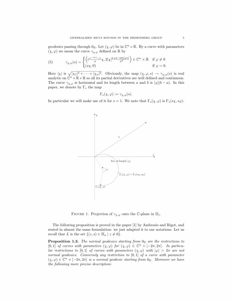
geodesics passing through 0H. Let (χ, ϕ) be in Cn×R. By a curve with parameters(χ, ϕ) we mean the curve γχ,ϕ defined on R by

γχ,ϕ(s) =

{(i e−iϕs−1

ϕ χ, 2|χ|2 ϕs−sin(ϕs)ϕ2

)∈ Cn × R if ϕ 6= 0

(sχ, 0) if ϕ = 0.(5)

Here |χ| is√|χ1|2 + · · ·+ |χn|2. Obviously, the map (χ, ϕ, s) → γχ,ϕ(s) is real

analytic on Cn×R×R so all its partial derivatives are well defined and continuous.The curve γχ,ϕ is horizontal and its length between a and b is |χ|(b − a). In thispaper, we denote by Γs the map

Γs(χ, ϕ) := γχ,ϕ(s).

In particular we will make use of it for s = 1. We note that Γs(χ, ϕ) is Γ1(sχ, sϕ).

x

y

χ

ϕ

Arc of length |χ|

Γ1(χ, ϕ)

Γs(χ, ϕ) = Γ1(sχ, sϕ)

Figure 1. Projection of γχ,ϕ onto the C-plane in H1.

The following proposition is proved in the paper [1] by Ambrosio and Rigot, andstated in almost the same formulation: we just adapted it to our notations. Let usrecall that L is the set {(z, s) ∈ Hn | z 6= 0}.

Proposition 1.3. The normal geodesics starting from 0H are the restrictions to[0, 1] of curves with parameters (χ, ϕ) for (χ, ϕ) ∈ Cn × [−2π, 2π]. In particu-lar restrictions to [0, 1] of curves with parameters (χ, ϕ) with |ϕ| > 2π are notnormal geodesics. Conversely any restriction to [0, 1] of a curve with parameter(χ, ϕ) ∈ Cn × [−2π, 2π] is a normal geodesic starting from 0H. Moreover we havethe following more precise description:

6 NICOLAS JUILLET

• For any p = (0, t) ∈ L∗, normal geodesics from 0H to p are exactly therestrictions to [0, 1] of the curves with parameters (χ, t

|t|2π) where χ is an

element of the sphere of vectors with norm√

π|t|.• For any p ∈ Hn\L there exists a unique normal geodesic connecting 0H

and p. This is the restriction to [0, 1] of a curve of parameters (χ, ϕ) with|ϕ| < 2π.

Remark 1.4. The curves with parameters (a+ ib, v, r) from [1] (with |a|2 + |b|2 = 1)have constant speed equal to one and are in fact curves with parameters (a + ib, v)restricted to [0, r]. The restrictions to [0, 1] of the curves with parameters (χ, ϕ)have length |χ| and are simply the curves s ∈ [0, 1] → expH(sχ, sϕ/4) where expHis the Heisenberg-exponential map from the end of [1].

Remark 1.5. The map s → δs(p) is not a geodesic.

We give a corollary of Proposition 1.3 for local geodesics.

Corollary 1.6. The curve with parameters (χ, ϕ) is a local geodesic. More preciselythe restriction of γχ,ϕ to [a, b] is a geodesic if and only if (b−a)|ϕ| ≤ 2π. Moreoverthis is the unique geodesic defined on [a, b] if and only if (b− a)|ϕ| < 2π.

Proof. The case a = 0 and γχ,ϕ(a) = 0H is contained in Proposition 1.3. Tocomplete the proof we compute the left translation of the curve mapping γ,ϕ(a) to0H and obtain

γχ,ϕ(a)−1 · γχ,ϕ(a + s) = γχ′,ϕ(s)with χ′ = e−iϕaχ. The proposition follows from this equation and the fact thatdCC is left-invariant. �

We set D1 := (Cn\0)×] − 2π, 2π[ and similarly Ds := (Cn\0)×] − 2sπ, 2sπ[for s ∈ [0, 1]. The following proposition is a second and important corollary ofProposition 1.3:

Proposition 1.7. The map Γ1 is a C∞-diffeomorphism from D1 to Hn\L. Simi-larly for s ∈ [−1, 0[∪]0, 1[, the map Γs is a C∞-diffeomorphism from D1 to Γ1(D|s|).

Proof. For general s the assertion is a direct consequence of the case s = 1 and therelation Γs(χ, ϕ) = Γ1(sχ, sϕ). With Proposition 1.3, it is clear that Γ1 is one-to-one on D1 and it is C∞-differentiable because it is real analytic. We postpone theproof that its Jacobian determinant does not vanish to Proposition 1.12 at the endof this section. �

We introduce two helpful maps: the intermediate-points map M and geodesic-inversion map I. The left-invariance of the Carnot-Caratheodory metric tells uswhether or not there is a unique normal geodesic between two given points. Ifp = (z, t) and q = (z′, t′), the isometry τp−1 maps p to 0H and q to p−1·q = (z−z′, t′′)for some t′′ in R. It follows from Proposition 1.3 that there is a unique normalgeodesic from p to q if and only if z 6= z′ or p = q. We will denote the open set{(p, q) ∈ (Hn)2 | zp 6= zq} = {(p, q) ∈ (Hn)2 | p−1 · q /∈ L} by U . On this set wedefine our first map.

Definition 1.8. We define the intermediate-points map M from the set U × [0, 1] toHn by

M(p, q, s) = τp ◦ Γs ◦ Γ−11 ◦ τp−1(q).


The point M(p, q, s) is actually the unique s-intermediate point between p andq. It is a s-intermediate point when p = 0H because Γs ◦ Γ−1

1 (γχ,ϕ(1)) is γχ,ϕ(s)for (χ, ϕ) ∈ D1. The general case follows from the left-invariance of the Carnot-Caratheodory metric. Moreover M(p, q, s) is the unique s-intermediate point be-tween p and q because there is a unique normal geodesic from p to q (the pair(p, q) is in U) and because the s-intermediate points in a geodesic space lie on thegeodesics connecting two points.

In the following sections, we will extend M in (two) different ways to (Hn)2 ×[0, 1]. Using the proposition 1.7 and recalling that τp is affine, we have the followingregularity lemma.

Lemma 1.9. The map M is measurable. It is C∞ on U×]0, 1[. The curve s ∈[0, 1] →M(p, q, s) is the unique normal geodesic from p to q.

Let us now introduce the geodesic-inversion map I.

Definition 1.10. We define the geodesic-inversion map I on Hn\L by I(p) = Γ−1 ◦Γ−1

1 (p).

The name comes from the fact that for (χ, ϕ) ∈ D1 and s ∈ [−1, 1] we have byProposition 1.7:

I(γχ,ϕ(s)) = I(Γ(sχ, sϕ))

= Γ−1 ◦ Γ−11 (Γ1(sχ, sϕ))

= Γ−1(sχ, sϕ)

= γχ,ϕ(−s).

It follows that I ◦I is the identity on Hn\L. That is why for any p ∈ Hn we will call(p, I(p)) a pair of I-conjugate points. We now establish the connection between Mand I.

Lemma 1.11. Let p be in Hn\L. Then M(I(p), p, 1/2) is well defined and is 0Hif and only if the ϕ-coordinate of Γ−1

1 (p) verifies |ϕ| < π , i.e when p ∈ Γ1(D1/2).

Proof. Proposition 1.3 says that p = Γ1(χ, ϕ) for some |ϕ| < 2π. Moreover thedefinition of I implies that I(p) = Γ−1(χ, ϕ). Therefore we have to say whenM(γχ,ϕ(−1), γχ,ϕ(1), 1/2) exists and if it is 0H.

It follows from equation (5) that the z-coordinates of γχ,ϕ(−1) and γχ,ϕ(1) areequal if and only if |ϕ| = π. Therefore (γχ,ϕ(−1), γχ,ϕ(1)) ∈ U if and only if |ϕ| 6= π.In this case there is a unique geodesic δ on [−1, 1] between the two points and wecan define the midpoint

δ(0) = M(δ(−1), δ(1), 1/2) = M(γχ,ϕ(−1), γχ,ϕ(1), 1/2).

If |ϕ| < π then 2|ϕ| < 2π. In this case the curve δ is the restriction of γχ,ϕ

to [−1, 1] because by Corollary 1.6 both maps are the unique geodesic defined on[−1, 1] that goes from I(p) to p. The midpoint is then δ(0) = γχ,ϕ(0) = 0H.

If π < |ϕ| < 2π we argue by contradiction. Assume that δ(0) = 0H. Thenby Proposition 1.3, the curve δ |[0,1] is the unique normal geodesic from 0H top = γχ,ϕ(1) and s ∈ [0, 1] → δ(−s) is the unique normal geodesic between 0H andI(p) = γχ,ϕ(−1). It follows that δ is γχ,ϕ on [0, 1] and [−1, 0] contradicting the factthat |ϕ| > π. (For 2|ϕ| > 2π, Corollary 1.6 shows that the restriction to [−1, 1]of γχ,ϕ is not a geodesic and consequently can not be δ.) Hence M(p, I(p), 1/2) isnot 0H. �

8 NICOLAS JUILLET

As mentioned above, we present the computation of the Jacobian determinant.To prove Proposition 1.7, we only need to prove that the Jacobian of Γ1 doesnot vanish. This fact is mentioned in [1] where the authors state that Γ1 is adiffeomorphism (in fact in this paper χ is given by its polar coordinates (|χ|, χ

|χ| )).The result of the calculation is given for H1 in the paper of Monti (see [21]). Wenow give all the details of this computation for every n ∈ N\{0} because we donot only need the fact that the Jacobian determinant does not vanish, but also itsexact value.

Proposition 1.12. The Jacobian determinant of Γ1 is given by

Jac(Γ1)(χ, ϕ) =

22n+2|χ|2(

sin(ϕ/2)ϕ

)2n−1sin(ϕ/2)−(ϕ/2) cos(ϕ/2)

ϕ3 for ϕ 6= 0,

|χ|2/3 otherwise.

It does not vanish on D1.

Proof. We start by writing exactly what Γ1 is:

Γ1(χ, ϕ) =

{(i e−iϕ−1

ϕ χ1, · · · , i e−iϕ−1ϕ χn, 2|χ|2 ϕ−sin(ϕ)

ϕ2

)if ϕ 6= 0,

(χ, 0) otherwise

where |χ|2 = |χ1|2 + · · · + |χn|2. We start by calculating Jac(Γ1) = det(DΓ1) forϕ 6= 0. The case ϕ = 0 is obtained as a limit.

We first have to compute the real derivative of Γ1, i.e. the derivative of Γ1 as amap from R2n+1 to R2n+1. We write DΓ1 as a matrix

(P CR q

)where the block P is

made of the 2n first rows and columns. If we identify complex numbers with 2× 2matrices (a + ib is

(a −bb a

)), we can write P as an n× n complex matrix i e−iϕ−1

ϕ In

where In is the identity matrix of Mn(C). The column C is ( e−iϕ

ϕ −i e−iϕ−1ϕ2 )χ seen as

a R2n vector, the row R is (4x1ϕ−sin(ϕ)

ϕ2 , 4y1ϕ−sin(ϕ)

ϕ2 , · · · , 4xnϕ−sin(ϕ)

ϕ2 , 4ynϕ−sin(ϕ)

ϕ2 ),

and the real number q is 2|χ|2(

2sin(ϕ)ϕ3 − 1+cos(ϕ)

ϕ2

).

It is difficult to compute directly the determinant of(

P CR q

)in any point. Because

of this we now prove that if |χ| = |χ′|, then Jac(Γ1)(χ, ϕ) = Jac(Γ1)(χ′, ϕ). LetT be a unitary C-linear map so that T (χ) = χ′. Consider now T ′ defined byT ′(χ, ϕ) = (T (χ), ϕ). Then it is not difficult to see that Γ1 ◦T ′ = T ′ ◦Γ1. It followsthat (Jac(Γ1)◦T ′)·detR(T ′) = detR(T ′)·Jac(Γ1) and hence we have Jac(Γ1)(χ, ϕ) =Jac(Γ1)(χ′, ϕ). We use this relation to simplify the computation by choosing χ′ =(0, · · · , 0, |χ|). With this new vector χ′, most of the entries of C and R are equalto zero, so we can calculate the determinant of DΓ1 =

(P CR q

)by blocks. We get

that Jac(Γ1)(χ, ϕ) is the product of∣∣∣∣ sin(ϕ)/ϕ (1− cos(ϕ))/ϕ(cos(ϕ)− 1)/ϕ sin(ϕ)/ϕ

∣∣∣∣n−1

with ∣∣∣∣∣∣∣∣sin(ϕ)/ϕ (1− cos(ϕ))/ϕ |χ|( cos(ϕ)

ϕ − sin(ϕ)ϕ2 )

(cos(ϕ)− 1)/ϕ sin(ϕ)/ϕ |χ|(− sin(ϕ)ϕ − cos(ϕ)−1

ϕ2 )

4|χ|ϕ−sin(ϕ)ϕ2 0 2|χ|2

(2 sin(ϕ)

ϕ3 − 1+cos(ϕ)ϕ2

)∣∣∣∣∣∣∣∣ .


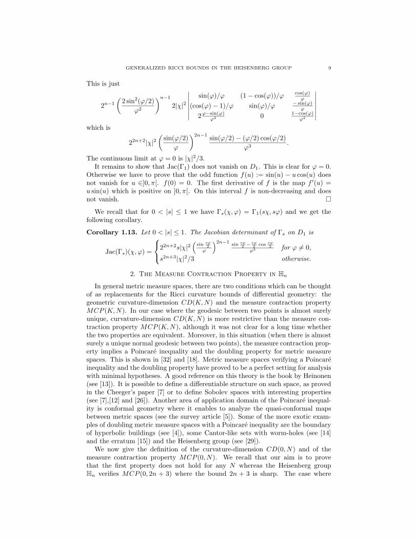
This is just

2n−1

(2 sin2(ϕ/2)

ϕ2

)n−1

2|χ|2

∣∣∣∣∣∣∣sin(ϕ)/ϕ (1− cos(ϕ))/ϕ cos(ϕ)

ϕ

(cos(ϕ)− 1)/ϕ sin(ϕ)/ϕ − sin(ϕ)ϕ

2ϕ−sin(ϕ)ϕ2 0 1−cos(ϕ)

ϕ2

∣∣∣∣∣∣∣which is

22n+2|χ|2(

sin(ϕ/2)ϕ

)2n−1 sin(ϕ/2)− (ϕ/2) cos(ϕ/2)ϕ3

.

The continuous limit at ϕ = 0 is |χ|2/3.It remains to show that Jac(Γ1) does not vanish on D1. This is clear for ϕ = 0.

Otherwise we have to prove that the odd function f(u) := sin(u) − u cos(u) doesnot vanish for u ∈]0, π[. f(0) = 0. The first derivative of f is the map f ′(u) =u sin(u) which is positive on ]0, π[. On this interval f is non-decreasing and doesnot vanish. �

We recall that for 0 < |s| ≤ 1 we have Γs(χ, ϕ) = Γ1(sχ, sϕ) and we get thefollowing corollary.

Corollary 1.13. Let 0 < |s| ≤ 1. The Jacobian determinant of Γs on D1 is

Jac(Γs)(χ, ϕ) =

22n+2s|χ|2(

sin sϕ2

ϕ

)2n−1sin sϕ

2 − sϕ2 cos sϕ

2ϕ3 for ϕ 6= 0,

s2n+3|χ|2/3 otherwise.

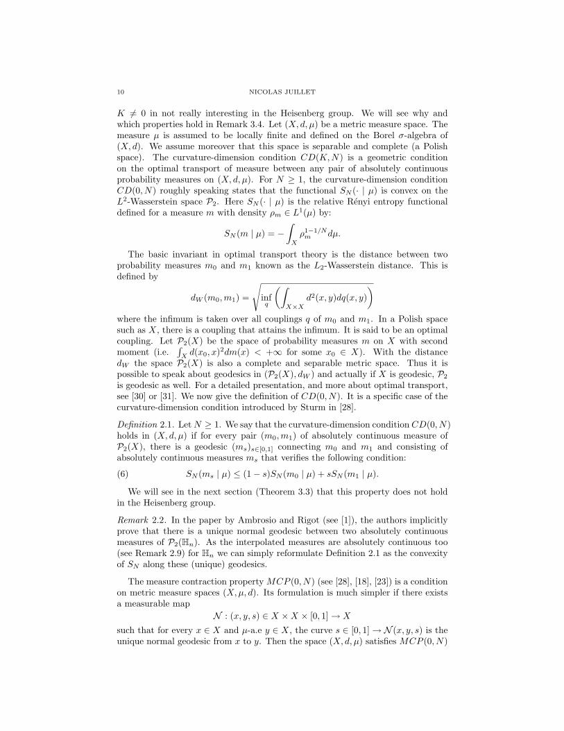
2. The Measure Contraction Property in Hn

In general metric measure spaces, there are two conditions which can be thoughtof as replacements for the Ricci curvature bounds of differential geometry: thegeometric curvature-dimension CD(K, N) and the measure contraction propertyMCP (K, N). In our case where the geodesic between two points is almost surelyunique, curvature-dimension CD(K, N) is more restrictive than the measure con-traction property MCP (K, N), although it was not clear for a long time whetherthe two properties are equivalent. Moreover, in this situation (when there is almostsurely a unique normal geodesic between two points), the measure contraction prop-erty implies a Poincare inequality and the doubling property for metric measurespaces. This is shown in [32] and [18]. Metric measure spaces verifying a Poincareinequality and the doubling property have proved to be a perfect setting for analysiswith minimal hypotheses. A good reference on this theory is the book by Heinonen(see [13]). It is possible to define a differentiable structure on such space, as provedin the Cheeger’s paper [7] or to define Sobolev spaces with interesting properties(see [7],[12] and [26]). Another area of application domain of the Poincare inequal-ity is conformal geometry where it enables to analyze the quasi-conformal mapsbetween metric spaces (see the survey article [5]). Some of the more exotic exam-ples of doubling metric measure spaces with a Poincare inequality are the boundaryof hyperbolic buildings (see [4]), some Cantor-like sets with worm-holes (see [14]and the erratum [15]) and the Heisenberg group (see [29]).

We now give the definition of the curvature-dimension CD(0, N) and of themeasure contraction property MCP (0, N). We recall that our aim is to provethat the first property does not hold for any N whereas the Heisenberg groupHn verifies MCP (0, 2n + 3) where the bound 2n + 3 is sharp. The case where

10 NICOLAS JUILLET

K 6= 0 in not really interesting in the Heisenberg group. We will see why andwhich properties hold in Remark 3.4. Let (X, d, µ) be a metric measure space. Themeasure µ is assumed to be locally finite and defined on the Borel σ-algebra of(X, d). We assume moreover that this space is separable and complete (a Polishspace). The curvature-dimension condition CD(K, N) is a geometric conditionon the optimal transport of measure between any pair of absolutely continuousprobability measures on (X, d, µ). For N ≥ 1, the curvature-dimension conditionCD(0, N) roughly speaking states that the functional SN (· | µ) is convex on theL2-Wasserstein space P2. Here SN (· | µ) is the relative Renyi entropy functionaldefined for a measure m with density ρm ∈ L1(µ) by:

SN (m | µ) = −∫

X

ρ1−1/Nm dµ.

The basic invariant in optimal transport theory is the distance between twoprobability measures m0 and m1 known as the L2-Wasserstein distance. This isdefined by

dW (m0,m1) =

√infq

(∫X×X

d2(x, y)dq(x, y))

where the infimum is taken over all couplings q of m0 and m1. In a Polish spacesuch as X, there is a coupling that attains the infimum. It is said to be an optimalcoupling. Let P2(X) be the space of probability measures m on X with secondmoment (i.e.

∫X

d(x0, x)2dm(x) < +∞ for some x0 ∈ X). With the distancedW the space P2(X) is also a complete and separable metric space. Thus it ispossible to speak about geodesics in (P2(X), dW ) and actually if X is geodesic, P2

is geodesic as well. For a detailed presentation, and more about optimal transport,see [30] or [31]. We now give the definition of CD(0, N). It is a specific case of thecurvature-dimension condition introduced by Sturm in [28].

Definition 2.1. Let N ≥ 1. We say that the curvature-dimension condition CD(0, N)holds in (X, d, µ) if for every pair (m0,m1) of absolutely continuous measure ofP2(X), there is a geodesic (ms)s∈[0,1] connecting m0 and m1 and consisting ofabsolutely continuous measures ms that verifies the following condition:

SN (ms | µ) ≤ (1− s)SN (m0 | µ) + sSN (m1 | µ).(6)

We will see in the next section (Theorem 3.3) that this property does not holdin the Heisenberg group.

Remark 2.2. In the paper by Ambrosio and Rigot (see [1]), the authors implicitlyprove that there is a unique normal geodesic between two absolutely continuousmeasures of P2(Hn). As the interpolated measures are absolutely continuous too(see Remark 2.9) for Hn we can simply reformulate Definition 2.1 as the convexityof SN along these (unique) geodesics.

The measure contraction property MCP (0, N) (see [28], [18], [23]) is a conditionon metric measure spaces (X, µ, d). Its formulation is much simpler if there existsa measurable map

N : (x, y, s) ∈ X ×X × [0, 1] → X

such that for every x ∈ X and µ-a.e y ∈ X, the curve s ∈ [0, 1] → N (x, y, s) is theunique normal geodesic from x to y. Then the space (X, d, µ) satisfies MCP (0, N)


if and only if for almost every x ∈ X, every s ∈ [0, 1] and every µ-measurable set E

sNµ(N−1x,s (E)) ≤ µ(E)(7)

where Nx,s(y) := N (x, y, s).In Definition 1.8, we defined the map M on U × [0, 1]. We now extend it to

(Hn)2 × [0, 1] by M(p, q, s) = A if (p, q) /∈ U (We will use another extension inthe next section). By Lemma 1.9, we see that M verifies the conditions of Non measurability and almost sure uniqueness of geodesics. We state in the nexttheorem that the property (7) also holds using M instead of N .

Theorem 2.3. The measure contraction property MCP (0, N) holds in Hn if andonly if N ≥ 2n + 3.

We split the proof in two parts: in Proposition 2.4 we prove the easier part(N < 2n+3) and in Proposition 2.5 we prove the more difficult part which is basedon a concavity statement (Lemma 2.6).

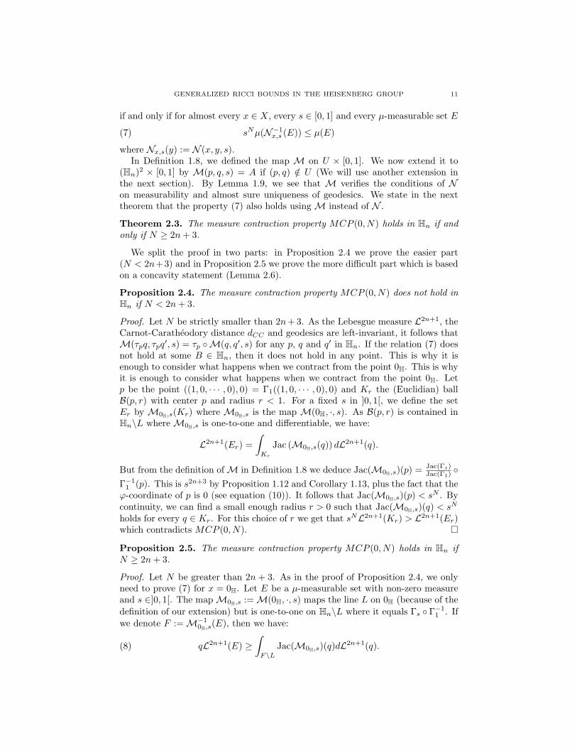
Proposition 2.4. The measure contraction property MCP (0, N) does not hold inHn if N < 2n + 3.

Proof. Let N be strictly smaller than 2n + 3. As the Lebesgue measure L2n+1, theCarnot-Caratheodory distance dCC and geodesics are left-invariant, it follows thatM(τpq, τpq

′, s) = τp ◦M(q, q′, s) for any p, q and q′ in Hn. If the relation (7) doesnot hold at some B ∈ Hn, then it does not hold in any point. This is why it isenough to consider what happens when we contract from the point 0H. This is whyit is enough to consider what happens when we contract from the point 0H. Letp be the point ((1, 0, · · · , 0), 0) = Γ1((1, 0, · · · , 0), 0) and Kr the (Euclidian) ballB(p, r) with center p and radius r < 1. For a fixed s in ]0, 1[, we define the setEr by M0H,s(Kr) where M0H,s is the map M(0H, ·, s). As B(p, r) is contained inHn\L where M0H,s is one-to-one and differentiable, we have:

L2n+1(Er) =∫

Kr

Jac (M0H,s(q)) dL2n+1(q).

But from the definition of M in Definition 1.8 we deduce Jac(M0H,s)(p) = Jac(Γs)Jac(Γ1)

◦Γ−1

1 (p). This is s2n+3 by Proposition 1.12 and Corollary 1.13, plus the fact that theϕ-coordinate of p is 0 (see equation (10)). It follows that Jac(M0H,s)(p) < sN . Bycontinuity, we can find a small enough radius r > 0 such that Jac(M0H,s)(q) < sN

holds for every q ∈ Kr. For this choice of r we get that sNL2n+1(Kr) > L2n+1(Er)which contradicts MCP (0, N). �

Proposition 2.5. The measure contraction property MCP (0, N) holds in Hn ifN ≥ 2n + 3.

Proof. Let N be greater than 2n + 3. As in the proof of Proposition 2.4, we onlyneed to prove (7) for x = 0H. Let E be a µ-measurable set with non-zero measureand s ∈]0, 1[. The map M0H,s := M(0H, ·, s) maps the line L on 0H (because of thedefinition of our extension) but is one-to-one on Hn\L where it equals Γs ◦ Γ−1

1 . Ifwe denote F := M−1

0H,s(E), then we have:

qL2n+1(E) ≥∫

F\LJac(M0H,s)(q)dL2n+1(q).(8)

12 NICOLAS JUILLET

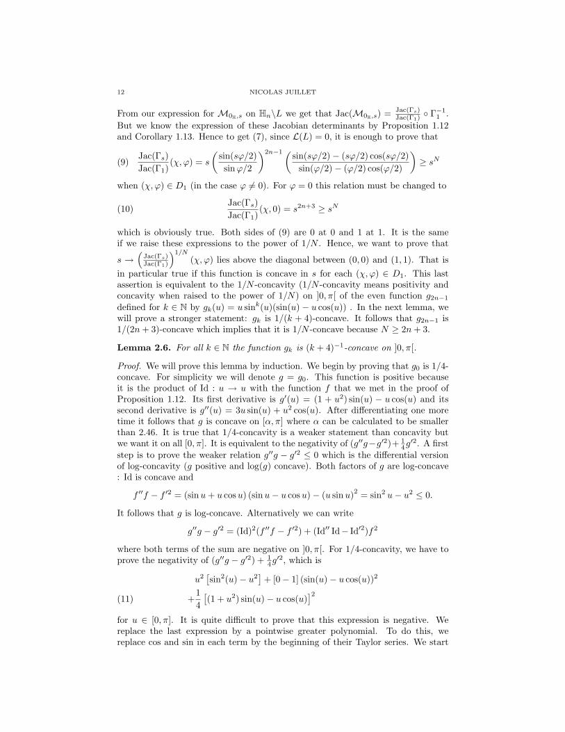
From our expression for M0H,s on Hn\L we get that Jac(M0H,s) = Jac(Γs)Jac(Γ1)

◦ Γ−11 .

But we know the expression of these Jacobian determinants by Proposition 1.12and Corollary 1.13. Hence to get (7), since L(L) = 0, it is enough to prove that

Jac(Γs)Jac(Γ1)

(χ, ϕ) = s

(sin(sϕ/2)sinϕ/2

)2n−1( sin(sϕ/2)− (sϕ/2) cos(sϕ/2)sin(ϕ/2)− (ϕ/2) cos(ϕ/2)

)≥ sN(9)

when (χ, ϕ) ∈ D1 (in the case ϕ 6= 0). For ϕ = 0 this relation must be changed to

Jac(Γs)Jac(Γ1)

(χ, 0) = s2n+3 ≥ sN(10)

which is obviously true. Both sides of (9) are 0 at 0 and 1 at 1. It is the sameif we raise these expressions to the power of 1/N . Hence, we want to prove that

s →(

Jac(Γs)Jac(Γ1)

)1/N

(χ, ϕ) lies above the diagonal between (0, 0) and (1, 1). That isin particular true if this function is concave in s for each (χ, ϕ) ∈ D1. This lastassertion is equivalent to the 1/N -concavity (1/N -concavity means positivity andconcavity when raised to the power of 1/N) on ]0, π[ of the even function g2n−1

defined for k ∈ N by gk(u) = u sink(u)(sin(u) − u cos(u)) . In the next lemma, wewill prove a stronger statement: gk is 1/(k + 4)-concave. It follows that g2n−1 is1/(2n + 3)-concave which implies that it is 1/N -concave because N ≥ 2n + 3.

Lemma 2.6. For all k ∈ N the function gk is (k + 4)−1-concave on ]0, π[.

Proof. We will prove this lemma by induction. We begin by proving that g0 is 1/4-concave. For simplicity we will denote g = g0. This function is positive becauseit is the product of Id : u → u with the function f that we met in the proof ofProposition 1.12. Its first derivative is g′(u) = (1 + u2) sin(u) − u cos(u) and itssecond derivative is g′′(u) = 3u sin(u) + u2 cos(u). After differentiating one moretime it follows that g is concave on [α, π] where α can be calculated to be smallerthan 2.46. It is true that 1/4-concavity is a weaker statement than concavity butwe want it on all [0, π]. It is equivalent to the negativity of (g′′g−g′2)+ 1

4g′2. A firststep is to prove the weaker relation g′′g − g′2 ≤ 0 which is the differential versionof log-concavity (g positive and log(g) concave). Both factors of g are log-concave: Id is concave and

f ′′f − f ′2 = (sinu + u cos u) (sinu− u cos u)− (u sinu)2 = sin2 u− u2 ≤ 0.

It follows that g is log-concave. Alternatively we can write

g′′g − g′2 = (Id)2(f ′′f − f ′2) + (Id′′ Id− Id′2)f2

where both terms of the sum are negative on ]0, π[. For 1/4-concavity, we have toprove the negativity of (g′′g − g′2) + 1

4g′2, which is

u2[sin2(u)− u2

]+ [0− 1] (sin(u)− u cos(u))2

+14[(1 + u2) sin(u)− u cos(u)

]2(11)

for u ∈ [0, π]. It is quite difficult to prove that this expression is negative. Wereplace the last expression by a pointwise greater polynomial. To do this, wereplace cos and sin in each term by the beginning of their Taylor series. We start


with 14g′2(u). It is constructed from g′ which is positive for u ∈ [0, π]. On this

interval, we have:

0 ≤ (1 + u2) sin(u)− u cos(u) ≤ (1 + u2)(u− u3/6 + u5/120)− u(1− u2/2).

For 0 ≤ u ≤ 2√

2, we have

sin(u)− u cos(u) ≥ (u− u3/6)− u(1− u2/2 + u4/24) = u3/3− u5/24 ≥ 0

and finally, for u ∈ [0, π] we have

0 ≤ sin(u) ≤ u− u3/6 + u5/120.

We can then estimate (11) for u ≤ 2√

2:

u2[sin2(u)− u2

]− (sin(u)− u cos(u))2

+14[(1 + u2) sin(u)− u cos(u)

]2=u2

[(u− u3/6 + u5/120)2 − u2

]− (u3/3− u5/24)2

+14((1 + u2)(u− u3/6 + u5/120)− u(1− u2/2))2

=− 130

u8 +421

57600u10 − 17

28800u12 +

157600

u14

≤u8

((8

57600− 17

28800

)(u2)2 +

42157600

u2 − 130

)≤ 0.

So we have 1/4-concavity of g on [0, 2√

2]. But we already proved that g is concaveon [2.46, π]. Thus g is 1/4-concave on [0, π] which is the reunion of the two intervals.

Let us now prove by induction that gk+1 is 1/(k + 5)-concave. For this let usassume that gk is 1/(k + 4)-concave for some integer k. Then gk+1 = gk · sin. Wehave now to prove the negativity of

((gk sin)′′(gk sin)− (gk sin)′2

)+

1k + 5

(gk sin)′2

=(g′′kgk − g′2k ) sin2 +(− sin sin− cos2)g2k +

1k + 5

(gk sin)′2

=(g′′kgk − g′2k ) sin2−g2k +

g′2k sin2 +2gkg′k sin cos +g2k cos2

k + 5

=(g′′kgk − g′2k +g′2k

k + 4) sin2−g′2k sin2

k + 4− g2

k +g′2k sin2 +2gkg′k sin cos +g2

k cos2

k + 5

=(g′′kgk − g′2k +g′2k

k + 4) sin2 +

−g′2k sin2

(k + 4)(k + 5)+ g2

k

(cos2

k + 5− 1)

+2gkg′k sin cos

k + 5.

The first term T1 in the last sum is negative because of the 1/(k + 4)-concavity ofgk. The second term T2 is clearly negative. The third term T3 is also negative. Itremains to prove that |T4| ≤ |T2| + |T3| where T4 is the last term. We compare

14 NICOLAS JUILLET

|T4|2 and (2√|T2||T3|)2 ≤ (|T2|+ |T3|)2:

4|T2||T3| − T 24

=4[

g′2k sin2

(k + 4)(k + 5)

] [g2

k

(1− cos2

k + 5

)]−[2gkg′k sin cos

k + 5

]2=4g2

kg′2k sin2

[k+5−cos2

k+4 − cos2

(k + 5)2

]≥ 0.

�

�

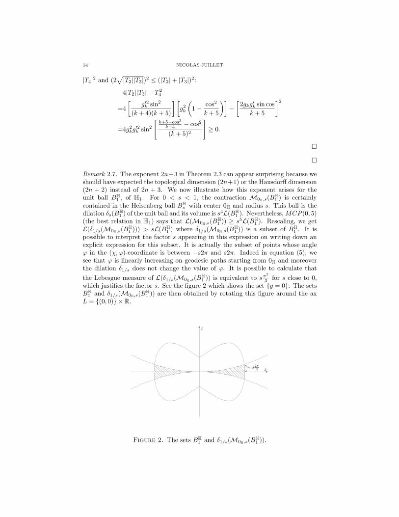
Remark 2.7. The exponent 2n+3 in Theorem 2.3 can appear surprising because weshould have expected the topological dimension (2n+1) or the Hausdorff dimension(2n + 2) instead of 2n + 3. We now illustrate how this exponent arises for theunit ball BH

1 , of H1. For 0 < s < 1, the contraction M0H,s(BH1 ) is certainly

contained in the Heisenberg ball BHs with center 0H and radius s. This ball is the

dilation δs(BH1 ) of the unit ball and its volume is s4L(BH

1 ). Nevertheless, MCP (0, 5)(the best relation in H1) says that L(M0H,s(BH

1 )) ≥ s5L(BH1 ). Rescaling, we get

L(δ1/s(M0H,s(BH1 ))) > sL(BH

1 ) where δ1/s(M0H,s(BH1 )) is a subset of BH

1 . It ispossible to interpret the factor s appearing in this expression on writing down anexplicit expression for this subset. It is actually the subset of points whose angleϕ in the (χ, ϕ)-coordinate is between −s2π and s2π. Indeed in equation (5), wesee that ϕ is linearly increasing on geodesic paths starting from 0H and moreoverthe dilation δ1/s does not change the value of ϕ. It is possible to calculate thatthe Lebesgue measure of L(δ1/s(M0H,s(BH

1 )) is equivalent to sπ2

3 for s close to 0,which justifies the factor s. See the figure 2 which shows the set {y = 0}. The setsBH

1 and δ1/s(M0H,s(BH1 )) are then obtained by rotating this figure around the ax

L = {(0, 0)} × R.

t

x∼ s

2π

3

Figure 2. The sets BH1 and δ1/s(M0H,s(BH

1 )).


Remark 2.8. The measure contraction property MCP (0, 2n + 3) can be directlyapplied to the Heisenberg group Hn in to prove a (1, 1)-Poincare inequality. To dothis we follow the plan given at the end of the book by Saloff-Coste (see [24, 5.6.3])for manifolds with a lower Ricci bound. This can be easily adapted: we obtain aconstant 22n+3/n. For every p ∈ Hn, r > 0 and smooth function f we have:∫

BH(p,r)

|f(q)− fB | dL(q) ≤ 22n+3

nr

∫BH(p,2r)

|∇Hf(q)|H dL(q)

where BH(p, r) is the dCC-ball with center p and radius r, where

fB =1

L(B)

∫BH(p,r)

f(q) dL(q)

and ∇Hf is the Heisenberg gradient defined by

∇Hf =n∑

k=1

(−→Xk · f)

−→Xk + (

−→Y k · f)

−→Y k.

A Poincare inequality on Hn was first proved by Varopoulos in [29].

Remark 2.9. In [10], Figalli and the author use MCP (0, 2n+3) to answer positivelyan open question of Ambrosio and Rigot [1, section 7(c)]. In Hn, the measuresinterpolated by optimal transport between an absolutely continuous measure andan other measure are absolutely continuous as well. As a consequence Pac

2 ⊂ P2,the subspace of absolutely continuous measure is geodesic.

3. The Brunn-Minkowski Inequalities in Hn

The classical Brunn-Minkowski inequality in RN (see [9, 3.2.41] for instance)is a very useful geometric lower bound on the measure of the Minkowski sum (i.ethe usual sum of two sets in RN ) of two compact sets in RN . This inequality isequivalent to the following statement: given two compact sets K0 and K1, in RN

and s ∈ [0, 1] then

(LN )1/N (sK1 + (1− s)K0) ≥ s(LN )1/N (K1) + (1− s)(LN )1/N (K0)

with sK1 + (1− s)K0 = {sk1 + (1− s)k0 ∈ RN | k1 ∈ K1 k0 ∈ K0}. We want togive a meaning to sK1 +(1− s)K0 in a geodesic metric space. For this we considerthe set of the s-intermediate points from a point k0 in K0 to a point k1 in K1. Wecall this set the s-intermediate set and denote it by “sK1 + (1− s)K0”.

Let (X, d, µ) be a metric measure space and N be greater than 1. We say that thegeodesic Brunn-Minkowski inequality BM(0, N) holds in (X, d, µ) if the inequality

µ1/N (“sK1 + (1− s)K0”) ≥ sµ1/N (K1) + (1− s)µ1/N (K0)(12)

is true for every pair compact sets K0 and K1 of non-zero measure. Here µ(“sK1 +(1− s)K0”) will denote the outer measure of “sK1 + (1− s)K0” if the latter is notmeasurable. There is also a “multiplicative” Brunn-Minkowski inequality that hasbeen introduced in the Heisenberg group by Monti in [22] (see also [16]). We dealwith this inequality in Remark 3.5.

Remark 3.1. Let K be a real number and N ≥ 1. The general definition ofCD(K, N) (see [28]) involves a modification of the geometric inequality (6) byfactors roughly depending on the Wasserstein distance between the measures m0

16 NICOLAS JUILLET

and m1. These factors also appear in MCP (K, N) and CD(K, N) in the gener-alization of the inequalities (7) and (12). These three geometric properties have acommon hierarchy when K and N vary: the property for (K, N) implies the prop-erty for (K ′, N) for all K ′ < K. Similarly for a fixed curvature K, the property(K, N) implies the property (K, N ′) for all N ′ > N . Nevertheless a priori thereis no optimal pair (K, N) when the curvature and the dimension both vary (see[23],[28]).

It is proved in [28] that the curvature-dimension property CD(0, N) impliesBM(0, N). In order to prove that CD(0, N) does not hold in Hn, we will provethat no geodesic Brunn-Minkowski inequality holds in this space.

In Hn it will be useful to interpret the s-intermediate set using the intermediate-points map M. To do this we extend M in a way different from that used inthe last section. Here M is no longer a map but a multi-valued map defined on(Hn)2×]0, 1[ by

M(p, q, s) = {ms ∈ Hn | dCC(p, q) =1sdCC(p, ms) =

11− s

dCC(ms, q)}.

If (p, q) is in U , we identify the single-valued set M(p, q, s) with its unique element,which is coherent with Definition 1.8. To get more information on the values takenby M on (Hn)2\U×]0, 1[, it is enough to use Proposition 1.3 and left translations.We will now prove the following lemma:

Lemma 3.2. There are two compact sets K and K ′ such that

L2n+1(K) = L2n+1(K ′) > L2n+1(M1/2(K, K ′))

where M1/2(K, K ′) = {M(k, k′, 1/2) ∈ Hn | k ∈ K and k′ ∈ K ′}.

Let N be a dimension greater than 1. We can raise the inequality in Lemma 3.2to the power 1/N and using (12) we obtain as a corollary the following theorem.

Theorem 3.3. The geodesic Brunn-Minkowski inequality BM(0, N) and the geo-metric curvature-dimension CD(0, N) do not hold for any N .

We now give a proof of Lemma 3.2.

Proof. Let us consider a simple geodesic: the curve of parameter ((1, · · · , 0), 0) onthe interval [−1, 1]. As 2 ·0 < 2π Corollary 1.6 says that this is the unique geodesicdefined on [−1, 1] from p′ = (−1, 0, · · · , 0) to p = (1, 0, · · · , 0): the points p and p′

are I-conjugate and have midpoint 0H. Actually M1/2 := M(·, ·, 1/2) is simply themidpoint map. On U this map is single and is directly defined by setting s = 1/2in Definition 1.8:

M1/2(q′, q) = τq′ ◦ Γ1/2 ◦ Γ−11 ◦ τq′−1(q).(13)

We will now use the geodesic-inversion map introduced in the first section. We recallthat Lemma 1.11 exactly tells us exactly when the midpoint of two I-conjugatepoints in U is 0H. For p and p′ this is the case so p and p′ are in the open setΓ1(D1/2). Our counterexample consists of a small compact ball Kr := B(p, r) withcenter p and (Euclidian) radius r and K ′

r = I(Kr): we then consider the set ofmidpoints between Kr and K ′

r. By continuity we can choose r small enough suchthat Kr ⊂ Γ1(D1/2) and Kr ×K ′

r ⊂ U .We have to show that K ′

r has the same measure as Kr and this measure is greaterthan the measure of M1/2(Kr,K

′r). The first claim is actually straightforward: Γ1


and Γ−1 are diffeomorphisms between the same sets (Proposition 1.7) and have thesame Jacobian determinant up to sign (Corollary 1.13). Hence

L2n+1(K ′r) = L2n+1(Γ−1(Γ−1

1 (Kr))) = L2n+1(Γ1(Γ−11 (Kr))) = L2n+1(Kr).

The key to the second claim is the fact that

M1/2(K ′r,Kr) =

⋃a,b∈Kr

M1/2(I(a), b) =⋃

a,b∈Kr

M1/2(I(a), a + (b− a)).(14)

As Kr ⊂ Γ1(D1/2), Lemma 1.11 shows that if a ∈ Kr, then M1/2(I(a), a) =0H. Therefore the mid-set M1/2(K ′

r,Kr) has very small measure. We will usedifferentiation tools to quantify this idea. By Lemma 1.9, M1/2 is C∞-differentiableon U . For any q ∈ Hn\L let M1/2

q be the map M(q, ·, 1/2). We now write

M1/2(I(a), a + (b− a))(15)

=0 + DM1/2I(a)(a).(b− a)

+[M1/2 (I(a), a + (b− a))−DM1/2

I(a)(a).(b− a)]

=DM1/2p′ (p).(b− a) +

[(DM1/2

I(a)(a)−DM1/2p′ (p)

).(b− a)

]+[M1/2 (I(a), a + (b− a))−DM1/2

I(a)(a).(b− a)].

For a and b close to p, the two last terms of the last sum are small and canbe bounded using the smoothness of M in the differential calculus of R2n+1 (seeLemma 1.9): when r tends to zero,

supa,b∈Kr

∣∣∣(DM1/2I(a)(a)−DM1/2

p′ (p))

.(b− a)

+ M1/2(I(a), a + (b− a))−DM1/2I(a)(a).(b− a)

∣∣∣ = o(r).

Therefore, as Kr − Kr = {q ∈ R2n+1 | q = b − a a, b ∈ B(p, r)} = B(0, 2r), therelations (14) and (15) give the following set inclusion

M1/2(K ′r,Kr) ⊂ DM1/2

p′ (p).(B(0, 2r)) + B(0, ε(r)r)(16)

where ε(r) is a non-negative function which tends to zero when r tends to zero. Weobserve now that the measure of the right-hand set is equivalent to the measure ofDM1/2

p′ (p).(B(0, 2r)). Considering relation (13) and recalling that the left-invariantaffine maps τp′ and τp′−1 = τ−1

p′ have derivative equal to their linear part, we get

that Jac(M1/2p′ )(p) has the same value as Jac(Γ1/2 ◦Γ−1

1 ) taken at the point p′−1 · pwhich is ((2, 0, · · · , 0), 0) = Γ1((2, 0, · · · , 0), 0). This Jacobian determinant wascalculated in the second section (see equations (9) and (10)). In our case as theϕ-coordinate of Γ−1

1 (p′−1 · p) is 0, we have to use equation (10) for s = 1/2. Thevalue of the Jacobian determinant is then 1

22n+3 . It follows that

L2n+1(DM1/2p′ (p).(B(0, 2r))) =

22n+1

22n+3L2n+1(B(p, r)) =

14L2n+1(Kr).

Hence by (16) and the remark that follows it, we get that

L2n+1(M1/2(K ′r,Kr)) ≤

14L2n+1(Kr)(1 + o(r))

when r tends to zero. We now choose a small enough r and the lemma is proved. �

18 NICOLAS JUILLET

Remark 3.4. (i) The previous result does not only yields that CD(0, N) doesnot hold. This also implies that CD(K, N) does not hold for any K > 0because this condition is less demanding than CD(0, N). Alternatively,spaces verifying CD(K, N) with K > 0 are bounded.

(ii) Also for any K < 0, the curvature-dimension bound CD(K, N) does nothold. We argue by contradiction. Assume that CD(K, N) holds in thespace (Hn, dCC ,L2n+1) for K < 0. Then the “scaled space” property from[28] tells us that (Hn, λ−1dCC , λ−(2n+2)L2n+1) verifies CD(λ2K, N) for allλ > 0. But this last space is exactly isomorphic to our metric measure spacevia the dilation δλ. Hence CD(K ′, N) would hold in (Hn, dCC ,L2n+1) forevery non-positive K ′. It is proved in [1] that the optimal transport betweentwo measures is unique, so inequality (6) defining CD(0, N) is obtained aslimit of the corresponding inequalities for CD(K ′, N), which contradictsTheorem 3.3. It follows that CD(K, N) does not hold in Hn.

(iii) In the same way, we could have proved directly that BM(K, N) is false forany K ∈ R using the dilations of Hn. It follows that CD(K, N) does nothold because CD(K, N) implies BM(K, N).

(iv) The property CD(K, +∞) is defined in [27]. With the same argument as(ii) it implies CD(0,+∞). This property implies the Brunn-Minkowskiinequality (1− s) ln(L(K0)) + s ln(L(K1)) ≤ ln(L(Ms(K0,K1))). It is alsofalse because of Lemma 3.2.

(iv) For every N , the measure contraction property MCP (K, N) is false forK > 0. As for CD, the spaces verifying this condition are bounded (see[28]).

(vi) The property MCP (K, N) also does not hold for N > 2n + 3 and K < 0.This case is similar to (ii): using dilations we can show that MCP (K, N)implies MCP (0, N), which contradicts Theorem 2.3.

Remark 3.5. In [22], Monti compares the measure of two compact sets F and F ′

to the measure of F · F ′ = {a · b ∈ Hn | a ∈ F b ∈ F ′}. He proves that

L3(F · F ′)1/4 ≥ L3(F )1/4 + L3(F ′)1/4

does not hold in H1 (4 is the Hausdorff dimension of H1) using an argument basedon the non-optimality of the unit ball in the isoperimetric inequality for H1.

Another proof for Hn of Hausdorff dimension 2n + 2 is the following: Take F tobe the set Kr defined above and denote by F ′ the set {b ∈ Hn | ∃c ∈ F, c·b = 0H} ofinverse elements (it is simply −F because (z, t)−1 = (−z,−t)). Using the methodsof this section we get that F · F ′ is very close to Dτp′(p).(B(0, 2r)). The measureof this last set is 22n+1L(F ) because, as we said in the first section, Jac(τp′) = 1 inevery point. As L2n+1(F ) = L2n+1(F ′) it follows that for r small enough

L2n+1(F · F ′)1

2n+2 < L2n+1(F )1

2n+2 + L2n+1(F ′)1

2n+2(17)

and the multiplicative Brunn-Minkowski inequality is false for Hausdorff dimension(i.e. 2n+2). In the paper by Leonardi and Masnou (see [16]), the authors show thatthe multiplicative Brunn-Minkowski inequality is true with topological dimension(i.e. 2n + 1). They explain that there could be in principle an N ∈]2n + 1, 2n + 2[such that the multiplicative Brunn-Minkowski inequality holds in Hn: in fact if thisequality holds for N , then it holds for N ′ < N . On the other hand, as mentionedin Remark 3.4, BM(K, N ′) is a consequence of BM(K, N) if N ′ > N .


We proved in (17) that the sets F and F ′ defined in this remark are a counterex-ample to the multiplicative Brunn-Minkowski inequality with dimension N = 2n+2.They are actually also counterexamples for any N > 2n + 1. It follows that 2n + 1is the largest dimension for which the multiplicative Brunn-Minkowski inequalityis true.

Implication Graph

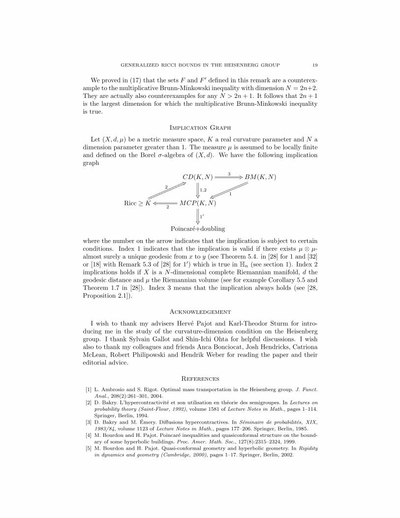
Let (X, d, µ) be a metric measure space, K a real curvature parameter and N adimension parameter greater than 1. The measure µ is assumed to be locally finiteand defined on the Borel σ-algebra of (X, d). We have the following implicationgraph

CD(K, N) 3 +3

1,2

��

BM(K, N)

1rz llllllllllll

llllllllllll

Ricc ≥ K

2

2:mmmmmmmmmmmmm

mmmmmmmmmmmmmMCP (K, N)

2ks

1′

��Poincare+doubling

where the number on the arrow indicates that the implication is subject to certainconditions. Index 1 indicates that the implication is valid if there exists µ ⊗ µ-almost surely a unique geodesic from x to y (see Theorem 5.4. in [28] for 1 and [32]or [18] with Remark 5.3 of [28] for 1′) which is true in Hn (see section 1). Index 2implications holds if X is a N -dimensional complete Riemannian manifold, d thegeodesic distance and µ the Riemannian volume (see for example Corollary 5.5 andTheorem 1.7 in [28]). Index 3 means that the implication always holds (see [28,Proposition 2.1]).

Acknowledgement

I wish to thank my advisers Herve Pajot and Karl-Theodor Sturm for intro-ducing me in the study of the curvature-dimension condition on the Heisenberggroup. I thank Sylvain Gallot and Shin-Ichi Ohta for helpful discussions. I wishalso to thank my colleagues and friends Anca Bonciocat, Josh Hendricks, CatrionaMcLean, Robert Philipowski and Hendrik Weber for reading the paper and theireditorial advice.

References

[1] L. Ambrosio and S. Rigot. Optimal mass transportation in the Heisenberg group. J. Funct.Anal., 208(2):261–301, 2004.

[2] D. Bakry. L’hypercontractivite et son utilisation en theorie des semigroupes. In Lectures onprobability theory (Saint-Flour, 1992), volume 1581 of Lecture Notes in Math., pages 1–114.Springer, Berlin, 1994.

[3] D. Bakry and M. Emery. Diffusions hypercontractives. In Seminaire de probabilites, XIX,1983/84, volume 1123 of Lecture Notes in Math., pages 177–206. Springer, Berlin, 1985.

[4] M. Bourdon and H. Pajot. Poincare inequalities and quasiconformal structure on the bound-ary of some hyperbolic buildings. Proc. Amer. Math. Soc., 127(8):2315–2324, 1999.

[5] M. Bourdon and H. Pajot. Quasi-conformal geometry and hyperbolic geometry. In Rigidityin dynamics and geometry (Cambridge, 2000), pages 1–17. Springer, Berlin, 2002.

20 NICOLAS JUILLET

[6] D. Burago, Y. Burago, and S. Ivanov. A course in metric geometry, volume 33 of GraduateStudies in Mathematics. American Mathematical Society, Providence, RI, 2001.

[7] J. Cheeger. Differentiability of Lipschitz functions on metric measure spaces. Geom. Funct.Anal., 9(3):428–517, 1999.

[8] D. Cordero-Erausquin, R. J. McCann, and M. Schmuckenschlager. A Riemannian interpola-tion inequality a la Borell, Brascamp and Lieb. Invent. Math., 146(2):219–257, 2001.

[9] H. Federer. Geometric measure theory. Die Grundlehren der mathematischen Wissenschaften,Band 153. Springer-Verlag New York Inc., New York, 1969.

[10] A. Figalli and N. Juillet. Absolute continuity of Wasserstein geodesics in the Heisenberggroup. J. Funct. Anal., 255(1):133–141, 2008.

[11] B. Gaveau. Principe de moindre action, propagation de la chaleur et estimees sous elliptiquessur certains groupes nilpotents. Acta Math., 139(1-2):95–153, 1977.

[12] P. Haj lasz and P. Koskela. Sobolev met Poincare. Mem. Amer. Math. Soc., 145(688):x+101,2000.

[13] J. Heinonen. Lectures on analysis on metric spaces. Universitext. Springer-Verlag, New York,2001.

[14] T. J. Laakso. Ahlfors Q-regular spaces with arbitrary Q > 1 admitting weak Poincare in-equality. Geom. Funct. Anal., 10(1):111–123, 2000.

[15] T. J. Laakso. Erratum to: “Ahlfors Q-regular spaces with arbitrary Q > 1 admittingweak Poincare inequality” [Geom. Funct. Anal. 10 (2000), no. 1, 111–123; MR1748917(2001m:30027)]. Geom. Funct. Anal., 12(3):650, 2002.

[16] G. P. Leonardi and S. Masnou. On the isoperimetric problem in the Heisenberg group Hn.Ann. Mat. Pura Appl. (4), 184(4):533–553, 2005.

[17] J. Lott and C. Villani. Ricci curvature for metric-measure spaces via optimal transport. toappear in Ann of Math., 2006.

[18] J. Lott and C. Villani. Weak curvature conditions and functional inequalities. J. Funct. Anal.,245(1):311–333, 2007.

[19] R. J. McCann. Polar factorization of maps on Riemannian manifolds. Geom. Funct. Anal.,11(3):589–608, 2001.

[20] R. Montgomery. A tour of subriemannian geometries, their geodesics and applications, vol-ume 91 of Mathematical Surveys and Monographs. American Mathematical Society, Provi-dence, RI, 2002.

[21] R. Monti. Some properties of Carnot-Caratheodory balls in the Heisenberg group. Atti Accad.Naz. Lincei Cl. Sci. Fis. Mat. Natur. Rend. Lincei (9) Mat. Appl., 11(3):155–167 (2001),2000.

[22] R. Monti. Brunn-Minkowski and isoperimetric inequality in the Heisenberg group. Ann. Acad.Sci. Fenn. Math., 28(1):99–109, 2003.

[23] S.-I. Ohta. On the measure contraction property of metric measure spaces. Comment. Math.Helv., 82(4):805–828, 2007.

[24] L. Saloff-Coste. Aspects of Sobolev-type inequalities, volume 289 of London MathematicalSociety Lecture Note Series. Cambridge University Press, Cambridge, 2002.

[25] S. Semmes. An introduction to Heisenberg groups in analysis and geometry. Notices Amer.Math. Soc., 50(6):640–646, 2003.

[26] N. Shanmugalingam. Newtonian spaces: an extension of Sobolev spaces to metric measurespaces. Rev. Mat. Iberoamericana, 16(2):243–279, 2000.

[27] K.-T. Sturm. On the geometry of metric measure spaces. I. Acta Math., 196(1):65–131, 2006.[28] K.-T. Sturm. On the geometry of metric measure spaces. II. Acta Math., 196(1):133–177,

2006.[29] N. T. Varopoulos. Fonctions harmoniques sur les groupes de Lie. C. R. Acad. Sci. Paris Ser.

I Math., 304(17):519–521, 1987.[30] C. Villani. Topics in optimal transportation, volume 58 of Graduate Studies in Mathematics.

American Mathematical Society, Providence, RI, 2003.[31] C. Villani. Optimal transport, old and new. Springer (to appear in Grundlehren der mathe-

matischen Wissenschaften), 2008.[32] M.-K. von Renesse. On local Poincare via transportation. Math. Z., 259(1):21–31, 2008.


Institut Fourier BP 74, UMR 5582, Universite Grenoble I, 38402 Saint-Martin-d’HeresCedex, France

E-mail address: [email protected]

Institut fur Angewandte Mathematik, Universitat Bonn, Poppelsdorfer Allee 82,53115 Bonn, Germany

E-mail address: [email protected]

geometric inequalities and generalized ricci bounds...

Documents