5

Gravity

5.1 Introduction

The force exerted on an element of mass at the surface of the Earth has twoprincipal components. One is due to the gravitational attraction of the massin the Earth, and the other is due to the rotation of the Earth. Gravity refersto the combined effects of both gravitation and rotation. If the Earth werea nonrotating spherically symmetric body, the gravitational acceleration onits surface would be constant. However, because of the Earth’s rotation,topography, and internal lateral density variations, the acceleration of gravityg varies with location on the surface. The Earth’s rotation leads mainly to alatitude dependence of the surface acceleration of gravity. Because rotationdistorts the surface by producing an equatorial bulge and a polar flattening,gravity at the equator is about 5 parts in 1000 less than gravity at the poles.The Earth takes the shape of an oblate spheroid. The gravitational field ofthis spheroid is the reference gravitational field of the Earth. Topographyand density inhomogeneities in the Earth lead to local variations in thesurface gravity, which are referred to as gravity anomalies.

The mass of the rock associated with topography leads to surface gravityanomalies. However, as we discussed in Chapter 2, large topographic featureshave low-density crustal roots. Just as the excess mass of the topographyproduces a positive gravity anomaly, the low-density root produces a nega-tive gravity anomaly. In the mid-1800s it was observed that the gravitationalattraction of the Himalayan Mountains was considerably less than would beexpected because of the positive mass of the topography. This was the firstevidence that the crust–mantle boundary is depressed under large mountainbelts.

A dramatic example of the importance of crustal thickening is the ab-sence of positive gravity anomalies over the continents. The positive mass

5.2 Gravitational Acceleration 355

anomaly associated with the elevation of the continents above the oceanfloor is reduced or compensated by the negative mass anomaly associatedwith the thicker continental crust. We will show that compensation due tothe hydrostatic equilibrium of thick crust leads in the first approximationto a zero value for the surface gravity anomaly. There are mechanisms forcompensation other than the simple thickening of the crust. An exampleis the subsidence of the ocean floor due to the thickening of the thermallithosphere, as discussed in Section 4–23.

Gravity anomalies that are correlated with topography can be used tostudy the flexure of the elastic lithosphere under loading. Short wavelengthloads do not depress the lithosphere, but long wavelength loads result inflexure and a depression of the Moho. Gravity anomalies can also have im-portant economic implications. Ore minerals are usually more dense than thecountry rock in which they are found. Therefore, economic mineral depositsare usually associated with positive gravity anomalies. Major petroleum oc-currences are often found beneath salt domes. Since salt is less dense thanother sedimentary rocks, salt domes are usually associated with negativegravity anomalies.

As we will see in the next chapter, mantle convection is driven by vari-ations of density in the Earth’s mantle. These variations produce grav-ity anomalies at the Earth’s surface. Thus, measurements of gravity atthe Earth’s surface can provide important constraints on the flow patternswithin the Earth’s interior. However, it must be emphasized that the surfacegravity does not provide a unique measure of the density distribution withinthe Earth’s interior. Many different internal density distributions can givethe same surface distributions of gravity anomalies. In other words, inver-sions of gravity data are non-unique.

5.2 Gravitational Acceleration External to the RotationallyDistorted Earth

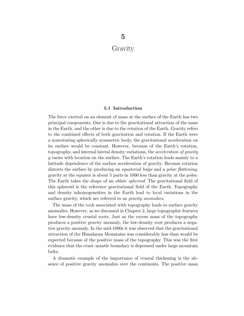
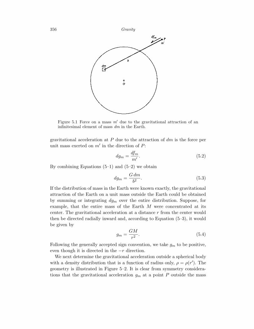
The gravitational force exerted on a mass m′ located at point P outside theEarth by a small element of mass dm in the Earth is given by Newton’s lawof gravitation. As shown in Figure 5–1, the gravitational attraction dfm inthe direction from P to dm is given by

dfm =Gm′dm

b2, (5.1)

where G is the universal gravitational constant G = 6.673 × 10−11 m3 kg−1

s−2 and b is the distance between dm and the point P . The infinitesimal

356 Gravity

Figure 5.1 Force on a mass m′ due to the gravitational attraction of aninfinitesimal element of mass dm in the Earth.

gravitational acceleration at P due to the attraction of dm is the force perunit mass exerted on m′ in the direction of P :

dgm =dfm

m′. (5.2)

By combining Equations (5–1) and (5–2) we obtain

dgm =Gdm

b2. (5.3)

If the distribution of mass in the Earth were known exactly, the gravitationalattraction of the Earth on a unit mass outside the Earth could be obtainedby summing or integrating dgm over the entire distribution. Suppose, forexample, that the entire mass of the Earth M were concentrated at itscenter. The gravitational acceleration at a distance r from the center wouldthen be directed radially inward and, according to Equation (5–3), it wouldbe given by

gm =GM

r2. (5.4)

Following the generally accepted sign convention, we take gm to be positive,even though it is directed in the −r direction.

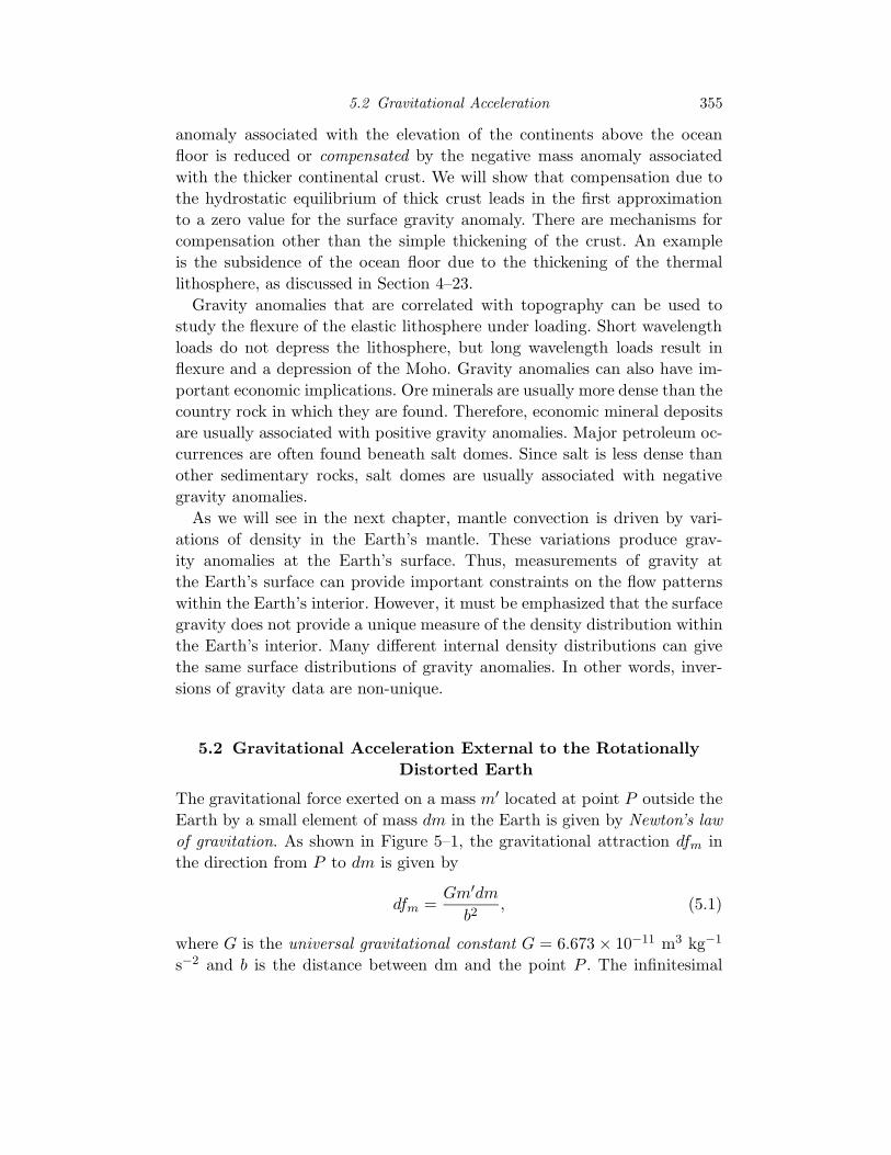
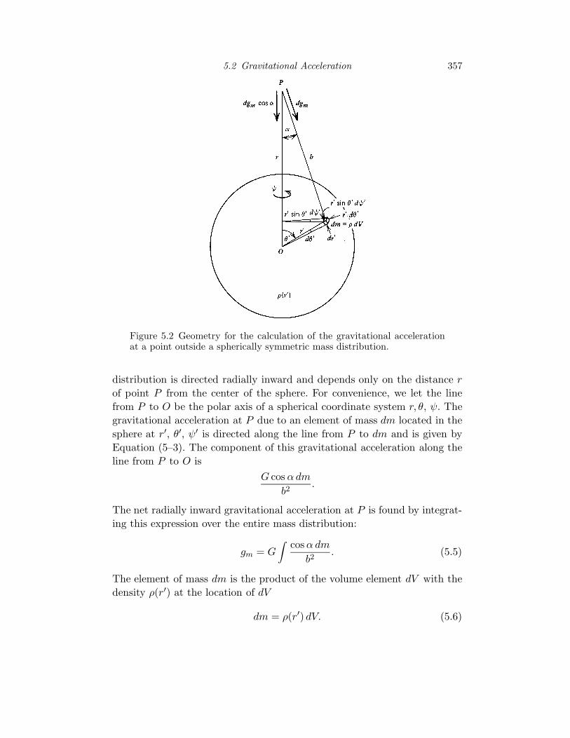
We next determine the gravitational acceleration outside a spherical bodywith a density distribution that is a function of radius only, ρ = ρ(r′). Thegeometry is illustrated in Figure 5–2. It is clear from symmetry considera-tions that the gravitational acceleration gm at a point P outside the mass

5.2 Gravitational Acceleration 357

Figure 5.2 Geometry for the calculation of the gravitational accelerationat a point outside a spherically symmetric mass distribution.

distribution is directed radially inward and depends only on the distance rof point P from the center of the sphere. For convenience, we let the linefrom P to O be the polar axis of a spherical coordinate system r, θ, ψ. Thegravitational acceleration at P due to an element of mass dm located in thesphere at r′, θ′, ψ′ is directed along the line from P to dm and is given byEquation (5–3). The component of this gravitational acceleration along theline from P to O is

G cosα dm

b2.

The net radially inward gravitational acceleration at P is found by integrat-ing this expression over the entire mass distribution:

gm = G!

cosα dm

b2. (5.5)

The element of mass dm is the product of the volume element dV with thedensity ρ(r′) at the location of dV

dm = ρ(r′) dV. (5.6)

358 Gravity

The element of volume can be expressed in spherical coordinates as

dV = r′2 sin θ′ dθ′ dψ′ dr′. (5.7)

The integral over the spherical mass distribution in Equation (5–5) can thusbe written

gm = G! a

0

! π

0

! 2π

0

ρ(r′)r′2 sin θ′ cosα dψ′ dθ′ dr′

b2,

(5.8)

where a is the radius of the model Earth. The integral over ψ′ is 2π, sincethe quantities in the integrand of Equation (5–8) are independent of ψ′. Tocarry out the integration over r′ and θ′, we need an expression for cosα.From the law of cosines we can write

cosα =b2 + r2 − r′2

2rb. (5.9)

Because the expression for cos α involves b rather than θ′, it is more conve-nient to rewrite Equation (5–8) so that the integration can be carried outover b rather than over θ′. The law of cosines can be used again to find anexpression for cos θ′:

cos θ′ =r′2 + r2 − b2

2rr′. (5.10)

By differentiating Equation (5–10) with r and r′ held constant, we find

sin θ′dθ′ =b db

rr′. (5.11)

Upon substitution of Equations (5–9) and (5–11) into Equation (5–8), wecan write the integral expression for gm as

gm =πG

r2

! a

0r′ρ(r′)

! r+r′

r−r′

"

r2 − r′2

b2+ 1

#

db dr′.

(5.12)

The integration over b gives 4 r′ so that Equation (5–12) becomes

gm =4πG

r2

! a

0dr′r′2ρ(r′). (5.13)

Since the total mass of the model is given by

M = 4π! a

0dr′r′2ρ(r′), (5.14)

5.2 Gravitational Acceleration 359

the gravitational acceleration is

gm =GM

r2. (5.15)

The gravitational acceleration of a spherically symmetric mass distribu-tion, at a point outside the mass, is identical to the acceleration obtainedby concentrating all the mass at the center of the distribution. Even thoughthere are lateral density variations in the Earth and the Earth’s shape is dis-torted by rotation, the direction of the gravitational acceleration at a pointexternal to the Earth is very nearly radially inward toward the Earth’s cen-ter of mass, and Equation (5–15) provides an excellent first approximationfor gm.

Problem 5.1 For a point on the surface of the Moon determine the ratioof the acceleration of gravity due to the mass of the Earth to the accelerationof gravity due to the mass of the Moon.

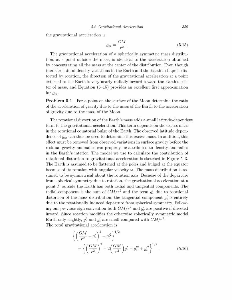
The rotational distortion of the Earth’s mass adds a small latitude-dependentterm to the gravitational acceleration. This term depends on the excess massin the rotational equatorial bulge of the Earth. The observed latitude depen-dence of gm can thus be used to determine this excess mass. In addition, thiseffect must be removed from observed variations in surface gravity before theresidual gravity anomalies can properly be attributed to density anomaliesin the Earth’s interior. The model we use to calculate the contribution ofrotational distortion to gravitational acceleration is sketched in Figure 5–3.The Earth is assumed to be flattened at the poles and bulged at the equatorbecause of its rotation with angular velocity ω. The mass distribution is as-sumed to be symmetrical about the rotation axis. Because of the departurefrom spherical symmetry due to rotation, the gravitational acceleration at apoint P outside the Earth has both radial and tangential components. Theradial component is the sum of GM/r2 and the term g′r due to rotationaldistortion of the mass distribution; the tangential component g′t is entirelydue to the rotationally induced departure from spherical symmetry. Follow-ing our previous sign convention both GM/r2 and g′r are positive if directedinward. Since rotation modifies the otherwise spherically symmetric modelEarth only slightly, g′r and g′t are small compared with GM/r2.The total gravitational acceleration is

"$

GM

r2+ g′r

%2

+ g′2t

#1/2

="$

GM

r2

%2

+ 2$

GM

r2

%

g′r + g′2r + g′2t

#1/2

. (5.16)

360 Gravity

Figure 5.3 Geometry for calculating the contribution of rotational distor-tion to the gravitational acceleration.

It is appropriate to neglect the quadratic terms because the magnitudes of g′rand g′t are much less than GM/r2. Therefore the gravitational accelerationis given by

"$

GM

r2

%2

+ 2$

GM

r2

%

g′r

#1/2

=$

GM

r2

%"

1 +2g′r

GM/r2

#1/2

=$

GM

r2

%"

1 +g′r

GM/r2

#

=GM

r2+ g′r. (5.17)

Equation (5–17) shows that the tangential component of the gravitationalacceleration is negligible; the net gravitational acceleration at a point Pexternal to a rotationally distorted model Earth is essentially radially inwardto the center of the mass distribution.

The radial gravitational acceleration for the rotationally distorted Earthmodel can be obtained by integrating Equation (5–5) over the entire massdistribution. We can rewrite this equation for gm by substituting expression(5–9) for cos α with the result

gm =G

2r2

!"

r

b+

r3

b3

$

1 −r′2

r2

%#

dm. (5.18)

5.2 Gravitational Acceleration 361

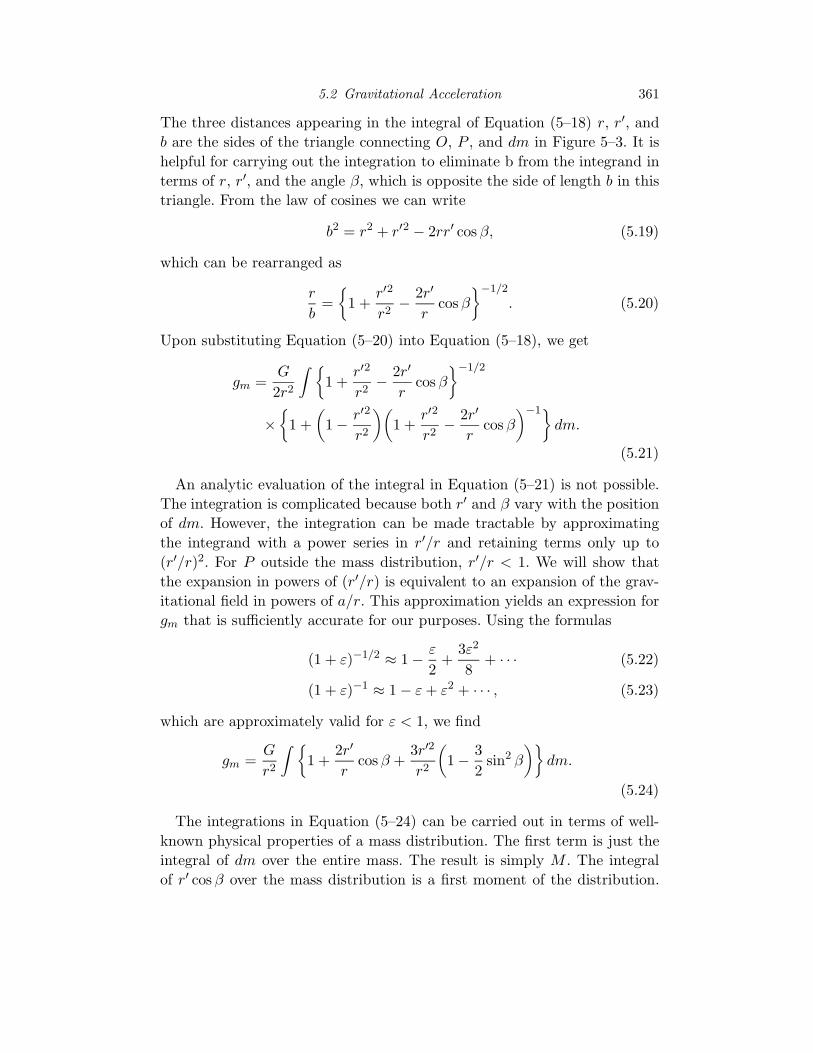
The three distances appearing in the integral of Equation (5–18) r, r′, andb are the sides of the triangle connecting O, P , and dm in Figure 5–3. It ishelpful for carrying out the integration to eliminate b from the integrand interms of r, r′, and the angle β, which is opposite the side of length b in thistriangle. From the law of cosines we can write

b2 = r2 + r′2 − 2rr′ cos β, (5.19)

which can be rearranged as

r

b="

1 +r′2

r2−

2r′

rcos β

#−1/2

. (5.20)

Upon substituting Equation (5–20) into Equation (5–18), we get

gm =G

2r2

!"

1 +r′2

r2−

2r′

rcos β

#−1/2

×"

1 +$

1 −r′2

r2

%$

1 +r′2

r2−

2r′

rcos β

%−1#

dm.

(5.21)

An analytic evaluation of the integral in Equation (5–21) is not possible.The integration is complicated because both r′ and β vary with the positionof dm. However, the integration can be made tractable by approximatingthe integrand with a power series in r′/r and retaining terms only up to(r′/r)2. For P outside the mass distribution, r′/r < 1. We will show thatthe expansion in powers of (r′/r) is equivalent to an expansion of the grav-itational field in powers of a/r. This approximation yields an expression forgm that is sufficiently accurate for our purposes. Using the formulas

(1 + ε)−1/2 ≈ 1 −ε

2+

3ε2

8+ · · · (5.22)

(1 + ε)−1 ≈ 1 − ε+ ε2 + · · · , (5.23)

which are approximately valid for ε < 1, we find

gm =G

r2

!"

1 +2r′

rcos β +

3r′2

r2

$

1 −3

2sin2 β

%#

dm.

(5.24)

The integrations in Equation (5–24) can be carried out in terms of well-known physical properties of a mass distribution. The first term is just theintegral of dm over the entire mass. The result is simply M . The integralof r′ cos β over the mass distribution is a first moment of the distribution.

362 Gravity

It is by definition zero if the origin of the coordinate system is the center ofmass of the distribution. Thus Equation (5–24) becomes

gm =GM

r2+

3G

r4

!

r′2$

1 −3

2sin2 β

%

dm. (5.25)

The first term on the right of Equation (5–25) is the gravitational acceler-ation of a spherically symmetric mass distribution. The second term is themodification due to rotationally induced oblateness of the body. If higherorder terms in Equations (5–24) and (5–23) had been retained, the expan-sion given in Equation (5–25) would have been extended to include termsproportional to r−5 and higher powers of r−1.

We will now express the integral appearing in Equation (5–25) in termsof the moments of inertia of an axisymmetric body. We take C to be themoment of inertia of the body about the rotational or z axis defined by θ = 0.This moment of inertia is the integral over the entire mass distribution ofdm times the square of the perpendicular distance from dm to the rotationalaxis. The square of this distance is x′2 + y′2 so that we can write C as

C ≡!

(x′2 + y′2) dm =!

r′2 sin2 θ′ dm (5.26)

because

x′ = r′ sin θ′ cosψ′ (5.27)

y′ = r′ sin θ′ sinψ′. (5.28)

The moment of inertia about the x axis, which is defined by θ = π/2, ψ = 0,is

A ≡!

(y′2 + z ′2) dm

=!

r′2(sin2 θ′ sin2 ψ′ + cos2 θ′) dm (5.29)

because

z′ = r′ cos θ′. (5.30)

Similarly, the moment of inertia about the y axis, which is defined by θ =π/2, ψ = π/2, is

B ≡!

(x′2 + z ′2) dm

=!

r′2(sin2 θ′ cos2 ψ′ + cos2 θ′) dm. (5.31)

5.2 Gravitational Acceleration 363

For a body that is axisymmetric about the rotation or z axis, A = B. Theaddition of Equations (5–26), (5–29), and (5–31) together with the assump-tion of axisymmetry gives

A + B + C = 2!

r′2 dm = 2A + C. (5.32)

This equation expresses the integral of r′2dm appearing in Equation (5–25)in terms of the moments of inertia of the body.

We will next derive an expression for the integral of r′2 sin2 βdm. Becauseof the axial symmetry of the body there is no loss of generality in lettingthe line OP in Figure 5–3 lie in the xz plane. With the help of Equation(5–32) we rewrite the required integral as

!

r′2 sin2 β dm =!

r′2(1 − cos2 β) dm

= A +1

2C −

!

r′2 cos2 β dm.

(5.33)

The quantity r′ cos β is the projection of r′ along OP . But this is also

r′ cos β = x′ cos φ+ z′ sinφ, (5.34)

where φ is the latitude or the angle between OP and the xy plane. Note thaty′ has no projection onto OP , since OP is in the xz plane. We use Equation(5–34) to rewrite the integral of r′2 cos2 β in the form

!

r′2 cos2 β dm = cos2 φ!

x′2 dm

+ sin2 φ!

z ′2 dm

+2cosφ sinφ!

x′z′ dm. (5.35)

For an axisymmetric body,!

x′2 dm =!

y′2 dm. (5.36)

This result and Equation (5–26) give!

x′2 dm =1

2

!

(x′2 + y′2) dm =1

2C. (5.37)

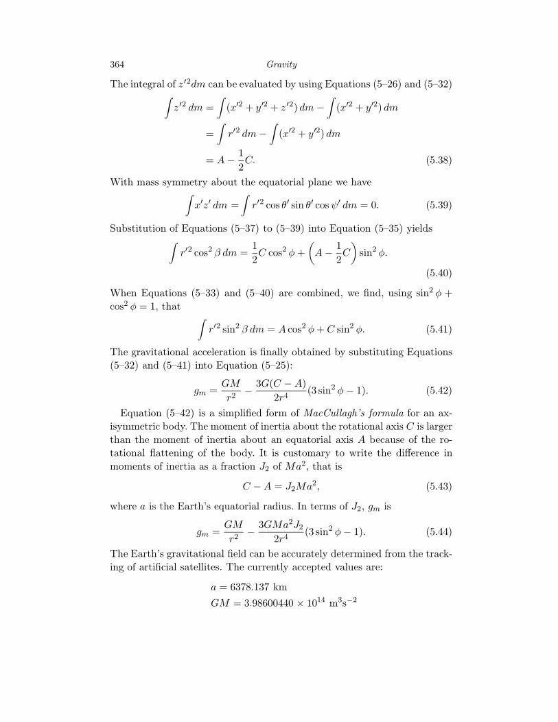
364 Gravity

The integral of z ′2dm can be evaluated by using Equations (5–26) and (5–32)!

z ′2 dm =!

(x′2 + y′2 + z ′2) dm −!

(x′2 + y′2) dm

=!

r′2 dm −!

(x′2 + y′2) dm

= A −1

2C. (5.38)

With mass symmetry about the equatorial plane we have!

x′z′ dm =!

r′2 cos θ′ sin θ′ cosψ′ dm = 0. (5.39)

Substitution of Equations (5–37) to (5–39) into Equation (5–35) yields!

r′2 cos2 β dm =1

2C cos2 φ+

$

A −1

2C%

sin2 φ.

(5.40)

When Equations (5–33) and (5–40) are combined, we find, using sin2 φ +cos2 φ = 1, that

!

r′2 sin2 β dm = A cos2 φ+ C sin2 φ. (5.41)

The gravitational acceleration is finally obtained by substituting Equations(5–32) and (5–41) into Equation (5–25):

gm =GM

r2−

3G(C − A)

2r4(3 sin2 φ− 1). (5.42)

Equation (5–42) is a simplified form of MacCullagh’s formula for an ax-isymmetric body. The moment of inertia about the rotational axis C is largerthan the moment of inertia about an equatorial axis A because of the ro-tational flattening of the body. It is customary to write the difference inmoments of inertia as a fraction J2 of Ma2, that is

C − A = J2Ma2, (5.43)

where a is the Earth’s equatorial radius. In terms of J2, gm is

gm =GM

r2−

3GMa2J2

2r4(3 sin2 φ− 1). (5.44)

The Earth’s gravitational field can be accurately determined from the track-ing of artificial satellites. The currently accepted values are:

a = 6378.137 km

GM = 3.98600440 × 1014 m3s−2

5.3 Centrifugal Acceleration and the Acceleration of Gravity 365

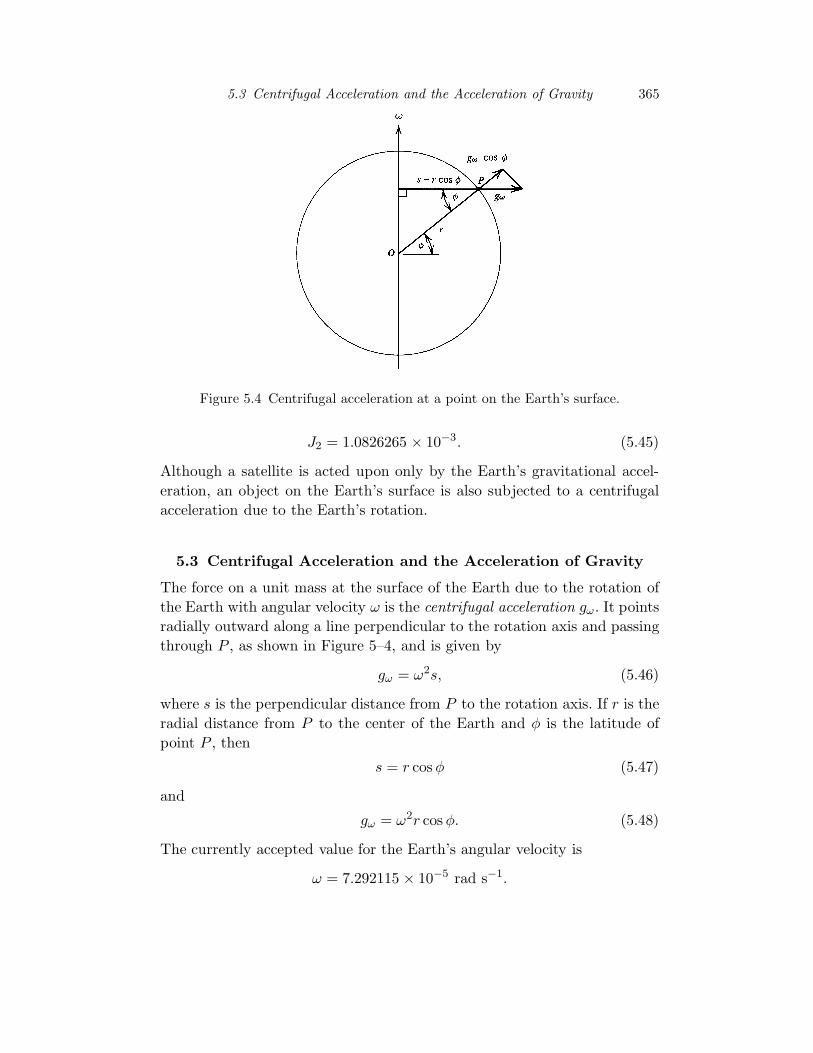
Figure 5.4 Centrifugal acceleration at a point on the Earth’s surface.

J2 = 1.0826265 × 10−3. (5.45)

Although a satellite is acted upon only by the Earth’s gravitational accel-eration, an object on the Earth’s surface is also subjected to a centrifugalacceleration due to the Earth’s rotation.

5.3 Centrifugal Acceleration and the Acceleration of Gravity

The force on a unit mass at the surface of the Earth due to the rotation ofthe Earth with angular velocity ω is the centrifugal acceleration gω. It pointsradially outward along a line perpendicular to the rotation axis and passingthrough P , as shown in Figure 5–4, and is given by

gω = ω2s, (5.46)

where s is the perpendicular distance from P to the rotation axis. If r is theradial distance from P to the center of the Earth and φ is the latitude ofpoint P , then

s = r cos φ (5.47)

and

gω = ω2r cos φ. (5.48)

The currently accepted value for the Earth’s angular velocity is

ω = 7.292115 × 10−5 rad s−1.

366 Gravity

Problem 5.2 Determine the ratio of the centrifugal acceleration to thegravitational acceleration at the Earth’s equator.

The gravitational and centrifugal accelerations of a mass at the Earth’ssurface combine to yield the acceleration of gravity g. Because gω ≪ gm, itis appropriate to add the radial component of the centrifugal accelerationto gm to obtain g; see Equations (5–16) and (5–17). As shown in Figure 5–4, the radial component of centrifugal acceleration points radially outward.In agreement with our sign convention that inward radial accelerations arepositive, the radial component of the centrifugal acceleration is

g′r = −gω cos φ = −ω2r cos2 φ. (5.49)

Therefore, the acceleration of gravity g is the sum of gm in Equation (5–44)and g′r:

g =GM

r2−

3GMa2J2

2r4(3 sin2 φ− 1) − ω2r cos2 φ.

(5.50)

Equation (5–50) gives the radially inward acceleration of gravity for a pointlocated on the surface of the model Earth at latitude φ and distance r fromthe center of mass.

5.4 The Gravitational Potential and the Geoid

By virtue of its position in a gravitational field, a mass m′ has gravitationalpotential energy. The energy can be regarded as the negative of the workdone on m′ by the gravitational force of attraction in bringing m′ from infin-ity to its position in the field. The gravitational potential V is the potentialenergy of m′ divided by its mass. Because the gravitational field is conser-vative, the potential energy per unit mass V depends only on the positionin the field and not on the path through which a mass is brought to thelocation. To calculate V for the rotationally distorted model Earth, we canimagine bringing a unit mass from infinity to a distance r from the centerof the model along a radial path. The negative of the work done on the unitmass by the gravitational field of the model is the integral of the productof the force per unit mass gm in Equation (5–44) with the increment of dis-tance dr (the acceleration of gravity and the increment dr are oppositelydirected):

V =! r

∞

"

GM

r′2−

3GMa2J2

2r′4(3 sin2 φ− 1)

#

dr′

5.4 The Gravitational Potential and the Geoid 367

(5.51)

or

V = −GM

r+

GMa2J2

2r3(3 sin2 φ− 1). (5.52)

In evaluating V , we assume that the potential energy at an infinite distancefrom the Earth is zero. The gravitational potential adjacent to the Earth isnegative; Earth acts as a potential well. The first term in Equation (5–52)is the gravitational potential of a point mass. It is also the gravitationalpotential outside any spherically symmetric mass distribution. The secondterm is the effect on the potential of the Earth model’s rotationally inducedoblateness. A gravitational equipotential surface is a surface on which V is aconstant. Gravitational equipotentials are spheres for spherically symmetricmass distributions.

Problem 5.3 (a) What is the gravitational potential energy of a 1-kg massat the Earth’s equator? (b) If this mass fell toward the Earth from a largedistance where it had zero relative velocity, what would be the velocity atthe Earth’s surface? (c) If the available potential energy was converted intoheat that uniformly heated the mass, what would be the temperature of themass if its initial temperature T0 = 100 K, c = 1 kJ kg−1 K−1, Tm = 1500K, and L = 400 kJ kg−1?

A comparison of Equations (5–44) and (5–52) shows that V is the integralof the radial component of the gravitational acceleration gm with respect tor. To obtain a gravity potential U which accounts for both gravitation andthe rotation of the model Earth, we can take the integral with respect to rof the radial component of the acceleration of gravity g in Equation (5–50)with the result that

U = −GM

r+

GMa2J2

2r3(3 sin2 φ− 1)

−1

2ω2r2 cos2 φ. (5.53)

A gravity equipotential is a surface on which U is a constant. Within a fewmeters the sea surface defines an equipotential surface. Therefore, elevationsabove or below sea level are distances above or below a reference equipoten-tial surface.

The reference equipotential surface that defines sea level is called the geoid.We will now obtain an expression for the geoid surface that is consistent withour second-order expansion of the gravity potential given in Equation (5–53). The value of the surface gravity potential at the equator is found by

368 Gravity

substituting r = a and φ = 0 in Equation (5–53) with the result

U0 = −GM

a

$

1 +1

2J2

%

−1

2a2ω2. (5.54)

The value of the surface gravity potential at the poles must also be U0

because we define the surface of the model Earth to be an equipotentialsurface. We substitute r = c (the Earth’s polar radius) and φ = ±π/2 intoEquation (5–53) and obtain

U0 = −GM

c

&

1 − J2

$

a

c

%2'

. (5.55)

The flattening (ellipticity) of this geoid is defined by

f ≡a − c

a. (5.56)

The flattening is very slight; that is, f ≪ 1. In order to relate the flatteningf to J2, we set Equations (5–54) and (5–55) equal and obtain

1 +1

2J2 +

1

2

a3ω2

GM=

a

c

&

1 − J2

$

a

c

%2'

. (5.57)

Substituting c = a(1 − f) and the neglecting quadratic and higher orderterms in f and J2, because f ≪ 1 and J2 ≪ 1, we find that

f =3

2J2 +

1

2

a3ω2

GM. (5.58)

Taking a3ω2/GM = 3.46139 × 10−3 and J2 = 1.0826265 × 10−3 from Equa-tion (5–45), we find from Equation (5–58) that f = 3.3546×10−3 . Retentionof higher order terms in the theory gives the more accurate value

f = 3.35281068 × 10−3 =1

298.257222. (5.59)

It should be emphasized that Equation (5–58) is valid only if the surface ofthe planetary body is an equipotential.

The shape of the model geoid is nearly that of a spherical surface; that is,if r0 is the distance to the geoid,

r0 ≈ a(1 − ε), (5.60)

where ε≪ 1. By setting U = U0 and r = r0 in Equation (5–53), substitutingEquation (5–54) for U0 and Equation (5–60) for r0, and neglecting quadraticand higher order terms in f , J2, a3ω2/GM , and ε, we obtain

ε =$

3

2J2 +

1

2

a3ω2

GM

%

sin2 φ. (5.61)

5.4 The Gravitational Potential and the Geoid 369

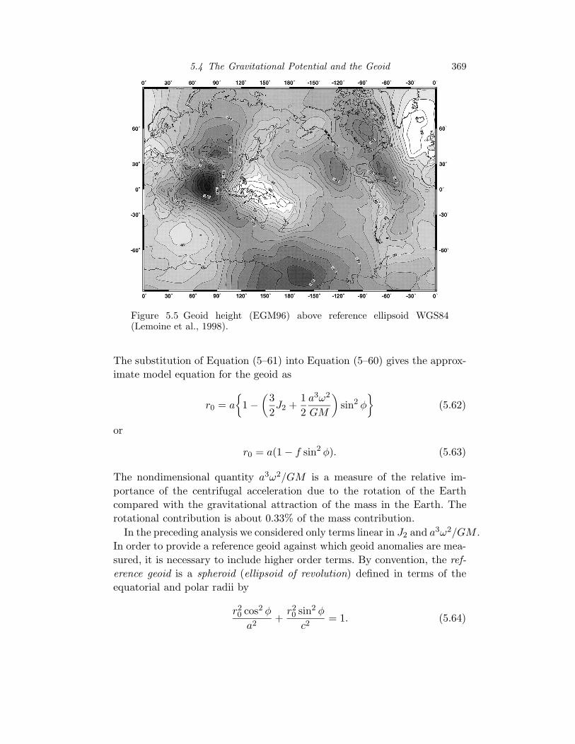
Figure 5.5 Geoid height (EGM96) above reference ellipsoid WGS84(Lemoine et al., 1998).

The substitution of Equation (5–61) into Equation (5–60) gives the approx-imate model equation for the geoid as

r0 = a"

1 −$

3

2J2 +

1

2

a3ω2

GM

%

sin2 φ#

(5.62)

or

r0 = a(1 − f sin2 φ). (5.63)

The nondimensional quantity a3ω2/GM is a measure of the relative im-portance of the centrifugal acceleration due to the rotation of the Earthcompared with the gravitational attraction of the mass in the Earth. Therotational contribution is about 0.33% of the mass contribution.

In the preceding analysis we considered only terms linear in J2 and a3ω2/GM .In order to provide a reference geoid against which geoid anomalies are mea-sured, it is necessary to include higher order terms. By convention, the ref-erence geoid is a spheroid (ellipsoid of revolution) defined in terms of theequatorial and polar radii by

r20 cos2 φ

a2+

r20 sin2 φ

c2= 1. (5.64)

370 Gravity

The eccentricity e of the spheroid is given by

e ≡$

a2 − c2

a2

%1/2

= (2f − f2)1/2. (5.65)

It is the usual practice to express the reference geoid in terms of the equa-torial radius and the flattening with the result

r20 cos2 φ

a2+

r20 sin2 φ

a2(1 − f)2= 1 (5.66)

or

r0 = a&

1 +(2f − f2)

(1 − f)2sin2 φ

'−1/2

. (5.67)

If Equation (5–67) is expanded in powers of f and if terms of quadraticand higher order in f are neglected, the result agrees with Equation (5–63).Equation (5–67) with a = 6378.137 km and f = 1/298.257222 defines thereference geoid.

The difference in elevation between the measured geoid and the referencegeoid ∆N is referred to as a geoid anomaly. A map of geoid anomalies isgiven in Figure 5–5. The maximum geoid anomalies are around 100 m; thisis about 0.5% of the 21-km difference between the equatorial and polar radii.Clearly, the measured geoid is very close to having the spheroidal shape ofthe reference geoid.

The major geoid anomalies shown in Figure 5–5 can be attributed to den-sity inhomogeneities in the Earth. A comparison with the distribution ofsurface plates given in Figure 1–1 shows that some of the major anomaliescan be directly associated with plate tectonic phenomena. Examples are thegeoid highs over New Guinea and Chile–Peru; these are clearly associatedwith subduction. The excess mass of the dense subducted lithosphere causesan elevation of the geoid. The negative geoid anomaly over China may beassociated with the continental collision between the Indian and Eurasianplates and the geoid low over the Hudson Bay in Canada may be associatedwith postglacial rebound (see Section 6–10). The largest geoid anomaly isthe negative geoid anomaly off the southern tip of India, which has an am-plitude of 100 m. No satisfactory explanation has been given for this geoidanomaly, which has no surface expression. A similar unexplained negativegeoid anomaly lies off the west coast of North America.

The definition of geoid anomalies relative to the reference geoid is some-what arbitrary. The reference geoid itself includes an averaging over den-sity anomalies within the Earth. An alternative approach is to define geoidanomalies relative to a hydrostatic geoid. The Earth is assumed to have a

5.4 The Gravitational Potential and the Geoid 371

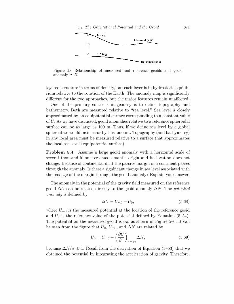
Figure 5.6 Relationship of measured and reference geoids and geoidanomaly ∆ N.

layered structure in terms of density, but each layer is in hydrostatic equilib-rium relative to the rotation of the Earth. The anomaly map is significantlydifferent for the two approaches, but the major features remain unaffected.

One of the primary concerns in geodesy is to define topography andbathymetry. Both are measured relative to “sea level.” Sea level is closelyapproximated by an equipotential surface corresponding to a constant valueof U . As we have discussed, geoid anomalies relative to a reference spheroidalsurface can be as large as 100 m. Thus, if we define sea level by a globalspheroid we would be in error by this amount. Topography (and bathymetry)in any local area must be measured relative to a surface that approximatesthe local sea level (equipotential surface).

Problem 5.4 Assume a large geoid anomaly with a horizontal scale ofseveral thousand kilometers has a mantle origin and its location does notchange. Because of continental drift the passive margin of a continent passesthrough the anomaly. Is there a significant change in sea level associated withthe passage of the margin through the geoid anomaly? Explain your answer.

The anomaly in the potential of the gravity field measured on the referencegeoid ∆U can be related directly to the geoid anomaly ∆N . The potentialanomaly is defined by

∆U = Um0 − U0, (5.68)

where Um0 is the measured potential at the location of the reference geoidand U0 is the reference value of the potential defined by Equation (5–54).The potential on the measured geoid is U0, as shown in Figure 5–6. It canbe seen from the figure that U0, Um0, and ∆N are related by

U0 = Um0 +$

∂U

∂r

%

r = r0

∆N, (5.69)

because ∆N/a ≪ 1. Recall from the derivation of Equation (5–53) that weobtained the potential by integrating the acceleration of gravity. Therefore,

372 Gravity

the radial derivative of the potential in Equation (5–69) is the accelerationof gravity on the reference geoid. To the required accuracy we can write

$

∂U

∂r

%

r = r0

= g0, (5.70)

where g0 is the reference acceleration of gravity on the reference geoid. Justas the measured potential on the reference geoid differs from U0, the mea-sured acceleration of gravity on the reference geoid differs from g0. However,for our purposes we can use g0 in Equation (5–69) for (∂U/∂r)r = r0 becausethis term is multiplied by a small quantity ∆N . Substitution of Equations(5–69) and (5–70) into Equation (5–68) gives

∆U = −g0∆N. (5.71)

A local mass excess produces an outward warp of gravity equipotentials andtherefore a positive ∆N and a negative ∆U . Note that the measured geoidessentially defines sea level. Deviations of sea level from the equipotentialsurface are due to lunar and solar tides, winds, and ocean currents. Theseeffects are generally a few meters.

The reference acceleration of gravity on the reference geoid is found bysubstituting the expression for r0 given by Equation (5–62) into Equation(5–50) and simplifying the result by neglecting quadratic and higher orderterms in J2 and a3ω2/GM . One finds

g0 =GM

a2

$

1+3

2J2 cos2 φ

%

+aω2(sin2 φ− cos2 φ).

(5.72)

To provide a standard reference acceleration of gravity against which gravityanomalies are measured, we must retain higher order terms in the equationfor g0. Gravity anomalies are the differences between measured values of g onthe reference geoid and g0. By international agreement in 1980 the referencegravity field was defined to be

g0 = 9.7803267715(1 + 0.0052790414 sin2 φ

+ 0.0000232718 sin4 φ

+ 0.0000001262 sin6 φ

+ 0.0000000007 sin8 φ), (5.73)

with g0 in m s−2. This is known as the 1980 Geodetic Reference System(GRS) (80) Formula. The standard reference gravity field given by Equation(5–73) is of higher order in φ than is the consistent quadratic approximation

5.5 Moments of Inertia 373

used to specify both g0 in Equation (5–72) and r0 in Equation (5–67). Thesuitable SI unit for gravity anomalies is mm s−2.

Problem 5.5 Determine the values of the acceleration of gravity at theequator and the poles using GRS 80 and the quadratic approximation givenin Equation (5–72).

Problem 5.6 By neglecting quadratic and higher order terms, show thatthe gravity field on the reference geoid can be expressed in terms of thegravity field at the equator ge according to

g0 = ge

&

1 +$

2ω2a3

GM−

3

2J2

%

sin2 φ'

. (5.74)

Problem 5.7 What is the value of the acceleration of gravity at a distanceb above the geoid at the equator (b ≪ a)?

5.5 Moments of Inertia

MacCullagh’s formula given in Equation (5–42) relates the gravitationalacceleration of an oblate planetary body to its principal moments of inertia.Thus, we can use the formula, together with measurements of a planet’sgravitational field by flyby or orbiting spacecraft, for example, to constrainthe moments of inertia of a planet. Since the moments of inertia reflecta planet’s overall shape and internal density distribution, we can use thevalues of the moments to learn about a planet’s internal structure. For thispurpose it is helpful to have expressions for the moments of inertia of somesimple bodies such as spheres and spheroids.

The principal moments of inertia of a spherically symmetric body are allequal, A = B = C, because the mass distribution is the same about any axispassing through the center of the body. For simplicity, we will determine themoment of inertia about the polar axis defined by θ = 0. For a sphericalbody of radius a, substitution of Equations (5–6) and (5–7) into Equation(5–26) gives

C =! 2π

0

! π

0

! a

0ρ(r′)r′4 sin3 θ′ dr′ dθ′ dψ′. (5.75)

Integration over the angles ψ′ and θ′ results in! 2π

0dψ′ = 2π

and! π

0sin3 θ′ dθ′ =

&

1

3cos3 θ′ − cos θ′

'π

0=

4

3,

374 Gravity

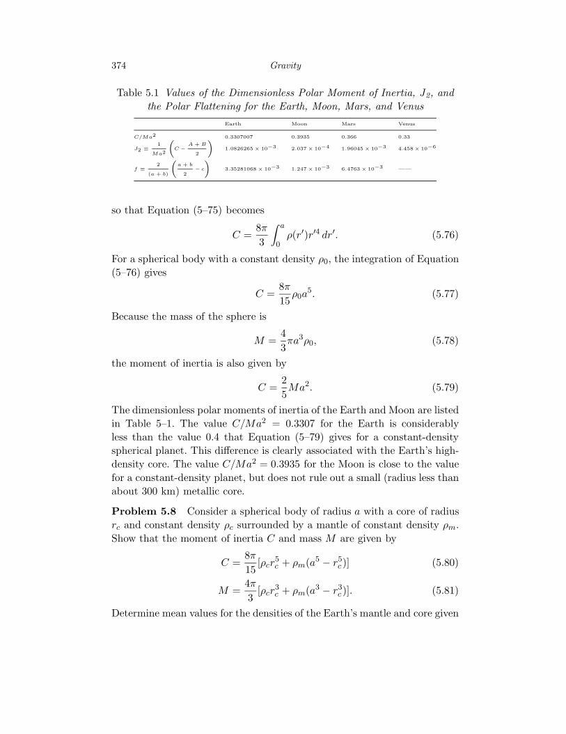
Table 5.1 Values of the Dimensionless Polar Moment of Inertia, J2, andthe Polar Flattening for the Earth, Moon, Mars, and Venus

Earth Moon Mars Venus

C/Ma2 0.3307007 0.3935 0.366 0.33

J2 ≡

1

Ma2

(

C −

A + B

2

)

1.0826265 × 10−3 2.037 × 10−4 1.96045 × 10−3 4.458 × 10−6

f ≡

2

(a + b)

(

a + b

2− c

)

3.35281068 × 10−3 1.247 × 10−3 6.4763 × 10−3 ——

so that Equation (5–75) becomes

C =8π

3

! a

0ρ(r′)r′4 dr′. (5.76)

For a spherical body with a constant density ρ0, the integration of Equation(5–76) gives

C =8π

15ρ0a

5. (5.77)

Because the mass of the sphere is

M =4

3πa3ρ0, (5.78)

the moment of inertia is also given by

C =2

5Ma2. (5.79)

The dimensionless polar moments of inertia of the Earth and Moon are listedin Table 5–1. The value C/Ma2 = 0.3307 for the Earth is considerablyless than the value 0.4 that Equation (5–79) gives for a constant-densityspherical planet. This difference is clearly associated with the Earth’s high-density core. The value C/Ma2 = 0.3935 for the Moon is close to the valuefor a constant-density planet, but does not rule out a small (radius less thanabout 300 km) metallic core.

Problem 5.8 Consider a spherical body of radius a with a core of radiusrc and constant density ρc surrounded by a mantle of constant density ρm.Show that the moment of inertia C and mass M are given by

C =8π

15[ρcr

5c + ρm(a5 − r5

c )] (5.80)

M =4π

3[ρcr

3c + ρm(a3 − r3

c )]. (5.81)

Determine mean values for the densities of the Earth’s mantle and core given

5.5 Moments of Inertia 375

C = 8.04 × 1037 kg m2, M = 5.97 × 1024 kg, a = 6378 km, and rc = 3486km.

We will next determine the principal moments of inertia of a constant-density spheroid defined by

r0 =ac

(a2 cos2 θ + c2 sin2 θ)1/2. (5.82)

This is a rearrangement of Equation (5–64) with the colatitude θ being usedin place of the latitude φ. By substituting Equations (5–6) and (5–7) intoEquations (5–26) and (5–29), we can write the polar and equatorial momentsof inertia as

C = ρ! 2π

0

! r0

0

! π

0r′4 sin3 θ′ dθ′ dr′ dψ′ (5.83)

A = ρ! 2π

0

! r0

0

! π

0r′4 sin θ′

× (sin2 θ′ sin2 ψ′ + cos2 θ′) dθ′ dr′ dψ′, (5.84)

where the upper limit on the integral over r′ is given by Equation (5–82)and B = A for this axisymmetric body. The integrations over ψ′ and r′ arestraightforward and yield

C =2

5πρa5c5

! π

0

sin3 θ′ dθ′

(a2 cos2 θ′ + c2 sin2 θ′)5/2(5.85)

A =1

2C +

2

5πρa5c5

! π

0

cos2 θ′ sin θ′ dθ′

(a2 cos2 θ′ + c2 sin2 θ′)5/2.

(5.86)

The integrals over θ′ can be simplified by introducing the variable x =cos θ′(dx = − sin θ′ dθ′, sin θ′ = (1 − x2)1/2) with the result

C =2

5πρa5c5

! 1

−1

(1 − x2) dx

[c2 + (a2 − c2)x2]5/2(5.87)

A =1

2C +

2

5πρa5c5

! 1

−1

x2 dx

[c2 + (a2 − c2)x2]5/2.

(5.88)

From a comprehensive tabulation of integrals we find

! 1

−1

dx

{c2 + (a2 − c2)x2}5/2=

2

3

(2a2 + c2)

c4a3(5.89)

376 Gravity

! 1

−1

x2 dx

{c2 + (a2 − c2)x2}5/2=

2

3

1

c2a3. (5.90)

By substituting Equations (5–89) and (5–90) into Equations (5–87) and (5–88), we obtain

C =8

15πρa4c (5.91)

A =4

15πρa2c(a2 + c2). (5.92)

These expressions for the moments of inertia can be used to determine J2

for the spheroid. The substitution of Equations (5–91) and (5–92) into thedefinition of J2 given in Equation (5–43), together with the equation for themass of a constant-density spheroid

M =4π

3ρa2c, (5.93)

yields

J2 =1

5

$

1 −c2

a2

%

. (5.94)

Consistent with our previous assumption that J2 ≪ 1 and (1 − c/a) ≪ 1this reduces to

J2 =2

5

$

1 −c

a

%

=2f

5. (5.95)

Equation (5–95) relates J2 to the flattening of a constant-density planetarybody. The deviation of the near-surface layer from a spherical shape pro-duces the difference in polar and equatorial moments of inertia in such abody. For a planet that does not have a constant density, the deviation fromspherical symmetry of the density distribution at depth also contributes tothe difference in moments of inertia.

If the planetary surface is also an equipotential surface, Equation (5–58)is valid. Substitution of Equation (5–95) into that relation gives

f =5

4

a3ω2

GM(5.96)

or

J2 =1

2

a3ω2

GM. (5.97)

These are the values of the flattening and J2 expected for a constant-density,rotating planetary body whose surface is a gravity equipotential.

Observed values of J2 and f are given in Table 5–1. For the Earth J2/f =

5.5 Moments of Inertia 377

0.3229 compared with the value 0.4 given by Equation (5–95) for a constant-density body. The difference can be attributed to the variation of densitywith depth in the Earth and the deviations of the density distribution atdepth from spherical symmetry.

For the Moon, where a constant-density theory would be expected tobe valid, J2/f = 0.16. However, both J2 and f are quite small. The ob-served difference in mean equatorial and polar radii is (a + b)/2 − c = 2km, which is small compared with variations in lunar topography. Thereforethe observed flattening may be influenced by variations in crustal thick-ness. Because the Moon is tidally coupled to theEarth so that the same side ofthe Moon always faces the Earth, the rotation of the Moon is too small toexplain the observed value of J2. However, the present flattening may bea relic of a time when the Moon was rotating more rapidly. At that timethe lunar lithosphere may have thickened enough so that the strength of theelastic lithosphere was sufficient to preserve the rotational flattening.

For Mars, a3ω2/GM = 4.59×10−3 and J2 = 1.960×10−3. From Equation(5–58) the predicted value for the dynamic flattening is 5.235 × 10−3. Thiscompares with the observed flattening of 6.4763×10−3 . Again the differencemay be attributed to the preservation of a fossil flattening associated witha higher rotational velocity in the past. The ratio of J2 to the observedflattening is 0.3027; this again is considerably less than the value of 0.4 fora constant-density planet from Equation (5–95).

Problem 5.9 Assuming that the difference in moments of inertia C −Ais associated with a nearsurface density ρm and the mass M is associatedwith a mean planetary density ρ̄, show that

J2 =2

5

ρm

ρ̄f. (5.98)

Determine the value of ρm for the Earth by using the measured values ofJ2, ρ̄, and f . Discuss the value obtained.

Problem 5.10 Assume that the constant-density theory for the momentsof inertia of a planetary body is applicable to the Moon. Determine therotational period of the Moon that gives the measured value of J2.

Problem 5.11 Take the observed values of the flattening and J2 for Marsand determine the corresponding period of rotation. How does this comparewith the present period of rotation?

378 Gravity

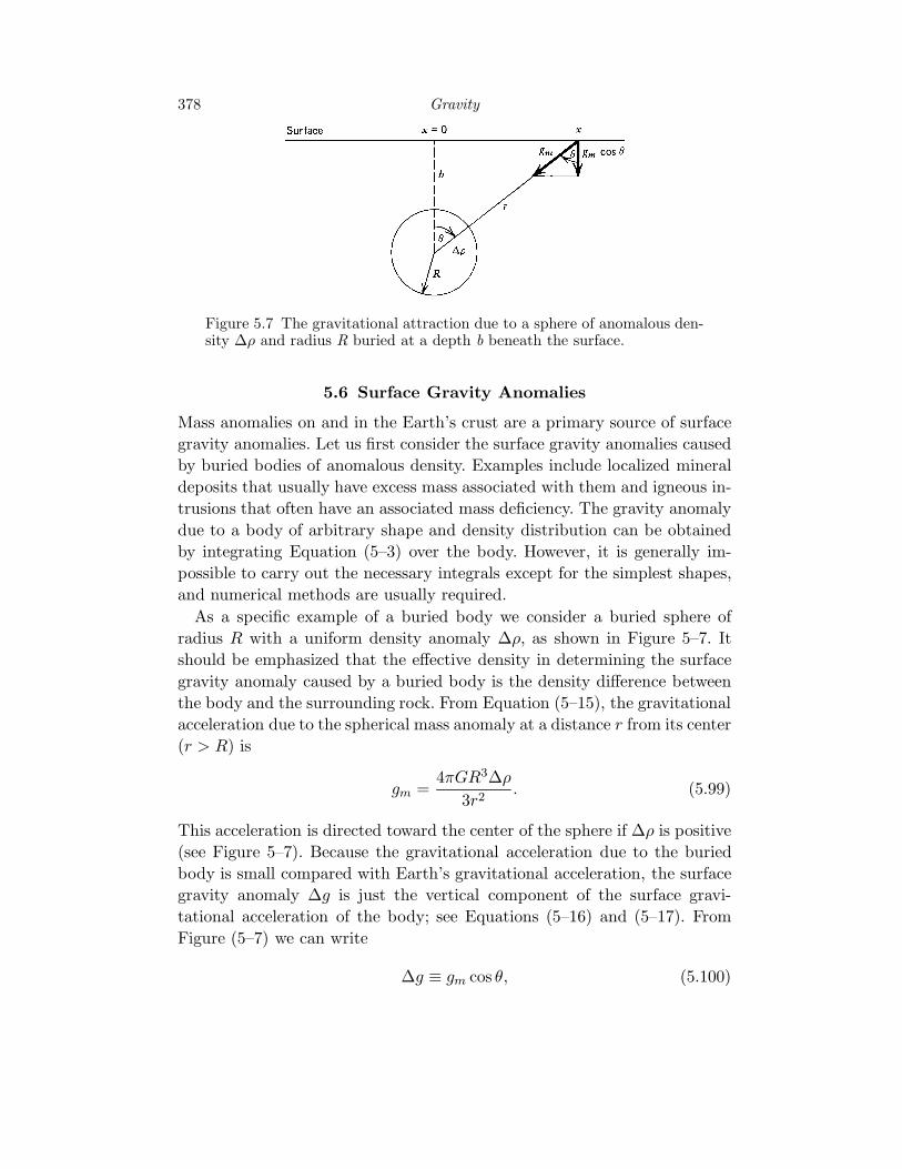
Figure 5.7 The gravitational attraction due to a sphere of anomalous den-sity ∆ρ and radius R buried at a depth b beneath the surface.

5.6 Surface Gravity Anomalies

Mass anomalies on and in the Earth’s crust are a primary source of surfacegravity anomalies. Let us first consider the surface gravity anomalies causedby buried bodies of anomalous density. Examples include localized mineraldeposits that usually have excess mass associated with them and igneous in-trusions that often have an associated mass deficiency. The gravity anomalydue to a body of arbitrary shape and density distribution can be obtainedby integrating Equation (5–3) over the body. However, it is generally im-possible to carry out the necessary integrals except for the simplest shapes,and numerical methods are usually required.

As a specific example of a buried body we consider a buried sphere ofradius R with a uniform density anomaly ∆ρ, as shown in Figure 5–7. Itshould be emphasized that the effective density in determining the surfacegravity anomaly caused by a buried body is the density difference betweenthe body and the surrounding rock. From Equation (5–15), the gravitationalacceleration due to the spherical mass anomaly at a distance r from its center(r > R) is

gm =4πGR3∆ρ

3r2. (5.99)

This acceleration is directed toward the center of the sphere if ∆ρ is positive(see Figure 5–7). Because the gravitational acceleration due to the buriedbody is small compared with Earth’s gravitational acceleration, the surfacegravity anomaly ∆g is just the vertical component of the surface gravi-tational acceleration of the body; see Equations (5–16) and (5–17). FromFigure (5–7) we can write

∆g ≡ gm cos θ, (5.100)

5.6 Surface Gravity Anomalies 379

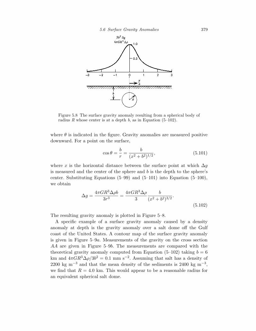
Figure 5.8 The surface gravity anomaly resulting from a spherical body ofradius R whose center is at a depth b, as in Equation (5–102).

where θ is indicated in the figure. Gravity anomalies are measured positivedownward. For a point on the surface,

cos θ =b

r=

b

(x2 + b2)1/2, (5.101)

where x is the horizontal distance between the surface point at which ∆gis measured and the center of the sphere and b is the depth to the sphere’scenter. Substituting Equations (5–99) and (5–101) into Equation (5–100),we obtain

∆g =4πGR3∆ρb

3r3=

4πGR3∆ρ

3

b

(x2 + b2)3/2.

(5.102)

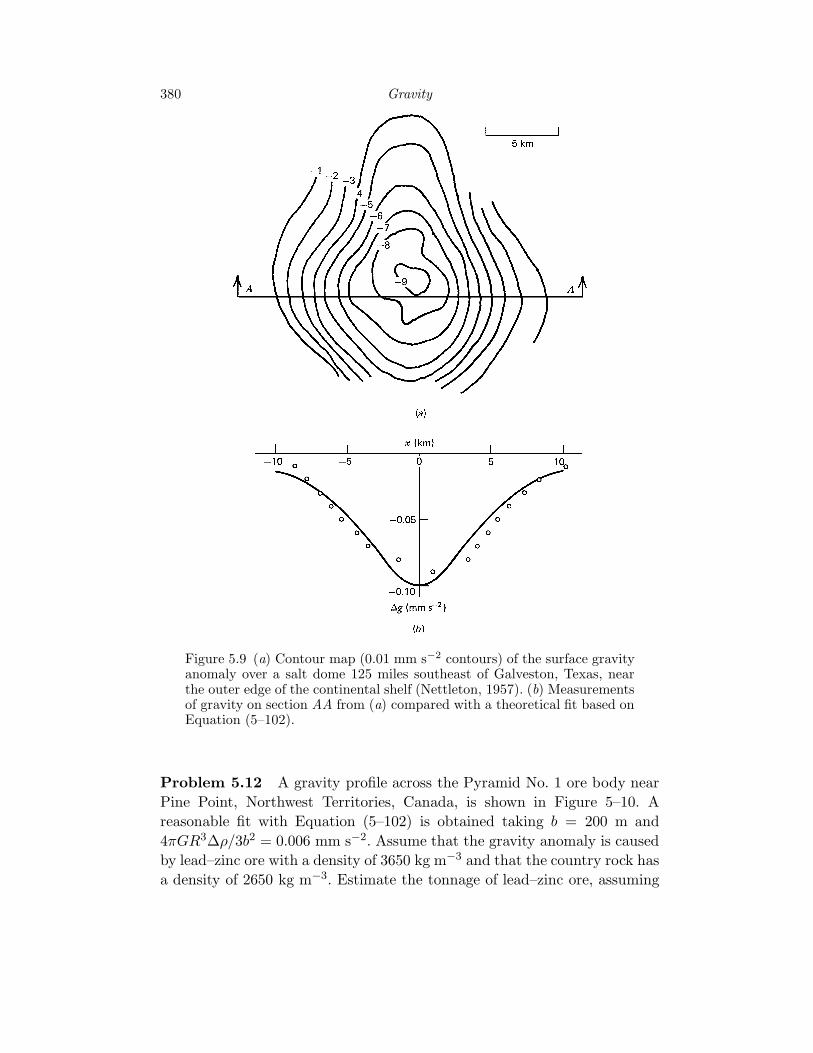
The resulting gravity anomaly is plotted in Figure 5–8.A specific example of a surface gravity anomaly caused by a density

anomaly at depth is the gravity anomaly over a salt dome off the Gulfcoast of the United States. A contour map of the surface gravity anomalyis given in Figure 5–9a. Measurements of the gravity on the cross sectionAA are given in Figure 5–9b. The measurements are compared with thetheoretical gravity anomaly computed from Equation (5–102) taking b = 6km and 4πGR3∆ρ/3b2 = 0.1 mm s−2. Assuming that salt has a density of2200 kg m−3 and that the mean density of the sediments is 2400 kg m−3,we find that R = 4.0 km. This would appear to be a reasonable radius foran equivalent spherical salt dome.

380 Gravity

Figure 5.9 (a) Contour map (0.01 mm s−2 contours) of the surface gravityanomaly over a salt dome 125 miles southeast of Galveston, Texas, nearthe outer edge of the continental shelf (Nettleton, 1957). (b) Measurementsof gravity on section AA from (a) compared with a theoretical fit based onEquation (5–102).

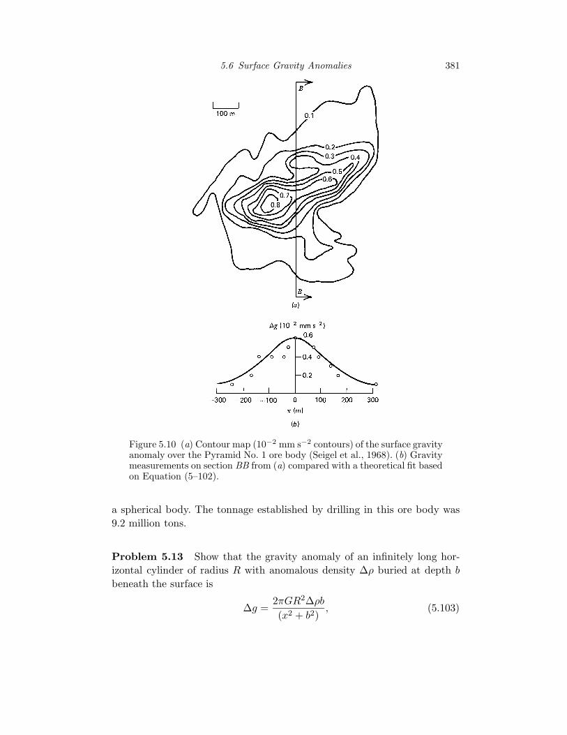
Problem 5.12 A gravity profile across the Pyramid No. 1 ore body nearPine Point, Northwest Territories, Canada, is shown in Figure 5–10. Areasonable fit with Equation (5–102) is obtained taking b = 200 m and4πGR3∆ρ/3b2 = 0.006 mm s−2. Assume that the gravity anomaly is causedby lead–zinc ore with a density of 3650 kg m−3 and that the country rock hasa density of 2650 kg m−3. Estimate the tonnage of lead–zinc ore, assuming

5.6 Surface Gravity Anomalies 381

Figure 5.10 (a) Contour map (10−2 mm s−2 contours) of the surface gravityanomaly over the Pyramid No. 1 ore body (Seigel et al., 1968). (b) Gravitymeasurements on section BB from (a) compared with a theoretical fit basedon Equation (5–102).

a spherical body. The tonnage established by drilling in this ore body was9.2 million tons.

Problem 5.13 Show that the gravity anomaly of an infinitely long hor-izontal cylinder of radius R with anomalous density ∆ρ buried at depth bbeneath the surface is

∆g =2πGR2∆ρb

(x2 + b2), (5.103)

382 Gravity

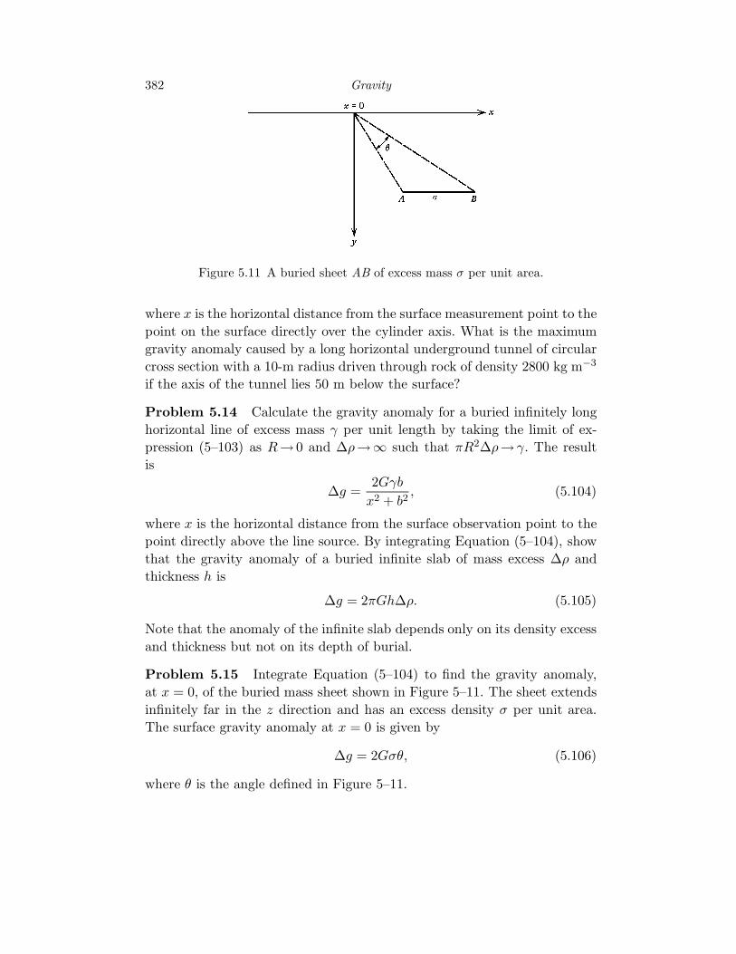
Figure 5.11 A buried sheet AB of excess mass σ per unit area.

where x is the horizontal distance from the surface measurement point to thepoint on the surface directly over the cylinder axis. What is the maximumgravity anomaly caused by a long horizontal underground tunnel of circularcross section with a 10-m radius driven through rock of density 2800 kg m−3

if the axis of the tunnel lies 50 m below the surface?

Problem 5.14 Calculate the gravity anomaly for a buried infinitely longhorizontal line of excess mass γ per unit length by taking the limit of ex-pression (5–103) as R→ 0 and ∆ρ→∞ such that πR2∆ρ→ γ. The resultis

∆g =2Gγb

x2 + b2, (5.104)

where x is the horizontal distance from the surface observation point to thepoint directly above the line source. By integrating Equation (5–104), showthat the gravity anomaly of a buried infinite slab of mass excess ∆ρ andthickness h is

∆g = 2πGh∆ρ. (5.105)

Note that the anomaly of the infinite slab depends only on its density excessand thickness but not on its depth of burial.

Problem 5.15 Integrate Equation (5–104) to find the gravity anomaly,at x = 0, of the buried mass sheet shown in Figure 5–11. The sheet extendsinfinitely far in the z direction and has an excess density σ per unit area.The surface gravity anomaly at x = 0 is given by

∆g = 2Gσθ, (5.106)

where θ is the angle defined in Figure 5–11.