GENETICS OF COTTON FIBER ELONGATION

A Dissertation

by

ENG HWA NG

Submitted to the Office of Graduate Studies of

Texas A&M University

in partial fulfillment of the requirements for the degree of

DOCTOR OF PHILOSOPHY

Chair of Committee, C. Wayne Smith

Committee Members, Eric Hequet

Steven Hague

J. Tom Cothren

Yog Raj

Head of Department, David Baltensperger

August 2013

Major Subject: Plant Breeding

Copyright 2013 Eng Hwa Ng

ii

ABSTRACT

Fiber elongation (ability to stretch before breaking) is one of the key components

in determining overall yarn quality. Elongation in U.S. upland cotton (G. hirsutum L.)

has remained largely neglected due to: absence of monetary incentives for growers to

produce high elongation cotton; lack of research interests among breeders; and absence

of a reliable fiber testing system for elongation. This study was conducted to determine

the genetics of cotton fiber elongation via a diallel and generation means analysis

(GMA). Findings from this study should lay the foundation for future breeding work in

cotton fiber elongation.

Of the seven distinctive upland parents used for the diallel study, general

combining ability was far more prominent than specific combing ability for fiber

elongation. Cultivar PSC 355 and Dever experimental line were the two parents

identified as good combiners for fiber elongation in this study. The slight negative

correlation between fiber elongation and strength remained true. Highly significant

negative correlation was observed between fiber upper half mean length and elongation.

Both Stelometer and HVI elongation measurements correlated well with values of 0.85

and 0.82 in 2010 and 2011, respectively. For the six families used in the GMA analysis,

additive genetic control was prevalent over dominance effect. Based on the scaling test,

no significant epistatic interaction was detected for fiber elongation. As expected,

additive variance constituted a much larger portion of total genetic variation in fiber

elongation than the dominance variance. On average, larger numbers of effective factor

iii

were identified in fiber elongation than all other fiber traits tested, suggesting that

parents used in the GMA study are carrying different genetic materials/ loci for fiber

elongation. Considerable gains in fiber elongation may be achieved by selectively

crossing these materials in a pure-line breeding scheme while holding other important

fiber traits constant.

iv

ACKNOWLEDGEMENTS

I would like to thank my committee chair, Dr. C.W. Smith, and my committee

members, Dr. Eric Hequet, Dr. Steve Hague, Dr. Tom Cothren and Dr. Yog Raj (special

appointment member) for their support and guidance throughout the course of this

research.

I would like to also thank Cotton Improvement Lab, technician Mrs. D. Deno,

fellow graduate students and student workers at the lab for their help in managing my

field plots in College Station. Thanks to the Fiber and Biopolymer Research institute,

Lubbock for providing the fiber testing instrument and allowing me to perform my fiber

analysis. I also want to extent my gratitude to Monsanto Fellowship in breeding, Texas

A&M AgriLife Research, and Cotton Inc. for funding my Ph.D. research at Texas A&M

University.

Finally, thanks to my parents and friends for their patience and encouragements

for the past few years.

v

NOMENCLATURE

Elo-H Fiber elongation (HVI)

Elo-S Fiber elongation (Stelometer)

GCA General combining ability

GxE Genotype by environment interaction

HVI High volume instrument

Mic Micronaire (HVI)

SCA Specific combining ability

Str-H Fiber strength (HVI)

Str-S Fiber strength (Stelometer)

UHML Upper-half mean length (HVI)

UI Uniformity index

vi

TABLE OF CONTENTS

Page

ABSTRACT ................................................................................................................. ii

ACKNOWLEDGEMENTS ......................................................................................... iv

NOMENCLATURE ..................................................................................................... v

TABLE OF CONTENTS ............................................................................................. vi

LIST OF TABLES ....................................................................................................... viii

CHAPTER I INTRODUCTION .................................................................................. 1

CHAPTER II LITERATURE REVIEW ...................................................................... 7

Cotton, a fiber crop ........................................................................................... 7

Cotton fiber classing ......................................................................................... 8

Fiber elongation ................................................................................................ 9

HVI elongation ..................................................................................... 11

Stelometer elongation ........................................................................... 12

Qualitative versus quantitative traits ................................................................ 13

Variances .......................................................................................................... 14

Epistasis ............................................................................................................ 15

Environment ..................................................................................................... 17

Heritability ....................................................................................................... 18

Genetic gain ...................................................................................................... 19

Effective factors ............................................................................................... 20

Statistical design for crop improvement ........................................................... 22

Diallel analysis ..................................................................................... 22

Generation means analysis ................................................................... 24

CHAPTER III DIALLEL ANALYSIS FOR FIBER ELONGATION ........................ 27

Plant materials .................................................................................................. 27

Material and methods ....................................................................................... 27

Early screening and generation development ....................................... 27

Field study ............................................................................................ 30

Stelometer analysis ............................................................................... 31

HVI analysis ......................................................................................... 32

vii

Statistical analysis ............................................................................................ 32

Diallel analysis ..................................................................................... 33

Correlation analysis .............................................................................. 34

Results and discussion ...................................................................................... 35

HVI ....................................................................................................... 35

Stelometer ............................................................................................. 41

CHAPTER IV SUMMARY OF DIALLEL ANALYSIS ............................................ 48

CHAPTER V GENERATION MEANS ANALYSIS OF FIBER ELONGATION .... 51

Plant materials .................................................................................................. 51

Material and methods ....................................................................................... 51

Early screening and generation development ....................................... 51

Field study and fiber testing ................................................................. 53

Statistical analysis ............................................................................................ 54

Generation means analysis ................................................................... 54

Variance and heritability estimates ...................................................... 57

Gain from selection and effective factors ............................................ 58

Results and discussions .................................................................................... 60

CHAPTER VI SUMMARY OF GENERATION MEANS ANALYSIS .................... 88

CHAPTER VII CONCLUSIONS ................................................................................ 90

REFERENCES ............................................................................................................. 92

viii

LIST OF TABLES

TABLE Page

1 Pedigrees of parental genotypes for diallel analysis ....................................... 28

2 Elongation prescreening for seven parental genotypes using Stelometer....... 30

3 Mean squares of combined ANOVA of HVI fiber properties measured in

2010 and 2011 in College Station, TX ........................................................... 37

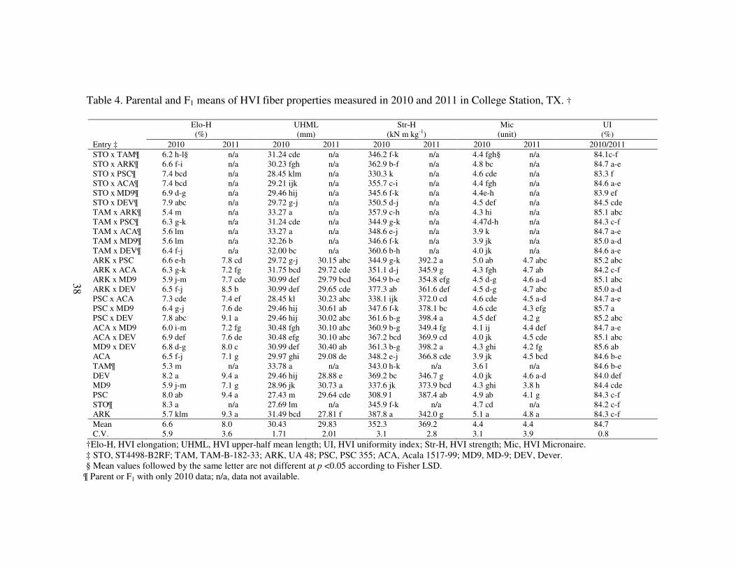
4 Parental and F1 means of HVI fiber properties measured in 2010 and 2011

in College Station, TX .................................................................................... 38

5 Mean squares of GCA and SCA for HVI fiber properties in 2010 and 2011

in College Station, TX .................................................................................... 39

6 GCA estimates for HVI fiber properties in 2010 and 2011 in College

Station, TX ...................................................................................................... 39

7 SCA estimates for HVI fiber properties in 2010 and 2011 in College

Station, TX ...................................................................................................... 40

8 Combined ANOVA of Stelometer fiber properties measured in 2010 and

2011 in College Station, TX ........................................................................... 41

9 Parental and F1 means of Stelometer fiber properties measured in 2010 and

2011 in College Station, TX ........................................................................... 42

10 Mean squares of GCA and SCA for Stelometer fiber properties in 2010

and 2011 in College Station, TX .................................................................... 44

11 GCA estimates for Stelometer fiber properties in 2010 and 2011 in College

Station, TX ...................................................................................................... 44

12 SCA estimates for Stelometer fiber properties in 2010 and 2011 in College

Station, TX ...................................................................................................... 45

13 Correlation analysis of fiber properties measured by Stelometer and HVI

in 2010 and 2011 in College Station, TX ....................................................... 47

14 Pedigrees of parental genotypes for GMA analysis........................................ 52

ix

15 Analysis of variance for HVI fiber properties for all GMA families in 2011

and 2012 in College Station, TX .................................................................... 61

16 Means of HVI fiber properties for six generations for GMA families in

2011 and 2012 in College Station, TX ........................................................... 64

17 Test for homogeneity of variance on all HVI fiber traits for all GMA

families in 2011 and 2012 in College Station, TX ......................................... 70

18 Hayman’s estimates for all HVI fiber traits in 2011 and 2012 in College

Station, TX ...................................................................................................... 72

19 Variance components and narrow sense (h2) heritability estimates for all

HVI fiber traits in 2011 and 2012 in College Station, TX .............................. 76

20 Effective gene estimates and gain from selection for all HVI fiber traits in

2011 and 2012 in College Station, TX ........................................................... 83

1

CHAPTER I

INTRODUCTION

Based on the recent National Cotton Council statistics, cotton (Gossypium spp.)

production covers roughly 13.6 million acres of farmland in the United States (U.S.)

with an estimated annual production of 15 million bales. It is currently projected that

12.9 million bales of cotton produced in the U.S. will be exported in 2012, which

accounts for more that 80% of total cotton produced in the U.S. (National Cotton

Council, 2012). Of all the cotton grown in the U.S., more than 95% of cultivars grown

are Upland type cotton (G. hirsutum L.) while Pima type (G. barbadense) accounts for

the remainder of total acreage. Texas is the largest producer of upland cotton with an

annual acreage of approximately five million acres (Cotton Incorporated, 2012). Due to

the increased exportation demands and quality expectations, it is important for U.S.

cotton to remain competitive not only in yield but also in fiber quality.

In recent years, modernization in yarn and textile industries has mandated that

U.S. cotton meet certain international quality criteria. For textile manufacturers, better

yarn production requires cotton fibers with improved spinning performance. Previous

spinning studies have shown that stronger yarns are often spun with fibers that are long,

strong and fine (Gregory et al., 2012; Joy et al. 2010). Currently, there are two

commonly used spinning systems worldwide. The rotor spinning system is a high speed

system that utilizes fibers with shorter staple length (about 25.4 mm) and good tenacity.

This type of system was used predominantly in the U.S. in the early 90s, and most of the

2

cotton produced domestically was specifically targeted for such a system. Ring spinning

is a slower spinning technique often used with higher quality fibers (longer staple length

and finer fibers) to produce finer and stronger yarns (Foulk, 2007). Recent shifts in

consumer preference for a better quality end product have caused many textile

manufacturers to adopt ring spinning technology to meet the demands. According to

statistics from the International Textile Manufacturers Federation (ITMF, 2012), there

were 110 million ring spinning spindle capacity installed in China as of 2009 as demand

for rotor spun yarn steadily declined over the years. With such a large capacity for ring

spun type yarn, it is inevitable that U.S. growers would want to produce higher quality

fibers for better global marketability and that breeders would want to develop better

cotton cultivars to meet the demand. Concomitantly, as textile manufacturers constantly

strive for higher output, cotton fibers are also subjected to harsher processing

environments. The only way to keep up with such high throughput is to have cotton with

improved tensile properties (strength and elongation).

For fiber quality measurement, the High Volume Instrument (HVI) (Uster,

2012a) has been the industry standard in the U.S. since the 1980s (Bradow and

Davidonis, 2000). HVI measures fiber strength (kN m kg-1

), upper half mean length

(mm), micronaire (units), color, elongation (%) and uniformity index (ratio) for every

cotton bale produced in the United States. Currently, pricing is based on a combination

of strength, length, uniformity index, micronaire, color and trash content as determined

by HVI, and premiums are given when cotton exceeds certain quality traits to promote

production of higher quality cotton (National Cotton Council, 2012). The monetary

3

incentive has been a huge driving force for breeders to improve certain fiber traits,

especially those thought to be associated with yarn quality such as length, strength and

uniformity index. However, these fiber data may not always be a good indicator for the

actual yarn performance. May and Jividen (1999) showed only moderate correlation

between various fiber traits and their corresponding yarn performance. To better

improve yarn quality, breeders always should consider the importance of every fiber

property prior to making selections. Crop improvement programs usually focus on traits

with high heritability that correlate positively with yield (Scholl and Miller, 1976).

Fiber elongation is valuable information that is often neglected by breeders and

the industry due to various reasons. HVI is a high speed and low cost method for

obtaining repeatable elongation. However, the lack of standardized calibration cotton

samples for HVI elongation renders elongation measurements unreliable from machine

to machine (Benzina et al., 2007), and there is no incentive to improve fiber elongation

in modern cotton cultivars because it is not part of the cotton pricing structure. The

effect of fiber elongation on yarn work-to-break has been inconclusive also. Studies by

Green and Culp (1990) indicated that fiber elongation is slightly negatively correlated

with yarn strength. Benzina et al. (2007) tested fiber bundle elongation with a modified

version of a tensile testing instrument (UT 350®

) (Tensometric Company Ltd.) and

proposed that fiber elongation is crucial in determining the overall work-to-break for

fiber bundles, which is a function of strength and elongation. Moreover, Benzina et al.

verified that the negative correlation for fiber bundle elongation and fiber strength was

4

weak and concluded that simultaneous improvement of fiber elongation and strength is

feasible.

Fibers with strength in the premium range, but with lower elongation, may

actually rupture more easily than fibers that have moderate strength but superior

elongation values. Cotton markets currently consider cotton with strength above 294.2

kN m kg-1

(30 g/tex) to be strong regardless of elongation, and this can be a false

classification of true fiber tensile properties. Instead, to truly measure fiber tensile

properties, work-to-break may be a superior measurement than relying on either strength

or elongation alone. According to Meredith (1945), if Hooke’s Law were to be obeyed,

work-to-break is the area under the stress-strain curve up to the maximum force. In the

sense of fiber and textile quality, the work-to-break reflects the total amount of energy

needed to rupture a bundle of fibers of a specified weight.

Stelometer (Uster, 2012b) is an improved version of the Pressley strength tester.

It is used to measure fiber bundle elongation and strength (the Pressley cannot measure

elongation). A constant rate of load is applied to break a fiber bundle, and cotton

standards for Stelometer are used to calibrate the instrument. It allows for accurate and

repeatable strength and elongation measurements. However, although more reliable,

Stelometer elongation is often not fully utilized due to the lower testing speed and the

limited amount of fiber properties obtainable compared to the current HVI system. A

good comparison between HVI and Stelometer measured elongation and strength from

multiple representative upland cotton cultivars would definitely be useful in gauging the

5

pros and cons of each instrument. The need to accurately and precisely measure

elongation may be growing with increasing interest in fiber elongation.

Genetic fixation may be defined as maintaining stable inheritance of favorable

alleles or traits over generations of selection. Additive genes with high heritability often

allow for rapid genetic fixation and gain. In upland cotton, genetic gain in fiber quality

traits such as fiber length and strength has been less than desired. Some studies even

suggested fiber strength to be negatively correlated with increased fiber yield (Miller and

Rawling, 1967; Scholl and Miller, 1976; Tang et al., 1996). Therefore, in order to truly

improve spinning performance and not sacrifice yield, it is important for breeders to

consider alternative fiber traits such as fiber elongation. A quantitative trait loci (QTL)

study on fiber elongation has shown that fiber elongation is a highly heritable trait with

minimal genotype by environment (GxE) effect even under stressful environments

(Paterson et al., 2003). In addition, genetic studies completed on various upland type

cotton cultivars have shown fiber elongation to have predominantly additive gene action,

more so than fiber strength in many cases (May and Taylor, 1998; Quisenberry, 1975).

There are various experimental designs a breeder could use to investigate genetic

components for traits of interest. Identifying a proper design could lead to optimized

genetic gain over the years with minimal resources (Fehr, 1991). High general

combining ability (GCA), indicating additive gene action and high narrow sense

heritability (h2), among a given set of parents is desirable. Assuming a relative high h

2

for elongation, as indicated by some studies, it would be interesting to further dissect the

genetic component governing elongation in several prominent upland cotton cultivars in

6

Texas. To do so, a diallel analysis without reciprocals (model 1, method 2) could be used

to partition the general combining ability (GCA) and specific combining ability (SCA)

for elongation (Griffing, 1956a; Griffing 1956b). In addition, generation means analysis

could be used to further investigate gene actions involved in elongation via multiple

generations generated from specific parental combinations. Objectives for this study are:

1. To determine elongation values for seven representative upland cotton genotypes

with Stelometer and HVI;

2. To conduct a diallel analysis with seven upland cotton genotypes to partition

GCA and SCA for fiber elongation using Stelometer and HVI;

3. To determine the correlation between Stelometer elongation and HVI elongation;

4. To conduct a generation means analysis (GMA) using HVI elongation to further

dissect gene actions involved in fiber elongation from selected parental

combinations.

5. To predict gain from selection and gene(s) responsible for fiber elongation in

selected parental combinations.

7

CHAPTER II

LITERATURE REVIEW

Cotton, a fiber crop

Cotton, a crop grown primarily for its fiber, is considered one the major crops

grown in over 50 countries worldwide, with roughly 34 million ha (Smith, 1999). As of

2008, world cotton production was about 26 million metric tons with an average yield of

787 kg ha-1

. Major cotton producing countries include: China, U.S., India, Pakistan,

Uzbekistan and Brazil. There are currently about 50 identified cotton species but only

three are grown commercially: G. arboreum (diploid), G. hirsutum (tetraploid) and G.

barbadense (tetraploid) (Khadi et al., 2010). The diploid species has 26 chromosomes

while the tetraploid species have 52 chromosomes. Doubling of chromosomes happened

roughly 1 to 2 million years ago via polyploidization between an African species with an

American species, creating the present day “New World” tetraploid species (Wendel et

al., 1992; Wendel and Cronn, 2003). Gossypium hirsutum, a new world tetraploid, is

considered to be the most economically important cotton species due to its high yield

potential, good fiber properties and large hectarege grown worldwide (May and Lege,

1999; Meyer, 1974). Crosses made between multiple varieties of upland cotton have

created multiple upland races worldwide; these races include: Palmeri, Morilli,

Richmondii, Yucatenanse, Punctatum, Marie galante and Latifolium (Iqbal et al., 2001

and Khadi et al., 2010).

8

Cotton fiber classing

Cotton fiber is a variable product. Development of every single fiber on cotton

seed is dependent upon growing conditions and genetics as each fiber or seed hair is a

single hyper-elongated cell arising from the seed coat (Bradow and Davidonis, 2000).

Such variability has mandated a standardized classing system for better precision in

measuring fiber properties. The first legislations were the establishment of color and

length grades by the U.S. Cotton Futures Act of 1916 and 1918 (Palmer, 1924). Since

then, increasing interests from public and private sectors have helped in the development

of better testing equipment and standard methodologies for fiber testing. There are three

ways cotton fibers can be classified: single fiber properties, bundle fiber properties and

yarn properties. The ultimate goal of all these methods is to serve as predictors for the

actual manufacturing performance of cotton fibers in the textile industry. Yarn quality

classification is undoubtedly the best predictor for processing quality but is also the most

time consuming and costly (May and Jividen, 1999). Single fiber testing may serve as a

good alternative, but the low speed of testing and the need to perform hundreds of tests

for a good representation restricts its usage in an industrial setting (Cui et al., 2003;

Sasser et al., 1991). Hence, fiber bundle testing may be the only low cost and feasible

method to acquire fiber information for the industry’s needs.

In the U.S., the USDA classing office has identified certain fiber traits to be of

economic importance, these include: fiber length, length uniformity, strength,

micronaire, color and trash content (Smith et al., 2008b). Traditionally, most of these

classifications were made subjectively, then by single instruments. But, due to the

9

increased cotton production in the U.S., and to ensure short turn-around time between

farm-gate and textile manufacturers, the cotton industry demanded a more streamlined

testing instrument to replace human classers. Joint efforts between the Plains Cotton

Cooperative Association (PCCA, 2012) and the Motion Control Inc. had resulted in the

concept of High Volume Instrument (HVI) in the 1960s. The first generation HVI

allowed for multiple fiber traits to be tested simultaneously within a few minutes and

with improved precision. By the early 70s, with initiatives by the USDA, HVI systems

had begun to replace human classers at many of the classing offices throughout the U.S.

cotton belt. By 1991, HVI fiber strength classing was mandatory for every cotton bale

produced in the U.S. for loan purposes by the Commodity Credit Corporation (Ramey,

1999).

Fiber elongation

Materials have the tendency to deform when stress is applied, cotton fiber is no

exception. Under ideal condition, cotton fibers, just like many other materials, should be

able to stretch when stress is applied and return to the original state once stress is

removed, given that the elastic limit is not breached (Riley, 1997). However, the

elongation property of plant cell walls, i.e., cotton fiber, is limited and dependent on the

frequency and amount of stress applied over time and may deform due to material

fatigue (Preston, 1974).

Fiber elongation is a trait commonly reported while obtaining fiber bundle

strength (Hertel, 1953). Elongation, measured in percentage, is the ratio of elongated

10

length and initial length. Currently, fiber elongation values are classified into five

different categories: very low (<5.0%), low (5.0%- 5.8%), average (5.9%- 6.7%), high

(6.8%- 7.6%) and very high elongation (>7.6%) (Cotton Incorporated, 2012). Over the

years, multiple studies on fiber elongation have proposed that fiber elongation

contributes, to a varying degree, to the overall yarn quality in upland cotton (Faulkner et

al., 2012; Liu et al., 2001; Liu et al., 2005; May and Taylor, 1998). High variations in

single fiber elongation could potentially reduce yarn strength up to 46%, whereas low

variations in elongation may result in finished yarn to have strength values closer to the

combined individual strength and hence, a stronger yarn (Liu et al., 2005; Suh et al.,

1993, Suh et al., 1994).

Fiber bundle elongation can be measured using the HVI system or the

Stelometer. It has long been hypothesized that fiber elongation, although frequently

underutilized, may influence yarn work-to-break. According to Benzina et al. (2007),

work required to break a fiber bundle is determined by the area under the curve of load

vs. elongation or the stress-strain curve. Work-to-break is a more accurate method of

determining spinning performance as it captures total force required to rupturefiber

bundle, which is a function of strength and elongation combined. From a manufacturing

stand point, elongation is especially important in three processing steps where weak and

low elongation fibers tend to break. These steps are ginning, carding and weaving.

According to the review by May (1999), elongation has never been a primary emphasis

in most cotton breeding programs, but this phenomenon may change quickly due to

interest arising from spinners and manufacturers. Besides, a recent study by Faulkner et

11

al. (2012) using 76 commercially grown cotton cultivars found that fiber bundle

elongation is highly correlated with yarn work-to-break, which is indicative of yarn

processing performance.

HVI elongation

Since the 1980s, HVI measurement has been used to determine quality traits of

cotton bales produced in the U.S. due to the high speed and low cost of testing. HVI

elongation, although typically reported along with HVI tenacity, is less utilized than

expected (Riley, 1997). Elongation values from HVI are usually thought to be

inconsistent and correlate poorly to yarn elongation. To date, there is no standard cotton

available to calibrate HVI machinery for elongation, which means that elongation values

could fluctuate between systems.

However, the true problem with HVI elongation may lie within the instrumental

design of many HVIs. According to a study by Bargeron (1998), instrumental flaws are

present in elongation measurement on many of the current HVI systems. The issue has

been overlooked due to the high cost of modifying HVI systems and the lack of

incentives for fiber elongation improvement. On some older HVI systems, considerable

deflection occurs on the metal beams connecting the drive motor to the fiber jaws used

to break fibers. Severity of deflection often depends on the strength of the fiber sample

tested. When strong cotton samples were used on these flawed systems, total

displacements caused by deflection were reported to be almost twice the breaking

elongation. Such overestimation of fiber elongation could render these HVI elongation

12

values meaningless (Bargeron, 1998). However, according to Riley (1997), the efficacy

of HVI elongation can be improved with modifications on the HVI software to

compensate for material deflections. Using USDA crop samples from 1990 to 1994, the

modified HVI software has provided better predictions for yarn elongation than the

Stelometer elongation.

Stelometer elongation

The Stelometer is an improved version of the Pressley strength tester (first

invented in 1942 to measure only fiber bundle strength) (Pressley, 1942). Patented by

Hertel (1955), the Stelometer allows testing of fiber strength and flat-bundle elongation

using a weighted pendulum which applies a constant rate of load to break fibers. Since

its introduction, Stelometer has been used widely to measure fiber bundle elongation and

strength in many cotton genetic studies and cultivar development programs (May and

Taylor, 1998; May and Jividen, 1999; Miller and Rawlings, 1967; Scholl and Miller,

1976; Shofner et al., 1991, Thibodeaux et al., 1998). To date, the Stelometer is the only

instrument with available standards to calibrate fiber bundle elongation (USDA, 2013).

Hence, it is commonly used to compare elongation measurements with the HVI and

other fiber testing methods (Sasser et al., 1991; Thibodeaux et al., 1998). According to

May and Jividen (1999), heritability estimates by Stelometer for fiber elongation are

higher than those on the HVI, especially in advanced generations suggesting better

accuracy and ability to separate small differences by the Stelometer.

13

To measure fiber strength and elongation, there are two commonly used clamp

spacer distances or gauge lengths [3.2 mm (1/8 inch) gauge and 0.0 mm gauge].

According to a study by Egle and Grant (1970), strength and elongation of 52 fiber

samples from four cotton species vary due to the natural crystalline structure and spiral

alignments. The frequency of “structural reversal” (change in spiral orientation of fibrils)

is species dependent, which necessitates proper gauge length for testing each species.

Comparing bundle strength between the two gauges, fiber bundle strength tested on the

higher gauge tends to have a better correlation with yarn and single fiber data as it

accounts for the presence of “weak spots” on fiber shafts caused by structural reversals

(Orr et al., 1955; Orr et al., 1961). Ramey et al. (1977) have indicated that the 0.0 mm

gauge tends to overestimate fiber strength and cause reduction in correlation to yarn

tenacity. However, the effect of higher gauge length is less significant for fiber bundle

elongation. Due to the emphasis on bundle strength by the industry, elongation

measurement on the Stelometer has adopted the 3.2 mm gauge system to better

accommodate the strength test.

Qualitative versus quantitative traits

In plant breeding, the genetic control of phenotypic traits is divided into two

groups, i.e., qualitative and quantitative traits. Qualitative traits are governed by one or a

few genes and expression is discrete, and with little or no environmental impact on

expression. Selection for qualitative traits can be conducted with minimal efforts and the

inheritance of qualitative traits typically follows the segregating ratio of 3:1 for one gene

14

and 9:3:3:1 for two genes (Fehr, 1991). However, the majority of plant traits are

quantitative and they do not follow the simple expression patterns of qualitative traits.

Phenotypic expressions of quantitative traits are often continuous due to contributions

from multiple genes and are more sensitive to environmental changes. To distinguish

between different levels of quantitative expressions, plant breeders use statistics (means,

variances, covariances, regressions and correlations) to quantify the degree of similarity

or dissimilarity among individuals (Kearsey and Pooni, 1996).

Variances

According to Falconer (1960), the study of quantitative genetics in crop research

is the study of variations among individuals and how one could partition the variations

observed into different causes, e.g., variation due to phenotype, genotype, environment,

and their interactions. Such variations are quantified mathematically and defined by their

respective variance components.

Phenotypic variance is the sum of two variance components, i.e., the genetic or

genotype variance and the non-genetic variance. Under the genetic variance, variation

observed can be further partitioned into additive variance (breeding value), dominance

variance and epistatic variance. For a quantitative trait, breeding value is determined by

adding the average effects or contributions of all alleles involved in the trait of interest

whereas dominance deviations would be any residual values that cannot be accounted

for by the average effects (Bernardo, 2002; Moll and Stuber, 1974). In a breeding

population, genotypic variance among individuals can be determined using the formula:

15

σ2

g = σ2

A + σ2

D + σ2

I

Where σ2

g is the total genotypic variance, σ2

A is the additive variance, σ2

D is the

dominance variance and σ2

I is the variance of interaction deviations or epistatic

interactions (Falconer, 1960; Fehr, 1991).

In crop breeding, regardless of self or cross- pollinated species, additive variance

is typically far more important than the dominance variance (Moll and Stuber, 1974).

For example, in a cross pollinated species like maize, Hallauer and Miranda (1988) have

summarized that additive variance is about 67% greater than the dominance variance for

grain yield in 99 distinctive maize populations. For self-pollinated species such as

cotton, the proportion of additive variance to total phenotypic variance for fiber traits

such as strength, length, elongation and uniformity index were on average, two to three

fold greater than the proportion due to dominance variance in the F2 hybrids of eleven

distinctive parents (Jenkins et al., 2009). Berger et al. (2012) observed that the amount of

variation in fiber traits explained by general combining ability (indicative of additive

variance) far outweighs the specific combining ability (indicative of dominance

variance) in a diallel study with eight distinctive parents.

Epistasis

Epistasis is the inter-allelic interactions between two or more loci that control the

expression of a trait (Fehr, 1991). In quantitative genetics, epistasis occurs when the

simple additive-dominance model fails to explain a majority of variations observed

within a population and factors such as maternal effects, reciprocal effects and genotype

16

by environment interaction are ruled out. In an F2 generation, epistatic effects can cause

phenotypic deviations from the common 3:1 or 9:3:3:1 ratio. Depending on the types of

epistasis, expected F2 phenotypic ratios can be 9:7 or 15:1 for the more common

complementary and duplicate epistasis, respectively, and 9:3:4 and 12:3:1 for the less

common recessive and dominant epistasis, respectively (Kearsey and Pooni, 1996). For a

polygenic trait, one also could expect different allelic distributions among parents which

would result in varying degrees of genotypes among progenies. Such variation in allelic

distribution is known to affect genetic parameters used to estimate epistasis. Classical

models commonly assumed the ideal condition of two loci in a bi-parental cross and all

genes having equal effects. Epistasis would be in full association if allelic structure is

AABB in one parent and aabb for the other parent and in full dispersion if allelic

structures are AAbb and aaBB for the two parents, respectively. However, such

conditions are rare and epistasis usually contains some levels of association and

dispersion depending on the number of genes, and individual gene effects are hard if not

impossible to determine (Kearsey and Pooni, 1996; Mather and Jinks, 1977).

To properly interpret the presence and absence of epistasis in a population,

scaling tests are commonly used to test the adequacy of the simple additive-dominance

model versus the more complex additive-dominance with epistasis model (Hayman and

Mather, 1955; Mather, 1949). General assumptions of the scaling test are: (i) additivity

of gene effects, and (ii) no interaction between the heritable (genetic) component and the

non heritable component (non-genetic) (Singh and Chaudary, 1977). When fitting data to

scales, an additive-dominance model is considered adequate in explaining variations

17

observed if scales equal zero within their respective standard errors. In the event of

inadequacy of additive-dominance model, additional parameters, i.e., epistatic

components may be incorporated to better fit the data to the genetic model (Mather and

Jinks, 1977).

Environment

The non genetic factors (environment) have the potential of affecting trait

performance, more so for quantitative traits than qualitative traits. To minimize the

errors due to environments, breeders tend to conduct experiments over multiple

locations, replications or years to ensure good performance of potential cultivars

(Bernardo, 2002). Under undesirable environments, good genotypes may be overlooked

whereas poor genotypes may be rated higher than under favorable conditions. For many

quantitative traits, effective selections can be hindered by the interactions between

genotypes and environments (G x E). For many breeders, a superior cultivar should

always possess minimal G x E, which is indicative of superior adaptability over large

geographic areas.

In cotton, the effect of G x E varies among fiber traits, which means that certain

fiber traits are more sensitive to environmental changes than others. For example, the

portion of sum of squares due to G x E in twelve environments for eight upland cultivars

were 8%, 20%, 8%, 8%, 24%, 9% and 3% for lint yield, lint percent, fiber length,

strength, uniformity index, micronaire, and elongation, respectively (Campbell and

Jones, 2005). While comparing the effect of G x E of cotton yield component versus

18

fiber quality traits, Geng et al. (1987) have summarized that fiber quality traits are less

responsive to environmental changes than yield. Many breeding studies on fiber quality

traits in upland cotton have determined that the G x E variance component, especially for

fiber elongation, is relatively small in comparison to the genetic factor. These findings

are indicative of a strong genetic basis for fiber elongation (Braden et al., 2009;

Campbell and Jones, 2005; Cheatham et al., 2003; Green and Culp, 1990; May, 1999;

Miller and Rawlings, 1967; Scholl and Miller, 1976).

Heritability

According to Lush (1945), all trait expressions are determined by both heredity

and environment and they are the results of interactions between the two components.

Heritability estimates vary for traits within the same population and for the same trait

across populations. Broad sense heritability (H2), is comprised of the variation due to

genotype (VG) divided by variation due to phenotype (VG + VE), where VE is the

environmental variance (Bernardo, 2002; Kempthorne, 1957). In genetic studies, H2 can

be increased by decreasing the VE, i.e., by having a uniform testing environment, or by

increasing the VG, i.e., using diverse genetic materials. Ultimately, heritability estimates

allow breeders to formulate the amount of desirable traits to be expressed in the

subsequent filial generations and to gain insights into the probability of successful

selections. As mentioned in the previous section, VG can be further partitioned into VA

(additive variance),VD (dominance variance) and VI (Epistatic variance). For many

cultivar development programs, narrow sense heritability (h2) is more useful as it

19

measures the amount of heritability due to additive effects, which can be captured easily

and transmitted to the next generation (Fehr, 1991).

May (1999) has indicated that additive gene effects were predominant for fiber

elongation in ten of twelve genetic studies on fiber properties conducted between 1961

and 1994. High levels of additive gene effects for fiber elongation signify the importance

of narrow sense heritability. May reported narrow sense heritability for fiber elongation

in these studies to range from 0.36 to 0.90. According to Ramey and Miller (1966),

additive gene effects for fiber elongation far outweigh the dominance effects in upland

cotton, which again, emphasized the importance of narrow sense heritability in cotton

fiber traits. While comparing heritabilities for various fiber properties in crosses between

commercial cultivars and non-cultivated race stocks, narrow sense heritability for fiber

elongation was reported as 0.43, with the additive gene effects component explaining

87% of total genetic variation (Wilson and Wilson, 1975).

Genetic gain

In breeding, genetic gain involves the estimation of selection progress within a

given environment or a set of environments when proper selection methods are applied.

Due to the polygenic nature of quantitative traits, classification and selection for

individual genes cannot be carried out with ease. Instead, selections typically are

performed via metrical measurements which involve statistics such as means and

variances. A basic assumption is that the phenotype and genotype must correlate well

in order for selection to be meaningful. The extent to which superior traits are transferred

20

from parents to offspring depends heavily on the heritability as high heritability would

confer higher occurrence of selected traits in the filial generation and vice versa. For a

normally distributed population, a selection differential (k) can be derived from area

under the normal curve based on the standard deviation units (Bernardo, 2002; Falconer,

1960; Hallauer and Miranda, 1988).

As indicated by Schwartz and Smith (2008), among nine representative modern

and obsolete cultivars since 1922, average means for fiber elongation have decreased in

modern cultivars since the 1960s. Such decrease in elongation may have been due to the

heavy emphasis on fiber strength and length traits, which have been reported previously

to be negatively correlated with elongation (Green and Culp, 1990; Meredith et al.,

1991). However, when considering the lack of genetic gain in fiber elongation in

commercial cotton cultivars, one must also consider that elongation was hardly a

breeding objective for many breeding programs in the U.S. (May, 1999). Since the wide

spread use of HVI for fiber testing in the 80s, the validity of elongation values reported

in genetic studies may be questionable due to the lack of calibration (Bargeron, 1998).

Effective factors

The term “effective factor” was introduced by Mather (1949) to estimate the

number of segregating genes between two lines. Since then, the concept was further

discussed and elaborated by many authors such as Falconer (1960), Lande (1981),

Wright (1968) and Mather and Jinks (1977). As the understanding of quantitative

genetics grew, effective factors were later described as “number of loci” and were used

21

primarily to estimate the number of loci responsible for expression of quantitative traits

(Falconer, 1960). The principle behind Falconer’s estimation of effective number of loci

is based on the idea that for a given amount of phenotypic variation, the amount of

responses is proportionate to the number of loci involved, and genes with larger effects

may produce larger responses with a smaller number of genes. However, it is unlikely

that such effect can be measured on an individual gene basis. Gene linkage may also

skew the total responses or phenotypic variations observed, and there is no definite way

of determining the amount of linkage in a given population.

Mather and Jinks (1977) described effective factors as a linked group of genes

responsible for trait expression in crosses between two true-breeding lines. Validity of

estimation relies on four assumptions: (i) no epistatic interactions between alleles; (ii)

genes of equal effects; (iii) complete association of like alleles; and (iv) no linkage

between genes. In quantitative genetics, effective factors represent areas in the

chromosome of polygenic systems where their genetic contents may change and evolve.

In contrast with regular genes where changes can happen only through mutations,

expressions of effective factors are dynamic. These factors may be re-assorted via

recombination which could alter expressions, and they may also be interspersed with

gene(s) from another polygenic system so expression of one polygenic system may

affect another. Over time, quantification of these factors may help breeders to better

understand polygenic variability in breeding populations and their responses to

selections (Mather, 1973). Overall, all the models derived to estimate effective factors

are slightly different in terms of their idealistic scenarios and assumptions. Each model

22

has its own advantages and disadvantages but no one model is superior to another.

Although the estimations of effective factors may appear to be crude, they may still

serve as predictors for the number of genes or loci and the range of additive genetic

variance or polygenic variability for a specific trait in the population.

Effective factors have been successfully used in multiple crops to estimate

polygenic variability and number of factors or loci in various agronomic crops, e.g., corn

[Zea mays] (Dudley and Lambert, 2004; Toman Jr. and White, 1993), cowpea [Vigna

unguiculata (L.) Walp] (Nzaramba et al., 2005; Tchiagam et al., 2011), and cotton

[Gossypium hirsutum] (Luckett, 1989; Singh et al., 1985; Verhalen et al., 1970; Zhang et

al., 2007). Based on estimates by Al-Rawi and Kohel (1970), the number of effective

factors for fiber elongation in crosses between nine representative upland genotypes

were between 3 and 4 in comparison to 1 to 2 for 2.5% span length and strength, which

is indicative of a larger genetic variability governing fiber elongation.

Statistical design for crop improvement

Diallel analysis

Diallel is a commonly used mating design in the study of quantitative inheritance

to estimate GCA and SCA. Diallel was first coined by Griffing (1956a) and since then;

many breeders have utilized this method for crop improvement due to the versatility and

ease of use as an unlimited number of parents can be included as long as resources

permit (Griffing, 1956a; Griffing 1956b). Depending on the needs and experimental

design, there are four commonly used diallel methods: (I) parents with F1 and reciprocal

23

included; (II) parents and F1; (III) no parents but F1 and reciprocals included; and (IV)

only F1 included. Also, there are two models for each of the methods depending on the

experimental assumptions. Model I assumes genotype and block effects to be fixed while

model II assumes genotype to be variable and block effects fixed (Griffing, 1956b).

Genetic variation is classified into half-sib and full-sib based on variation among

crosses. Half-sib variation is the variation due to additive gene action (GCA) and is

estimated by the contribution of a specific parent to the overall mating population. Full-

sib variation is the variation due to dominance gene action and is estimated via variation

due to specific cross involving two parents (SCA). Both half-sib and full-sib estimations

assume negligible epistatic interactions (Bernardo, 2002; Fehr, 1991).

As for cotton, although sold primarily as cultivars, it is still quite common for the

diallel design to be used as a mating design due to cross compatibility, both inter and

intra-species, and the ease to obtain homozygous lines via selfing. In fact, diallel is

commonly used to investigate heritability and specifically the GCA component of lint

yield, lint percent and various fiber quality traits with economic importance such as

length, strength, micronaire, elongation, etc. (Al-Rawi and Kohel, 1970; Ali et al., 2008;

Berger et al., 2012; Braden et al., 2009; Cheatham et al., 2003; Lee et al., 1967; Pavasia

et al., 1999; Verhalen et al., 1970). For diallel analysis to be valid, several assumptions

must be met: (i) diploid segregation, (ii) homozygous or inbred parents, (iii) no

reciprocal differences, and (iv) no genotype by environment interactions. According to

Endrizzi (1962) and Kimber (1961), upland cotton is a unique allopolyploid which

segregates in a diploid fashion. Homozygous parents in cotton are easily obtainable via

24

natural selfing in the absence of insect pollinators. Previous studies in upland cotton

have indicated that reciprocal effects are insignificant (White and Kohel, 1964; Al-Rawi

and Kohel, 1969). As for the genotype by environment interactions, this assumption can

be tested using standard statistical measures and partitioned accordingly.

According to several diallel studies on fiber elongation in upland cotton, GCA

effects were more profound and meaningful than SCA (Anguiar et al., 2007; Green and

Culp, 1990; Jenkins et al., 2009; Lee et al., 1967). For many cultivar development

programs, SCA is utilized rarely due to the high production cost for hybrid cotton seeds.

However, Cheatham et al. (2003) reported significant SCA effects in fiber elongation,

micronaire and length in upland cottons in crosses between U.S., Australian and wild

cottons and suggested that considerable gains could be made via SCA in these diverse

materials. In a diallel analysis of eight extra long staple (ELS) type upland cottons, GCA

was observed to be more stable across years in comparison to the SCA effects, especially

for fiber strength, length and uniformity (Berger et al., 2012).

Generation means analysis

Generation means analysis is a method commonly used to dissect gene action in

quantitative traits for breeding purposes. Mather (1949) was the first to introduce

generation means analysis as a biometrical tool to partition gene inheritance into

additive, dominance and epistatic effects (additive x additive, additive x dominance, and

dominance x dominance), and the concept was further discussed and elaborated by

Anderson and Kempthorne (1954), Gamble (1962), Hayman (1958), Hayman (1960),

25

and Mather and Jinks (1982). In crop improvement, proper understanding of the various

genetic controls for quantitative traits are undeniably important, and may help in

maximizing breeding gains with minimal efforts. The estimation of genetic effects using

generation means is more robust than the use of variance components (VA, VD, and VI)

due to: (i) the inherently smaller sampling error when genetic effects are estimated using

means; and (ii) the least squares method is biased towards VA and often minimizes

contribution of VD due to regression-fitted values (Bernardo, 2002). To estimate the six

parameters in generation means analysis (m, a, d, aa, ad, and dd), there are six basic

generations needed. These generations are: two homozygous parents or inbred lines, F1,

F2, and two backcross generations generated by crossing the F1 to the respective parents

(Kearsey and Pooni, 1996).

For quantitative traits, estimation of gene contribution at a single locus level

would be unfeasible and meaningless. Instead, the pooled effects of all loci or means are

more suitable for use in estimating gene effects and epistatic interactions (Hayman,

1958). In general, there are three possible genetic systems or scenarios in generation

means analysis with each having its own implication and justification for additive,

dominance and epistasis per se. These three scenarios are: (i) significant additive-

dominance without epistasis (or ignored), (ii) significant additive-dominance and less

important but significant epistasis, and (iii) significant additive-dominance and epistasis,

all with equal importance. When epistasis is minimal or non-significant, validity of

additivity and dominance of quantitative trait should be unbiased. However, when

26

epistasis is significant and important, i.e., in group (iii), efficacy of the additive-

dominance effects may be limited (Hayman, 1960).

Genetic controls for fiber traits have been studied extensively in upland cottons.

The majority of fiber elongation studies, performed with either HVI or Stelometer, have

concluded that the additive component is more important than the non-additive

components (Al-Rawi and Kohel, 1970; Ali et al., 2008; Aguaiar et al., 2007; Berger, et

al., 2012; Cheatham et al., 2003; Green and Culpl, et al, 1990; Jenkins et al., 2009; Lee

et al., 1967; Tang et al., 1993). In contrast, a study by May and Green (1994) reported

significantly higher dominance gene effects than additive effects in fiber elongation in

elite Pee Dee germplasm lines. Probable cause for this is the continuous selection in the

narrow gene pool of Pee Dee lines for more than 40 years which causes depletion in total

fixable genetic variance. In a separate study consisting of 64 commercial F2 hybrid

cotton cultivars, dominance gene effects was determined to be more prominent than

additive gene effects in fiber elongation and a few other important fiber traits (Tang et

al., 1996). This means that for hybrid production, although relatively rare in the U.S.,

dominance gene effects may remain an important factor to consider.

27

CHAPTER III

DIALLEL ANALYSIS FOR FIBER ELONGATION

Plant materials

A total of seven upland cotton genotypes with distinctive fiber properties were

selected for this study. These genotypes were: TAM-B-182-33 (TAM), ST4498-B2RF

(STO), UA 48 (ARK), PSC 355 (PSC), Acala 1517-99 (ACA), MD-9 (MD9) and Dever

(DEV). Pedigrees of all genotypes are summarized in Table 1.

Material and methods

Early screening and generation development

The seven selected genotypes were grown under greenhouse culture during the

fall of 2009 at Texas A&M University (TAMU), College Station, TX. Ten plants per

genotype were tagged individually for tracking purposes. At flowering, filial one (F1)

seeds were generated via crossing of all parental genotypes in all possible combinations

disregarding reciprocals. A total of 21 F1 combinations were created and each cross

made was traceable to specific parental plants.

28

Table 1. Pedigrees of parental genotypes for diallel analysis.

Genotype Pedigree

TAM-B-182-33 PI 654362. An extra long staple upland type cotton developed at

Texas A&M University, College Station, TX. Recommended for

production in central and south Texas due to longer maturity.

Excellent fiber length (>32.0 mm) and bundle strength reported by

HVI. It is a cross between: TAM 94L- 25 (Smith, 2003) and PSC

161 (May et al., 2001). TAM 94L- 25 (PI 631440) is a breeding

line with early maturity and high length and strength. PSC 161

(also known as GA 161, PI 612959) is a released cultivar with

high yield potential and good fiber properties for Georgia and

South Carolina (Smith et al., 2009).

ST4498-B2RF

PVP 200800230. U.S. patent pending 61/197,375. This is a high

yielding cultivar with good fiber properties developed by Bayer

CropScience. The agronomic properties of ST4498-B2RF are

similar to ST 457 (PVP 200200277). It contains resistance to

insect pests such as cotton bollworm, cotton leafworm, fall

armyworm, pink bollworm and tobacco bollworm. It also carries

resistance to the herbicide glyphosate.

UA 48 PI 660508 PVPO. Also known as UA48, this is a cultivar

developed by Arkansas Experimental Station. Has comparable

yield to commercial check DP 393 when grown in northern

locations. Possesses early maturity, good fiber properties, highly

resistant to bacterial blight caused by Xanthomonas campestris

and good resistance to Fusarium wilt. Parents include Arkot 8712

and FM 966. Arkot 8712 (PI 636101) is a cultivar adapted to

northern Arkansas with good yield potential and fiber properties.

FM 966 (PI 619097 PVPO) is a cultivar developed by CSIRO,

Australia (Bourland and Jones, 2012).

PSC 355 PI 612974. This is a cultivar developed by Mississippi

Agricultural and Forestry Experimental Station and licensed to

Phytogen Seed Company, LLC. Commonly used as a commercial

check due to good yield potential, good maturity, good agronomic

properties and consistently high elongation in comparison to many

other commercial checks in both irrigated and non-irrigated trials

(Benson et al., 2000).

29

Table 1. Continued.

Genotype Pedigree

Acala 1517-99 PI 612326, PVP 200000181 (Cantrell et al., 2000). Developed by

New Mexico State University, NM as a high length cultivar

averaging 31mm for 2.5% span length and high lint percent.

Originated from single plant selection from experimental B2541,

derived from cross between B742 and E1141. B742 is derived

from Acala 9136/250. Parents of E1141 are unknown.

MD-9 PI 659507. Non commercial breeding line developed by USDA-

ARS, Stoneville, Mississippi. It is a nectariless line with superior

resistance to Lygus infestation for the Mid South Cotton growing

region. Possesses good combining ability for yield and fiber

length and strength. Parents include a strain from MD51ne and

MD15. MD51ne (PI 566941) is a high strength strain derived from

species polycross. MD15 (PI 642769) is a nectariless cotton line

with superior fiber properties (Meredith and Nokes, 2011).

Dever Unreleased experimental line from Texas A&M AgriLife

Experimental Station, Lubbock. Pedigree consists of FM 956 (PI

619096) and FM 958x{[(EPSM 1667-1-74-4-1-1xStahman

P)xMexico-CIAN-95]x[EPSM 1015-4-74xEPSM 1323-3-74]}

Selfed seed were collected from each parental plant from flowers not used for

crossing since cotton is self pollinated in the absence of insects, especially bumble bees

(Bombus spp.) and honey bees (Apis spp.). At harvest, all selfed bolls were bulked by

individual plants and all crosses were harvested individually. Samples were ginned on a

laboratory saw gin and fiber samples were analyzed at the Fiber and Bio-polymer

Research Institute (FBRI), Lubbock, TX. Elongation values were determined using the

Stelometer 654®

(Uster, 2012b) under controlled environmental conditions at the FBRI

(65% relative humidity, ± 1%; and 21°C ± 1°C) for all parental materials. Parental plants

30

with elongation values more than two standard deviations away from the genotypic

mean of all parental plants within each genotype, along with their corresponding F1

combinations, were excluded from the study in an effort to maintain genetic purity.

Elongation values for parental materials used in this study are summarized in Table 2.

Selected parental and F1 seeds were used for summer planting in 2010 in the field at the

Texas A&M AgriLife Research Farm, College Station, TX.

Table 2. Elongation prescreening for seven parental genotypes using Stelometer.

Parents: Elongation (%)

Dever 8.6 ± 0.3

PSC 355 8.5 ± 0.7

ST4498-B2RF 8.4 ± 0.5

MD-9 8.2 ± 0.4

Acala 1517-99 7.0 ± 0.7

TAM-B-182-33 6.3 ± 0.2

UA 48 6.0 ± 0.2

Field study

In 2010 and 2011, a diallel analysis was performed at the Texas A&M AgriLife

Research Farm, College Station, TX. All plots were managed using standard cultural

practices for cotton production in central Texas including furrow irrigation, fertilization

and Texas boll weevil (Anthonomus grandis Boheman) eradication program. The study

was planted in 8.0 m x 1.0 m plots in the field. At approximately two weeks after

31

seedling emergence, all plots were thinned to final plant spacing of 0.33 m to 0.50 m to

ensure uniform interplant competition. The soil type was Westwood silt loam, a fine-

silty, mixed thermic Fluventic Ustochrept, intergraded with Ships clay, a very fine,

mixed, thermic Udic Chromustert. All seven parents and 21 F1 genotypes were grown in

a randomized complete block design (RCBD) with three replications in 2010 and four

replications in 2011. Seed source of 2010 was generated from the greenhouse in 2009,

and seed source for 2011 was generated under field conditions in the 2010 growing

season. At harvest, 30 bolls per entry per rep were hand-harvested from the first and

second fruiting positions in the middle of the fruiting zone. Samples were ginned on a

laboratory saw gin without lint cleaner. Fiber samples were analyzed using HVI and

Stelometer at FBRI, Lubbock, TX.

Stelometer analysis

Stelometer 654®

(Uster, 2012b) was used to determine elongation (Elo-S) and

strength (Str-S) for all diallel entries in 2010 and 2011 under controlled environment

conditions (65% relative humidity, ± 1%; and 21°C ± 1°C) at the FBRI, Lubbock, TX.

All samples were blended with a tabletop fiber blender to ensure uniformity. Testing was

performed using Stelometer clamps with 3.2 mm (1/8 inch) gap according to the

American Society for Testing and Materials protocol, publication D1445/ D1445M-12

(ASTM, 2012). Each sample was tested with three replications along with three

Stelometer standards C39, L2 and M1 (elongation values of 7.1%, 5.6% and 6.4%,

respectively, and strength values of 246.0 kN m kg-1

, 176.4 kN m kg-1

, and 301.8 kN m

32

kg-1

, respectively) (USDA, 2013). Inclusion of standards allowed for daily elongation

and strength drifts to be readjusted using standard regression procedures (Hequet, 2012).

HVI analysis

All entries for diallel analysis were tested with the HVI 1000®

(Uster, 2012a) at

FBRI Lubbock, TX in a controlled environment (65% relative humidity, ± 1%; and 21°C

± 1°C) for fiber strength (Str-H), upper-half mean length (UHML), micronaire (Mic),

elongation (Elo-H) and uniformity index (UI). Two replications were performed for each

sample following ASTM protocol, publication D5867– 05 for HVI analysis (ASTM,

2005). Three elongation references for HVI were created following methods previously

described by Hequet et al. (2006). References were included during daily analysis to

readjust for possible machine calibration drift. To further minimize possible variations in

elongation readings, all samples were analyzed on the same HVI 1000®

system over the

two-year period of the study.

Statistical analysis

Prior to diallel analysis, all fiber data from HVI and Stelometer were tested for

residual goodness of fit using Shapiro-Wilk W test in JMP Pro 10 (SAS Institute, 2013).

Transformation was performed when necessary to ensure normality of data for analysis.

33

Diallel analysis

The Proc GLM (General Linear Model) procedure of SAS was used to perform

analysis of variance for all fiber properties. Year and entry were considered to be fixed

effects and means were separated using Fisher LSD (SAS Institute, 2011). All traits with

significant entry by year interactions were analyzed separately. Diallel analysis with no

reciprocal (model 1, method II) was used to partition the general combining ability

(GCA) and specific combining ability (SCA) for all fiber properties reported by HVI and

Stelometer (Griffing, 1956a; Griffing 1956b). Analyses were performed using SAS

macro “Diallel-SAS05” as previously reported by Zhang et al. (2005). Estimations of

GCA and SCA by Diallel-SAS05 were calculated based on the following models:

xij=u+gi+ gj+ sij+ 1

bc ∑ ∑ eijkllk

i, j = 1, …., p,

k = 1, …., b,

l = 1, …., c,

Expected mean squares:

GCA = ��+ �p+2� � 1

p+1�∑ g

i2 ;

SCA = ��+ 2

p(p-1)+∑ ∑ sij2ji

34

Effects estimation:

g�i=

1

p+2[ Xi.+ xii-

2

pX..];

sij= xij- 1

p+2[Xi.+ xii+Xj.+xjj+

2

�p+1��p+2�X..]

where:

xij= mean of crossing ith and jth inbreds, u= population mean; gi(gj) = GCA

effect; sij = SCA effect; sij - sjl and eijkl are effects specific to the ijklth

observation; σ2 = error; p= number of parents; g�

i= GCA estimation of the ith

observation; sij= SCA estimation of the ith and jth observations; Xi., Xj.= means

of all F1 combinations with i and j inbreds, respectively.

Correlation analysis

Correlation analysis was performed on Elo-S, Str-S, Elo-H, Elo-H, UHML, UI

and Mic using multivariate analysis procedure in JMP Pro 10 (SAS Institute, 2013). Due

to significant entry by year interaction, all traits were analyzed within years.

35

Results and discussion

HVI

All fiber properties reported by HVI differed (P ≤ 0.05) in 2010 and 2011 except

for UHML and Mic (Table 3). Fiber UI was the only trait with insignificant entry*year

interaction, hence, analysis was combined across years. In 2011, parents STO and TAM

and all F1 combinations with STO and TAM as one of the parents were excluded from

analysis due to possible seed contamination. Based on the entry means by year (when

applicable), Elo-H for all entries improved from 2010 to 2011which suggests that 2011

was a more favorable year (Table 4). Entries varied for all HVI properties but for this

study, discussion will focus primarily on Elo-H and factors which may have direct

impact on fiber elongation. Due to significant entry by year interaction for Elo-H,

UHML, Str-H and Mic, means for 2010 and 2011 were analyzed and reported separately

(Table 4). Elo-H of parental genotypes included in this study ranged from 5.3% to 8.3%

in 2010 and 7.1% to 9.4% in 2011, which supported the rationale of diversity on fiber

elongation for the study. All five parental genotypes with two years of data showed

improvement in Elo-H (Table 4).

Significant GCA was reported for all HVI fiber properties in 2010 and 2011. As

for SCA, all but Str-H in 2010 and Elo-H in 2010 were significant (Table 5). As

expected, GCA for Elo-H exceeded SCA variance by 49 fold and 8 fold, 2010 and 2011

respectively, suggesting a larger additive contribution in fiber elongation which agrees

with previous reports (Campbell and Jones, 2005; May and Taylor, 1998; Ramey and

Miller, 1966; Quisenberry, 1975). Of the seven parents, PSC and DEV both had

36

significant and positive GCA estimates in both years for Elo-H, whereas parent MD9

consistently exhibited negative and significant GCA in both 2010 and 2011 (Table 6).

TAM and MD9 were selected for their improved length and/or strength characteristics

(Meredith and Nokes, 2011; Smith et al., 2009) with no apparent emphasis on Elo-H,

thus resulting in poor parental combiners for Elo-H in this study. As expected, PSC

consistently exhibits high Elo-H (Benson et al., 2000; Marek and Bordovky, 2006; Smith

et al., 2008). Similarly, the experimental line DEV also reported good GCA values

which lead to the conclusion that these two genotypes may be good sources for fiber

elongation. There is no literature relative to whether or not Elo-H was a selection criteria

in the development of PSC but such was the case with DEV (Dever, 2012). Cultivar

ARK alternated across years in GCA for Elo-H suggesting that the parent was more

susceptible to environmental parameters and may require further investigation. Parent

ACA was the only parent with insignificant GCA for Elo-H in 2010 but significantly

negative GCA in 2011.

37

Table 3. Mean squares of combined ANOVA of HVI fiber properties measured in 2010

and 2011 in College Station, TX.†

Elo-H UHML UI Str-H Mic

S.O.V. (%) (mm) (%) (kN m kg-1

) (unit)

Year 38.4** 1.3 2.2* 49.9** 0.0

Error A 0.4 1.6 0.5 5.2 0.8

Entry 3.0** 6.8** 1.2** 4.4** 3.4**

Entry*Year 1.1** 4.4** 0.8 16.7** 2.7**

Error B 0.1 0.3 0.4 1.2 0.3

*, ** Significant at 0.05 and 0.01 probability level, respectively.

†Elo-H, HVI elongation; UHML, HVI upper-half mean length; UI, HVI uniformity index; Str-H, HVI

strength; Mic, HVI Micronaire.

The SCA estimates for Elo-H were non-significant for 2010 while nine F1

combinations were significant for 2011. Interestingly, all significant combinations in

2011 exhibited negative SCA estimates for Elo-H except for the STO x ACA

combination, which resulted in a significant and positive SCA estimate (Table 7). Given

that both STO and ACA exhibited significant and negative GCA estimates of Elo-H in

2011, and that their F1 Elo-H mean was higher than both parents (Table 4), heterosis

may be a good explanation for the F1 having a positive SCA value of 0.88. The PSC and

DEV combination did not achieve significant SCA value for 2011 and even with high

positive GCA values for both parents in 2011, the SCA was non-significant. This would

be a good indicator that the parents are carrying similar alleles for elongation.

38

Table 4. Parental and F1 means of HVI fiber properties measured in 2010 and 2011 in College Station, TX. †

Elo-H UHML Str-H Mic UI

(%) (mm) (kN m kg-1) (unit) (%)

Entry ‡ 2010 2011 2010 2011 2010 2011 2010 2011 2010/2011

STO x TAM¶ 6.2 h-l§ n/a 31.24 cde n/a 346.2 f-k n/a 4.4 fgh§ n/a 84.1c-f

STO x ARK¶ 6.6 f-i n/a 30.23 fgh n/a 362.9 b-f n/a 4.8 bc n/a 84.7 a-e

STO x PSC¶ 7.4 bcd n/a 28.45 klm n/a 330.3 k n/a 4.6 cde n/a 83.3 f

STO x ACA¶ 7.4 bcd n/a 29.21 ijk n/a 355.7 c-i n/a 4.4 fgh n/a 84.6 a-e

STO x MD9¶ 6.9 d-g n/a 29.46 hij n/a 345.6 f-k n/a 4.4e-h n/a 83.9 ef

STO x DEV¶ 7.9 abc n/a 29.72 g-j n/a 350.5 d-j n/a 4.5 def n/a 84.5 cde

TAM x ARK¶ 5.4 m n/a 33.27 a n/a 357.9 c-h n/a 4.3 hi n/a 85.1 abc

TAM x PSC¶ 6.3 g-k n/a 31.24 cde n/a 344.9 g-k n/a 4.47d-h n/a 84.3 c-f

TAM x ACA¶ 5.6 lm n/a 33.27 a n/a 348.6 e-j n/a 3.9 k n/a 84.7 a-e

TAM x MD9¶ 5.6 lm n/a 32.26 b n/a 346.6 f-k n/a 3.9 jk n/a 85.0 a-d

TAM x DEV¶ 6.4 f-j n/a 32.00 bc n/a 360.6 b-h n/a 4.0 jk n/a 84.6 a-e

ARK x PSC 6.6 e-h 7.8 cd 29.72 g-j 30.15 abc 344.9 g-k 392.2 a 5.0 ab 4.7 abc 85.2 abc

ARK x ACA 6.3 g-k 7.2 fg 31.75 bcd 29.72 cde 351.1 d-j 345.9 g 4.3 fgh 4.7 ab 84.2 c-f

ARK x MD9 5.9 j-m 7.7 cde 30.99 def 29.79 bcd 364.9 b-e 354.8 efg 4.5 d-g 4.6 a-d 85.1 abc

ARK x DEV 6.5 f-j 8.5 b 30.99 def 29.65 cde 377.3 ab 361.6 def 4.5 d-g 4.7 abc 85.0 a-d

PSC x ACA 7.3 cde 7.4 ef 28.45 kl 30.23 abc 338.1 ijk 372.0 cd 4.6 cde 4.5 a-d 84.7 a-e

PSC x MD9 6.4 g-j 7.6 de 29.46 hij 30.61 ab 347.6 f-k 378.1 bc 4.6 cde 4.3 efg 85.7 a

PSC x DEV 7.8 abc 9.1 a 29.46 hij 30.02 abc 361.6 b-g 398.4 a 4.5 def 4.2 g 85.2 abc

ACA x MD9 6.0 i-m 7.2 fg 30.48 fgh 30.10 abc 360.9 b-g 349.4 fg 4.1 ij 4.4 def 84.7 a-e

ACA x DEV 6.9 def 7.6 de 30.48 efg 30.10 abc 367.2 bcd 369.9 cd 4.0 jk 4.5 cde 85.1 abc

MD9 x DEV 6.8 d-g 8.0 c 30.99 def 30.40 ab 361.3 b-g 398.2 a 4.3 ghi 4.2 fg 85.6 ab

ACA 6.5 f-j 7.1 g 29.97 ghi 29.08 de 348.2 e-j 366.8 cde 3.9 jk 4.5 bcd 84.6 b-e

TAM¶ 5.3 m n/a 33.78 a n/a 343.0 h-k n/a 3.6 l n/a 84.6 b-e

DEV 8.2 a 9.4 a 29.46 hij 28.88 e 369.2 bc 346.7 g 4.0 jk 4.6 a-d 84.0 def

MD9 5.9 j-m 7.1 g 28.96 jk 30.73 a 337.6 jk 373.9 bcd 4.3 ghi 3.8 h 84.4 cde

PSC 8.0 ab 9.4 a 27.43 m 29.64 cde 308.9 l 387.4 ab 4.9 ab 4.1 g 84.3 c-f

STO¶ 8.3 a n/a 27.69 lm n/a 345.9 f-k n/a 4.7 cd n/a 84.2 c-f

ARK 5.7 klm 9.3 a 31.49 bcd 27.81 f 387.8 a 342.0 g 5.1 a 4.8 a 84.3 c-f

Mean 6.6 8.0 30.43 29.83 352.3 369.2 4.4 4.4 84.7

C.V. 5.9 3.6 1.71 2.01 3.1 2.8 3.1 3.9 0.8

†Elo-H, HVI elongation; UHML, HVI upper-half mean length; UI, HVI uniformity index; Str-H, HVI strength; Mic, HVI Micronaire.

‡ STO, ST4498-B2RF; TAM, TAM-B-182-33; ARK, UA 48; PSC, PSC 355; ACA, Acala 1517-99; MD9, MD-9; DEV, Dever.

§ Mean values followed by the same letter are not different at p <0.05 according to Fisher LSD.

¶ Parent or F1 with only 2010 data; n/a, data not available.

39

Table 5. Mean squares of GCA and SCA for HVI fiber properties in 2010 and 2011 in College Station, TX. †

Elo-H UHML Str-H Mic UI

2010 2011 2010 2011 2010 2011 2010 2011 2010/2011

GCA 9.36** 8.42** 4.93** 4.66** 24.97** 25.62** 1.58** 0.80** 1.18**

SCA 0.19 1.04** 0.15** 1.53** 2.1 10.08** 0.03** 0.08* 1.41**

*, ** Significant at 0.05 and 0.01 probability level, respectively.

†Elo-H, HVI elongation; UHML, HVI upper-half mean length; UI, HVI uniformity index; Str-H, HVI strength; Mic, HVI Micronaire; GCA, General

combining ability; SCA, Specific combining ability.

Table 6. GCA estimates for HVI fiber properties in 2010 and 2011 in College Station, TX. †

Elo-H UHML Str-H Mic UI

(%) (mm) (kN m kg-1

) (unit) (%)

Entry‡ 2010 2011 2010 2011 2010 2011 2010 2011 2010/2011

STO¶ 0.64** n/a -1.10** n/a -3.94 n/a 0.15** n/a -0.39**

TAM¶ -0.78** n/a 1.93** n/a -3.07 n/a -0.32** n/a 0.00

ARK -0.49** 0.24** 0.72** -0.54** 12.90** -10.78** 0.28** 0.22** 0.07

PSC 0.51** 0.38** -1.25** 0.22 -14.79** 14.34** 0.30** -0.11** -0.01

ACA -0.09 -0.67** 0.00 -0.11 -0.06 -6.31** -0.21** 0.08* 0.02

MD9 -0.41** -0.50** -0.23* 0.55** -1.94 1.85 -0.06** -0.21** 0.20

DEV 0.63** 0.48* -0.08 -0.12* 10.90** 8.86** -0.13** -0.03 0.10

*, ** Significant at 0.05 and 0.01 probability level, respectively.

†Elo-H, HVI elongation; UHML, HVI upper-half mean length; UI, HVI uniformity index; Str-H, HVI strength; Mic, HVI Micronaire.

‡ STO, ST4498-B2RF; TAM, TAM-B-182-33; ARK, UA 48; PSC, PSC 355; ACA, Acala 1517-99; MD9, MD-9; DEV, Dever.

¶ Parent with only 2010 data; n/a, data not available.

40

Table 7. SCA estimates for HVI fiber properties in 2010 and 2011 in College Station, TX. †

Elo-H UHML Str-H Mic UI

(%) (mm) (kN m kg-1

) (unit) (%)

Entry‡ 2010 2011 2010 2011 2010 2011 2010 2011 2010/2011

STO x TAM¶ -0.33 n/a 0.05 n/a 0.94 n/a 0.15 n/a -0.12

STO x ARK¶ -0.20 n/a 0.08 n/a 1.63 n/a -0.01 n/a 0.35

STO x PSC¶ -0.42 n/a 0.35 n/a -3.34 n/a -0.23** n/a -0.91*

STO x ACA¶ 0.21 n/a -0.23 n/a 7.40 n/a 0.04 n/a 0.37

STO x MD9¶ 0.00 n/a 0.43 n/a -0.83 n/a -0.04 n/a -0.52

STO x DEV¶ -0.04 n/a 0.45 n/a -8.78 n/a 0.12 n/a 0.19

TAM x ARK¶ 0.06 n/a 0.09 n/a -4.14 n/a -0.08 n/a 0.39

TAM x PSC¶ -0.10 n/a 0.20 n/a 10.49 n/a 0.10 n/a -0.30

TAM x ACA¶ -0.21 n/a 0.89** n/a -0.65 n/a 0.01 n/a 0.08

TAM x MD9¶ 0.15 n/a 0.11 n/a -0.73 n/a -0.04 n/a 0.15

TAM x DEV¶ -0.06 n/a -0.29 n/a 0.47 n/a 0.09 n/a -0.11

ARK x PSC -0.03 -0.82** -0.20 0.91** -5.48 19.51** 0.04 -0.12 0.47

ARK x ACA 0.20 -0.44** 0.67* 0.54 -14.01* -6.15 -0.12 -0.02 -0.54*

ARK x MD9 0.16 -0.05 0.06 -0.05 1.60 -5.48 -0.10 0.12 0.19

ARK x DEV -0.28 -0.33* -0.09 0.48 1.16 2.32 -0.04 0.02 0.20

PSC x ACA 0.21 -0.31* -0.67* 0.22 0.62 -5.06 0.13 0.14 0.05

PSC x MD9 -0.33 -0.28 0.58 0.01 11.98* -7.34 0.01 0.15 0.84**

PSC x DEV -0.01 0.18 0.43 0.10 13.18* 13.94** -0.02 -0.17* 0.44

ACA x MD9 -0.17 0.30* 0.18 -0.17 10.63 -15.35** -0.01 0.11 -0.13

ACA x DEV -0.25 -0.29* 0.11 0.49 3.99 6.17 -0.05 -0.06 0.30

MD9 x DEV -0.05 -0.04 0.86** 0.34 0.00 26.19** 0.10 -0.04 0.70**

*, ** Significant at 0.05 and 0.01 probability level, respectively.

† Mic, HVI Micronaire; UHML, HVI upper-half mean length; UI, HVI uniformity index; Str-H, HVI strength; Elo-H, HVI elongation.

‡ STO, ST4498-B2RF; TAM, TAM-B-182-33; ARK, UA 48; PSC, PSC 355; ACA, Acala 1517-99; MD9, MD-9; DEV, Dever.

¶ F1 with only 2010 data; n/a, data not available.

41

Stelometer

Similar to ANOVA results for HVI fiber properties in Table 3, year and entry

terms were significant for Elo-S and Str-S (Table 8). Entries did not respond the same to

the two growing environments, years, mandating analysis of Elo-S and Str-S within each

year. Means for Elo-S and Str-S in each of 2010 and 2011 are reported in Table 9. The

parental genotype with the highest Elo-S in 2010 and 2011 was DEV in 2010 at 7.8 %

and PSC in 2011 at 7.9%. The F1 combination PSC x DEV exhibited the highest Elo-S

mean among all F1s for 2010 and 2011 but was not higher than the high parent value

within each year. Overall, Stelometer determined Elo-S and Str-S means (Table 9) were

numerically lower than HVI determined Elo-H and Str-H means (Table 4). Such

observation agrees with findings from a previous study of May and Jividen (1999) and

differences could be due to different genetic properties tested by the instruments as well

as the lack/difference in calibrations.

Table 8. Combined ANOVA of Stelometer fiber properties measured in 2010 and 2011

in College Station, TX.†

Elo-S Str-S

S.O.V. (%) (kN m kg-1

)

Year 0.7* 7.6**

Error A 0.2 1.0

Entry 3.5** 6.9**

Entry*Year 0.9** 8.9**

Error B 0.2 1.3

*, ** Significant at 0.05 and 0.01 probability level, respectively.

†Elo-S, Stelometer elongation; Str-S, Stelometer strength.

42

Table 9. Parental and F1 means of Stelometer fiber properties measured in 2010 and

2011 in College Station, TX. †

Elo-S Str-S

(%) (kN m kg-1

)

Entry ‡ 2010 2011 2010 2011

STO x TAM¶ 5.3 j-n§ n/a 259.0 g-j n/a

STO x ARK¶ 5.9 f n/a 248.7 j n/a

STO x PSC¶ 6.5 de n/a 248.4 j n/a

STO x ACA¶ 5.9 f n/a 276.7 b-f n/a

STO x MD9¶ 5.9 fgh n/a 265.9 f-i n/a

STO x DEV¶ 7.0 bc n/a 252.2 ij n/a

TAM x ARK¶ 4.4 pq n/a 294.3 a n/a

TAM x PSC¶ 4.9 no n/a 275.0 b-g n/a

TAM x ACA¶ 4.3 q n/a 278.6 a-f n/a

TAM x MD9¶ 4.8 op n/a 287.2 ab n/a

TAM x DEV¶ 5.5 g-l n/a 283.5 a-e n/a

ARK x PSC 5.4 i-m 5.6 ef 255.7 hij 286.3 bcd

ARK x ACA 5.3 k-n 4.9 g 281.6 a-f 262.7 fg

ARK x MD9 5.5 h-m 5.8 e 294.8 a 276.6 c-f

ARK x DEV 5.5 i-m 6.4 cd 279.2 a-f 264.4 efg

PSC x ACA 5.7 f-j 5.8 e 267.9 d-i 274.4 def

PSC x MD9 5.7 f-i 5.9 de 267.0 e-i 303.6 a

PSC x DEV 7.4 ab 7.7 a 269.3 c-h 291.9 abc

ACA x MD9 5.1 mno 4.9 g 288.7 ab 278.4 c-f

ACA x DEV 6.4 e 6.0 de 290.2 ab 280.5 cde

MD9 x DEV 5.9 fg 6.0 de 290.3 ab 298.2 ab

ACA 5.7 f-k 5.1 fg 282.3 a-f 301.5 ab

TAM 4.5 pq n/a 285.9 abc n/a

DEV 7.8 a 7.1 b 276.5 bf 251.6 g

MD9 5.2 lmn 4.7 g 285.5 abc 301.4 ab

PSC 6.7 cde 7.9 a 242.6 j 292.2 abc

STO 6.9 cd n/a 259.4 g-j n/a

ARK 4.9 no 6.9 bc 283.9 a-d 264.0 efg

Mean 5.7 6.0 273.9 281.8

C.V. 4.8 7.3 3.7 4.3

† Elo-S, Stelometer elongation; Str-S, Stelometer strength.

‡ STO, ST4498-B2RF; TAM, TAM-B-182-33; ARK, UA 48; PSC, PSC 355; ACA, Acala 1517-99; MD9,

MD-9; DEV, Dever.

§ Mean values followed by the same letter are not different at p <0.05 according to Fisher LSD.

¶ Parent or F1 with only 2010 data; n/a, data not available.

43

Diallel analysis of Elo-S and Str-S suggested that GCA and SCA effects were

significant in 2010 and 2011 except for Str-S in 2010 (Table 10). Another indication that

Elo-H and Elo-S may be measuring different components of the cotton fiber structure is

that significant SCA effects were found for Elo-H only in 2011, but SCA determined

from Elo-S was significant in both 2010 and 2011 with the genotypes used in this study.

Based on the GCA estimates for Elo-S, parental genotypes DEV and PSC both were

significant combiners among this set of parents in 2010 and 2011 with values of GCA

estimates of 0.85% and 0.59%, respectively, for DEV and 0.37% and 0.65%,

respectively, for PSC (Table 11). The Stelometer analysis supports HVI analysis that

among this set of parents, both DEV and PSC genotypes are promising sources for fiber

elongation. Similarly, genotypes TAM (2010 only) and MD9 (2010 and 2011) both

contributed negatively to Elo-S but may serve as potential source for Str-S, especially

for MD9, which supports the previously discussed high strength and length nature for

these two cultivars. As for cultivar ARK, similar to Elo-H GCA estimates (Table 6), Elo-

S estimate was not consistent over years and may require further investigation to

elucidate (Table 11). Parent ACA showed significantly negative GCA for Elo-S for both

years as compared to only one year for Elo-H.

Six Elo-S SCA combinations were significant for 2010 and two were significant

for 2011 (Table 12). All six parental combinations in 2010 did not express significant

Elo-H SCA. In the same context, in 2011, only two of the six significant Elo-H SCA

combinations (Table 7) were significant for Elo-S (Table 12). Such differences may

suggest that the Stelometer may have different discriminating power in measuring fiber

44

elongation than HVI as suggested by May and Jividen (1999). In 2011, none of the

parental combinations with PSC and DEV as either one of the parents reported

significantly positive SCA for Elo-S. This may indicate that the positive Elo-S GCA of

PSC and DEV were nullified by the negative GCA of the other parents used in the study.

Table 10. Mean squares of GCA and SCA for Stelometer fiber properties in 2010 and

2011 in College Station, TX. †

Elo-S Str-S

2010 2011 2010 2011

GCA 9.45** 10.68** 25.24** 21.94**

SCA 0.30** 1.23** 1.89 6.18**

*, ** Significant at 0.05 and 0.01 probability level, respectively.

† Elo-S, Stelometer elongation; Str-S, Stelometer strength; GCA, General combining ability; SCA,

Specific combining ability.

Table 11. GCA estimates for Stelometer fiber properties in 2010 and 2011 in College

Station, TX. †

Elo-S Str-S

(%) (kN m kg-1

)

Entry ‡ 2010 2011 2010 2011

STO¶ 0.51** n/a -13.55** n/a

TAM¶ -0.84** n/a 6.43** n/a

ARK -0.42** 0.04 3.41 -10.45**

PSC 0.37** 0.65** -13.68** 7.09**

ACA -0.19** -0.63** 6.34** 1.16

MD9 -0.28** -0.62** 8.14** 9.77

DEV 0.85** 0.59** 2.90 -2.61

*, ** Significant at 0.05 and 0.01 probability level, respectively.

† Elo-S, Stelometer elongation; Str-S, Stelometer strength.

‡ STO, ST4498-B2RF; TAM, TAM-B-182-33; ARK, UA 48; PSC, PSC 355; ACA, Acala 1517-99; MD9,

MD-9; DEV, Dever.

¶ Parent or F1 with only 2010 data; n/a, data not available.

45

Table 12. SCA estimates for Stelometer fiber properties in 2010 and 2011 in College

Station, TX. †

Elo-S Str-S

(%) (kN m kg-1

)

Entry ‡ 2010 2011 2010 2011

STO x TAM¶ -0.09 n/a -7..85 n/a

STO x ARK¶ 0.15 n/a -15.07** n/a

STO x PSC¶ -0.13 n/a 1.53 n/a

STO x ACA¶ -0.07 n/a 9.94 n/a

STO x MD9¶ -0.06 n/a -2.70 n/a

STO x DEV¶ -0.05 n/a -11.04* n/a

TAM x ARK¶ -0.03 n/a 10.54 n/a

TAM x PSC¶ -0.31* n/a 8.31 n/a

TAM x ACA¶ -0.37* n/a -8.08 n/a

TAM x MD9¶ 0.15 n/a -1.25 n/a

TAM x DEV¶ -0.20 n/a 0.20 n/a

ARK x PSC -0.26 -1.12** -7.92 7.78

ARK x ACA 0.15 -0.46* -2.04 -9.78

ARK x MD9 0.47** 0.30 9.29 -4.60

ARK x DEV -0.69** -0.26 -1.05 0.58

PSC x ACA -0.21 -0.32 1.33 -15.66**

PSC x MD9 -0.08 -0.19 -1.49 4.94

PSC x DEV 0.48** -0.03 6.15 10.59

ACA x MD9 -0.15 0.12 0.32 -14.34**

ACA x DEV 0.02 -0.03 7.00 5.01

MD9 x DEV -0.36** 0.03 5.26 14.12*

*, ** Significant at 0.05 and 0.01 probability level, respectively.

† Elo-S, Stelometer elongation; Str-S, Stelometer strength.

‡ STO, ST4498-B2RF; TAM, TAM-B-182-33; ARK, UA 48; PSC, PSC 355; ACA, Acala 1517-99; MD9,

MD-9; DEV, Dever.

¶ Parent or F1 with only 2010 data; n/a, data not available.

46

Correlations analysis of all fiber properties measured by Stelometer and HVI

indicated a strong positive association between Elo-S and Elo-H in 2010 and 2011 with

values of 0.85 and 0.82, respectively (Table 13). Strong correlation between Elo-S and

Elo-H is a good indication that both Stelometer and HVI are capable of taking repeatable

and reliable elongation measurements although reported values may be on different

scales. Elo-S was significantly and negatively associated with Str-S, r = -0.40, in 2010

but not in 2011. Elo-S was not significantly correlated with Str-H in either year.

Elongation measured on HVI was not correlated with Str-H in either year, but a

significant negative correlation with Str-S was found for 2010. Comparisons between

elongation and strength using both instruments with the parents used in this study

support other reports of weak association between the elongation and strength (Benzina

et al., 2007; Green and Culp, 1990). Interestingly, strong negative correlations were

observed when comparing UHML with Elo-S and Elo-H over both years of study.

One explanation for this would be that longer fibers result in high fiber bundle strength

as indicated by the positive correlation between UHML and Str-H and between UHML

and Str-S, hence, the association of length and elongation may be an artifact (Table 13).

47

Table 13. Correlation analysis of fiber properties measured by Stelometer and HVI in

2010 and 2011 in College Station, TX.†

A. 2010

B. 2011

*, ** Significant at 0.05 and 0.01 probability level, respectively.

†Elo-S, Stelometer elongation; Str-S, Stelometer strength; Elo-H, HVI elongation; Str-H, HVI strength;

UHML, HVI upper-half mean length; UI, HVI uniformity index; Mic, HVI Micronaire.

Elo-S Str-S Elo-H Str-H UHML UI Mic

Elo-S . . . . . . .

Str-S -0.40** . . . . . .

Elo-H 0.85** -0.46** . . . . .

Str-H 0.01 0.46** -0.15 . . . .

UHML -0.66** 0.45** -0.74** 0.32** . . .

UI -0.17 0.35** -0.25* 0.48** 0.41** . .

Mic 0.26* -0.49** 0.35** -0.09 -0.49** -0.06 .

Elo-S Str-S Elo-H Str-H UHML UI Mic

Elo-S . . . . . . .

Str-S -0.16 . . . . . .

Elo-H 0.82** -0.24 . . . . .

Str-H 0.16 0.54** -0.07 . . . .

UHML -0.26* 0.37** -0.51** 0.55** . . .

UI -0.10 0.48** -0.21 0.61** 0.59** . .

Mic -0.15 -0.47** 0.05 -0.43** -0.43** -0.29* .

48

CHAPTER IV

SUMMARY OF DIALLEL ANALYSIS

Based on the diallel analysis of fiber elongation on seven distinctive cotton

genotypes with Stelometer and HVI, fiber elongation is governed primarily by additive

gene action as reported by previous studies (Jenkins et al., 2009; May and Green, 1994;

Miller and Rawling, 1967; Quisenberry, 1975). GCA for Elo-H and Elo-S were highly

significant with a much larger contribution than SCA as shown in Table 5 and Table 10.

Although elongation means varied between the two instruments, cultivar PSC and the

DEV breeding line were two parental genotypes identified by both instruments as

superior combiners for fiber elongation in this study; whereas MD9 was a consistently

negative combiner (Table 6, Table 11).

A few distinctive F1 combinations identified significant SCA, suggesting that

dominance gene action may contribute to fiber elongation in some cases. A few other F1

combinations with non-significant SCA in 2010 when measured with HVI were

significant when tested with Stelometer. Possible explanations could be that the

Stelometer may be more precise and accurate in measuring fiber elongation due to

inclusion of elongation standards, or it could be that the Stelometer and HVI were testing

different fiber characteristics due to biases on each instrument (May and Jividen, 1999).

Stelometer utilizes a combed bundle that removes a high percentage of the shorter (< 12

mm) fiber. Therefore, Stelometer has a high length bias whereas HVI, although still with

a slight length bias, would test fibers from a larger length distribution, potentially

49

influencing machine-measured fiber parameters, including elongation. Effects of

different fiber distributions on breaking elongation were previously discussed by Liu et

al. (2001) and Liu et al. (2005). Besides, the fiber breaking speed for both instruments

are vastly different. As mentioned, Stelometer applies a constant rate of load to break

fiber bundle as the HVI would imply a much more abrupt breaking force (up to 20 kg-

wt), more than the force needed to rupture the strongest of HVI cotton bundle. Such

differences in breaking mechanisms and time-to-break were reported to influence fiber

elongation (Bargeron, 1998; Riley, 1997).

Correlation analyses indicated that elongation measured by HVI and Stelometer

are highly correlated in this study. Observations by Scholl and Miller (1976) and May

and Taylor (1998) on negative correlations between fiber elongation and fiber strength

generally were supported with the genotypes used in this study. However, such

relationship requires further investigation due to inconsistency when comparing strength

and elongation across instruments as previously mentioned. Moreover, based on GCA

estimates, some of the parental genotypes were positive combiners for both strength and

elongation, e.g., DEV in 2010 and 2011 and PSC in 2011 (Table 6). Breeding for

simultaneous improvement of fiber elongation and strength may still be possible with the

right parental combinations. Breeding for simultaneous improvement of elongation and

UHML may be a greater challenge.

50

In summary, HVI and Stelometer both have their pros and cons in fiber testing

but were both capable of making repeatable elongation measurements in this study.

Stelometer may possess a slight advantage over HVI in testing accuracy due to inclusion

of elongation standards. Depending on the research needs and the stage of breeding

process, the Stelometer may be more suitable for early generation screening due to

smaller sample size and the ability to include elongation standards for accurate

elongation measurements. However, it would be less desirable in late generations

because breeders tend to make more selections, e.g., individual plants, in these

segregating populations. Thus the HVI may be a better option for larger populations due

to lower cost and higher speed of testing than the Stelometer. However, one must always

be aware that without elongation standards or the use of calibration cottons such as in

this study, elongation values, although consistent within the same HVI machine, may not

be sufficiently accurate across machines and years for genetic gain in elongation.

51

CHAPTER V

GENERATION MEANS ANALYSIS OF FIBER ELONGATION

Plant materials

Four representative upland genotypes were chosen as parents for this study based

on their diverse background and known fiber Elo-H properties. These genotypes were:

TAM-B-182-33 (TAM), UA 48 (ARK), MD-9 (MD9) and Dever (DEV). Pedigrees of

all genotypes are summarized in Table 14.

Material and methods

Early screening and generation development

From the four selected parental genotypes, six distinctive families were created

with each family consisting of six generations: P1, P2, F1, F2, BCP1 and BCP2. Prior to

generation development, all parental genotypes were screened for Elo-S using the

Stelometer 654®

(Uster, 2012b) at FBRI, Lubbock, TX under controlled environmental

conditions (65% relative humidity, ± 1%; and 21°C ± 1°C). To ensure genetic uniformity

in elongation, all parental plants that were two standard deviations away from the

genotypic mean were excluded from the generation development scheme. Seeds for all

six generations needed for the 2011 and 2012 field seasons were generated in 2010 and

2011, respectively, at the Texas A&M AgriLife Research Farm, College Station, TX.

52

Table 14. Pedigrees of parental genotypes for GMA analysis.

Genotype Pedigree

TAM-B-182-33 PI 654362. An extra long staple upland type cotton developed at

Texas A&M University, College Station, TX. Recommended for

production in central and south Texas due to longer maturity.

Excellent fiber length (>32.0 mm) and bundle strength reported by

HVI. It is a cross between: TAM 94L- 25 (Smith, 2003) and PSC

161 (May et al., 2001). TAM 94L- 25 (PI 631440) is a breeding

line with early maturity and high length and strength. PSC 161

(also known as GA 161, PI 612959) is a released cultivar with

high yield potential and good fiber properties for Georgia and

South Carolina (Smith et al., 2009).

UA 48 PI 660508 PVPO. Also known as UA48, this is a cultivar

developed by Arkansas Experimental Station. Has comparable

yield to commercial check DP 393 when grown in northern

locations. Possesses early maturity, good fiber properties, highly

resistant to bacterial blight caused by Xanthomonas campestris

and good resistance to Fusarium wilt. Parents include Arkot 8712

and FM 966. Arkot 8712 (PI 636101) is a cultivar adapted to

northern Arkansas with good yield potential and fiber properties.

FM 966 (PI 619097 PVPO) is a cultivar developed by CSIRO,

Australia (Bourland and Jones, 2012).

MD-9 PI 659507. Noncommercial breeding line developed by USDA-

ARS, Stoneville, Mississippi. It is a nectariless line with superior

resistance to Lygus infestation for the Mid South Cotton growing

region. Possesses good combining ability for yield and fiber length

and strength. Parents include a strain from MD51ne and MD15.

MD51ne (PI 566941) is a high strength strain derived from species

polycross. MD15 (PI 642769) is a nectariless cotton line with

superior fiber properties, including elongation (Meridith and

Nokes, 2011).

Dever Unreleased experimental line from Texas A&M Agrilife

Experimental Station, Lubbock. Pedigree consists of FM 956 (PI

619096) and FM 958x{[(EPSM 1667-1-74-4-1-1xStahman

P)xMexico-CIAN-95]x[EPSM 1015-4-74xEPSM 1323-3-74]}

53

Field study and fiber testing

The GMA study was conducted in 2011 and 2012 at the Texas A&M AgriLife

Research Farm, College Station, TX. All six families were planted in a randomized split

block design, four replications each, with generations randomized within each family

and families randomized within reps. All plots were managed using standard cultural

practices for cotton production in Texas including furrow irrigation, fertilization and

Texas boll weevil (Anthonomus grandis Boheman) eradication program. Plots were 15.0

x 1.0 m. At approximately two weeks after seedling emergence, all plots were thinned to

a final plant spacing of 0.33 m to 0.50 m to ensure uniform interplant competition. The

soil type was Westwood silt loam, a fine-silty, mixed thermic Fluventic Ustochrept,

intergraded with Ships clay, a very fine, mixed, thermic Udic Chromustert. At harvest,

individual plants were hand-harvested. To ensure proper representation of genotypes

between the non-segregating and segregating generations, three plants were harvested

per rep for each of the P1, P2 and F1 generations, 20 per rep for each of the BCP1 and

BCP2 and 50 per rep for the F2 generation, giving a total of 12 plants for P1, P2 and F1,

80 plants for each BCP1 and BCP2 and 200 plants for the F2 generation across four reps.

All samples were ginned on a laboratory saw gin without a lint cleaner. Samples

with less than 10 g of fiber were omitted from the study due to the minimum weight

requirement for HVI analysis. Samples were analyzed using HVI 1000®

(Uster, 2012a)

at FBRI Lubbock, TX under controlled environmental conditions (65% relative

humidity, ± 1%; and 21°C ± 1°C) following ASTM protocol, publication D5867-05 for

HVI analysis (ASTM, 2005). Three elongation standards for HVI were created following

54

methods previously described by Hequet et al. (2006). Standards were included during

daily analysis to readjust for possible elongation drifts. To further minimize possible

variations in elongation readings, all samples were analyzed on the same HVI 1000®

machine for the entire study.

Statistical analysis

Generation means analysis

The Proc GLM™ procedure from SAS™ was used for analyses of variance for

all HVI fiber traits (Elo-H, Str-H, UHML, UI and Mic) collected in 2011 and 2012 in

College Station, TX (SAS Institute, 2011). Generations and years were considered fixed

effects while replications were random. Means for the six generations within each family

were separated using Waller LSD. Traits with significant generation by year interactions

were analyzed and reported separately by year.

Generation means and variances are two key components from summary

statistics used to estimate gene effects (Mather, 1949; Mather and Jinks, 1977).

According to Wright (1968), F2 variances provide estimation of phenotypic variances

and in theory should encompass all variations observed in the six generations required

for generation means analysis. Homogeneity of F2 variances is therefore an important

requirement for reliable analysis. The DIST macro from SASQuant 1.3 was used to test

for homogeneity of F2 variance based on Chi-square probability (Gusmini et al., 2007).

The scaling test was used to test for the adequacy of the three parameter model

(additive and dominance without epistatic effects) with the assumption of linear

55

relationships among generation means. The ABCD scaling test was performed on each

family where A and B test for the additive by dominance epistatic effects, C tests for

dominance by dominance epistatic effects and D tests for additive by additive epistatic

effects (Mather, 1949; Pooni et al., 1987):

A = 2 BCP1 - P1 - F1

B = 2 BCP2 - P2 - F1

C = 4 F2 - 2 F1 - P1 - P2

D = 2 F2 - BCP1 - BCP2

Variance components for ABCD scaling test:

V(A) = 4V(BCP1) + V(P1) + V(F1)

V(B) = 4V(BCP2) + V(P2) + V(F1)

V(C) = 16V(F2) + 4V(F1) + V(P1) + V(P2)

V(D) = 4V(F2) + V(BCP1) + V(BCP2)

Standard errors for A, B, C and D were determined via square root of

corresponding variances. Adequacy for the three parameter model is determined when

each of A, B, C and D is not different than zero and within the confines of corresponding

standard errors. Where the three parameter model is proven adequate, the application of

the more complex six-parameter model is not required (Mather and Jinks, 1977).

Genetic effects estimates were based on Hayman’s model using SASQuant 1.3

by Gusmini et al. (2007) in SAS 9.2 (SAS Institute, 2011). This macro partitions the

phenotypic expressions into midparent value, m; additive effects, a; dominance effects,

d; additive by additive epistatic effects, aa; additive by dominance epistatic effects, ad

56

and dominance by dominance epistatic effects, dd (Hayman, 1958; Hayman, 1960).

Estimates of gene effects were performed using formulas:

m = µF1

a = µBCP1 - µBCP2

d = �� � ���

� � ��� �4 � ���� � �2 � ������ � �������

aa = �4 � ���� � �2 � ������ � �������

ad = �� � ���� � ����� � �����

dd = ��� � ��� � �2 � ���� � �4 � ���� �4 � ������ � ������� where:

µP1, µP2, µF1, µF2, µBCP1 and µBCP2 = means for P1, P2, F1, F2, BCP1 and BCP2,

respectively.

Fisher’s t-test is used by the SASQuant program to test if estimates are

significantly different from zero. Degrees of freedom (df)were adjusted according to

Gusmini et al. (2007) due to uneven sample sizes between the non-segregating (P1, P2

and F1) and segregating generations (F2, BCP1 and BCP2) and were based on the

following formulas:

dfm = ��� 1

dfa = dfaa = dfad = �� � ! �� ��

� 1

dfd = dfdd = �"�! �� � ! �� ��

# 1

57

where:

nF2, nBCP1 and nBCP2 = number of observations for F2, BCP1 and BCP2,

respectively.

Variance and heritability estimates

Variances for each generation within each family were estimated to obtain

phenotypic (���), environmental (�$�), genotypic (�%�), and additive and dominance

variance ��&� and �*�� following the method as described by Warner (1952) and Wright

(1968):

��� + ����

�$� + ,� � ! ,��� ! �� � ," � �

-

�%� + ��� �$�

�&� + �2 � ���� � ��$����� � ������ � �*� + ���� ��&� � �$��

Broad sense heritability (H2) and narrow sense heritability (h

2) on single plant

basis were estimated using formulas described by Warner (1952) and Fehr (1991):

H2 =

,.�,/�! ,.�

h2

= � 0,"�� 12 � ,� � � ! ,� ��� �

,"��

58

where:

�%� = genotypic variance; �$� = environmental variance; ���� variance of F2; ������

= variance of BCP1; and ������ = variance of BCP2.

Gain from selection and effective factors

Genetic gain from one cycle of selection was predicted by the SASQuant

program using the method described by Hallauer and Miranda (1988):

Gain = 3� � 4��� � 5

where:

h2 = narrow sense heritability; ��� = phenotypic variance; and k = constant for

selection differential (for this study, 5%, 10% and 20% intensities were used).

To estimate the number of genes governing fiber traits in this study, effective

factors estimations were calculated using the models by Wright (1968); Mather and

Jinks (1982); and Lande (1981):

59

Wright’s = ��� 2 ����� � 6�.82� � � 9" : 9� 9� : 9� �; �2

9" : 9� 9��: 9� <�=

> �� ,?�� 2 @� � A @��� A 0� � @" � 1

B �

Mather and Jinks’ = �9� : 9�����

0� � ,"�� 12 �,� � � ! ,� ��� �

Lande’s model I = ��� 2 �����

> �� ,"�� 2 @� � A @��� A 0� � @" � 1

B �

Lande’s model II = ��� 2 �����

> �� 0� � ,"�� 12 �,� � � ! ,� ��� ��

Lande’s model III = ��� 2 �����

C> �0,� � � ! ,� ��� 2 ," � 1D2 �@� � A @��� �

�

where:

���� , ���� , ���� , ���� , ������ and ������ = variances for P1, P2, F1, F2, BCP1 and BCP2,

respectively; ���, ��� and ��� = means for P1, P2 and F2, respectively.

With these models, the assumptions were made that genes segregating for traits of

interests are all located in one parent, all genes are unlinked with equal effects, no G x E

effects, and without epistatic or dominance effects (Tchiagam et al., 2011; Wright,

1968).

60

Results and discussions

Generations within each of the six families were different for fiber Elo-H, Str-H,

UHML, UI and Mic with the exception of Str-H for the TAM x DEV family - an

important requirement for effective generation means analysis (Table 15). Significant

Gen x Year interaction was observed for five of the possible six families in the study for

Elo-H with the exception of the TAM x DEV. Based on the magnitude of mean squares,

generation differences explained a much larger portion of variation in Elo-H than the

Gen x Year interaction, and year term was insignificant for all families. For Str-H, year

was insignificant for all families and Gen x Year interaction was significant for all

families. Generations explained a lesser degree of variation for fiber Str-H as some of

the families exhibited larger degree of variations due to Gen x Year interaction and

TAM x DEV family was insignificant for the Gen term. For fiber UHML, year was

significant for the TAM x ARK, TAM x DEV, ARK x MD9, ARK x DEV and MD9 x

DEV families. Gen x Year was significant for UHML in all families except for TAM x

ARK and TAM x MD9 families. Similar to Elo-H, differences among generation

constituted a larger portion of variations than the Gen x Year for UHML. Fiber UI varied

across years for all families except for the MD9 x DEV family, whereas the Gen x Year

for UI was significant for all families except for the TAM x DEV and ARK x MD9

families. For fiber Mic, TAM x DEV and ARK x DEV were two of the six possible

families with significant year term and Gen x Year was significant for all families. For

the six families used in this study, means for all traits were separated by year when

significant Gen x Year interactions were reported (Table 15).

61

Table 15. Analysis of variance for HVI fiber properties for all GMA families in 2011

and 2012 in College Station, TX.

A. HVI Elo-H (%)

S.O.V. †

Family‡

TAM x

ARK

TAM x

MD9

TAM x

DEV

ARK x

MD9

ARK x

DEV

MD9 x

DEV

Year 28.78 12.01 28.29 26.33 47.59 22.86

Error A 19.38 5.74 9.68 12.34 15.14 25.06

Gen 42.60** 3.18** 28.78** 21.49** 10.59** 30.23**

Gen x Year 1.88** 1.27** 0.50 6.10** 3.37** 0.91*

Residual 0.22 0.30 0.34 0.40 0.55 0.38

CV (%) 6.67 8.02 7.53 8.28 8.86 7.84

B. HVI Str-H (kN m kg-1

)

S.O.V. †

Family‡

TAM x

ARK

TAM x

MD9

TAM x

DEV

ARK x

MD9

ARK x

DEV

MD9 x

DEV

Year 164.65 32.79 124.60 70.21 3.27 153.98

Error A 51.55 50.96 98.91 36.31 54.23 39.60

Gen 94.75** 103.19** 8.41 164.75** 91.70** 16.24**

Gen x Year 22.29** 35.98** 23.84** 20.47** 67.11** 93.60**

Residual 3.24 6.02 5.53 4.94 5.45 6.52

CV (%) 5.28 7.11 6.58 6.57 6.79 7.26

C. HVI UHML (mm)

S.O.V. †

Family‡

TAM x

ARK

TAM x

MD9

TAM x

DEV

ARK x

MD9

ARK x

DEV

MD9 x

DEV

Year 2.38** 4.20 4.19** 1.77* 4.74** 3.88**

Error A 0.03 0.89 0.26 0.24 0.11 0.25

Gen 2.71** 0.32** 0.68** 1.37** 0.54** 0.57**

Gen x Year 0.03 0.04 0.22** 0.29** 0.28** 0.23**

Residual 0.05 0.02 0.02 0.02 0.03 0.03

CV (%) 3.15 3.55 3.6 3.91 4.54 4.35

*, ** Significant at 0.05 and 0.01 probability level, respectively; n/a, not available.

† Gen, Generation; Gen by Rep, Generation by replication; Gen x Year, Generation by year.

‡ TAM x ARK, TAM-B-182-33 x UA 48; TAM x MD9, TAM-B-182-33 x MD-9; TAM x DEV, TAM-B-

182-33 x Dever; ARK x MD9, UA 48 x MD-9; ARK x DEV, UA 48 x Dever; MD9 x DEV, MD9 x

Dever.

62

Table 15. Continued.

D. HVI UI (%)

S.O.V. †

Family‡

TAM x

ARK

TAM x

MD9

TAM x

DEV

ARK x

MD9

ARK x

DEV

MD9 x

DEV

Year 101.67** 100.72** 131.89* 38.43* 132.66** 97.67

Error A 4.45 4.8 18.89 3.35 9.45 16.57

Gen 29.75** 21.96** 12.36** 16.86** 10.03** 9.38**

Gen x Year 18.68** 19.91** 0.34 0.6 8.50** 12.29**

Residual 1.06 1.73 1.13 1.29 1.32 1.33

CV (%) 1.21 1.55 1.25 1.34 1.37 1.36

E. HVI Mic

S.O.V. †

Family‡

TAM x

ARK

TAM x

MD9

TAM x

DEV

ARK x

MD9

ARK x

DEV

MD9 x

DEV

Year 0.16 0.33 4.46* 4.94 17.26* 4.87

Error A 1.1 1.63 0.66 0.99 2.74 2.23

Gen 5.73** 6.17** 5.81** 3.09** 3.97** 0.33**

Gen x Year 7.32** 2.96** 2.80** 1.53** 2.07** 1.12**

Residual 0.14 0.17 0.16 0.14 0.15 0.18

CV (%) 8.93 10.75 10.55 9.23 9.48 11.40

*, ** Significant at 0.05 and 0.01 probability level, respectively; n/a, not available.

† Gen, Generation; Gen by Rep, Generation by replication; Gen x Year, Generation by year.

‡ TAM x ARK, TAM-B-182-33 x UA 48; TAM x MD9, TAM-B-182-33 x MD-9; TAM x DEV, TAM-B-

182-33 x Dever; ARK x MD9, UA 48 x MD-9; ARK x DEV, UA 48 x Dever; MD9 x DEV, MD9 x

Dever.

63

Based on means of the six generations within each family (Table 16), general

trends observed across most families were: F1 and F2 means tend to be the mid-parent

values of the two parents, and when the F1s were crossed to the high parents, the

backcross means were closer to the high parent means and similar observation applies

when F1s were crossed to the low parents. For fiber Elo-H, generations within families

were significantly different except for the TAM x MD9 family in 2012 as a result of

similar Elo-H values of the two parents. For fiber strength, all families reported strength

values in the strong (294.2 kN m kg-1

– 313.8 kN m kg-1

) and very strong (>323.6 kN m

kg-1

) range based on current U.S. cotton fiber property ratings (Cotton Incorporated,

2012). Due to the high Str-H nature of all parents selected for the study, further

dissections on genetics of fiber Str-H behind these families would have minimal

benefits. The same applies for fiber length as most of the families used in the study

would be considered as long fibers (> 28.2 mm) based on current U.S. market ratings

with the exception of ARK. For fiber UI, all families were highly uniform and although

differences in uniformity were statistically significant among generations, there appears

to be little biological significance in this narrow range of variation. Mic is a unique fiber

property as it is a measurement that is confounded with maturity and fineness of cotton

fibers. Improvement in fiber micronaire is usually not a concern as breeders would

typically want to hold micronaire values constant and within a marketable range.

64

Table 16. Means of HVI fiber properties for six generations for GMA families in 2011

and 2012 in College Station, TX. †

A. HVI Elo-H (%)

Family‡

TAM x ARK TAM x MD9 TAM x DEV

Generation 2011 2012 2011 2012 2011/12

P1 6.54 d 7.45 c 6.69 a 7.11 a 6.95 e

P2 9.07 a 9.18 a 6.93 a 7.17 a 9.29 a

F1 7.04 c 7.98 b 6.74 a 6.87 a 7.55 c

F2 6.11 e 6.98 d 6.29 b 6.99 a 7.70 c

BCP1 6.33 de 7.24 c 6.29 b 6.91 a 7.31 d

BCP2 7.39 b 7.78 b 6.75 a 7.10 a 8.28 b

Family‡

ARK x MD9 ARK x DEV MD9 x DEV

Generation 2011 2012 2011 2012 2011 2012

P1 8.92 a 8.87 a 8.73 a 9.26 ab 6.94 d 7.28 d

P2 6.82 c 7.48 e 8.93 a 9.70 a 9.07 a 9.47 a

F1 7.93 b 7.98 cd 8.34 b 9.32 a 7.41 c 8.43 bc

F2 6.83 c 8.24 bc 7.43 c 8.83 b 7.43 c 8.17 c

BCP1 7.74 b 8.52 ab 8.11 b 8.79 b 7.00 d 7.49 d

BCP2 6.83 c 7.80 de 7.96 b 8.82 b 8.02 b 8.64 b

† For each family, first parent listed is P1 and second parent listed is P2.

‡ TAM x ARK, TAM-B-182-33 x UA 48; TAM x MD9, TAM-B-182-33 x MD-9; TAM x DEV, TAM-B-

182-33 x Dever; ARK x MD9, UA 48 x MD-9; ARK x DEV, UA 48 x Dever; MD9 x DEV, MD9 x

Dever.

§ Mean values followed by the same letter are not different at p <0.05 according to Waller LSD.

¶ Family with only one year of reported data.

65

Table 16. Continued.†

B. HVI Str-H (kN m kg-1

)

Family‡

TAM x ARK TAM x MD9 TAM x DEV

Generation 2011 2012 2011 2012 2011 2012

P1 350.9 ab 326.4 ab 353.2 ab 343.0 a 357.1 a 337.2 a

P2 309.1 d 289.5 c 338.3 bc 341.6 a 336.9 b 342.1 a

F1 335.7 c 326.5 ab 338.6 bc 336.0 ab 369.3 a 343.6 a

F2 339.3 bc 333.2 a 328.2 c 331.9 ab 362.2 a 339.1 a

BCP1 356.7 a 330.1 ab 343.4 bc 328.4 b 354.7 ab 345.3 a

BCP2 337.0 c 324.1 b 363.1 a 341.6 a 355.5 a 345.8 a

Family‡

ARK x MD9 ARK x DEV MD9 x DEV

Generation 2011 2012 2011 2012 2011 2012

P1 309.1 c 294.8 c 305.3 d 305.8 d 372.1 a 342.0 a

P2 356.6 a 341.4 a 346.2 ab 349.0 a 361.1 ab 333.9 a

F1 339.8 b 326.6 b 330.8 c 338.4 ab 357.8 ab 347.5 a

F2 338.6 b 325.0 b 352.8 a 329.9 bc 349.6 b 337.6 a

BCP1 318.4 c 322.9 b 335.3 bc 324.5 c 367.2 a 339.1 a

BCP2 350.6 ab 340.8 a 337.1 bc 346.4 a 330.4 c 346.9 a

† For each family, first parent listed is P1 and second parent listed is P2.

‡ TAM x ARK, TAM-B-182-33 x UA 48; TAM x MD9, TAM-B-182-33 x MD-9; TAM x DEV, TAM-B-

182-33 x Dever; ARK x MD9, UA 48 x MD-9; ARK x DEV, UA 48 x Dever; MD9 x DEV, MD9 x

Dever.

§ Mean values followed by the same letter are not different at p <0.05 according to Waller LSD.

¶ Family with only one year of reported data.

66

Table 16. Continued. †

C. HVI UHML (mm)

Family‡

TAM x ARK TAM x MD9 TAM x DEV

Generation 2011/12 2011/12 2011 2012

P1 31.5 b 31.8 ab 30.5 a 33.3 a

P2 26.7 d 30.5 d 27.4 c 30.0 d

F1 30.0 c 31.2 c 30.0 a 32.3 b

F2 32.3 a 31.5 bc 30.5 a 31.5 c

BCP1 31.8 b 32.0 a 30.5 a 32.0 b

BCP2 30.0 c 31.8 ab 29.2 b 31.5 c

Family‡

ARK x MD9 ARK x DEV MD9 x DEV

Generation 2011 2012 2011 2012 2011 2012

P1 25.9 c 27.7 c 25.7 d 28.2 c 30.7 a 32.0 a

P2 30.0 a 31.2 a 27.4 c 29.7 b 28.2 cd 29.2 c

F1 28.4 b 29.5 b 27.7 bc 30.7 ab 29.7 b 31.2 ab

F2 29.5 a 30.0 b 29.0 a 30.0 b 28.7 c 31.0 b

BCP1 28.2 b 30.2 b 28.0 bc 29.7 b 29.7 b 31.8 ab

BCP2 30.2 a 31.5 a 28.2 b 31.0 a 27.9 d 31.5 ab

† For each family, first parent listed is P1 and second parent listed is P2.

‡ TAM x ARK, TAM-B-182-33 x UA 48; TAM x MD9, TAM-B-182-33 x MD-9; TAM x DEV, TAM-B-

182-33 x Dever; ARK x MD9, UA 48 x MD-9; ARK x DEV, UA 48 x Dever; MD9 x DEV, MD9 x

Dever.

§ Mean values followed by the same letter are not different at p <0.05 according to Waller LSD.

¶ Family with only one year of reported data.

67

Table 16. Continued. †

D. HVI UI (%)

Family‡

TAM x ARK TAM x MD9 TAM x DEV

Generation 2011 2012 2011 2012 2011/12

P1 84.9 a 85.5 ab 84.7 a 85.6 ab 85.8 a

P2 82.5 d 82.9 c 83.8 b 84.9 b 83.9 d

F1 83.5 bc 85.3 b 83.9 b 86.1 a 85.3 b

F2 83.4 c 86.0 a 83.2 b 85.3 ab 84.7 c

BCP1 84.9 a 85.6 ab 84.6 a 85.0 b 85.0 bc

BCP2 84.1 b 85.5 ab 84.8 a 85.6 ab 84.7 c

Family‡

ARK x MD9 ARK x DEV MD9 x DEV

Generation 2011/12 2011 2012 2011 2012

P1 83.1 c 82.4 c 83.5 d 84.5 a 85.4 ab

P2 84.2 b 83.1 bc 84.8 bc 83.8 b 84.3 c

F1 84.4 b 83.7 ab 85.5 a 84.5 a 85.8 a

F2 84.5 ab 83.8 a 84.7 c 83.9 ab 85.1 b

BCP1 84.4 b 83.8 ab 85.0 abc 84.5 a 85.4 ab

BCP2 84.9 a 83.4 ab 85.4 ab 83.2 b 85.7 ab

† For each family, first parent listed is P1 and second parent listed is P2.

‡ TAM x ARK, TAM-B-182-33 x UA 48; TAM x MD9, TAM-B-182-33 x MD-9; TAM x DEV, TAM-B-

182-33 x Dever; ARK x MD9, UA 48 x MD-9; ARK x DEV, UA 48 x Dever; MD9 x DEV, MD9 x

Dever.

§ Mean values followed by the same letter are not different at p <0.05 according to Waller LSD.

¶ Family with only one year of reported data.

68

Table 16. Continued. †

E. HVI Mic (units)

Family‡

TAM x ARK TAM x MD9 TAM x DEV

Generation 2011 2012 2011 2012 2011 2012

P1 4.50 b 4.25 ab 4.57 a 4.28 a 4.66 a 4.21 a

P2 4.76 a 4.40 a 3.85 c 3.86 b 3.98 c 3.67 d

F1 4.45 b 4.26 a 4.26 b 3.81 b 4.30 b 3.89 bc

F2 3.41 c 4.25 ab 3.46 d 3.87 b 3.59 d 3.77 cd

BCP1 4.38 b 4.05 b 4.20 b 4.01 ab 4.14 bc 4.01 ab

BCP2 4.29 b 4.24 ab 3.79 c 3.82 b 4.06 c 3.59 d

Family‡

ARK x MD9 ARK x DEV MD9 x DEV

Generation 2011 2012 2011 2012 2011 2012

P1 4.88 a 4.30 a 4.95 a 4.41 a 3.64 b 3.79 ab

P2 3.77 d 3.93 b 4.11 c 3.69 c 4.01 a 3.83 a

F1 4.24 c 4.46 a 4.41 b 3.78 c 4.01 a 3.72 ab

F2 4.26 c 3.94 b 4.07 c 3.88 bc 3.93 a 3.57 ab

BCP1 4.61 b 3.92 b 4.56 b 4.02 b 3.94 a 3.62 ab

BCP2 4.20 c 3.94 b 4.47 b 3.68 c 4.18 a 3.51 b

† For each family, first parent listed is P1 and second parent listed is P2.

‡ TAM x ARK, TAM-B-182-33 x UA 48; TAM x MD9, TAM-B-182-33 x MD-9; TAM x DEV, TAM-B-

182-33 x Dever; ARK x MD9, UA 48 x MD-9; ARK x DEV, UA 48 x Dever; MD9 x DEV, MD9 x

Dever.

§ Mean values followed by the same letter are not different at p <0.05 according to Waller LSD.

¶ Family with only one year of reported data.

69

Prior to generation means analysis, fiber traits for all families were tested for

homogeneity of variance in the F2 generations (Table 17). Traits within families with

significantly different F2 variances were analyzed separately by year for better error

control whereas traits with homogeneous variances were combined across years for ease

of analysis (Gusmini et al., 2007). For TAM x ARK, 2011 data were omitted from the

generation means analysis due to low numbers of F2 individuals obtained for fiber

analysis to prevent bias.

The ABCD scaling test determined the three parameter model without epistatic

effects was satisfactory in explaining the majority (> 95%) of variations observed in all

families for fiber Elo-H, thus, no estimation of epistatic effects was performed (Table

18). Additive gene effects were predominant in fiber Elo-H and no significant

dominance effects were detected in any family in 2011 and 2012. Families with

significant additive effects were: TAM x ARK in 2012, (0.54%); TAM x DEV in 2011/

2012, (0.96%); ARK x MD9 in 2011 and 2012, (0.92% and 0.73%, respectively); and

MD9 x DEV in 2011/2012, (1.06%). All reported additive gene effects were converted

to absolute number due to sensitivity of Hayman’s model to negative values as the

positivity or negativity of additive effects is dependent on the direction of the parental

combinations used. Hence, all values reported for additive gene effects would best be

used solely to represent the magnitude of additive effects and no implication on the

directions of the additive effects should be made.

70

Table 17. Test for homogeneity of variance on all HVI fiber traits for all GMA families

in 2011 and 2012 in College Station, TX.

Elo-H Str-H UHML UI Mic

Family† (%) (kN m kg-1

) (mm) (%) (units)

TAM x ARK¶ - - - - -

TAM x MD9 ** ** n/s n/s n/s

TAM x DEV n/s ** n/s ** *

ARK x MD9 ** ** * n/s n/s

ARK x DEV n/s * ** n/s n/s

MD9 x DEV n/s ** ** n/s n/s

*, ** Significant at 0.05 and 0.01 probability level, respectively. n/s, Non significant.

† TAM x ARK, TAM-B-182-33 x UA 48; TAM x MD9, TAM-B-182-33 x MD-9; TAM x DEV, TAM-B-

182-33 x Dever; ARK x MD9, UA 48 x MD-9; ARK x DEV, UA 48 x Dever; MD9 x DEV, MD9 x

Dever.

¶ Family with one year data included for analysis.

71

Similarly, the simple additive-dominance model was adequate in explaining the

majority of variations observed in fiber Str-H (Table 18). Significant additive effects

were observed in the ARK x MD9 family in 2011 and 2012 (32.2 and 17.9 kN m kg-1

,

respectively), the ARK x DEV family in 2012 (21.9 kN m kg-1

) and the MD9 x DEV

family in 2011 (37.2 kN m kg-1

). No dominance gene effects were detected for the

parental materials used in this study. For fiber UHML, the scaling test indicated that

additive x additive epistatic effect was significant in one family, i.e. TAM x ARK in

2012 (-4.3 mm). According to Mather and Jinks (1977), negative additive x additive

estimates occurs when both parents are responsible for alleles contributing to the trait of

interest and the gene pairs are in dispersive form. Under the three parameter model, no

significant dominance effects in fiber UHML were detected for the parental

combinations used in this study. The magnitude of significant additive effects for fiber

UHML were, in descending order, ARK x MD9 in 2011 and 2012 (2.0 mm and 1.2 mm,

respectively), MD9 x DEV in 2011 (1.8 mm), TAM x ARK in 2012 (1.6 mm), ARK x

DEV in 2012 (1.1 mm) and TAM x DEV in 2011/12 (1.0 mm).

Non-allelic effects were not present in either fiber UI and Mic based on the

scaling tests. Due to the overall similarities in fiber UI in parents used in the study,

additive and dominance effects were largely negligible. For fiber Mic, significant

additive values were reported by TAM x DEV with value of 0.42 units in 2012. The only

significant dominance effects were reported by the TAM x DEV family in 2011 (2.0

units). However, the dominance effects diminished in 2012 suggesting a large

environmental factor governing Mic in this family.

72

Table 18. Hayman’s estimates for all HVI fiber traits in 2011 and 2012 in College

Station, TX.

A. HVI Elo-H (%)

Gene effects‡

Family† Year m a d aa ad dd

TAM x ARK§ 2012 6.98** 0.54** 1.77 - - -

TAM x MD9 2011 6.23** 0.46 1.01 - - -

TAM x MD9 2012 6.99** 0.19 -0.22 - - -

TAM x DEV 2011/12 7.70** 0.96** -0.19 - - -

ARK x MD9 2011 6.81** 0.92** 1.94 - - -

ARK x MD9 2012 8.24** 0.73* -0.50 - - -

ARK x DEV 2011/12 8.15** 0.06 0.75 - - -

MD9 x DEV 2011/12 7.79** 1.06** -0.23 - - -

B. HVI Str-H (kN m kg-1

)

Gene effects‡

Family† Year m a d aa ad dd

TAM x ARK§ 2012 333.3** 5.9 -6.1 - - -

TAM x MD9 2011 329.6** 19.6 87.3 - - -

TAM x MD9 2012 331.9** 13.1 6.1 - - -

TAM x DEV 2011 362.1** 1.0 -4.9 - - -

TAM x DEV 2012 339.2** 0.6 30.0 - - -

ARK x MD9 2011 338.5** 32.2** -8.8 - - -

ARK x MD9 2012 325.0** 17.9* 36.0 - - -

ARK x DEV 2011 353.0** 1.7 -62.1 - - -

ARK x DEV 2012 329.9** 21.9** 33.1 - - -

MD9 x DEV 2011 349.8** 37.2** -12.8 - - -

MD9 x DEV 2012 337.5** 7.8 31.5 - - -

*, ** Significant at 0.05 and 0.01 probability level, respectively.

† TAM x ARK, TAM-B-182-33 x UA 48; TAM x MD9, TAM-B-182-33 x MD-9; TAM x DEV, TAM-B-

182-33 x Dever; ARK x MD9, UA 48 x MD-9; ARK x DEV, UA 48 x Dever; MD9 x DEV, MD9 x

Dever.

‡ m, mean; a, additive; d, dominance; aa, additive x additive; ad, additive x dominance; dd, dominance x

dominance. § Family with one year data included for analysis.

73

Table 18. Continued.

C. HVI UHML (mm)

Gene effects‡

Family† Year m a d aa ad dd

TAM x ARK§ 2012 32.6** 1.6** -3.3 -4.3** -0.9 -0.8

TAM x MD9 2011/12 31.2** 0.3 2.7 - - -

TAM x DEV 2011/12 30.9** 1.0* 0.3 - - -

ARK x MD9 2011 29.6** 2.0** -1.3 - - -

ARK x MD9 2012 29.9** 1.2* 3.5 - - -

ARK x DEV 2011 28.9** 0.3 -2.0 - - -

ARK x DEV 2012 29.9** 1.1* 3.5 - - -

MD9 x DEV 2011 28.8** 1.8** 0.3 - - -

MD9 x DEV 2012 31.2** 0.4 2.3 - - -

D. HVI UI (%)

Gene effects‡

Family† Year m a d aa ad dd

TAM x ARK§ 2012 86.0** 0.2 -0.6 - - -

TAM x MD9 2011/12 84.2** 0.4 3.4 - - -

TAM x DEV 2011 84.0** 0.4 0.8 - - -

TAM x DEV 2012 85.4** 0.3 1.1 - - -

ARK x MD9 2011/12 84.5** 0.6 1.5 - - -

ARK x DEV 2011/12 84.2** 0.0 1.6 - - -

MD9 x DEV 2011/12 84.5** 0.5 1.6 - - -

*, ** Significant at 0.05 and 0.01 probability level, respectively.

† TAM x ARK, TAM-B-182-33 x UA 48; TAM x MD9, TAM-B-182-33 x MD-9; TAM x DEV, TAM-B-

182-33 x Dever; ARK x MD9, UA 48 x MD-9; ARK x DEV, UA 48 x Dever; MD9 x DEV, MD9 x

Dever.

‡ m, mean; a, additive; d, dominance; aa, additive x additive; ad, additive x dominance; dd, dominance x

dominance.

§ Family with one year data included for analysis.

74

Table 18. Continued.

E. HVI Mic (units)

Gene effects‡

Family† Year m a d aa ad dd

TAM x ARK§ 2012 4.25** 0.19 -0.46 - - -

TAM x MD9 2011/12 3.62** 0.30 1.22 - - -

TAM x DEV 2011 3.59** 0.10 2.00* - - -

TAM x DEV 2012 3.77** 0.42* 0.06 - - -

ARK x MD9 2011/12 4.05** 0.25 0.51 - - -

ARK x DEV 2011/12 3.98** 0.21 0.62 - - -

MD9 x DEV 2011/12 3.75** 0.07 0.29 - - -

*, ** Significant at 0.05 and 0.01 probability level, respectively.

† TAM x ARK, TAM-B-182-33 x UA 48; TAM x MD9, TAM-B-182-33 x MD-9; TAM x DEV, TAM-B-

182-33 x Dever; ARK x MD9, UA 48 x MD-9; ARK x DEV, UA 48 x Dever; MD9 x DEV, MD9 x

Dever.

‡ m, mean; a, additive; d, dominance; aa, additive x additive; ad, additive x dominance; dd, dominance x

dominance.

§ Family with one year data included for analysis.

For all families, variance components (σ2

p, σ2E, σ

2A, and σ

2D) were estimated to

examine the contributions of various factors to the traits of interest and to determine the

broad and narrow sense heritability (Table 19). Due to limitations on models used to

estimate variance components, all negative variances were rounded to zero to enable

heritability estimates. According to Wright’s (1968) assumption, under ideal condition

the F2 variance should equal total phenotypic variance and should, in theory, be larger

than the environmental variance which is derived from the variance components of non-

segregating generation, i.e., P1, P2 and F1. However, as observed in Table 19, such

assumption may not always hold true. Based on empirical data by Gill and Jensen

(1968), probability of obtaining negative estimates is directly influenced by the class

75

sizes and unbalanced dataset; in perspective of this study, those would be the number of

individuals used for variance component estimates and the largely unbalanced degree of

freedoms between the segregating and non-segregating generations.

For fiber Elo-H in all families, the additive component explained a larger portion

of total genotypic variation than the dominance component, except for ARK x MD9 in

2011. Experimental error was a likely cause for the negative additive variance of ARK x

MD9 as the backcross generations had larger variation than the F2 generation. Overall,

(excluding ARK x MD9 in 2011) narrow sense heritability for fiber Elo-H ranged from

0.29 to 0.62 and the highest narrow sense heritability in Elo-H was achieved by the

TAM x MD9 in 2012.

For fiber Str-H, UHML, UI and Mic, the phenomenon of larger environmental

variance than phenotypic or F2 variance was observed for some of the families used in

the study. The ARK x MD9 family consistently reported larger environmental variance

in fiber Str-H, UHML and UI. Possible explanations may be that the non-segregating

generations in this family was more sensitive to the growing environments in 2011 and

2012, and/or, the parents for this family were still segregating for some of the fiber traits

measured. Recall that the parental plants were only reselected on Elo-S. In agreement

with Hayman’s estimates on additive versus dominance gene effects (Table 18), the

additive variance components were much larger than the dominance variance

components in most cases. This also means that the narrow sense heritability explained a

significant portion of total heritability in fiber Str-H, UHML, UI and Mic in all families

used in the study (Table 19).

76

Table 19. Variance components and narrow sense (h2) heritability estimates for all HVI fiber traits in 2011 and 2012 in

College Station, TX.

A. HVI Elo-H (%)

Variance componentsठHeritability

Family† Year σ2P σ

2E σ

2A σ

2D h

2

TAM x ARK¶ 2012 0.22 0.20 0.08 -0.05 0.29

TAM x MD9 2011 0.42 0.17 0.27 -0.02 0.61

TAM x MD9 2012 0.32 0.20 0.32 -0.19 0.62

TAM x DEV 2011/12 0.39 0.17 0.19 0.03 0.53

ARK x MD9 2011 0.28 0.18 -0.34 0.44 n/a

ARK x MD9 2012 0.50 0.36 0.19 -0.06 0.35

ARK x DEV 2011/12 0.63 0.56 0.42 -0.35 0.43

MD9 x DEV 2011/12 0.43 0.33 0.22 -0.12

0.40

† TAM x ARK, TAM-B-182-33 x UA 48; TAM x MD9, TAM-B-182-33 x MD-9; TAM x DEV, TAM-B-182-33 x Dever; ARK x MD9, UA 48 x

MD-9; ARK x DEV, UA 48 x Dever; MD9 x DEV, MD9 x Dever.

‡ σ2P, phenotypic variance; σ

2E, environmental variance; σ

2A, additive variance; σ

2D, dominance variance.

§ Negative variance components are assumed zero for heritability estimates.

¶ Family with one year data included for analysis. n/a, not available due to negative σ

2A.

77

Table 19. Continued.

B. HVI Str-H (kN m kg-1

)

Variance componentsठHeritability

Family† Year σ2P σ

2E σ

2A σ

2D h

2

TAM x ARK¶ 2012 188.54 211.89 80.56 -103.90 0.28

TAM x MD9 2011 1235.40 760.22 1319.10 -843.90 0.63

TAM x MD9 2012 442.32 449.95 207.04 -214.70 0.32

TAM x DEV 2011 895.20 369.42 511.25 14.53 0.58

TAM x DEV 2012 343.20 275.31 112.48 -44.58 0.29

ARK x MD9 2011 619.23 674.30 135.01 -190.10 0.17

ARK x MD9 2012 359.28 250.56 21.79 86.92 0.08

ARK x DEV 2011 718.87 545.75 178.23 -5.10 0.25

ARK x DEV 2012 506.05 276.95 533.23 -304.10 0.66

MD9 x DEV 2011 956.33 1182.10 589.90 -815.70 0.33

MD9 x DEV 2012 481.18 426.37 164.09 -109.30 0.28

† TAM x ARK, TAM-B-182-33 x UA 48; TAM x MD9, TAM-B-182-33 x MD-9; TAM x DEV, TAM-B-182-33 x Dever; ARK x MD9, UA 48 x

MD-9; ARK x DEV, UA 48 x Dever; MD9 x DEV, MD9 x Dever.

‡ σ2P, phenotypic variance; σ

2E, environmental variance; σ

2A, additive variance; σ

2D, dominance variance.

§ Negative variance components are assumed zero for heritability estimates.

¶ Family with one year data included for analysis.

78

Table 19. Continued.

C. HVI UHML (mm)

Variance componentsठHeritability

Family† Year σ2P σ

2E σ

2A σ

2D h

2

TAM x ARK¶ 2012 1.30 0.86 1.30 -0.85 0.60

TAM x MD9 2011/12 1.55 1.44 0.98 -0.87 0.40

TAM x DEV 2011/12 1.42 0.79 0.71 -0.08 0.47

ARK x MD9 2011 1.12 0.84 -0.09 0.37 0.00

ARK x MD9 2012 1.37 1.62 -0.72 0.47 0.00

ARK x DEV 2011 1.29 1.50 0.55 -0.76 0.27

ARK x DEV 2012 2.96 1.94 3.37 -2.36 0.63

MD9 x DEV 2011 1.44 1.03 0.99 -0.58

0.49

MD9 x DEV 2012 2.47 1.57 1.47 -0.57 0.48

† TAM x ARK, TAM-B-182-33 x UA 48; TAM x MD9, TAM-B-182-33 x MD-9; TAM x DEV, TAM-B-182-33 x Dever; ARK x MD9, UA 48 x

MD-9; ARK x DEV, UA 48 x Dever; MD9 x DEV, MD9 x Dever.

‡ σ2P, phenotypic variance; σ

2E, environmental variance; σ

2A, additive variance; σ

2D, dominance variance.

§ Negative variance components are assumed zero for heritability estimates.

¶ Family with one year data included for analysis.

79

Table 19. Continued.

D. HVI UI (%)

Variance componentsठHeritability

Family† Year σ2P σ

2E σ

2A σ

2D h

2

TAM x ARK¶ 2012 0.97 1.93 0.27 -1.23 0.12

TAM x MD9 2011/12 2.34 1.38 2.14 -1.19 0.61

TAM x DEV 2011 1.22 0.92 -0.01 0.31 0.00

TAM x DEV 2012 1.23 0.70 0.60 -0.06 0.46

ARK x MD9 2011/12 1.19 1.68 -0.29 -0.20 0.00

ARK x DEV 2011/12 1.49 1.35 0.85 -0.72 0.39

MD9 x DEV 2011/12 1.51 0.91 0.68 -0.08

0.43

† TAM x ARK, TAM-B-182-33 x UA 48; TAM x MD9, TAM-B-182-33 x MD-9; TAM x DEV, TAM-B-182-33 x Dever; ARK x MD9, UA 48 x

MD-9; ARK x DEV, UA 48 x Dever; MD9 x DEV, MD9 x Dever.

‡ σ2P, phenotypic variance; σ

2E, environmental variance; σ

2A, additive variance; σ

2D, dominance variance.

§ Negative variance components are assumed zero for heritability estimates.

¶ Family with one year data included for analysis.

80

Table 19. Continued.

E. HVI Mic (units)

Variance componentsठHeritability

Family† Year σ2P σ

2E σ

2A σ

2D h

2

TAM x ARK¶ 2012 0.11 0.07 -0.04 0.07 0.00

TAM x MD9 2011/12 0.22 0.11 0.16 -0.05 0.59

TAM x DEV 2011 0.22 0.09 0.14 -0.02 0.61

TAM x DEV 2012 0.15 0.05 0.05 0.06 0.50

ARK x MD9 2011/12 0.14 0.11 0.03 0.00 0.21

ARK x DEV 2011/12 0.17 0.09 0.07 0.01 0.44

MD9 x DEV 2011/12 0.21 0.13 0.09 -0.01

0.41

† TAM x ARK, TAM-B-182-33 x UA 48; TAM x MD9, TAM-B-182-33 x MD-9; TAM x DEV, TAM-B-182-33 x Dever; ARK x MD9, UA 48 x

MD-9; ARK x DEV, UA 48 x Dever; MD9 x DEV, MD9 x Dever.

‡ σ2P, phenotypic variance; σ

2E, environmental variance; σ

2A, additive variance; σ

2D, dominance variance.

§ Negative variance components are assumed zero for heritability estimates.

¶ Family with one year data included for analysis.

81

The number of effective factors controlling fiber Elo-H ranged between 0.1 to

17.1 for Wright’s method (1968), 0.0 to 19.5 for Mather and Jinks’ method (1982) and

0.0 to 15.8, 0.0 to 4.9 and 0.0 to 3.3 for Lande’s method I, II and III (1981), respectively

(Table 20). All negative values for effective factors were omitted from discussions but

were presented for the sake of unbiased comparisons. These negative values were due to

the intrinsic limitations of the models used and could not be overcome by any statistical

adjustments. The validity of effective factors depended heavily on the assumptions that

genes are not linked, with equal effects, without G x E effects, no dominance and

without epistatic interactions (Wright, 1968). For fiber Elo-H, no dominance or epistatic

interactions were observed for all families in the study (Table 19). Overall, across all

models, highest numbers of effective factors was obtained via Mather and Jinks method

(1982). Using this model, TAM x ARK, TAM x DEV and MD9 x DEV were the three

families with the highest number of effective factors for Elo-H. This would be an

indication that the parents in these combinations were carrying different sets of genes or

loci for Elo-H. To the contrary, zero or close to zero effective factors were estimated for

the TAM x MD9 in 2011 and 2012 and ARK x DEV in 2011/12, which means that both

parents were carrying identical sets of genes or loci responsible for fiber Elo-H. Average

estimated gain from selection in Elo-H with 5%, 10% and 20% selection intensities were

0.6%, 0.5% and 0.4%, respectively, for all families. Highest gain of 0.8% Elo-H was

achieved by the TAM x MD9 family in 2011 with 5% selection intensity. No predicted

gain in Elo-H was estimated for ARK x MD9 in 2011 due to negative additive variance

obtained for their narrow sense heritability estimate (Table 19).

82

The numbers of effective factors estimated for fiber strength were close to zero

for most of the families suggesting that most parents used in the study were carrying

similar Str-H genes (Table 20). This observation resonates to previous comments that

most parental materials used for this study were high in Str-H because of breeders

concern for the importance of strength under current U.S. cotton classing standards

(Table 16). In 2012, the ARK x MD9 family reported unusually high numbers of

effective factors, especially with the Mather and Jinks (1982) method. However, these

values were of little value due to larger observed variations in the backcross generations

than the F2 generation for this family (data not shown). Average gain in Str-H under 5%,

10% and 20% selection intensities were 18.6 kN m kg-1

, 15.9 kN m kg-1

and 12.6 kN m

kg-1

, respectively. Similar to results of fiber Str-H, effective factors estimated for fiber

UHML and UI were low in most families in 2011 and 2012 with the exception of TAM

x ARK in 2012 with Mather’s model. The high UI nature of parental materials used for

this study would mean that further extrapolation of the results would yield little

biological meanings. Average UHML gains for all families under 5%, 10% and 20%

intensities were 1.3 mm, 1.1 mm and 0.9 mm, respectively. Whereas for fiber UI,

average gains were 1.1%, 0.9% and 0.7%, respectively. As previously discussed, most

cotton breeding efforts would prefer to maintain Mic values within a marketable range;

thus, the estimated effective factors and gain from selection would yield little practical

benefits.

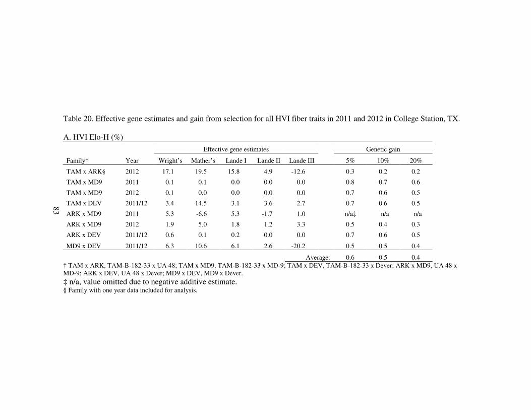
83

Table 20. Effective gene estimates and gain from selection for all HVI fiber traits in 2011 and 2012 in College Station, TX.

A. HVI Elo-H (%)

Effective gene estimates Genetic gain

Family† Year Wright’s Mather’s Lande I Lande II Lande III 5% 10% 20%

TAM x ARK§ 2012 17.1 19.5 15.8 4.9 -12.6 0.3 0.2 0.2

TAM x MD9 2011 0.1 0.1 0.0 0.0 0.0 0.8 0.7 0.6

TAM x MD9 2012 0.1 0.0 0.0 0.0 0.0 0.7 0.6 0.5

TAM x DEV 2011/12 3.4 14.5 3.1 3.6 2.7 0.7 0.6 0.5

ARK x MD9 2011 5.3 -6.6 5.3 -1.7 1.0 n/a‡ n/a n/a

ARK x MD9 2012 1.9 5.0 1.8 1.2 3.3 0.5 0.4 0.3

ARK x DEV 2011/12 0.6 0.1 0.2 0.0 0.0 0.7 0.6 0.5

MD9 x DEV 2011/12 6.3 10.6 6.1 2.6 -20.2

0.5 0.5 0.4

Average: 0.6 0.5 0.4

† TAM x ARK, TAM-B-182-33 x UA 48; TAM x MD9, TAM-B-182-33 x MD-9; TAM x DEV, TAM-B-182-33 x Dever; ARK x MD9, UA 48 x

MD-9; ARK x DEV, UA 48 x Dever; MD9 x DEV, MD9 x Dever.

‡ n/a, value omitted due to negative additive estimate. § Family with one year data included for analysis.

84

Table 20. Continued.

B. HVI Str-H (kN m kg-1

)

Effective gene estimates Genetic gain

Family† Year Wright’s Mather’s Lande I Lande II Lande III 5% 10% 20%

TAM x ARK§ 2012 -11.0 8.5 -7.3 2.1 -1.3 7.9 6.8 5.4

TAM x MD9 2011 0.1 0.1 0.1 0.0 -0.1 45.6 39.0 31.0

TAM x MD9 2012 -1.4 0.0 0.0 0.0 0.0 13.9 11.8 9.4

TAM x DEV 2011 0.3 0.4 0.1 0.1 0.1 35.7 30.5 24.3

TAM x DEV 2012 0.1 0.1 0.0 0.0 0.1 11.1 9.5 7.5

ARK x MD9 2011 -5.3 8.3 -5.1 2.1 -1.1 8.7 7.4 5.9

ARK x MD9 2012 2.7 49.8 2.5 12.4 1.4 3.1 2.7 2.1

ARK x DEV 2011 1.2 4.7 1.2 1.2 1.2 13.8 11.8 9.4

ARK x DEV 2012 1.2 1.8 1.0 0.4 -3.1 30.6 26.1 20.8

MD9 x DEV 2011 -0.2 0.1 -0.1 0.0 0.0

21.0 18.0 14.3

MD9 x DEV 2012 0.6 0.2 0.1 0.0 -0.1 12.7 10.8 8.6

Average: 18.6 15.9 12.6

† TAM x ARK, TAM-B-182-33 x UA 48; TAM x MD9, TAM-B-182-33 x MD-9; TAM x DEV, TAM-B-182-33 x Dever; ARK x MD9, UA 48 x

MD-9; ARK x DEV, UA 48 x Dever; MD9 x DEV, MD9 x Dever.

§ Family with one year data included for analysis.

85

Table 20. Continued.

C. HVI UHML (mm)

Effective gene estimates Genetic gain

Family† Year Wright’s Mather’s Lande I Lande II Lande III 5% 10% 20%

TAM x ARK§ 2012 7.7 9.7 7.1 2.4 -7.6 1.4 1.2 1.0

TAM x MD9 2011/12 1.5 0.7 1.5 0.2 -0.2 1.0 0.9 0.7

TAM x DEV 2011/12 2.4 7.5 2.1 1.9 2.4 1.2 1.0 0.8

ARK x MD9 2011 7.6 -92.1 7.5 -23.0 3.2 n/a‡ n/a n/a

ARK x MD9 2012 -5.7 -7.8 -5.7 -2.0 6.3 n/a n/a n/a

ARK x DEV 2011 -3.5 3.2 -2.1 0.8 -0.5 0.6 0.5 0.4

ARK x DEV 2012 1.0 0.4 0.3 0.1 -0.3 2.2 1.9 1.5

MD9 x DEV 2011 1.7 2.9 1.7 0.7 -4.5

1.2 1.0 0.8

MD9 x DEV 2012 1.2 2.6 1.1 0.7 2.9 1.6 1.3 1.1

Average: 1.3 1.1 0.9

† TAM x ARK, TAM-B-182-33 x UA 48; TAM x MD9, TAM-B-182-33 x MD-9; TAM x DEV, TAM-B-182-33 x Dever; ARK x MD9, UA 48 x

MD-9; ARK x DEV, UA 48 x Dever; MD9 x DEV, MD9 x Dever.

‡ n/a, value omitted due to negative additive estimate. § Family with one year data included for analysis.

86

Table 20. Continued.

D. HVI UI (%)

Effective gene estimates Genetic gain

Family† Year Wright’s Mather’s Lande I Lande II Lande III 5% 10% 20%

TAM x ARK§ 2012 -1.2 12.2 -0.9 3.0 -0.4 0.2 0.2 0.2

TAM x MD9 2011/12 0.1 0.2 0.1 0.0 -0.4 1.9 1.6 1.3

TAM x DEV 2011 2.2 -177.0 2.0 -44.2 1.0 n/a‡ n/a n/a

TAM x DEV 2012 0.7 2.1 0.6 0.5 0.7 1.1 0.9 0.7

ARK x MD9 2011/12 -0.7 -2.3 -0.3 -0.6 -0.2 n/a n/a n/a

ARK x DEV 2011/12 3.4 0.6 1.0 0.2 -0.2 1.0 0.8 0.7

MD9 x DEV 2011/12 0.4 0.6 0.2 0.2 0.2

1.1 0.9 0.7

Average: 1.1 0.9 0.7

† TAM x ARK, TAM-B-182-33 x UA 48; TAM x MD9, TAM-B-182-33 x MD-9; TAM x DEV, TAM-B-182-33 x Dever; ARK x MD9, UA 48 x

MD-9; ARK x DEV, UA 48 x Dever; MD9 x DEV, MD9 x Dever.

‡ n/a, value omitted due to negative additive estimate. § Family with one year data included for analysis.

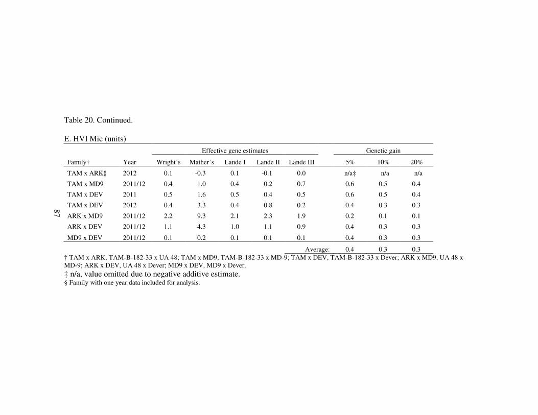
87

Table 20. Continued.

E. HVI Mic (units)

Effective gene estimates Genetic gain

Family† Year Wright’s Mather’s Lande I Lande II Lande III 5% 10% 20%

TAM x ARK§ 2012 0.1 -0.3 0.1 -0.1 0.0 n/a‡ n/a n/a

TAM x MD9 2011/12 0.4 1.0 0.4 0.2 0.7 0.6 0.5 0.4

TAM x DEV 2011 0.5 1.6 0.5 0.4 0.5 0.6 0.5 0.4

TAM x DEV 2012 0.4 3.3 0.4 0.8 0.2 0.4 0.3 0.3

ARK x MD9 2011/12 2.2 9.3 2.1 2.3 1.9 0.2 0.1 0.1

ARK x DEV 2011/12 1.1 4.3 1.0 1.1 0.9 0.4 0.3 0.3

MD9 x DEV 2011/12 0.1 0.2 0.1 0.1 0.1

0.4 0.3 0.3

Average: 0.4 0.3 0.3

† TAM x ARK, TAM-B-182-33 x UA 48; TAM x MD9, TAM-B-182-33 x MD-9; TAM x DEV, TAM-B-182-33 x Dever; ARK x MD9, UA 48 x

MD-9; ARK x DEV, UA 48 x Dever; MD9 x DEV, MD9 x Dever.

‡ n/a, value omitted due to negative additive estimate. § Family with one year data included for analysis.

88

CHAPTER VI

SUMMARY OF GENERATION MEANS ANALYSIS

All six generations within each family exhibited variability in Elo-H values with

the exception of the TAM x MD9 family due to similar Elo-H values for both parents

used for the family (Table 15). Experimental line DEV, with parental Elo-S of 7.6%,

when used as a parent, consistently exhibited high Elo-H ranging from 9.29% in the

TAM x DEV family in 2011/12 to 9.70% in the ARK x DEV family in 2012. The

efficacy of the DEV experimental line as a potential donor for fiber Elo-H was shown

further by the high F2 means when crossed with diverse genotypes of upland cotton

genotypes used in this study. When comparing Elo-H means across years by family

(when applicable), generation means were, in general, higher in 2012 than in 2011. Such

upward trend was observed in fiber UHML and to a lesser degree, in fiber and UI

suggesting that 2012 was a more conducive year for cotton quality (Table 16).

As determined by the ABCD scaling test, no significant epistatic interaction was

observed in all families as the three parameter model explained more than 95% of total

variations observed in fiber Elo-H, Str-H, UI and Mic (Table 18). Significant non- allelic

interactions were observed in UHML for TAM x ARK in 2012. Additive gene effects

were the only significant gene effects detected for fiber Elo-H in this study, which

corresponded well with multiple previous studies by May and Green, (1994), Miller and

Rawling, (1967), and Quisenberry, (1975). Elo-H additive variance explained a much

larger portion of the total genotypic variation than did dominance variance (Table 19).

89

High numbers of effective factors for Elo-H were identified for the TAM x ARK family

in 2012 and the TAM x DEV family in 2011/12 with Mather’s model. Since the parent

TAM was present in both families, and low levels of effective factors were identified in

the ARK x DEV family, it is tempting to conclude that TAM had a distinctive gene pool

for Elo-H but not different than that of MD9 due to the low to zero effective factors

between the TAM and MD9. In the same context, ARK and DEV may be carrying

similar genes but on opposite ends as the high parental Elo-H of DEV was nullified by

ARK (Table 20).

In conclusion, there was more variation in fiber Elo-H than fiber Str-H, UHML,

UI or Mic in all families used in this study as indicated by the means (Table 16) and

effective factor estimates (Table 20). All parental materials in this study were elite

materials representing major cotton breeding programs in the U.S., and should therefore,

have minimal variations within genotypes for Str-H, UHML, UI and Mic. However, due

to the absence of standardized Elo-H measurements and the lack of emphasis on Elo-H

during the development of these parental genotypes, Elo-H may vary considerably

among these breeding programs. This means that selection in Elo-H within these

families that are stable for all other important fiber traits could still result in significant

gain.

90

CHAPTER VII

CONCLUSIONS

Diallel study for fiber elongation with five representative parental genotypes has

demonstrated that additive gene action in fiber elongation far outweighs the dominance

gene effects. Comparing the mean squares of GCA and SCA for fiber elongation, GCA

explained many folds more of the total variations observed in the study. This would

suggest that fiber elongation is a trait that can be easily selected for and improved using

traditional pedigree breeding scheme. The study has determined two of the seven

parental genotypes used, i.e. PSC and DEV to be superior combiners for fiber

elongation. These two parents may serve as good sources of fiber elongation for future

breeding efforts as they also represent two very significant breeding environments in the

U.S. When elongation was measured using the Stelometer, elongation values were

consistently lower than that of HVI. Both HVI and Stelometer reported very low C.V.s

in elongation, suggesting that despite all the differences in instrumentations and testing

protocols, the two instruments are very precise. Such observation was further testified by

the high correlation between Elo-H and Elo-S in 2010 and 2011.

91

Data reported by generation means analysis herein supports conclusions by May

and Green, (1994), Miller and Rawlings, (1967) and Quisenberry, (1975) that fiber

elongation is primarily governed by additive gene action and to a lesser degree by

dominance gene action. Epistatic gene effects were insignificant for fiber elongation as

indicated by the ABCD scaling test. Based on the number of effective factors identified

in this study, there are two distinctive gene pools for fiber elongation, one represented by

TAM and MD9 and the other by ARK and DEV. For breeders interested in breeding for

high elongation upland cotton, crossing between these two gene pools may help to

diversify genetics in fiber elongation. For all families, larger variation was observed for

fiber elongation as compared to the other fiber traits included in this study. With the

representative parental genotypes used, this may be a good indication that fiber

elongation is still segregating in these otherwise stable genotypes. This would also mean

that reselection in current U.S. upland cultivars could result in significant gain in

elongation.

92

REFERENCES

Al-Rawi, K.M., and R.J. Kohel. 1969. Diallel analysis of yield and other agronomic

characters in Gossypium hirsutum L. Crop Sci. 10:82-85.

Al-Rawi, K.M., and R.J. Kohel. 1970. Gene action in the inheritance of fiber properties

in intervarietal diallel crosses of upland cotton, Gossypium hirsutum L. Crop Sci.

10:82-85.

Ali, M.A., I.A. Khan, S.I. Awan, S. Ali, and S. Niaz. 2008. Genetics of fiber quality

traits in cotton (Gossypium hirsutum L.). Australian J. Crop Sci. 2:10-17.

ASTM. 2005. Standard test methods for measurement of cotton fibers by high volume

instruments (D5867 – 05). p. 1-8. DOI:10.1520/ D5867-05. American Society for

Testing and Materials, West Conshohocken, PA.

ASTM. 2012. Standard test method for breaking strength and elongation of cotton fibers

(flat bundle method) (D1445/D1445M – 12). p. 1-8. DOI: 10.1520/

D1445_D1445M-12. American Society for Testing and Materials, West

Conshohocken, PA.

Anderson, V.L., and O. Kempthorne. 1954. A model for the study of quantitative

inheritance. Genetics 39:883-898.

Anguiar, P.A., J.C.V. Penna, E.C. Freire, and L.C. Melo. 2007. Diallel analysis of

upland cotton cultivars. Crop Breeding and Appl. Biotechnology 7:353-359.

Bargeron III, J.D. 1998. Cotton elongation measurement using high volume instruments.

Am. Soc. Agric. Eng. 41:1583-1587.

Benson, N.R., F.M. Bourland, W.C. Robertson, J.M. Hornbeck, and F.E. Groves. 2000.

Arkansas Cotton Variety Tests. AAES Research Series 481:1-35.

Benzina, H., E. Hequet, N. Abidi, J. Gannaway, J.-Y. Drean, and O. Harzallah. 2007.

Using fiber elongation to improve genetic screening in cotton breeding programs.

Textile Res. J. 77:770-778.

Bernardo, R. 2002. Breeding for quantitative traits in plants. Stemma Press. Woodbury,

MN.

Berger, G., S. Hague, and C.W. Smith. 2012. Diallel analysis of fiber traits for extra-

long staple cotton progeny. Crop Sci. 52:683-689.

93

Bourland, F.M., and D.C. Jones. 2012. Registration of ‘UA 48’ cultivar. J. Plant

Registrations 6:15-18.

Braden, C.A., C.W. Smith, and E. Hequet. 2009. Combining ability for fiber length in

near-long-staple upland cotton. Crop Sci. 49:756-762.

Bradow, J.M., and G.H. Davidonis. 2000. Quantification of fiber quality and the cotton

production-processing interface: a physiologist’s perspective. J. Cotton Sci. 4:34-

64.

Campbell, B.T., and M.A. Jones. 2005. Assessment of genotype x environment

interactions for yield and fiber quality in cotton performance trials. Euphytica

144: 69-78.

Cantrell, R.G., C.L. Roberts, and C. Waddell. 2000. Registration of ‘Acala 1517-99’

cotton. Crop Sci. 40:1200-1201.

Cheatham, C.L., J.N. Jenkins, J.C. McCarty, Jr., C.E. Watson, and J. Wu. 2003. Genetic

variances and combining ability of crosses of American cultivars, Australian

cultivars, and wild cottons. J. Cotton Sci. 7:16-22.

Cotton Incorporated. 2012. Rating of fiber properties. [Online] Available at:

http://www.cottoninc.com/fiber/quality/US-Fiber-Chart/Ratings-Of-Fiber-

Properties/ (accessed January 2012; verified 2 Apr. 2013). Cotton Incorporated,

Cary, NC.

Cui, X., M.W. Suh, and P.E. Sasser. 2003. Estimating single fiber tensile properties from

the load-elongation curves of slack bundles. Textile Res. J. 73:1066-1070.

Dever, J. 2012. Personal communication. Development of high elongation cotton lines.

Texas A&M AgriLife Research, Lubbock, TX.

Dudley, J.W., and R.J. Lambert. 2004. 100 generations of selection for oil and protein in

corn. Plant Breed. Rev. 24:79-110.

Egle, C.J., and J.N. Grant. 1970. Interrelations of structural and physical properties of

untreated cottons. Textile Res. J. 40:158-168.

Endrizzi, J.E. 1962. The diploid-like cytological behavior of tetraploid cotton. Evolution

16:325-329.

Falconer, D.S. 1960. Introduction to quantitative genetics. The Ronald Press Company,

New York, NY.

94

Faulkner, W.B., E.F. Hequet, J. Wanjura, and R. Boman. 2012. Relationships of cotton

fiber properties to ring-spun yarn quality on selected high plains cotton. Textile

Res. J. 82: 400-414.

Fehr, W.R. 1991. Principle of Cultivar Development. Dept. of Agronomy, Iowa State

University, IA.

Foulk, J.A. 2007. Commercial cotton variety spinning study HVI and AFIS spinning

relationship. Beltwide Cotton Conference, New Orleans, LA. P. 1808-1814.

Gamble, E.E. 1962. Gene effects in corn (Zea Mays L.) I. Separation and relative

importance of gene effects for yield. Can. J. Plant Sci. 42:339-348.

Geng, S., Q. Zhang, and D.M. Bassett. 1987. Stability in yield and fiber quality of

California cotton. Crop Sci. 27:1004-1010.

Gill, J.L., and E.L. Jensen. 1968. Probability of obtaining negative estimates of

heritability. Biometrics 517-526.

Green, C.C.,and T.W. Culp. 1990. Simultaneous improvement of yield, fiber quality, and

yarn strength in upland cotton. Crop Sci. 30:66-69.

Gregory, K., E.H. Ng, C.W. Smith, E. Hequet, and S. Hague. 2012. Fiber and yarn

performance of upland cotton with improved fiber bundle strength. Crop Sci.

52:1-7.

Griffing, B. 1956a. A generalized treatment of the use of diallel crosses in quantitative

inheritance. Heredity 10:31-50.

Griffing, B. 1956b. Concept of general and specific combining ability in relation to

diallel crossing systems. Aust. J. Biol. Sci. 9:463-493.

Gusmini, G., T.C. Wehner, and S.B. Donaghy. 2007. SASQuant: A SAS software

program to estimate genetic effects and heritabilities of quantitative traits in

populations consisting of 6 related generations. Heredity 98:345-350.

Hallauer, A.R., and J.B. Miranda. 1988. Quantitative genetics in maize breeding. 2nd

ed.

Iowa State University Press, Ames, IA.

Hayman, B.I. 1958. The separation of epistatic from additive and dominance variation in

generation means. Heredity 12:371-390.

95

Hayman, B.I. 1960. The separation of epistatic from additive and dominance variation in

generation means. II. Genetica 31:133-146.

Hayman, B.I., and K. Mather. 1955. The description of genetic interaction in continuous

variation. Biometrics 11:69-82.

Hertel, K.L. 1953. The Stelometer, it measures fiber strength and elongation. Textile

World 103:97-260.

Hertel, K.L. 1955. Stelometer fiber tester. U.S. patent no. 2,706,403.

Hequet, E. F. 2012. Personal communication. Regression method for elongation

measurement using stelometer. Fiber and Bio-polymer Research Institute,

Lubbock, TX.

Hequet, E. F., B. Wyatt, N. Abidi, and D. Thibodeaux. 2006. Creation of a set of

reference materials for cotton fiber maturity measurements. Textile Res. J. 76(7):

576-586.

ITMF. 2012. International Cotton Industry Statistics-ICIS [Online] Available at:

http://www.itmf.org/wb/pages/home/publications/detail.php?id=2 (accessed May

2012; verified 2 Apr. 2013). International Textile Manufacturers Federation,

Zurich, Switzerland.

Iqbal, M.J., O.U.K. Reddy, K.M. El-Zak, and A.E. Pepper. 2001. A genetic bottleneck in

the evolution under domestication of upland cotton (G. hirsutum) examined using

DNA finger printing. Theor. Appl. Genet. 103: 547-554.

Jenkins, J.N., J.C. McCarthy Jr., J. Wu, and O.A. Gutierrez. 2009. Genetic variance

components and genetic effects among eleven diverse upland cotton lines and

their F2 hybrids. Euphytica 167: 397-408.

Joy, K., C.W. Smith, E. Hequet, S. Hague, P.S. Thaxton, and C. Souder. 2010. Fiber

properties and mini-spun yarn performance of extra long staple upland cotton. J.

Cotton Sci. 14:82-90.

Kearsey, M.J., and H.S. Pooni. 1996. The genetical analysis of quantitative traits.

Chapman and Hall, London, U.K.

Kempthorne, O. 1957. An introduction to genetic statistics. Chapman and Hall, London,

U.K.

96

Khadi, B.M., V. Santhy, and M.S. Yadav. 2010. Cotton: an introduction. p. 1-14. In U.B.

Zehr (ed.) Cotton, biotechnology in agriculture and forestry 65. Springer-Verlag

Berlin Heidelberg.

Kimber, G. 1961. Basis of the diploid-like meiotic behavior of polyploidy cotton. Nature

19:98-100.

Lande, R. 1981. The minimum number of genes contributing to quantitative variation

between and within populations. Genetics 99:541-553.

Lee, J.A., P.A. Miller, and J.O. Rawlings. 1967. Interaction of combining ability effects

with environments in diallel crosses of upland cotton (Gossypium hirsutum L.)

Crop Sci. 7:477-481.

Liu, J., H. Yang, and Y.-L. Hsieh. 2001. Variations of mature cotton fiber tensile

properties: association with seed position and fiber length. Textile Res. J. 12:

1079-1086.

Liu, J., H. Yang, and Y.-L. Hsieh. 2005. Distribution of single fiber tensile properties of

four cotton genotypes. Textile Res. J. 75:117-122.

Luckett, D.J. 1989. Diallel analysis of yield components, fiber quality and bacterial

blight resistance using spaced plants of cotton. Euphytica 44:11-21.

Lush, J.L. 1945. Animal breeding plans. The Collegiate Press, Inc. Ames, IA.

Marek, T., and D. Bordovsky. 2006. Performance of ten cotton varieties in northern

Texas high plains. Texas J. Agri. Nat. Res. 19:48-61.

Mather, K. 1949. Biometrical genetics. Dover Publication Inc., London, U.K.

Mather, K. 1973. Genetical structure of populations. Chapman and Hall, London, U.K.

Mather, K., and J. L. Jinks. 1977. Introduction to biometrical genetics. Chapman and

Hall, London, U.K.

Mather, K., and J.L. Jinks. 1982. Biometrical genetics. The study of continuous

variation. 3rd

ed. Chapman and Hall, London, U.K.

May, O.L. 1999. Genetic variation in fiber quality. In A.S. Basra (ed.) Cotton fibers.

Food Products Press, Binghamton, NY.

May, O.L., and C.C. Green. 1994. Genetic variation for fiber properties in Elite Pee Dee

cotton populations. Crop Sci. 34:684-690.

97

May, O.L., and G.M. Jividen. 1999. Genetic modification of cotton fiber properties as

measured by single- and high volume instruments. Crop Sci. 39:328-333.

May, O.L., and K.E. Lege. 1999. Development of the world cotton industry. P65-97. In

C.W. Smith, J.T. Cothren (eds.) Cotton origin, history, technology and

production. John Wiley & Sons Inc., New York.

May, O.L., and R.A. Taylor. 1998. Breeding cottons with higher yarn tenacity. Textile

Res. J. 68:302-307.

May, O.L., R.F. Davis, and S.H. Baker. 2001. Registration of GA 161 cotton. Crop Sci.

41:1995

Meredith, R. 1945. The tensile behavior of raw cotton and other textile fibers. J. Textile

Inst. Transactions. 36:107-130.

Meredith, W.R, T.W. culp, K.Q. Robert, G.F. Ruppenicker, W.S. Anthony, and J.R.

Williford. 1991. Determining future cotton variety fiber quality objectives.

Textile Res. J. 61:715-720.

Meredith, W.R., and W.S. Nokes. 2011. Registration of MD 9ne and MD 25 high-fiber-

quality germplasm lines of cotton. J. Plant Registrations 5: 202-206.

Meyer, V.G. 1974. Interspecific cotton breeding. Econ. Bot. 28:56-60.

Miller, P.A., and J.O. Rawlings. 1967. Selection for increased lint yield and correlated

responses in upland cotton, Gossypium hirsutum L. Crop Sci. 7:637-640.

Moll, R., and C.W. Stuber. 1974. Quantitative genetics- empirical results relevant to

plant breeding. Adv. Agron. 26-277-313.

National Cotton Council. 2012. CCC loan information [Online]. Available at:

http://www.cotton.org/econ/govprograms/cccloan/index.cfm (accessed May

2012; verified 2 Apr. 2013). National cotton council, Memphis, TN.

Nzaramba, M.N., A.L. Hale, D.C. Scheurig, and J.C. Miller Jr. 2005. Inheritance of

antioxidant activity and its association with seedcoat color in cowpea. J. Amer.

Soc. Hort. Sci. 130:386-391.

Orr, R.S., A.W. Burgis, L.B. DeLuca, and J.N. Grant. 1961. The role of spiral structure

in untreated and treated cottons. Textile Res. J. 31:302-310.

98

Orr, R.S., L.C. Weiss, and J.N. Grant. 1955. The relation of single-fiber to flat-bundle

strength and elongation of cotton. Textile Res. J. 25:939-946.

Palmer, A.W. 1924. The commercial classification of American cotton. Circ. 278.

USDA, Washington, DC.

Paterson, A.H., Y. Saranga, M. Menz, C.-X. Jiang, and R.J. Wright. 2003. QTL analysis

of genotype x environment interactions affecting cotton fiber quality. Theor.

Appl. Genet. 106:384-396.

Pavasia, M.J., P.T. Shukla, and U.G. Patel. 1999. Combining ability analysis over

environments for fiber characters in upland cotton. Ind. J. Genet. 59:77-81.

PCCA. 2012. PCCA’s history [Online] Available at:

http://www.pcca.com/corporate/pccahistory.asp (accessed May 2012; verified 2

Apr. 2013). Plains Cotton Cooperative Association, Lubbock, TX.

Pooni, H.S., D.T. Coombs, P.S. Virk, and J.L. Jinks. 1987. Detection of epistasis and

linkage of interacting genes in the presence of reciprocal differences. Heredity

58:257-266.

Pressley, E.H. 1942. A cotton fiber strength tester. A.S.T.M. Bulletin 118:13.

Preston, R.D. 1974. The physical biology of plant cell walls. Chapman and Hall Ltd.

London, U.K.

Quisenberry, J.E. 1975. Inheritance of fiber properties among crosses of Acala and high

plains cultivars of upland cotton. Crop Sci. 15:202-205.

Ramey, H.H. 1999. Classing of fiber. p. 709-727. In C.W. Smith and J.T. Cothren (ed.).

Cotton origin, history, technology, and production. John Wiley & Sons, Inc. New

York.

Ramey, H.H., and P.A. Miller. 1966. Partitioned genetic variances for several characters

in a cotton population of interspecific origin. Crop Sci. 6:123-125.

Ramey, H.H., R. Lawson, and S. Worley Jr. 1977. Relationship of cotton fiber properties

to yarn tenacity. Textile Res. J. 47: 685-691.

Riley Jr., C.R. 1997. Quality measurements: Improved high volume instrument

elongation measurements. J. Cotton Sci. 1:61-71.

SAS Institute. 2011. The SAS system for Windows. Release 9.2. SAS Inst., Cary, NC.

99

SAS Institute. 2013. JMP Pro 10. SAS Inst., Cary NC.

Sasser, P.E., F.M. Shofner, Y.T. Chu, C.K. Shofner, and M.G. Townes. 1991.

Interpretations of singe fiber, bundle, and yarn tenacity data. Textile Res. J.

11:681-690.

Scholl, R.L., and P.A. Miller. 1976. Genetic association between yield and fiber strength

in upland cotton. Crop Sci. 16: 780-783.

Schwartz, B.M., and C.W. Smith. 2008. Genetic gain in fiber properties of upland cotton

under varying plant densities. Crop Sci. 48:1321-1327.

Shofner, F.M., Y.T. Chu, C.K. Shofner, and M.G. Townes. 1991. Interpretations of

single fiber, bundle, and yarn tenacity data. Textile Rex. J. 61:681-690.

Singh, M, T.H. Singh, and G.S. Chahal. 1985. Genetic analysis of some seed quality

characters in upland cotton. Theor. Appl. Genet. 71:126-128.

Singh, R.K., and B.D. Chaudary. 1977. Biometrical methods in quantitative genetics

analysis. Kalyani Publishers, New Delhi, India.

Smith, C.W. 2003. Registration of TAM 94L-25 and TAM 94J-3 germplasm lines of

upland cotton with improved fiber length. Crop Sci. 43:742–743

Smith, C.W. 1999. Production statistics. p435-449. In C.W. Smith, J.T. Cothren (eds.)

Cotton origin, history, technology and production. John Wiley & Sons Inc., New

York.

Smith, C.W., P.S. Thaxton, S.Hague, E. Hequet, and D. Jones. 2008a. Registration of

TAM 01E-22 upland cotton germplasm line with improved fiber bundle strength.

Germplasm 2:129-131.

Smith, C.W., S. Hague, E. Hequet, P.S. Thaxton, and I.N. Brown. 2008b. Development

of extra-long staple upland cotton. Crop Sci. 48:1823-1831.

Smith, C.W., S. Hague, P.S. Thaxton, E. Hequet, and D. Jones. 2009. Eight extra long

staple upland cotton germplasms. J. Plant Registrations 3:81.

Suh, M.W., X. Cui, and P.E. Sasser. 1993. Interpretation of HVI bundle tensile

properties through single fiber test results- effects of fiber slack. Proc. Beltwide

Cotton Conference. 1101-1104.

Suh, M.W., X. Cui, and P.E. Sasser. 1994. New understanding on HVI tensile data based

in Mantis single fiber test results. Proc. Beltwide Cotton Conference. 1400-1403.

100

Tang, B., J.N. Jenkins, C.E. Watson, J.C. McCarty, and R.G. Creech. 1996. Evaluation

of genetic variances, heritabilites, and correlations for yield and fiber traits

among cotton F2 hybrid populations. Euphytica 91:315-322.

Tang, B, J.N. Jenkins, J.C. McCarthy, and C.E. Watson. 1993. F2 hybrids of host plant

germplasm and cotton cultivars: II. Heterosis and combining ability for fiber

properties. Crop Sci. 33:706-710.

Tchiagam, J.B.N., E. Youmbi, N.Y. Njintang, J.M. Bell, and A.N. Maina. 2011.

Generation means analysis of seed sucrose content in cowpea (Vigna unguiculata

L. Walp.). Asian J. of Agri. Sci. 3:475-480.

Tensometric Company Ltd. UT350®

. Material testing machine. Lancashire, U.K.

Thibodeaux, D.P., J.J. Hebert, N.S. Abd. El-Gawad, and J.S. Moraitis. 1998. Quality

measurements- relating bundle strength to Mantis single fiber strength

measurements. J. Cotton Sci. 2:62-67.

Toman Jr., J., and D.G. White. 1993. Inheritance of resistance to anthracnose stalk rot of

corn. Phytopathology 83:981-986.

USDA. 2013. International calibration cotton standard. Agriculture and marketing

service- cotton program. Memphis, TN.

Uster. 2012a. HVI 1000®

. High volume instrument. Knoxville, TN.

Uster. 2012b. Stelometer 654®

. Stelometer. Knoxville, TN.

Verhalen, L.M., W.C. Morrison, B.A. Al-Rawi, K.-C. Fun, and J.C. Murray. 1970. A

diallel analysis of several agronomic traits in upland cotton (Gossypium hirsutum

L.). Crop Sci. 11: 92-96.

Warner, J.N. 1952. A method for estimating heritability. Agron. J. 44:427-430.

White, T.G., and R.J. Kohel. 1964. A diallel analysis of agronomic characters in selected

lines of Gossypium hirsutum L. Crop Sci. 4:254-257.

Wilson, F.D., and R.L. Wilson. 1975. Breeding potentials of non- cultivated cottons.-I.

Some agronomic and fiber properties of selected parents and their F1 hybrids.

Crop Sci. 15:763-766.

Wright, S. 1968. The genetics of quantitative variability. Evolution and the genetics of

populations. 2nd

ed. Vol. 1. University of Chicago Press, IL.

101

Wendel, J.F., C.L. Brubaker, and A.E. Pervical. 1992. Genetic diversity in Gossypium

hirsutum and the origin of upland cotton. Am. J. Bot. 79:1291-1310.

Wendel, J.F., and R.C. Cronn. 2003. Polyploidy and the evolutionary history of cotton.

Adv. Agron. 78:139-186.

Zhang, J.F., C. Waddell, C. Sengupta-Gopalan, C. Potenza, and R.G. Cantrell. 2007.

Diallel analysis of root-knot nematode resistance based on galling index in

upland cotton. Plant Breed. 126:164-168.

Zhang, Y., M.S. Kang, and K.R. Lamkey. 2005. Diallel-SAS05: A comprehensive

program for Griffing’s and Gardner-Eberhart Analyses. Agron. J. 97:1097-1106.