genetic algorithm-based feature set partitioning for ... · 1 genetic algorithm-based feature set...
TRANSCRIPT
1
Genetic Algorithm-based Feature Set Partitioning for Classification Problems
Lior Rokach
Department of Information System Engineering Ben-Gurion University of the Negev
Keywords Feature Set-Partitioning, Feature Selection, Genetic Algorithm, Ensemble Learning
Abstract Feature set partitioning generalizes the task of feature selection by partitioning the feature set into subsets of features that are collectively useful, rather than by finding a single useful subset of features. This paper presents a novel feature set partitioning approach that is based on a genetic algorithm. As part of this new approach a new encoding schema is also proposed and its properties are discussed. We examine the effectiveness of using a Vapnik-Chervonenkis dimension bound for evaluating the fitness function of multiple, oblivious tree classifiers. The new algorithm was tested on various datasets and the results indicate the superiority of the proposed algorithm to other methods.
1. Introduction and Motivation
An inducer aims to build a classifier (also known as a classification model) by learning from a set of pre-classified instances. The classifier can then be used for classifying unlabelled instances. It is well known that the required number of labeled instances for supervised learning increases as a function of dimensionality [1]. Fukunaga [2] showed that the required number of training instances for a linear classifier is linearly related to the dimensionality and for a quadratic classifier to the square of the dimensionality. In terms of nonparametric classifiers such as decision trees, the situation is even more severe. It has been estimated that, as the number of dimensions increases, the training set size needs to increase exponentially in order to obtain an effective estimate of multivariate densities [3].
Bellman [4], while working on complicated signal processing problems, was the first to define this phenomenon as the "curse of dimensionality." Techniques that are efficient in low dimensions, such as decision trees inducers, fail to provide meaningful results when the number of dimensions increases beyond a 'modest' size. Furthermore, humans are better able to comprehend smaller classifiers involving fewer features (probably less than 10). Smaller classifiers are also more appropriate for user-driven data mining techniques such as visualization.
In this paper we propose a way to avoid the curse of dimensionality by decomposing the original feature set into several mutually exclusive subsets. This is known as feature set partitioning and may be regarded as a generalization of the feature selection task. Moreover, feature set partitioning is regarded as a specific case of ensemble methodology in which members use disjoint feature subsets, i.e., every classifier in the ensemble is trained on a different projection of the original training set.
As an example of some of the aspects involved in feature set partitioning, consider a training set containing data about health insurance policyholders. Each policyholder is characterized by four features: Asset Ownership, Education (years), Car Engine Volume (in cubic centimeters) and Employment Status. The target feature (i.e., the label) describes whether a specific policyholder was willing to purchase complementary insurance and what type of complementary insurance she was willing to buy. A possible feature set partitioning ensemble for resolving the question includes two decision trees. The first decision tree uses the features Asset Ownership and Volume, while the second uses the features Employment Status and Education.
The aim of this work is to examine whether genetic algorithm-based feature set partitioning can improve classification performance. We propose a new encoding schema. Theoretical results are used to explain why this new encoding is more suitable than more straightforward encoding schemas. In order to

2
avoid long training time, a Vapnik-Chervonenkis dimension bound for multiple oblivious trees evaluates the fitness function. A caching mechanism is suggested in order to reduce further the computational cost of the genetic algorithm. The superiority of the suggested algorithm to other methods is illustrated on various datasets.
The rest of this paper is organized as follows: Section 2 reviews related works in the field of feature selection, feature set partitioning, and the usage of ensemble of feature selectors. Section 3 formulates the problem. Section 4 presents a new algorithm for solving the problem discussed here. Section 5 reports the experiments carried out to examine the new algorithm. Finally, Section 6 concludes the work and presents suggestions for further research in the field. Proofs for the theoretical claims presented in this paper appear in the appendix. 2. Related Works In this section we briefly review some of the central issues that have been addressed, and their treatment in the literature. The related work described in this section falls into three categories:
• First, we discuss three feature oriented tasks (namely feature selection, feature set partitioning, and feature subset based ensemble) in pattern recognition and the relations among them.
• Then, we survey the usage of genetic algorithms for solving the above-mentioned tasks. • The oblivious decision tree and it usage for solving feature selection problems.
Finally, in the light of previous work, we summarize the original contribution of this paper. 2.1 Feature selection
Most methods of dealing with high dimensionality focus on feature selection techniques, i.e., selecting a single subset of features upon which the inducer will run, while ignoring the rest. The selection of the subset can be done manually using prior knowledge to identify irrelevant variables or feature selection algorithms. In the last decade, many researchers have shown increased interest in feature selection, and consequently many algorithms have been proposed, with some demonstrating remarkable improvements in accuracy. Since the subject is too wide to survey here, the reader is referred to Ref. [5] for further reading.
Despite their popularity, there are several drawbacks to using feature selection methodologies in order to overcome the dimensionality curse:
• The assumption that a large set of input features can be reduced to a small subset of relevant features is not always true; in some cases the target feature is actually affected by most of the input features and removing features will cause a significant loss of important information.
• The outcome (i.e., the subset) of many algorithms for feature selection (for example, almost any of the algorithms that are based on the wrapper methodology) is strongly dependent on the training set size. That is, if the training set is small, the size of the reduced subset will be small also. Consequently, relevant features might be lost. Accordingly, the induced classifiers might achieve a lower degree of accuracy compared to classifiers that have access to all relevant features.
• In some cases, even after eliminating a set of irrelevant features, the researcher is left with a relatively large number of relevant features.
• The backward elimination strategy that some methods implement is extremely inefficient for working with large-scale databases, where the number of original features is greater than 100.
2.2 Feature subset-based ensemble methods Ensemble methodology, which builds a predictive classifier by integrating multiple classifiers, can be
used to improve prediction performance. During the past few years, experimental studies have shown that combining the outputs of multiple classifiers reduces the generalization error [6]. Ensemble methods are very effective, mainly due to the phenomenon that various types of classifiers have different “inductive biases” [7]. Indeed, ensemble methods can effectively make use of such diversity to reduce the variance-error [8] without increasing the bias-error.

3
Bagging [9] and AdaBoost [10] are popular implementations of the ensemble methodology. Bagging employs bootstrap sampling to generate several training sets and then trains a classifier from each generated training set. Note that, since sampling with replacement is used, some of the original instances may appear more than once in the same generated training set and some may not be included at all. The classifier predictions are often combined via majority voting. AdaBoost sequentially constructs a series of classifiers, where the training instances that are wrongly classified by a certain classifier will get a higher weight in the training of its subsequent classifier. The classifiers’ predictions are combined via weighted voting where the weights are determined by the algorithm itself based on the training error of each classifier.
Feature subset based ensemble methods are those that manipulate the input feature set for creating the ensemble members. The idea is simply to give each classifier a different projection of the training set. Tumer and Oza [11] claim that feature subset-based ensembles potentially facilitate the creation of a classifier for high dimensionality datasets without the feature selection drawbacks mentioned above. Moreover, these methods can be used to improve the classification performance due to the reduced correlation among the classifiers. Bryll et al. [12] also indicate that the reduced size of the dataset implies faster induction of classifiers. Feature subset avoids the class under-representation which may occur in instance subsets methods such as bagging. Three popular strategies for creating feature subset-based ensembles exist: random-based, reduct-based, and performance-based.
Random-based strategy
The most straightforward techniques for creating a feature subset-based ensemble are based on random selection. Ho [13] creates a forest of decision trees. The ensemble is constructed systematically by pseudo-randomly selecting subsets of features. The training instances are projected to each subset and a decision tree is constructed using the projected training samples. The process is repeated several times to create the forest. The classifications of the individual trees are combined by averaging the conditional probability of each class at the leaves (distribution summation). Ho shows that simple random selection of feature subsets may be an effective technique because the diversity of the ensemble members compensates for their lack of accuracy.
Bay [14] proposed using simple voting in order to combine outputs from multiple KNN (K-Nearest Neighbor) classifiers, each having access only to a random subset of the original features. Each classifier employs the same number of features. Bryll et al. [12] introduce attribute bagging (AB) which combines random subsets of features. AB first finds an appropriate subset size by a random search in the feature subset dimensionality. It then randomly selects subsets of features, creating projections of the training set on which the classifiers are trained. A technique for building ensembles of simple Bayesian classifiers in random feature subsets was also examined [15]. Reduct-based strategy
A reduct is defined as the smallest feature subset which has the same predictive power as the whole feature set. By definition, the size of the ensembles that were created using reducts is limited to the number of features. There have been several attempts to create classifier ensembles by combining several reducts. Wu et al. [16] introduce the worst-attribute-drop-first algorithm to find a set of significant reducts and then combine them using naïve Bayes. Bao and Ishii [17] examine the idea of combining multiple K-nearest neighbor classifiers for text classification by reducts. Hu et al. [18] propose several techniques to construct decision forests, in which every tree is built on a different reduct. The classifications of the various trees are combined using a voting mechanism. Performance-based strategy
Cunningham and Carney [19] introduced an ensemble feature selection strategy that randomly constructs the initial ensemble. Then, an iterative refinement is performed based on a hill-climbing search in order to improve the accuracy and diversity of the base classifiers. For all the feature subsets, an attempt is made to switch (include or delete) each feature. If the resulting feature subset produces a better performance on the validation set, that change is retained. This process is continued until no further improvements are obtained. Similarly, Zenobi and Cunningham [20] suggest that the search for the

4
different feature subsets will not be guided solely by the associated error but also by the disagreement or ambiguity among the ensemble members.
Tumer and Oza [11] present a new method called input decimation (ID), which selects feature subsets based on the correlations between individual features and class labels. This experimental study shows that ID can outperform simple random selection of feature subsets.
Tsymbal et al. [21] compare several feature selection methods that incorporate diversity as a component of the fitness function in the search for the best collection of feature subsets. This study shows that there are some datasets in which the ensemble feature selection method can be sensitive to the choice of the diversity measure. Moreover, no particular measure is superior in all cases.
Gunter and Bunke [22] suggest employing a feature subset search algorithm in order to find different subsets of the given features. The feature subset search algorithm not only takes the performance of the ensemble into account, but also directly supports diversity of subsets of features.
2.3 Feature set partitioning Feature set partitioning decomposes the original set of features into several subsets and builds a
classifier for each subset. Thus, a set of classifiers is trained such that each classifier employs a different subset of the original feature set. Subsequently, an unlabelled instance is classified by combining the classifications of all classifiers.
Feature set partitioning is a particular case of feature subset-based ensembles in which the subsets are pairwise disjoint subsets. At the same time, it generalizes the task of feature selection which aims to provide a single representative set of features from which a classifier is constructed.
Several researchers have shown that the partitioning methodology can be appropriate for classification tasks with a large number of features [23, 24]. Figure 1 presents the Venn diagram of the search space of the feature-oriented tasks. As can be seen, the search space of a feature subset-based ensemble contains the search space of feature set partitioning, and the latter contains the search space of feature selection.
Figure 1: Venn diagram for the search space of the feature-oriented tasks
While mutually exclusive partitioning restricts the search space, it has some important and helpful
properties: 1. Compared to non-exclusive approaches, this approach offers a greater possibility of achieving
reduced execution time. Since most learning algorithms have computational complexity that is greater than linear in the number of features or tuples, partitioning the problem dimensionality in a mutually exclusive manner results in a decrease in computational complexity [25].
2. Since mutual exclusiveness entails using smaller datasets, the classifiers obtained for each sub-problem are smaller in size. Without the mutually exclusive restriction, each classifier can be as complicated as the classifier obtained for the original problem. Smaller classifiers contribute to comprehensibility and ease in maintaining the solution.
3. According to Ref. [14], mutually exclusive partitioning may help avoid some error correlation problems that characterize feature subset based ensembles. However, Sharkey

5
[26] argues that mutually exclusive training sets do not necessarily result in low error correlation.
4. In feature subset-based ensembles, different classifiers might generate contradictive classifications using the same features. This inconsistency in the way a certain feature can affect the final classification may increase mistrust among end-users. Accordingly, Rokach [23] claims that end-users can grasp mutually exclusive partitioning much more easily.
5. The mutually exclusive approach encourages smaller datasets which are generally more practicable. Some data mining tools can process only limited dataset sizes (for instance, when the program requires that the entire dataset be stored in the main memory). The mutually exclusive approach can ensure that data mining tools can be scaled fairly easily to large datasets [27].
The literature includes several works that deal with feature set partitioning. In one research study, the features are grouped according to the feature type: nominal value, numeric value, and text value [24]. A similar approach was also used for developing the linear Bayes classifier [28]. The basic idea consists of aggregating the features into two subsets, the first containing only the nominal and the second only the continuous features.
In another research study, the feature set was decomposed according to the target class [29]. For each class, the features with low correlation relating to that class were removed. This method was applied on a feature set of 25 sonar signals where the target was to identify the meaning of the sound (whale, cracking ice, etc.). Feature set partitioning has also been used for radar-based volcano recognition [30]. The researcher manually decomposed a feature set of 119 into 8 subsets, grouping features that were based on different image processing operations together. As a consequence, for each subset, four neural networks of different sizes were built. A new combining framework for feature set partitioning has been used for text-independent speaker identification [31].
The feature set partitioning can be achieved by grouping features based on pairwise mutual information with statistically similar features assigned to the same group [32]. For this purpose, one can use an existing hierarchical clustering algorithm. As a consequence, several feature subsets are constructed by selecting one feature from each group. A neural network is subsequently constructed for each subset. All networks are then combined.
As part of our previous work [33], a simple hill-climbing algorithm, decomposed-oblivious-gain (DOG), was proposed. This algorithm searches for the optimal partitioning using incremental oblivious decision trees. One limitation of the DOG algorithm is that it has no backtracking capabilities (for instance, removing a single feature from a subset or removing an entire subset). Furthermore, DOG begins the search from an empty partitioning structure, which may lead to subsets with a relatively small number of features. The limitations of DOG led us to consider a more profound exploration of the search space. This in turn led us to employ a GA, since an exhaustive search for large problems is impractical.
2.4 Genetic Algorithms and their Applicability in Feature Oriented Tasks
GAs are a popular type of evolutionary algorithm (EA) that have been successfully used for feature selection. Inspired by the Darwinian process of evolution, EAs are stochastic search algorithms. The motivation for applying EAs to data mining tasks is that they offer robust, adaptive search techniques that search the solution space globally [34]. When an EA is well-designed, it continually considers new solutions. Thus, it can be viewed as an "anytime" learning algorithm [35]. Such a learning algorithm should produce a good-enough solution quite quickly. It then continues to search the solution space, reporting the new "best" solution whenever one is found. Figure 2 presents a high level pseudocode of GA adapted from Ref. [34].
GAs begin by randomly generating a population of L candidate solutions. Given such a population, a GA generates a new candidate solution (population element) by selecting two of the candidate solutions as the parent solutions. This process is termed "reproduction." Generally, parents are selected randomly from the population with a bias toward the better candidate solutions. Given two parents, one or more new solutions are generated by taking some characteristics of the solution from the first parent (the "father") and some from the second parent (the "mother"). This process is termed "crossover." For

6
example, in genetic algorithms that use binary encoding of n bits to represent each possible solution, we might randomly select a crossover bit location denoted as o. Two descendant solutions could then be generated. The first descendant would inherit the first o string characteristics from the father and the remaining n-o characteristics from the mother. The second descendant would inherit the first o string characteristics from the mother and the remaining n-o characteristics from the father. This type of crossover is the most common and it is termed a "one-point crossover." Crossover is not necessarily applied to all pairs of individuals selected for mating: a Pcrossover probability is used in order to decide whether crossover will be applied. If crossover is not applied, the offspring are simply duplications of the parents.
Once descendant solutions are generated, GAs allow characteristics of the solutions to be changed randomly, that is, to mutate. In the binary encoding representation, according to a certain probability (Pmut) each bit is changed from its current value to the opposite value. Once a new population has been generated, it is decoded and evaluated. The process continues until some termination criterion is satisfied. A GA converges when most of the population is identical, or in other words, the diversity is minimal. Louis and Rawlins [36] analyzed the convergence of binary strings using the Hamming distance and showed that traditional crossover operators (such as one-point crossover operators) do not change the average Hamming distance of a given population. In fact, selection is responsible for the Hamming distance convergence. When the GA solves a partitioning problem, then the Rand index [37] is more appropriate than the Hamming distance.
Empirical comparisons between GAs and other kinds of feature selection methods can be found in Ref [38] as well as in Ref [39]. In general, these empirical comparisons show that GAs, with their associated global search in the solution space, usually (though not always) obtain better results than local search-based feature selection methods. In particular, Kudo and Skalansky [39] compared a GA with 14 non-evolutionary feature selection methods (some of them variants of each other) across eight different datasets. The authors concluded that the advantage of the global search associated with GAs over the local search associated with other algorithms is particularly important in datasets with a large number of features, where ‘large’ was defined as including more than 50 features. Hsu [40] developed the idea of using genetic algorithms for feature selection. Specifically he developed two GA wrappers, one for the variable selection problem for decision tree inducers and the other for the variable ordering problem for Bayesian network structure learning.
Create initial population of individuals (candidate solutions) Compute the fitness of each individual REPEAT Select individuals based on fitness Apply genetic operators to selected individuals, creating new individuals Compute fitness of each of the new individuals Update the current population (new individuals replace old individuals) UNTIL (stopping criteria)
Figure 2: A Pseudocode for GA Opitz and Shavlik [41] applied GAs to ensembles. However, in the algorithm which they developed,
the genetic operators were designed explicitly for hidden nodes in knowledge-based neural networks and the algorithm does not work well with problems lacking prior knowledge. In a later study, Opitz [35] used genetic search for ensemble feature selection. This genetic ensemble feature selection (GEFS) strategy begins by creating an initial population of classifiers where each classifier is generated by randomly selecting a different subset of features. Then, new candidate classifiers are continually produced by using the genetic operators of crossover and mutation on the feature subsets. The final ensemble is composed of

7
the most fitted classifiers. Similarly, the genetic algorithm that Hu et al. [18] use for selecting the reducts to be included in the final ensemble first creates N reducts, and then it trains N decision trees using these reducts. It finally uses a GA for selecting which of the N decision trees are included in the final forest.
Given the positive evidence of the benefits of using genetic algorithms for feature selection tasks [38, 39], on the one hand, and for creating an ensemble of classifiers [35] on the other, the rationale for implementing a genetic algorithm for feature set partitioning is self-evident. In fact, Hsu et al. [42] presented this idea as part of a position paper. However, there has been no report about whether the idea was implemented and whether it can improve classification performance.
2,5 Alternatives for the Fitness Function
The wrapper approach for evaluating the fitness function has been used in all reported works which utilize either genetic algorithms for feature selection per se or feature selection for creating an ensemble of classifiers. In this approach, a certain solution is evaluated by repeatedly sampling the training set and measuring the accuracy of the inducers obtained for feature subsets over a holdout validation dataset. The main advantages of this approach are that it generates reliable evolutions and can be used for any induction algorithm. A major drawback, however, is that the wrapper procedure repeatedly executes the inducer. For this reason, wrappers may not scale well to large datasets containing many features.
An alternative approach to evaluating performance is to use the generalization error bound in terms of the training error and concept size. In his book “Mathematics of Generalization,” Wolpert [43] discusses four theoretical frameworks for estimating the generalization error, namely: probably approximately correct (PAC), Vapnik-Chervonenkis (VC), Bayesian, and statistical physics. All these frameworks combine the training error (which can be easily calculated) with some penalty function expressing the capacity of the inducers. In this paper we use the VC theory for evaluating the generalization error bound. This choice follows from the use of VC theory in previous works to evaluate decision trees [44] and oblivious decision trees [33]. Fröhlich et al. [45] have used a VC dimension bound for guiding a GA while solving the feature selection problem in support vector machines. In the same spirit we opt for using VC dimension theory in this paper. 2.6 Oblivious decision trees (ODTs)
When dealing with classification problems, decision tree induction is one of the most widely used approaches (see, for instance, Ref. [46]). Decision trees are considered to be comprehensible classifiers and easy to follow when they include a few nodes. This paper focuses on feature set partitioning designed for decision trees which are combined using the naïve Bayes combination [47]. For this purpose, each decision tree should provide a probability estimate. Using the class frequency in the tree leaves as-is will typically overestimate the probability. In order to avoid this phenomenon, it is useful to perform the Laplace correction. According to Laplace's law of succession, the probability of the event y=ci is ( ) /( )i a priorim kp m k−+ + where y is a random variable; ci is a possible outcome of y which has been
observed mi times out of m observations; pa-priori is an a-priori probability estimation of the event; and k is the equivalent sample size that determines the weight of the a-priori estimation relative to the observed data.
This paper concentrates on a specific type of decision tree, the oblivious decision tree (ODT) in which all nodes at the same level test the same feature. ODTs are found to be effective for feature selection which is a simplified case of the problem solved here.
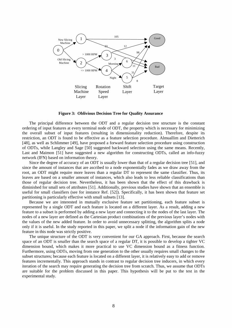
Figure 3 demonstrates a typical ODT with three input features: the slicing machine model used in the manufacturing process; the rotation speed of the slicing machine and the shift (i.e., when the item was manufactured); and the Boolean target feature representing whether that item passed the quality assurance test. The arcs that connect the hidden terminal nodes and the nodes of the target layer are labeled with the number of records that fit this path. For instance, the twelve items in the training set, which were produced using the old slicing machine that was set up to rotate at a speed greater than 1000 RPM, were classified as “good” items (i.e., passed the quality assurance test).
8
0
Bad
1
2
3
4
6
5
Good New Slicing Machine
Slicing Machine
Layer
Old Slicing Machine
Shift Layer
Night
Morning
Rotation Speed Layer
<= 1000 RPM
> 1000 RPM
Target Layer
105
23 12
3
8
31
98
11
Figure 3: Oblivious Decision Tree for Quality Assurance
The principal difference between the ODT and a regular decision tree structure is the constant
ordering of input features at every terminal node of ODT, the property which is necessary for minimizing the overall subset of input features (resulting in dimensionality reduction). Therefore, despite its restriction, an ODT is found to be effective as a feature selection procedure. Almuallim and Dietterich [48], as well as Schlimmer [49], have proposed a forward feature selection procedure using construction of ODTs, while Langley and Sage [50] suggested backward selection using the same means. Recently, Last and Maimon [51] have suggested a new algorithm for constructing ODTs, called an info-fuzzy network (IFN) based on information theory.
Since the degree of accuracy of an ODT is usually lower than that of a regular decision tree [51], and since the amount of instances that are ascribed to a node exponentially fades as we draw away from the root, an ODT might require more leaves than a regular DT to represent the same classifier. Thus, its leaves are based on a smaller amount of instances, which also leads to less reliable classifications than those of regular decision tree. Nevertheless, it has been shown that the effect of this drawback is diminished for small sets of attributes [51]. Additionally, previous studies have shown that an ensemble is useful for small classifiers (see for instance Ref. [52]). Specifically, it has been shown that feature set partitioning is particularly effective with small subsets [13].
Because we are interested in mutually exclusive feature set partitioning, each feature subset is represented by a single ODT and each feature is located on a different layer. As a result, adding a new feature to a subset is performed by adding a new layer and connecting it to the nodes of the last layer. The nodes of a new layer are defined as the Cartesian product combinations of the previous layer’s nodes with the values of the new added feature. In order to avoid unnecessary splitting, the algorithm splits a node only if it is useful. In the study reported in this paper, we split a node if the information gain of the new feature in this node was strictly positive.
The unique structure of the ODT is very convenient for our GA approach. First, because the search space of an ODT is smaller than the search space of a regular DT, it is possible to develop a tighter VC dimension bound, which makes it more practical to use VC dimension bound as a fitness function. Furthermore, using ODTs, moving from one generation to the other usually requires small changes to the subset structures; because each feature is located on a different layer, it is relatively easy to add or remove features incrementally. This approach stands in contrast to regular decision tree inducers, in which every iteration of the search may require generating the decision tree from scratch. Thus, we assume that ODTs are suitable for the problem discussed in this paper. This hypothesis will be put to the test in the experimental study.

9
2.7 Originality and contribution
The novel contributions of this paper include: • A new encoding schema specifically designed for feature set partitioning. The new encoding
eliminates the redundancy of existing encodings. Together with the new encoding, we also suggest a new crossover operator called "group-wise crossover" (GWC). The new encoding ensures the convergence of the genetic algorithm.
• The use of a structural risk measure to compute the fitness function. The new measure is much faster than the wrapper approach, which is frequently used in studies reported in the literature.
• A new caching mechanism to speed up the execution and avoid recreation of the same classifier.
• An examination of the hypothesis that ODTs are suitable for feature set partitioning. • A detailed experimental study encompassing benchmark data and synthetic data.
3. Problem Formulation In a typical classification problem, a training set of labelled examples is given. The training set can be described in a variety of languages, most frequently, as a collection of records that may contain duplicates. A vector of feature values describes each record. The notation A denotes the set of input features containing n features: },...,,...,{ 1 ni aaaA = -and y represents the class variable or the target
feature. Features (sometimes referred to as attributes) are typically one of two types: categorical (values are members of a given set), or numeric (values are real numbers). When the feature ia is categorical, it
is useful to denote its domain values by ( )idom a . In a similar way, },...,{)( )(1 ydomccydom = represents
the domain of the target feature. Numeric features have infinite cardinalities. The instance space (the set of all possible examples) is defined as a Cartesian product of all the input
feature domains: )(...)()( 21 nadomadomadomX ×××= . The universal instance space (or the labelled
instance space) U is defined as a Cartesian product of all input feature domains and the target feature domain, i.e., )(ydomXU ×= .The training set consists of a set of m records and is denoted as
1( , ,..., , )mS y y= < > < >1 mx x where X∈qx and )(ydomyq ∈ .
Usually, it is assumed that the training set records are generated randomly and independently according to some fixed and unknown joint probability distribution D over U. Note that this is a generalization of the deterministic case when a supervisor classifies a record using a function ( )y f= x .
The notation I represents a probabilistic inducer (i.e., an algorithm that generates classifiers that also provide estimates of the conditional probability of the target feature given the input features), and ( )I S represents a probabilistic classifier which was induced by activating the induction method I onto dataset
S. In this case it is possible to estimate the conditional probability ( )ˆ ( )I S jP y c= qx of an observation xq.
Note the addition of the “hat” - ^ - to the conditional probability estimation is used to distinguish it from the actual conditional probability. We denote the projection of an instance qx onto a subset of features G
as Gπ qx . Similarly the projection of a training set S onto G is denoted as GSπ .
The problem of partitioning an input feature set is to find the best partition such that, if a specific inducer is trained on each feature subset data, then the combination of the generated classifiers will have the highest possible degree of accuracy. Consequently the problem can be formally phrased as follows:
Given an inducer I, a combination method C, and a training set S with input feature set },...,,{ 21 naaaA = and target feature y from a distribution D over the labeled instance space, the goal
is to find an optimal partitioning 1{ ,... ..., }opt kZ G G Gω= of the input feature set A into ω mutually
exclusive subsets kG A⊆ that are not necessarily exhaustive. Optimality is defined in terms of

10
minimization of the generalization error of the induced classifiers ( ) ; 1,...,kG yI S kπ ω∪
= combined
using method C over the distribution D. In this paper we assume that I is any decision tree inducer and C is the naïve Bayes combination. In
the naïve Bayes combination, a classification of a new instance is based on the product of the conditional probability of the target feature, given the values of the input features in each subset. Mathematically it can be formulated as follows:
( )( )
( )( ) 1 ( )
ˆˆ( ) arg max ( )
ˆ ( )G y kk
j
I S j G
MAP I S jc dom y k I S j
P y cv P y c
P y c
ω π π∪
∈ =
== = ⋅
=∏ q
q
xx (1)
or:
( )( )1
1( ) ( )
ˆ
( ) arg maxˆ ( )
G y kk
j
I S j Gk
MAPc dom y I S j
P y cv
P y c
ω
π
ω
π∪
=−
∈
==
=
∏ q
q
xx . (2)
In the case of decision trees, ( )( )ˆ
G y kkI S j GP y cπ π
∪= qx can be estimated by using the appropriate
frequencies in the relevant leaf. It should be noted that the optimal partitioning structure is not necessarily unique. Furthermore it is not obligatory that all input features actually belong to one of the subsets. Consequently, the problem can be treated as an extension of the feature selection problem, i.e., finding the optimal partitioning of the form optZ 1{ }G= , as the non-relevant features are in fact NR=A-G1. Moreover,
when using a naïve Bayes for combining the classifiers as in this case, the naïve Bayes method can be treated as specific partitioning: Z 1 2{ , ,..., }nG G G= , where { }i iG a= .
Definition 1: Classification-Preservation Partitioning The partitioning 1{ ,..., ,..., }kZ G G Gω= is said to be classification-preservation if, for each instance in
the support of ( )P qx , the following is satisfied:
( ) ( )11
( ) ( )arg max arg max
( )
k
j j
j Gk
jc dom y c dom yj
P y cX P y c
P y c
ω
ω
π=
−∈ ∈
=∀ ∈ = =
=
∏q
xqxqx . (3)
Since the right term of the equation is optimal, it follows that classification-preservation partitioning is also optimal. The importance of finding classification-preservation partitioning is derived from the fact that in real problems with limited training sets it is easier to approximate probabilities with fewer dimensions.
The following four lemmas are presented in order to shed light on the suggested problem. This set of lemmas defines classification-preservation and demonstrates that conditional independence is not a necessary precondition. More specifically, these lemmas show that the naïve Bayes combination can be useful in various cases of separable functions even when the naïve assumption of conditional independence is not necessarily fulfilled. Furthermore because these lemmas provide the optimal partitioning structures, they can be used for evaluating the performance of the algorithms proposed in Section 4. The proofs of these lemmas are straightforward and appear in the appendix.

11
Lemma 1: Sufficient condition Let Z be a partitioning that satisfies the following conditions:
1. The subsets , 1,...,kG k ω= and the 1k kNR A Gω== −∪ are conditionally independent given
the target feature; 2. The NR set and the target feature are independent.
then Z is classification-preservation. Lemma 1 represents a sufficient condition for classification-preservation. It is important to note that it
does not represent a necessary condition, as illustrated in the following lemma: Lemma 2: The Read-Once DNF Case Let 1{ ,..., ,..., }l nA a a a= denote a group of n independent input binary features and let 1{ ,..., }Z G Gω=
denote a partitioning. If the target feature follows the function
1 1 2 2( , ) ( , ) ... ( , )i i iy f a i R f a i R f a i Rω ω= ∈ ∨ ∈ ∨ ∨ ∈ or
1 1 2 2( , ) ( , ) ... ( , )i i iy f a i R f a i R f a i Rω ω= ∈ ∧ ∈ ∧ ∧ ∈
where 1,...,f fω are Boolean functions and 1,...,R Rω are mutually exclusive, then Z is classification-
preservation. Lemma 3: The Additive Case Let 1{ ,..., ,..., }l nA a a a= be a group of n independent input binary features and let
1{ ,..., }Z G Gω= be a partitioning. If the target feature follows the function
),(2...),(2),(2 122
111
0ωω
ω RiafRiafRiafy iii ∈++∈⋅+∈⋅= −
where 1,...,f fω are Boolean functions and 1,...,R Rω are mutually exclusive, then Z is classification-
preservation.
Lemma 2 and Lemma 3 illustrate that, although the conditionally independence requirement is not fulfilled, it is still possible to find a classification-preservation partitioning. Lemma 4: The XOR Case Let 1{ ,..., ,..., }i nA a a a= be a group of n input binary features distributed uniformly. If the target feature
behaves as 1 2 ... ny a a a= ⊕ ⊕ ⊕ , then there is no partitioning beside { }Z A= , which is classification-
preservation. Lemma 4 shows that there are problems such that no classification-preservation partitioning can be
found, besides the obvious one.
The number of combinations into which n* input features may be decomposed exactly ω relevant subsets is:
( ) ( ) *
0
1( *, ) 1
!j n
j
Q n jj
ω ωω ω
ω =
= − −
∑ . (4)
Evidently the number combinations into which n* input features may be decomposed up to n* subsets is:
( ) ( )* *
*
1 1 0
1( *) ( *, ) 1
!
n nj n
j
C n Q n jj
ω
ω ω
ωω ω
ω= = =
= = − −
∑ ∑ ∑ . (5)
12
In the feature set partitioning problem defined above, it is possible that part of the input feature will not be used by the inducers (the irrelevant set). Thus, the total search space is then:
( ) ( )*
*
* 0 * 0 1 0
1( ) ( *) 1
* * !
n n nj n
n n j
n nT n C n j
n n j
ω
ω
ωω
ω= = = =
= = − −
∑ ∑ ∑ ∑ . (6)
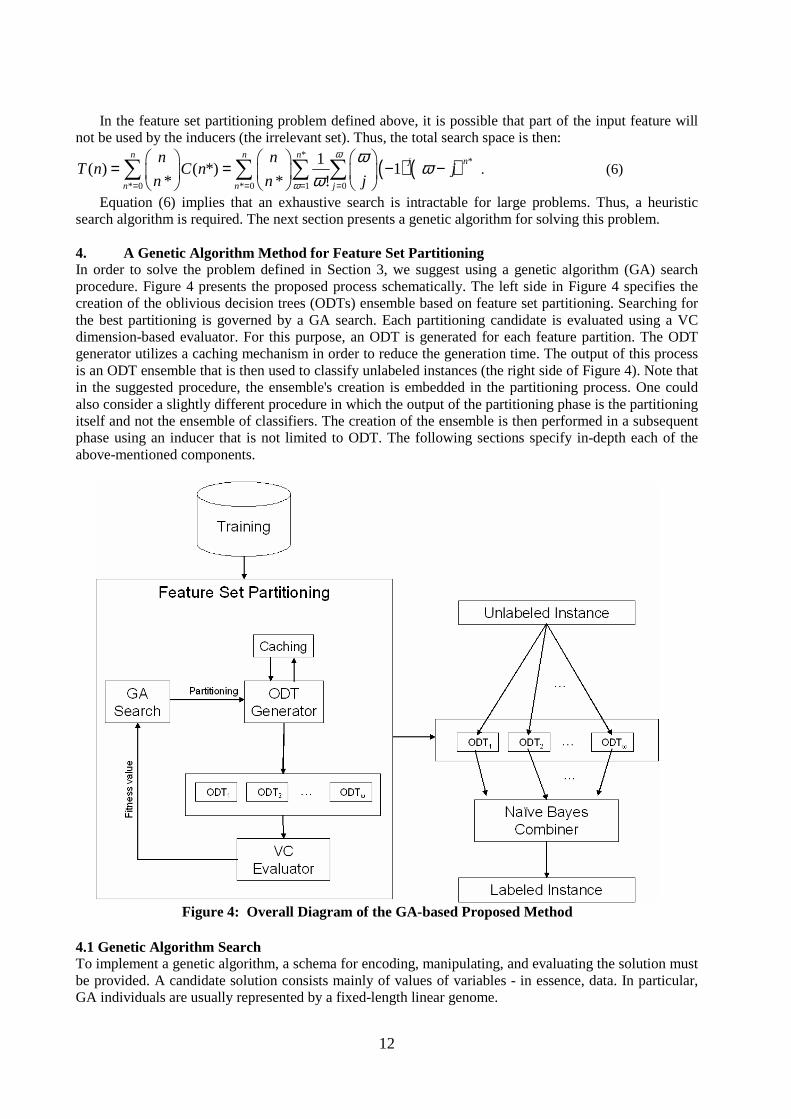
Equation (6) implies that an exhaustive search is intractable for large problems. Thus, a heuristic search algorithm is required. The next section presents a genetic algorithm for solving this problem. 4. A Genetic Algorithm Method for Feature Set Partitioning In order to solve the problem defined in Section 3, we suggest using a genetic algorithm (GA) search procedure. Figure 4 presents the proposed process schematically. The left side in Figure 4 specifies the creation of the oblivious decision trees (ODTs) ensemble based on feature set partitioning. Searching for the best partitioning is governed by a GA search. Each partitioning candidate is evaluated using a VC dimension-based evaluator. For this purpose, an ODT is generated for each feature partition. The ODT generator utilizes a caching mechanism in order to reduce the generation time. The output of this process is an ODT ensemble that is then used to classify unlabeled instances (the right side of Figure 4). Note that in the suggested procedure, the ensemble's creation is embedded in the partitioning process. One could also consider a slightly different procedure in which the output of the partitioning phase is the partitioning itself and not the ensemble of classifiers. The creation of the ensemble is then performed in a subsequent phase using an inducer that is not limited to ODT. The following sections specify in-depth each of the above-mentioned components.
Figure 4: Overall Diagram of the GA-based Proposed Method
4.1 Genetic Algorithm Search To implement a genetic algorithm, a schema for encoding, manipulating, and evaluating the solution must be provided. A candidate solution consists mainly of values of variables - in essence, data. In particular, GA individuals are usually represented by a fixed-length linear genome.

13
A straightforward individual representation for feature set partitioning consists simply of a string of n integers. Recall that n is the number of features. The i-th integer, i=1,…, n, can take the value 0,…,n, indicating to which subset (if any) the i-th feature belongs. A value of 0 indicates that the corresponding feature is not selected and is filtered out. For instance, in a 10-feature dataset, the individual '1 0 2 0 1 3 3 2 0 1' represents a candidate solution where the 1st, 5th and 10th features are located in the first subset. The 3rd and 8th are located in the second subset. The 6th and the 7th are located in the third group. All other features are filtered out. This individual representation is simple, and a traditional one-point crossover operator can easily be applied. As for the mutation operator, according to a certain probability (Pmut), each integer is changed from its current value to a different valid value.
The last representation has redundancy, i.e., the same solution can be represented in several ways. For instance, the illustrated solution '1 0 2 0 1 3 3 2 0 1' can be also represented as '3 0 1 0 3 2 2 1 0 3'. Moreover, similar solutions can be represented in quite different ways. This property can lead to situations in which the offspring are dissimilar to their parents. For example, if we perform the one-point crossover operator on the two equal solutions above -- '1 0 2 0 1 3 3 2 0 1' and '3 0 1 0 3 2 2 1 0 3' -- we may obtain the following descendant solution '1 0 2 0 3 5 5 1 0 3'. Because the two parents are equal, we expect that the descendant (before mutation) should also be equal. However, this is not the case here and the descendant represents quite a different solution. Although the above case is rare, it still illustrates the problematic character of the above representation. Besides not being compact, the above encoding may result in a slow convergence of the genetic algorithm. We begin by defining a measure called partitioning structural distance. This measure can be used to determine the distance of two partitioning structures as follows:
Definition 2: Partitioning Structural Distance (Revised Rand index):
∑ ∑−
= += −⋅⋅
=1
1 1
2121
)1(
),,,(2),(
n
i
n
ij
ji
nn
ZZaaZZ
ηδ
(7)
where 1 2( , , , )i ja a Z Zη is a binary function that returns the value "0" if the features ,i ja a belong to the
same subset in both partitioning structures 1 2,Z Z or if ,i ja a belong to different subsets in both
partitioning structures. In all other cases the function returns the value "1".
∈∈∈∈≠≠∃∈∈∃
∉∉∈∈
∈∈∉∉
∉∉∉∉
=
====
====
====
otherwise
RjRiRjRikkkk
RjiRjikk
RjRjandRiRi
RjRjandRiRi
RjRjandRiRi
ZZaa
kkkk
kk
kk
kk
kk
kk
kk
kk
kk
kk
kk
kk
kk
kk
ji
1
,;,;,0
,,,;,0
;;0
;;0
;;0
),,,(
22112,21,22,11,1
2121
1
2
1
1
1
2
1
1
1
2
1
1
1
2
1
1
1
2
1
1
1
2
1
1
21
2,21,22,11,1
21
2
2
2
1
1
1
2
2
2
1
1
1
2
2
2
1
1
1
2
2
2
1
1
1
2
2
2
1
1
1
2
2
2
1
1
1
∪∪∪∪
∪∪∪∪
∪∪∪∪
ωωωω
ωωωω
ωωωω
η (8)
For example, given that },,,,,{ 654321 aaaaaaA = , { }14 2 5 3{ , };{ , }Z a a a a= and
{ }21 3 5 2 4{ , , };{ , }Z a a a a a= then:

14
15
5)000000000011111(
30
2)),,,(
),,,(),,,(),,,(),,,(
),,,(),,,(),,,(),,,(
),,,(),,,(),,,(),,,(
),,,(),,,((65
2
)1(
),,,(2),(
2165
2164
2154
2163
2153
2143
2162
2152
2142
2132
2161
2151
2141
2131
2121
1
1 1
2121
=++++++++++++++=+
++++
++++
++++
+⋅
=−⋅
⋅=∑ ∑
−
= +=
ZZaa
ZZaaZZaaZZaaZZaa
ZZaaZZaaZZaaZZaa
ZZaaZZaaZZaaZZaa
ZZaaZZaann
ZZaaZZ
n
i
n
ij
ji
η
ηηηηηηηη
ηηηη
ηηη
δ
.
By using an adjacency matrix-like encoding, one can represent any partitioning structure as n x n matrix B in which Bi, j = 1 if features ai and aj are located in the same group. Additionally Bi, j = 1 if features ai and aj are both filtered out. In any other case Bi, j=0. The values on the diagonal indicate whether each feature is included in one of the subsets (1) or not (-1). For example, Table 1 illustrates the
representation of { }14 2 5 3{ , };{ , }Z a a a a= given that },,,,,{ 654321 aaaaaaA = . Note that because the
above matrix is always symmetric, we can specify only the upper triangle.
Table 1: Illustration of adjacency matrix like encoding a1 a2 a3 a4 a5 a6 a1 -1 0 0 0 0 -1 a2 0 1 0 1 0 0 a3 0 0 1 0 1 0 a4 0 1 0 1 0 0 a5 0 0 1 0 1 0 a6 -1 0 0 0 0 -1
Definition 3: Encoding Matrix B is said to be well-defined if:
1. Commutative: , ,; i j j ii j B B∀ ≠ =
2. Transitive: , , ,; 0 0 0i j i k j ki j k if B and B then B∀ ≠ ≠ ≠ ≠ ≠
3. Sign Property: , , ,; 0i j i j i ii j if B then B B∀ ≠ ≠ = .
We now suggest a new crossover operator called "group-wise crossover" (GWC). In this operator, we
select one anchor subset from the subsets that define the first parent partitioning and one anchor subset from the subsets that define the second parent partitioning (the selected subset can also be the filtered-out subset). The anchor subsets are used as is, without any addition or diminution of features.
The first offspring is created by copying the columns and rows of the features that belong to the first selected anchor subset from the first parent. All remaining elements in B are filled in with the corresponding values that are obtained from the second parent. The second offspring is similarly created, using the second anchor subset by copying the appropriate columns and the rows from the second parent. The remaining elements are filled in with the corresponding values from the first parent.
Example: Assume that two partitioning structures { }14 2 5 3{ , };{ , }Z a a a a= and
{ }22 6 1 4 3 5{ , };{ , , }{ }Z a a a a a a= are given over the feature set },,,,,{ 654321 aaaaaaA = . In order to use
a GWC operator, two anchor subsets are selected, one from each partitioning, 2 4{ , }a a from Z1 and

15
1 4 3{ , , }a a a from Z2. Table 2 illustrates representations of the Z1 and Z2 and their offspring Z3 and Z4. Z3 is
obtained by keeping the group 2 4{ , }a a while the remaining elements are copied from Z2. Z4 is obtained
by keeping the group 1 4 3{ , , }a a a while the remaining elements are copied from Z1. Thus,
{ }32 4 1 3 5 6{ , };{ , };{ };{ }Z a a a a a a= and { }4
1 4 3 5 2{ , , };{ };{ }Z a a a a a= . The highlighted elements
indicate the selected group that was copied into the offspring.
Table 2: Illustration of GWC operator Z1 Z2
a1 a2 a3 a4 a5 a6 a1 a2 a3 a4 a5 a6 a1 -1 0 0 0 0 -1 a1 1 0 1 1 0 0 a2 0 1 0 1 0 0 a2 0 1 0 0 0 1 a3 0 0 1 0 1 0 a3 1 0 1 1 0 0 a4 0 1 0 1 0 0 a4 1 0 1 1 0 0 a5 0 0 1 0 1 0 a5 0 0 0 0 1 0 a6 -1 0 0 0 0 -1 a6 0 1 0 0 0 1
Z3 Z4
a1 a2 a3 a4 a5 a6 a1 a2 a3 a4 a5 a6 a1 1 0 1 0 0 0 a1 1 0 1 1 0 0 a2 0 1 0 1 0 0 a2 0 1 0 0 0 0 a3 1 0 1 0 0 0 a3 1 0 1 1 0 0 a4 0 1 0 1 0 0 a4 1 0 1 1 0 0 a5 0 0 0 0 1 0 a5 0 0 0 0 1 0 a6 0 0 0 0 0 1 a6 0 0 0 0 0 -1
The following set of lemmas shows that the well-defined property of an adjacency matrix is preserved under a group-wise crossover operator.
Lemma 5: Structural Distance Measure Properties
The structural distance measure has the following properties:
1. Symmetry: ),(),( 1221 ZZZZ δδ =
2. Positivity: 0),( 21 =ZZδ Iff 21 ZZ =
3. Triangular Inequality: ),( 21 ZZδ ≤ ),( 31 ZZδ + ),( 32 ZZδ .
Lemma 6: A projection of a well-defined encoding matrix is a well-defined encoding matrix.
Lemma 7: Using a GWC operator on two well-defined encoding matrices generates a new well-defined encoding matrix
Lemma 8: Operator GWC creates two offspring with an inter-distance that is not greater than the inter-distance of their parents.

16
Lemma 8 indicates that the GWC operator together with the proposed encoding does not slow down the convergence of the genetic algorithm. Together with the selection process that prefers solutions with higher fitness values, one can ensure that the algorithm converges.
As to the mutation operator, according to a certain probability (Pmut) each feature can be cut off from its original group to join another randomly selected group. 4.2 Fitness Function In each iteration, we have to create a new population from the current generation. The selection operation determines which parent chromosomes participate in producing offspring for the next generation. Usually, members are selected for mating with a selection probability proportional to their fitness values. The most common way to implement this method is to set the selection probability pi equal to:
ii
jj
fpf
=∑
. (9)
For a classification problem, the fitness value fi of the i-th member can be the generalized accuracy.
Note that using training accuracy as is does not suffice to evaluate classifiers due to the over-fitting phenomena.
The most straightforward way to estimate generalization error is to use the wrapper procedure. In this approach the partitioning structure is evaluated by repeatedly sampling the training set and measuring the accuracy of the inducers obtained for this partitioning on an unused portion of the training set. This is the most common approach for evaluating the fitness function in feature selections problems. However, as stated in Section 2, the fact that the wrapper procedure repeatedly executes the inducer is considered a major drawback. According to the VC theory, the bound on the generalization error of hypothesis space H with finite VC-Dimension d is given by:
md
md
ShDh 4ln)1
2(ln
),(ˆ),(
δ
εε−+⋅
≤− 0>∀
∈∀δ
Hh
(10) with probability of 1 δ− where ˆ( , )h Sε represents the training error of classifier h measured on training
set S of cardinality m, and ( , )h Dε represents the generalization error of the classifier h over the
distribution D. Note that in this case fi = 1- ( , )ih Dε .
In order to use the bound (Equation 10), one needs to measure the VC dimension. The VC dimension for a set of indicator functions is defined as the maximum number of data points that can be shattered by the set of admissible functions. By definition, a set of m points is shattered by a concept class if there are concepts (functions) in the class that split the points into two classes in all of the 2m possible ways. The VC dimension, which might be difficult to compute accurately, depends on the induction algorithm.
As stated before, using an ODT may be attractive in this case since it adds features to a classifier in an incremental manner. Due to the fact that ODTs can be considered as restricted decision trees, any generalization error bound that has been developed for decision trees in studies reported in the literature can be used in this case as well. However, there are several reasons for developing a specific bound. First, by utilizing the fact that the oblivious structure is more restricted, it might be possible to develop a tighter bound. Second, it is necessary to extend the bound for several oblivious trees combined using the naïve Bayes combination.
The following theorem introduces an upper and lower bound of the VC dimension that was recently used by the DOG algorithm. The hypothesis class of multiple mutually exclusive ODTs can be
characterized by two vectors and one scalar: 1( ,..., )L l lω=�
, 1( ,..., )T t tω=�
and n, where lk is the
17
numbers of layers (not including the root and target layers) in the tree k, tk is the number of terminal nodes in the tree k, and n is the number of input features.
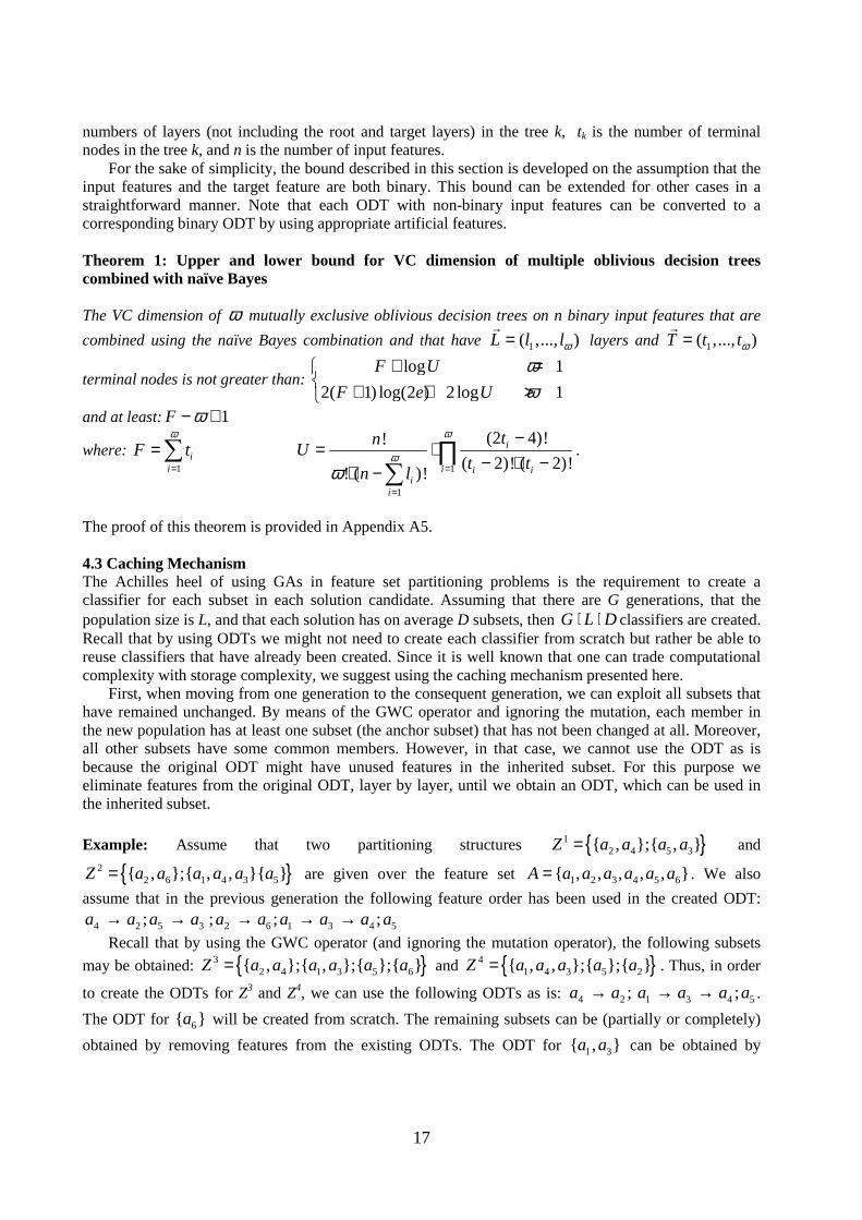
For the sake of simplicity, the bound described in this section is developed on the assumption that the input features and the target feature are both binary. This bound can be extended for other cases in a straightforward manner. Note that each ODT with non-binary input features can be converted to a corresponding binary ODT by using appropriate artificial features. Theorem 1: Upper and lower bound for VC dimension of multiple oblivious decision trees combined with naïve Bayes The VC dimension of ω mutually exclusive oblivious decision trees on n binary input features that are
combined using the naïve Bayes combination and that have 1( ,..., )L l lω=�
layers and 1( ,..., )T t tω=�
terminal nodes is not greater than: log 1
2( 1) log(2 ) 2 log 1
F U
F e U
ωω
+ = + + >
and at least: 1F ω− +
where: 1
ii
F tω
=
=∑ 1
1
(2 4)!!
( 2)! ( 2)!! ( )!
i
i i ii
i
tnU
t tn l
ω
ω
ω =
=
−= ⋅
− ⋅ −⋅ −∏
∑.
The proof of this theorem is provided in Appendix A5. 4.3 Caching Mechanism The Achilles heel of using GAs in feature set partitioning problems is the requirement to create a classifier for each subset in each solution candidate. Assuming that there are G generations, that the population size is L, and that each solution has on average D subsets, then DLG ⋅⋅ classifiers are created. Recall that by using ODTs we might not need to create each classifier from scratch but rather be able to reuse classifiers that have already been created. Since it is well known that one can trade computational complexity with storage complexity, we suggest using the caching mechanism presented here.
First, when moving from one generation to the consequent generation, we can exploit all subsets that have remained unchanged. By means of the GWC operator and ignoring the mutation, each member in the new population has at least one subset (the anchor subset) that has not been changed at all. Moreover, all other subsets have some common members. However, in that case, we cannot use the ODT as is because the original ODT might have unused features in the inherited subset. For this purpose we eliminate features from the original ODT, layer by layer, until we obtain an ODT, which can be used in the inherited subset.
Example: Assume that two partitioning structures { }12 4 5 3{ , };{ , }Z a a a a= and
{ }22 6 1 4 3 5{ , };{ , , }{ }Z a a a a a a= are given over the feature set },,,,,{ 654321 aaaaaaA = . We also
assume that in the previous generation the following feature order has been used in the created ODT:
4 2 5 3;a a a a→ → 2 6 1 3 4 5; ; ;a a a a a a→ → →
Recall that by using the GWC operator (and ignoring the mutation operator), the following subsets
may be obtained: { }32 4 1 3 5 6{ , };{ , };{ };{ }Z a a a a a a= and { }4
1 4 3 5 2{ , , };{ };{ }Z a a a a a= . Thus, in order
to create the ODTs for Z3 and Z4, we can use the following ODTs as is: 4 2;a a→ 1 3 4 5;a a a a→ → .
The ODT for 6{ }a will be created from scratch. The remaining subsets can be (partially or completely)
obtained by removing features from the existing ODTs. The ODT for 1 3{ , }a a can be obtained by

18
removing feature 4a from 1 3 4a a a→ → . This removal is possible since 4a is located last. The ODT
for 2{ }a can be obtained by removing feature 6a from 2 6a a→ .
In addition to the ODTs of the previous generations, we can use the existing ODTs in a different subset of the current generation. While generating an ODT, we check at the end of each iteration (i.e., after adding a new feature to the ODT) whether there is another solution in the current generation that also groups these features together in the same subset. If this is the case, we store the current ODT in the cache for future use. Later, when the time has come to generate the ODT for the solution with the common subset, instead of creating the tree from scratch we make use of the tree that was stored in the caching mechanism. For example, we are given in the first generation the following members:
{ }11 4 5 6 2 3 8 10 7 9{ , , , }; { , , , }; { , }Z a a a a a a a a a a=
{ }21 5 6 8 2 3 4 10 7 9{ , , , }; { , , , }; { , }Z a a a a a a a a a a=
{ }31 3 4 5 6 2 8 10 7 9{ , , , , }; { , , }; { , }Z a a a a a a a a a a=
Assuming that we are evaluating the members one by one according to the above order, and that while creating the tree for the first subset in the first solution we get an ODT with the following order
5 1 6 a a a→ → , then we might want to store this ODT in the caching mechanism, and use it also for
members 2 and 3. It should be noted that utilizing this caching mechanism reduces the search space, because it dictates
the order in which the features are located in the ODT. For instance, in the last example, the first tree of solution 2 could have the following structure: 8 1 5 6a a a a → → → . However, by using the ODT
5 1 6 a a a→ → that was stored in the cache, we a priori ignore this structure. In order to solve this
dilemma, we decide not to store small ODTs (in this paper fewer than 3 features). In such cases the saving in computational cost is not worth the loss in generalization capability.
Obviously, it is desirable to store the longest common subset in the cache. Thus, in each iteration we check if the current ODT can still be used by the same number of solutions. If this is the case, the current ODT will replace the older one.
4.4 Classification of an Unlabeled Instance After multiple ODTs have been created, the following steps may be performed to classify an unlabeled instance:
A. For each tree: 1. Locate the appropriate leaf for the unseen instance. For every instance there
is exactly one path from the root to the relevant leaf. The relevant leaf is chosen by navigating from the root of the tree down to a leaf, according to the outcome of the decision tests along the path.
2. Extract the frequency vector. The frequency vector has an entry for every possible class value. The value in a certain entry is calculated according to the number of training instances that have been navigated to the selected leaf and have been labeled with that class.
3. Transform the frequency vector to a probability vector according to Laplace's law of succession, as described in Section 2.
B. Combine the probability vectors using the naïve Bayes combination. C. Select the class that maximizes the naïve Bayes combination. In the case of a tie, we
select the class with the highest a-priori probability.
5. Experimental Study In order to illustrate the potential of the feature set partitioning approach in classification problems and to evaluate the performance of the proposed genetic algorithm, a comparative experiment was conducted on benchmark datasets. The following subsections describe the experimental set-up and the results obtained.
19
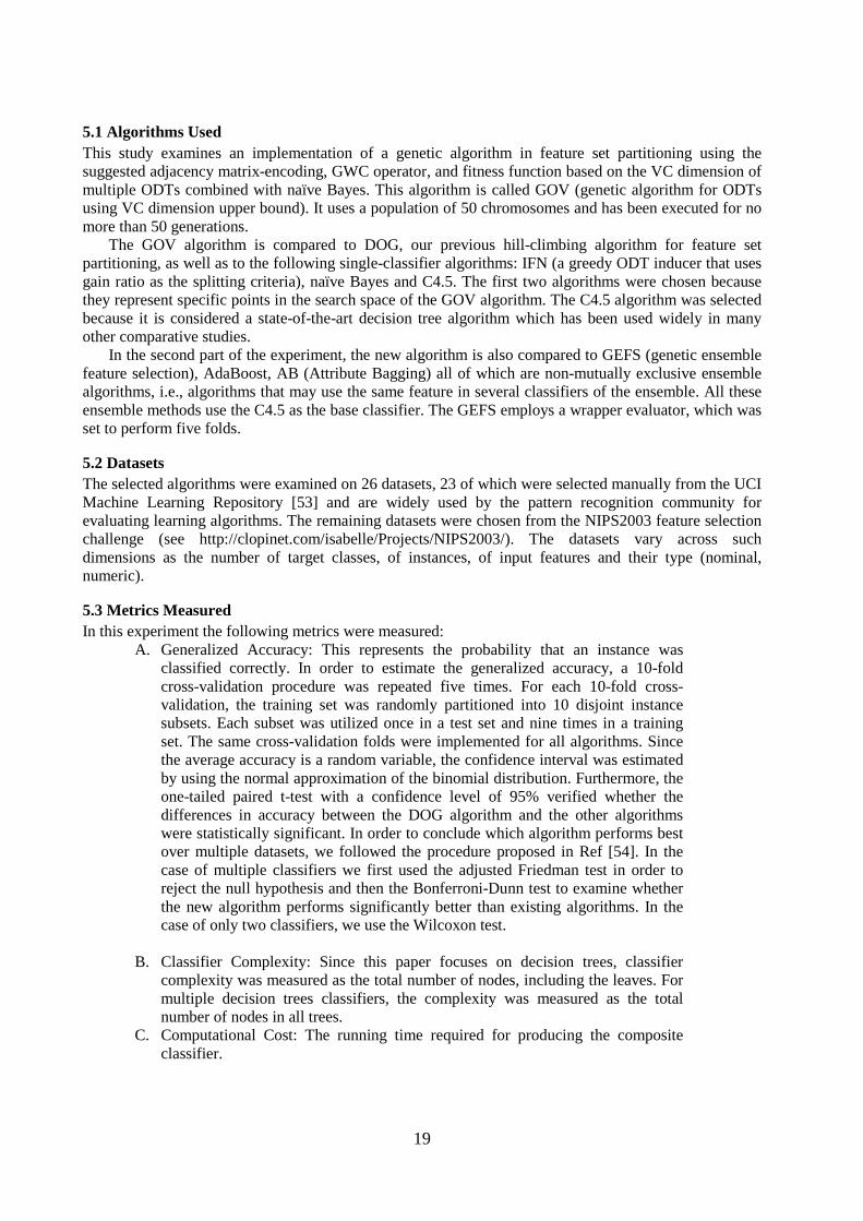
5.1 Algorithms Used This study examines an implementation of a genetic algorithm in feature set partitioning using the suggested adjacency matrix-encoding, GWC operator, and fitness function based on the VC dimension of multiple ODTs combined with naïve Bayes. This algorithm is called GOV (genetic algorithm for ODTs using VC dimension upper bound). It uses a population of 50 chromosomes and has been executed for no more than 50 generations.
The GOV algorithm is compared to DOG, our previous hill-climbing algorithm for feature set partitioning, as well as to the following single-classifier algorithms: IFN (a greedy ODT inducer that uses gain ratio as the splitting criteria), naïve Bayes and C4.5. The first two algorithms were chosen because they represent specific points in the search space of the GOV algorithm. The C4.5 algorithm was selected because it is considered a state-of-the-art decision tree algorithm which has been used widely in many other comparative studies.
In the second part of the experiment, the new algorithm is also compared to GEFS (genetic ensemble feature selection), AdaBoost, AB (Attribute Bagging) all of which are non-mutually exclusive ensemble algorithms, i.e., algorithms that may use the same feature in several classifiers of the ensemble. All these ensemble methods use the C4.5 as the base classifier. The GEFS employs a wrapper evaluator, which was set to perform five folds.
5.2 Datasets The selected algorithms were examined on 26 datasets, 23 of which were selected manually from the UCI Machine Learning Repository [53] and are widely used by the pattern recognition community for evaluating learning algorithms. The remaining datasets were chosen from the NIPS2003 feature selection challenge (see http://clopinet.com/isabelle/Projects/NIPS2003/). The datasets vary across such dimensions as the number of target classes, of instances, of input features and their type (nominal, numeric).
5.3 Metrics Measured In this experiment the following metrics were measured:
A. Generalized Accuracy: This represents the probability that an instance was classified correctly. In order to estimate the generalized accuracy, a 10-fold cross-validation procedure was repeated five times. For each 10-fold cross- validation, the training set was randomly partitioned into 10 disjoint instance subsets. Each subset was utilized once in a test set and nine times in a training set. The same cross-validation folds were implemented for all algorithms. Since the average accuracy is a random variable, the confidence interval was estimated by using the normal approximation of the binomial distribution. Furthermore, the one-tailed paired t-test with a confidence level of 95% verified whether the differences in accuracy between the DOG algorithm and the other algorithms were statistically significant. In order to conclude which algorithm performs best over multiple datasets, we followed the procedure proposed in Ref [54]. In the case of multiple classifiers we first used the adjusted Friedman test in order to reject the null hypothesis and then the Bonferroni-Dunn test to examine whether the new algorithm performs significantly better than existing algorithms. In the case of only two classifiers, we use the Wilcoxon test.
B. Classifier Complexity: Since this paper focuses on decision trees, classifier
complexity was measured as the total number of nodes, including the leaves. For multiple decision trees classifiers, the complexity was measured as the total number of nodes in all trees.
C. Computational Cost: The running time required for producing the composite classifier.

20
The following additional metrics were measured in order to characterize the partitioning structures obtained by the GOV algorithm:
A. Number of subsets B. Average number of features in a single subset.
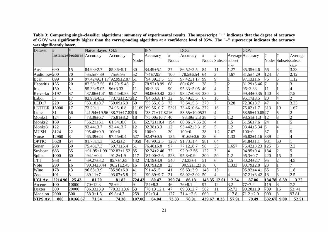
5.4 Comparing Single-Classifier Algorithms Table 3 presents the results obtained by averaging five standard 10-fold cross-validation experiments. The results indicate that there is no significant case where either naïve Bayes or IFN was more accurate than GOV. On the other hand, GOV was significantly more accurate than naïve Bayes and IFN in 16 databases and 14 databases, respectively. Moreover, GOV was significantly more accurate than C4.5 in 13 databases, and less accurate in only two databases. GOV's classifier complexity (total number of nodes) was comparable to the complexity the C4.5 algorithm obtained in most of the cases.
The results of the experimental study are encouraging. On the datasets obtained from the UCI repository, the GOV outperformed naïve Bayes mostly when the data were large in size or had a small number of features. For moderate dimensionality (from 50 features up to 500), the performance of naïve Bayes was not necessarily inferior. More specifically, regarding the datasets OPTIC, SONAR, SPI, AUDIOLOGY, LUNG-CANCER, the superiority of GOV over naïve Bayes was statistically significant only in three features (SPI, AUDIOLOGY, LUNG-CANCER). However, for high dimensionality datasets (having at least 500 features), GOV significantly outperforms naïve Bayes in all cases.
The null-hypothesis, that all classifiers perform the same and the observed differences are merely random, was rejected using the adjusted Friedman test. We proceeded with the Bonferroni-Dunn test and found that GOV statistically outperforms naïve Bayes and IFN with a 95% confidence level. Using Hochberg’s step-up procedure, we found that GOV statistically outperforms C4.5 with a confidence level of 90%.
Analysis of the number of features in each subset shows that the GOV algorithm tends to build small subsets. Moreover, there are two cases (OPTIC and MONKS3) in which the GOV algorithm used only one feature in each tree. In these cases the classifiers that were built are equivalent to naïve Bayes. This suggests that in some cases GOV acts as a feature selection procedure for naïve Bayes.
A comparison of the accuracy of GOV and DOG indicated that in most cases GOV obtained better results. This observation is not surprising, considering the fact that GOV performs a more intensive search than DOG. A comparison of the mean number of subsets obtained by DOG (11.58) and that obtained by GOV (6.7) indicates that DOG tends to have more subsets. Moreover, in 16 datasets out of 26 DOG incorporated more features than GOV. However, for high dimensionality datasets (having at least 500 features), GOV significantly used more features than DOG.
5.5 Comparing to Ensemble Algorithms Since the accuracy and the classifier complexity are affected by the ensemble size (number of classifiers), we examined various ensemble sizes. Following the empirical results for asymptotic convergence of ensembles [6], the ensemble sizes created using the GEFS algorithm included up to 15 classifiers. Similarly, the ensemble size created with the AdaBoost included up to 25 classifiers. Table 4 presents the results obtained based on a 10-fold cross-validation procedure which was repeated five times.
21
Table 3: Comparing single-classifier algorithms: summary of experimental results. The superscript "+" indicates that the degree of accuracy of GOV was significantly higher than the corresponding algorithm at a confidence level of 95%. The "–" superscript indicates the accuracy was significantly lower.
Naïve Bayes C4.5 IFN DOG GOV Dataset # Instances
# Features Accuracy Accuracy #
Nodes Accuracy #
Nodes Accuracy #
Nodes # Subsets
Average subset size
Accuracy # Nodes
# Subsets
Average subset size
Aust 690 15 84.93±2.7 85.36±5.1 30 84.49±5.1 27 86.52±2.5 84 11 1.27 85.35±4.6 56 3 3.33 Audiology 200 70 +65.5±7.39 +75±6.95 52 +74±7.95 100 +78.5±6.54 64 3 4.67 81.5±4.29 124 7 2.12 Bcan 699 10 97.4249±1.17 +92.99±2.87 61 +94.39±3.5 55 97.42±1.17 99 9 1 97.13±1.6 76 5 1.12 Hepatitis 155 20 82.58±7.56 81.29±5.46 7 78.97±8.99 68 80±6.89 38 2 2 81.29±5.46 7 1 3 Iris 150 5 95.33±5.05 96±3.33 11 96±3.33 90 95.33±5.05 40 4 1 96±3.33 11 1 4 Kr-vs-kp 3197 37 +87.86±1.41 99.44±0.55 87 98.06±0.42 220 98.47±0.63 330 2 7 99.44±0.35 140 3 7.5 Labor 57 17 92.98±4.52 +73.72±12.72 12 +84.63±8.14 32 96.49±5.5 67 16 1 95.17±3.5 20 4 2 LED17 220 25 +63.18±8.7 +59.09±6.9 69 +55.55±6.3 73 73.64±5.5 370 7 3.28 72.36±3.7 47 4 3.33 LETTER 15000 17 73.29±1 74.96±0.8 11169 +69.56±0.7 5321 73.46±0.64 272 16 1 75.02±1.7 313 10 1.67 Lung 31 56 +41.94±19.96 +38.71±17.82 16 +38.71±17.8216 53.55±10.0527 4 2 53.55±10.0527 5 2 Monks1 124 6 +73.39±6.7 +75.81±8.2 18 +75.00±10.7 40 98.39± 2.3 28 5 1.2 98.51± 1.3 12 3 2 Monks2 169 6 +56.21±6.1 61.54±8.6 31 62.72±10.4 194 60.36 ±7.55 30 4 1.5 61.56±7.6 24 1 5 Monks3 122 6 93.44±3.7 93.44±3.7 12 92.38±3.3 12 93.442±3.3 19 5 1.2 93.44±5.34 6 4 1 MUSH 8124 22 +95.48±0.9 100±0 28 100±0 30 100±0 28 1.2 7.67 100±0 37 1 5 Nurse 12960 8 +65.39±24 97.45±0.4 527 92.47±0.5 135 +91.65±0.6 38 6 1.33 96.82±1.16 339 2 4 OPTIC 5628 64 91.73±1.3 +62.42±2 4059 +48.90±2.5 1257 91.73±1.4 981 64 1 91.84±1.1 981 60 1 Sonar 208 60 75.48±7.3 +69.71±5.4 51 76.48±6.8 97 77.12±8.7 98 35 1.657 76.42±3.23 125 5 2.2 Soybean 683 35 +91.95±1.99 +92.83±1.52 85 92.24±2.46 72 92.9±2.56 122 3 4 94.95±0.4 134 2 5 Splice 1000 60 +94.1±0.4 +91.2±1.9 117 +87.00±2.6 523 95.8±0.9 300 50 1.2 96.3±0.7 420 15 3 TTT 958 9 +69.27±3.2 -85.7±1.65 142 73.19±3.9 540 +73.33±4 51 6 2.5 80.24±2.7 95 2 4.5 Vote 290 16 +90.34±3.44 -96.21±2.45 16 93.79±2.8 23 +90.52±1.23 18 6 1.333 93.79±2.8 23 1 7 Wine 178 13 96.63±3.9 +85.96±6.9 41 +91.45±5 41 96.63±3.9 143 13 1 95.92±4.41 65 5 1.8 Zoo 101 8 +89.11±7 +93.07±5.8 21 +90.89±9.7 21 98.02±3.02 50 4 4 97.21±3.42 18 3 2.5 UCI Av. 2214.96 25.43 81.20 81.82 724.43 80.47 390.74 86.13 143.35 12.01 2.34 87.06 134.78 6.39 3.22 Arcene 100 10000 +70±12.3 75 ±9.2 9 +54±8.3 46 76±8.1 97 12 3.2 77±7.2 119 8 7.2 Dexter 300 20000 +86.33±3.9 +78.33 ±3.6 53 +76.13 ±2.1 47 89.33±2.7 562 11 52.72 90.28±1.9 789 16 52. 41 Madelon 2000 500 +58.3±1.5 69.8±4.7 259 +62±3.4 127 71.4 ±2.6 660 2 117.8 71.2 ±2.9 990 3 97.81 NIPS Av. 800 10166.67 71.54 74.38 107.00 64.04 73.33 78.91 439.67 8.33 57.91 79.49 632.67 9.00 52.51

22
Table 4: Comparing ensemble algorithms: summary of experimental results for . The superscript "+" indicates that the degree of accuracy of GOV was significantly higher than the corresponding algorithm at a confidence level of 95%. The "–" superscript indicates the accuracy was significantly lower.
GEFS Adaboost AB GOV Dataset Accuracy # Nodes Ensembl
e Size Accuracy #
Nodes Ensemble Size
Accuracy # Nodes
Ensemble Size
Accuracy # Nodes # Subsets Average subset size
Aust 86.96±2.1 517.2 10 85.36±3.6 30 1 86.81±2.3 9 2 85.35±4.6 56 3 3.33 Audiology 81.1±7.29 562.7 12 83.5±4.25 471.2 8 +76±6.9 525 10 81.5±4.29 124 7 2.12 Bcan +94.66±2.17 822 14 96.71±2.7 1793 19 +93.4±2.8 117 3 97.13±1.6 76 5 1.12 Hepatitis 83.92±5.41 91.4 6 81.29±5.46 7 1 81.3± 5.8 7 1 81.29±5.46 7 1 3 Iris 97.11±2.27 77.1 8 96±3.33 11 1 95.3 ± 5.9 92 11 96±3.33 11 1 4 Kr-vs-kp +98.31±0.79 567.2 13 99.69±0.59 421 5 99.4 ±0.4 592 23 99.44±0.35 140 3 7.5 Labor +91.22±10.12 67.2 8 -100±0 59 5 +89.7±12.7 67 9 95.17±3.5 20 4 2 LED17 66.73±5.2 611.5 11 65.91±4.2 365.8 5 +60.4±3.7 716 10 72.36±3.7 47 4 3.33 LETTER -81.69±1.4 1065.2 15 -87.72±2.3 24031 20 -92.13±1.7 1923 19 75.02±1.7 313 10 1.67 Lung +48.22±10.82 99.9 10 -57.5±12.8 32.8 3 +46.9±14.1 142 10 53.55±10.0 27 5 2 Monks1 +81.36±8.2 51.6 2 97.56±7.4 307.1 18 +92.74± 15 3 98.51± 1.3 12 3 2 Monks2 61.22±9.1 474.8 14 62.76±6.4 371.5 13 62.13±2 8 4 61.56±7.6 24 1 5 Monks3 +89.1±2.6 44.7 3 93.73±2.3 297.1 14 93.4±5.3 24 2 93.44±5.34 6 4 1 MUSH 100±0 90.4 3 100±0 30 1 100±0 328 10 100±0 37 1 5 Nurse 96.64±1.2 5495.9 12 -98.2±1.5 6069 19 -97.4±0.31 55 9 96.82±1.16 339 2 4 OPTIC +78.22±1.5 45111 5 +87.24±2.1 73838 20 +60.53±1.2 40702 11 91.84±1.1 981 60 1 Sonar 74.95±1.6 502 3 -79.24±6.7 994 16 71.1± 8.1 107 2 76.42±3.23 125 5 2.2 Soybean 94.44±2.51 1257.6 13 93.47±2.51 1271 15 91.8±1.7 967 10 94.95±0.4 134 2 5 Splice +92.1±2.1 1042.6 9 +93.7±4.6 2331 19 +94.5±1.7 1170 19 96.3±0.7 420 15 3 TTT -94.58±0.59 1959.2 15 -97.29±3.9 1906 15 -88±1.67 1721 12 80.24±2.7 95 2 4.5 Vote -96.55±3.21 156.2 12 -96.21±2.3 16 1 -95.86±2.5 76 10 93.79±2.8 23 1 7 Wine -89.87±4.1 256 5 95.56±6.1 513 11 90.44±3.2 391 14 95.92±4.41 65 5 1.8 Zoo 94.09±2.4 141.6 9 -100±0 110 7 +92.0±4.52 127 8 97.21±3.42 18 3 2.5 UCI Av. 85.78 2655.00 9.22 89.07 14415 10.30 84.83 2168 9.2 87.06 134.78 6.39 3.22
Arcene 76 ±8.4 161 16 78±5.2 467 10 75±9.08 149 11 77±7.2 119 8 7.2 Dexter +80.12 ±1.9 478 9 +81.13 ±3.1 391 7 87±2.4 1720 25 90.28±1.9 789 16 52. 41 Madelon 70.9±5.1 2725 10 +67.77±4.1 3693 14 70.5±3.9 3090 15 71.2 ±2.9 990 3 97.81 NIPS Av. 75.67 1121.33 11.67 75.63 1517 10.33 77.5 1653 17 79.49 632.67 9.00 52.51

23
As can be seen from Table 4, the predictive accuracy of GOV algorithm tends to be only slightly worse than that of AdaBoost. There are datasets in which the GOV algorithm obtained a degree of accuracy similar to that of GEFS and AdaBoost (with the AUST dataset). There are cases in which GEFS or AdaBoost achieved much higher degrees of accuracy (AUDIOLOGY and HEPATITIS) and there are cases in which GOV achieved the most accurate results (with the BCAN or MADELON datasets).
A statistical analysis of the results of the entire dataset collection indicates that in nine datasets AdaBoost achieved significantly higher accuracies (note that the compared value is the best degree of accuracy achieved by enumerating the ensemble size from 1 to 25). On the other hand, GOV was significantly more accurate than AdaBoost in only four datasets including the high-dimensional datasets, MADELON and DEXTER. GOV was significantly more accurate than GEFS in nine datasets while GEFS was significantly more accurate than GOV in only four datasets. GOV was significantly more accurate than AB in eight datasets, while AB was significantly more accurate in four datasets.
The null-hypothesis that all classifiers perform the same was rejected using the adjusted Friedman test with a confidence level of 95%. However, when we used the Bonferroni-Dunn test, we could not reject the null-hypothesis that GOV and AdaBoost perform the same at confidence levels of 95% and 90%, respectively. Moreover we could not reject the null-hypothesis that GOV and GEFS perform the same at confidence levels of 95% and 90%, respectively. However, using the same test, we found that GOV significantly outperforms AB with a confidence level of 95%.
The above results disregard the classifier complexity. Generally, in the UCI datasets, a small loss in accuracy (the mean difference is about 2%) is compensated for by a considerable reduction in the number of nodes (on average, the algorithm uses about 1% of the nodes that are used by AdaBoost). In the NIPS datasets, which are articulated by many input features, GOV gained an improvement of about 4% in the degree of accuracy, but still kept the lowest number of nodes in the forest (on average, the algorithm uses about 40% of the nodes that are used by AdaBoost). GEFS does not show any advantages at all since it has the lowest average accuracy while using more nodes than GOV.
By taking into consideration the classifier’s complexity, we compared the accuracy obtained by the AdaBoost algorithm with that of the GOV algorithm using the same complexity of the GOV classifier. Because it is impossible to tune the AdaBoost classifier’s complexity to a certain value, we interpolate the two closest points in the AdaBoost’s accuracy-complexity graph that bounds this value, on condition that these points are “dominant,” i.e., there are no less complicated points in the AdaBoost’s graph that have a higher degree of accuracy. Geometrically this means that we examined the datasets in which the GOV point is significantly above or below the AdaBoost’s trend line. If no such pair of points could be found, we used the highest degree of accuracy whose complexity was less than or equal to the GOV’s classifier complexity. If no such point could be found, we used the first point (ensemble of size one). Figure 5 illustrates the complexity-accuracy trade-off for the Audiology dataset. The X-axis refers to the classifier complexity (the total number of nodes) and the Y-axis refers to the classification accuracy. The series of quadrangle points AdaBoost 1 to AdaBoost 4 refer to an AdaBoost ensemble with 1 to 4 classifiers, respectively. The circle point refers to the result obtained by GOV. Because the complexity of GOV is greater than that of AdaBoost 2 but less than that of AdaBoost 3, we interpolate these two points (the full line). The triangle point indicates the interpolated value with the same complexity as GOV (the dashed line). Because GOV has a higher degree of accuracy, it is considered to be the winner in the Audiology dataset.
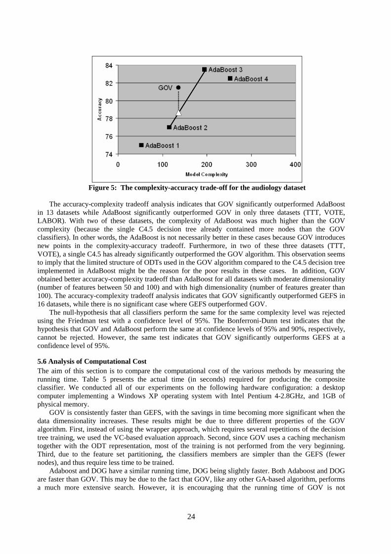
24
Figure 5: The complexity-accuracy trade-off for the audiology dataset
The accuracy-complexity tradeoff analysis indicates that GOV significantly outperformed AdaBoost
in 13 datasets while AdaBoost significantly outperformed GOV in only three datasets (TTT, VOTE, LABOR). With two of these datasets, the complexity of AdaBoost was much higher than the GOV complexity (because the single C4.5 decision tree already contained more nodes than the GOV classifiers). In other words, the AdaBoost is not necessarily better in these cases because GOV introduces new points in the complexity-accuracy tradeoff. Furthermore, in two of these three datasets (TTT, VOTE), a single C4.5 has already significantly outperformed the GOV algorithm. This observation seems to imply that the limited structure of ODTs used in the GOV algorithm compared to the C4.5 decision tree implemented in AdaBoost might be the reason for the poor results in these cases. In addition, GOV obtained better accuracy-complexity tradeoff than AdaBoost for all datasets with moderate dimensionality (number of features between 50 and 100) and with high dimensionality (number of features greater than 100). The accuracy-complexity tradeoff analysis indicates that GOV significantly outperformed GEFS in 16 datasets, while there is no significant case where GEFS outperformed GOV.
The null-hypothesis that all classifiers perform the same for the same complexity level was rejected using the Friedman test with a confidence level of 95%. The Bonferroni-Dunn test indicates that the hypothesis that GOV and AdaBoost perform the same at confidence levels of 95% and 90%, respectively, cannot be rejected. However, the same test indicates that GOV significantly outperforms GEFS at a confidence level of 95%.
5.6 Analysis of Computational Cost The aim of this section is to compare the computational cost of the various methods by measuring the running time. Table 5 presents the actual time (in seconds) required for producing the composite classifier. We conducted all of our experiments on the following hardware configuration: a desktop computer implementing a Windows XP operating system with Intel Pentium 4-2.8GHz, and 1GB of physical memory.
GOV is consistently faster than GEFS, with the savings in time becoming more significant when the data dimensionality increases. These results might be due to three different properties of the GOV algorithm. First, instead of using the wrapper approach, which requires several repetitions of the decision tree training, we used the VC-based evaluation approach. Second, since GOV uses a caching mechanism together with the ODT representation, most of the training is not performed from the very beginning. Third, due to the feature set partitioning, the classifiers members are simpler than the GEFS (fewer nodes), and thus require less time to be trained.
Adaboost and DOG have a similar running time, DOG being slightly faster. Both Adaboost and DOG are faster than GOV. This may be due to the fact that GOV, like any other GA-based algorithm, performs a much more extensive search. However, it is encouraging that the running time of GOV is not
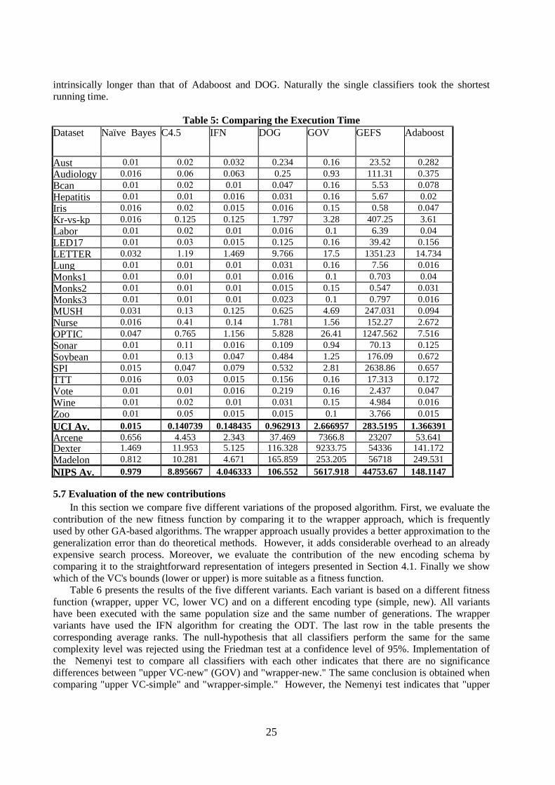
25
intrinsically longer than that of Adaboost and DOG. Naturally the single classifiers took the shortest running time.
Table 5: Comparing the Execution Time
Dataset Naïve Bayes C4.5 IFN DOG GOV GEFS Adaboost
Aust 0.01 0.02 0.032 0.234 0.16 23.52 0.282 Audiology 0.016 0.06 0.063 0.25 0.93 111.31 0.375 Bcan 0.01 0.02 0.01 0.047 0.16 5.53 0.078 Hepatitis 0.01 0.01 0.016 0.031 0.16 5.67 0.02 Iris 0.016 0.02 0.015 0.016 0.15 0.58 0.047 Kr-vs-kp 0.016 0.125 0.125 1.797 3.28 407.25 3.61 Labor 0.01 0.02 0.01 0.016 0.1 6.39 0.04 LED17 0.01 0.03 0.015 0.125 0.16 39.42 0.156 LETTER 0.032 1.19 1.469 9.766 17.5 1351.23 14.734 Lung 0.01 0.01 0.01 0.031 0.16 7.56 0.016 Monks1 0.01 0.01 0.01 0.016 0.1 0.703 0.04 Monks2 0.01 0.01 0.01 0.015 0.15 0.547 0.031 Monks3 0.01 0.01 0.01 0.023 0.1 0.797 0.016 MUSH 0.031 0.13 0.125 0.625 4.69 247.031 0.094 Nurse 0.016 0.41 0.14 1.781 1.56 152.27 2.672 OPTIC 0.047 0.765 1.156 5.828 26.41 1247.562 7.516 Sonar 0.01 0.11 0.016 0.109 0.94 70.13 0.125 Soybean 0.01 0.13 0.047 0.484 1.25 176.09 0.672 SPI 0.015 0.047 0.079 0.532 2.81 2638.86 0.657 TTT 0.016 0.03 0.015 0.156 0.16 17.313 0.172 Vote 0.01 0.01 0.016 0.219 0.16 2.437 0.047 Wine 0.01 0.02 0.01 0.031 0.15 4.984 0.016 Zoo 0.01 0.05 0.015 0.015 0.1 3.766 0.015
UCI Av. 0.015 0.140739 0.148435 0.962913 2.666957 283.5195 1.366391 Arcene 0.656 4.453 2.343 37.469 7366.8 23207 53.641 Dexter 1.469 11.953 5.125 116.328 9233.75 54336 141.172 Madelon 0.812 10.281 4.671 165.859 253.205 56718 249.531
NIPS Av. 0.979 8.895667 4.046333 106.552 5617.918 44753.67 148.1147
5.7 Evaluation of the new contributions In this section we compare five different variations of the proposed algorithm. First, we evaluate the
contribution of the new fitness function by comparing it to the wrapper approach, which is frequently used by other GA-based algorithms. The wrapper approach usually provides a better approximation to the generalization error than do theoretical methods. However, it adds considerable overhead to an already expensive search process. Moreover, we evaluate the contribution of the new encoding schema by comparing it to the straightforward representation of integers presented in Section 4.1. Finally we show which of the VC's bounds (lower or upper) is more suitable as a fitness function.
Table 6 presents the results of the five different variants. Each variant is based on a different fitness function (wrapper, upper VC, lower VC) and on a different encoding type (simple, new). All variants have been executed with the same population size and the same number of generations. The wrapper variants have used the IFN algorithm for creating the ODT. The last row in the table presents the corresponding average ranks. The null-hypothesis that all classifiers perform the same for the same complexity level was rejected using the Friedman test at a confidence level of 95%. Implementation of the Nemenyi test to compare all classifiers with each other indicates that there are no significance differences between "upper VC-new" (GOV) and "wrapper-new." The same conclusion is obtained when comparing "upper VC-simple" and "wrapper-simple." However, the Nemenyi test indicates that "upper

26
VC-new" significantly outperforms "lower VC-new" at confidence levels of 95%. Moreover "upper-VC-new" significantly outperforms "upper-VC-simple". Thus, we can conclude that:
1. The new encoding is better than the simple encoding. 2. The upper-VC based fitness function and the wrapper-based fitness function provide
equivalent accuracies. Since the upper-VC is much faster, it is preferable. 3. The VC lower bound is too "rough" to be used by the GA's fitness function.
It is well-known that VC dimension theory does not accurately evaluate generalization capabilities
(see, for instance, Ref [55]). However, the last result indicates that in our case using the upper VC dimension bound is sufficient. This is due to the fact that we are not interested in the accuracy itself, but use the bound only to compare solutions. Thus, the imprecision is less crucial, especially if in most of the cases the pair-wise dominance is retained, namely: if the generalized error of solution A is lower than that of solution B, then the VC bound of A is also lower than that of solution B. Moreover, because we take specific account of the restricted structure of decision tree (ODT), the obtained VC bound is tighter than those provided for a general decision tree. This makes this bound more applicable in practice than previous existing VC bounds.
Table 6: A comparison of five variants of the proposed algorithm. Each variant is defined based on a different fitness function (wrapper, upper VC, lower VC) and on a different encoding type (simple, new).
Fitness Function
Wrapper VC Upper Bound
Wrapper VC Lower Bound
VC Upper Bound
Encoding Simple Simple New New New
Aust 82.36±3.79 83.2±4.63 86.52±2.60 83.83±4.20 85.35±4.6 Audiology 78.95±2 78.1±3.2 81.68±3.89 77.25±4.09 81.5±4.29 Bcan 96.24±1.16 96.6±1.37 96.82±1.18 96.67±1.00 97.13±1.6 Hepatitis 79.1±2.1 79.9±2.12 83.67±5.41 76.15±5.09 81.29±5.46 Iris 92.86±3.66 94.09±3.04 94.87±3.34 94.47±3.38 96±3.33 Kr-vs-kp 98.37±0.68 98.45±0.49 99.35±0.31 99.27±0.63 99.44±0.35 Labor 94.13±3.67 94.2±3.61 95.64±3.66 94.54±3.66 95.17±3.5 LED17 70.68±3.49 69.35±4 73.67±3.20 70.97±3.69 72.36±3.7 LETTER 73.87±1.41 73.96±0.73 77.34±1.11 74.72±1.01 75.02±1.7 Lung 47.65 ±6.4 49.04±9.17 50.03±10.02 45.74±10.32 53.55±10.05 Monks1 97.5±1.9 98.33±1.12 98.67±0.76 98.41±1.55 98.51± 1.3 Monks2 58.4±7.23 57.37±7.31 63.48±7.42 58.91±7.62 61.56±7.6 Monks3 92±5.47 92.77±5.65 94.44±5.59 92.96±5.19 93.44±5.34 MUSH 99.17±1.2 99.17±1.2 100.00±0 100.00±0 100±0 Nurse 93.01±1.12 92.59±1.01 96.85±1.15 93.35±0.95 96.82±1.16 OPTIC 92.89±0.84 92.71±1.2 91.91±0.88 91.11±0.79 91.84±1.1 Sonar 74.84±2.61 74.8±2.57 75.60±2.68 75.20±2.71 76.42±3.23 Soybean 94.48±0.14 94.32±-0.15 95.04±0.53 94.57±0.27 94.95±0.4 SPI 95.3±0.12 95.7±0.96 96.31±0.16 96.00±0.53 96.3±0.7 TTT 78.04±2.39 77.82±2.17 80.04±2.30 78.76±2.28 80.24±2.7 Vote 90.77±2.94 89.63±2.69 94.16±2.56 90.99±2.92 93.79±2.8 Wine 93.05±4.28 93.02±4.13 94.27±3.90 93.98±4.25 95.92±4.41 Zoo 96.22±2.42 96.22±2.45 98.69±2.72 97.02±2.79 97.21±3.42 Arcene 67.69±6.36 71.21±6.33 73.43±6.60 71.87±6.73 77±7.2 Dexter 89.73±2.02 89.31±1.76 91.09±1.51 90.23±2.20 90.28±1.9
data
set
Madelon 68.89±5.12 68±4.34 71.87±2.38 67.59±3.14 71.2 ±2.9 Average Rank
4.2 4.22 1.42 3.37 1.77
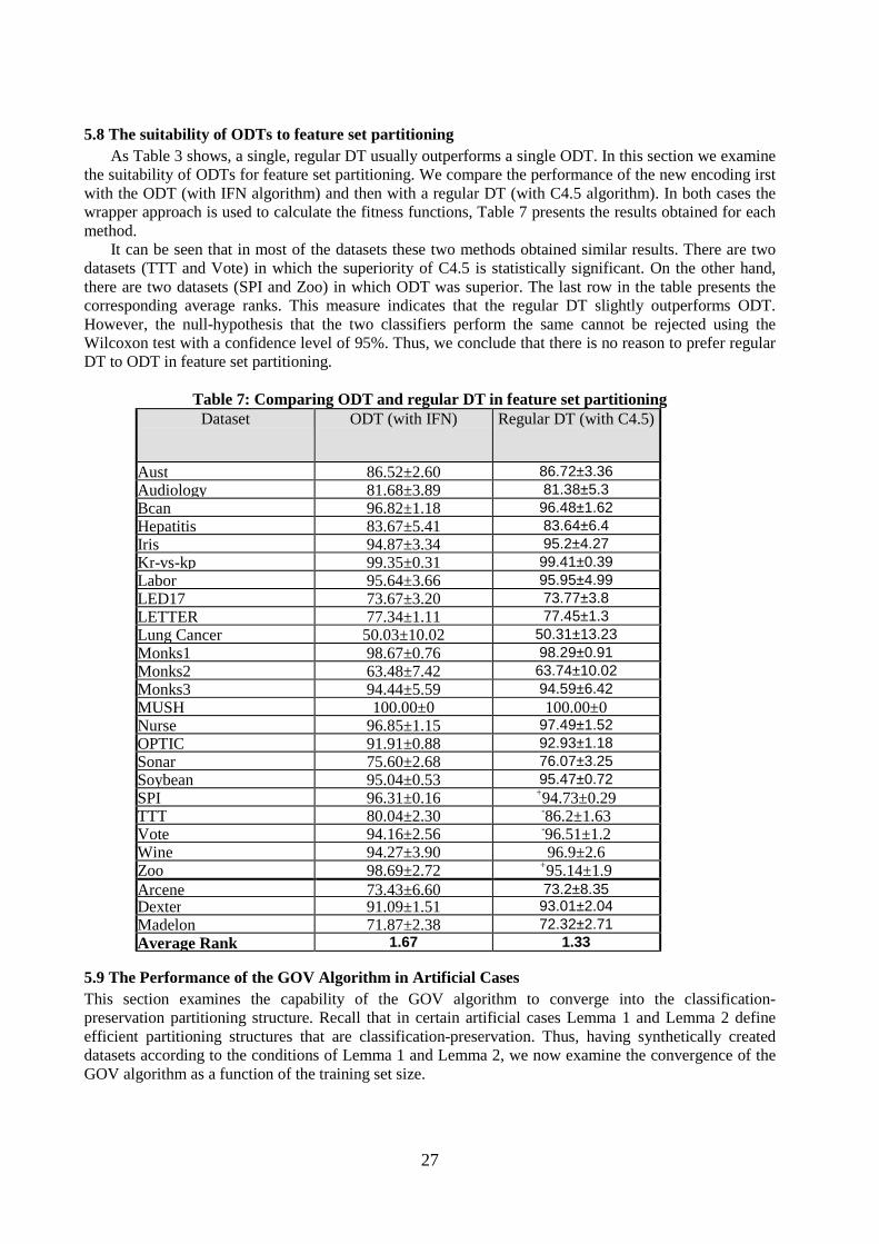
27
5.8 The suitability of ODTs to feature set partitioning As Table 3 shows, a single, regular DT usually outperforms a single ODT. In this section we examine
the suitability of ODTs for feature set partitioning. We compare the performance of the new encoding irst with the ODT (with IFN algorithm) and then with a regular DT (with C4.5 algorithm). In both cases the wrapper approach is used to calculate the fitness functions, Table 7 presents the results obtained for each method.
It can be seen that in most of the datasets these two methods obtained similar results. There are two datasets (TTT and Vote) in which the superiority of C4.5 is statistically significant. On the other hand, there are two datasets (SPI and Zoo) in which ODT was superior. The last row in the table presents the corresponding average ranks. This measure indicates that the regular DT slightly outperforms ODT. However, the null-hypothesis that the two classifiers perform the same cannot be rejected using the Wilcoxon test with a confidence level of 95%. Thus, we conclude that there is no reason to prefer regular DT to ODT in feature set partitioning.
Table 7: Comparing ODT and regular DT in feature set partitioning Dataset ODT (with IFN) Regular DT (with C4.5)
Aust 86.52±2.60 86.72±3.36 Audiology 81.68±3.89 81.38±5.3 Bcan 96.82±1.18 96.48±1.62 Hepatitis 83.67±5.41 83.64±6.4 Iris 94.87±3.34 95.2±4.27 Kr-vs-kp 99.35±0.31 99.41±0.39 Labor 95.64±3.66 95.95±4.99 LED17 73.67±3.20 73.77±3.8 LETTER 77.34±1.11 77.45±1.3 Lung Cancer 50.03±10.02 50.31±13.23 Monks1 98.67±0.76 98.29±0.91 Monks2 63.48±7.42 63.74±10.02 Monks3 94.44±5.59 94.59±6.42 MUSH 100.00±0 100.00±0 Nurse 96.85±1.15 97.49±1.52 OPTIC 91.91±0.88 92.93±1.18 Sonar 75.60±2.68 76.07±3.25 Soybean 95.04±0.53 95.47±0.72 SPI 96.31±0.16 +94.73±0.29 TTT 80.04±2.30 -86.2±1.63 Vote 94.16±2.56 -96.51±1.2 Wine 94.27±3.90 96.9±2.6 Zoo 98.69±2.72 +95.14±1.9 Arcene 73.43±6.60 73.2±8.35 Dexter 91.09±1.51 93.01±2.04 Madelon 71.87±2.38 72.32±2.71 Average Rank 1.67 1.33
5.9 The Performance of the GOV Algorithm in Artificial Cases This section examines the capability of the GOV algorithm to converge into the classification-preservation partitioning structure. Recall that in certain artificial cases Lemma 1 and Lemma 2 define efficient partitioning structures that are classification-preservation. Thus, having synthetically created datasets according to the conditions of Lemma 1 and Lemma 2, we now examine the convergence of the GOV algorithm as a function of the training set size.

28
The first group of synthetic datasets is based on read-once DNF functions (each variable appears at most once). This experiment examined 16 datasets. Each dataset is denoted by DNF(m,l), where m indicates the number of disjunctions and l the number of features in each disjunction. The input feature values were drawn from a uniform distribution. Note that the read-once DNF problem was investigated in the past and there are several polynomial time induction algorithms that are PAC-learnable under uniform distribution (see, for example, Ref [56]). It should be noted that, although these algorithms are very efficient in learning specific Boolean functions structures, they are limited in their capability to learn general domain problems as required in practice.
The second synthetic dataset group examined the ability of the proposed algorithms to converge to the optimal partitioning structure as presented in Lemma 1. All datasets in this group contained several binary input features and a binary class. The synthetic data were generated in such a manner that all features were relevant for modeling the class and the feature set could be divided into m conditionally independent groups of l features each. In order to obtain this synthetic dataset, the following procedure was performed for each class:
1. All input features were randomly allocated into m equally-sized groups of l features. 2. For each value combination (i) of each group (j) and for each value of the target feature, a value
10 ,, ≤≤ kjip is randomly selected such that 2
, ,1
1 ; ,l
i j ki
p j k=
= ∀∑ , where kjip ,, denotes the
probability of the features in group j to get the value combination i when the target feature obtains the value k. Note that, because in each group there are exactly l binary features, then there are 2l value combinations.
In order to fabricate one instance, the value of the target feature was sampled first (assuming uniform distribution). The values of all input features were then sampled according to the appropriate distribution.
Table 8 presents the results obtained by executing the GOV on each problem on different training set sizes. It can be seen that the partitioning structural distance (PSD) of GOV from the classification-preservation partitioning decreases with the size of the training set. Moreover, in simple cases having only three disjunctions, the distance algorithm converges to 0 with a training set of 400 instances. A similar observation can be identified in the INDEP datasets. The GOV algorithm converges to the classification-preservation partitioning as the training set size increases. When the problem is simpler (i.e., there are fewer features), then the distance is shorter for the same training set. This is not surprising because in larger problems the search space increases in an exponential manner. Evidently the GOV algorithm is capable of identifying the desired structure.
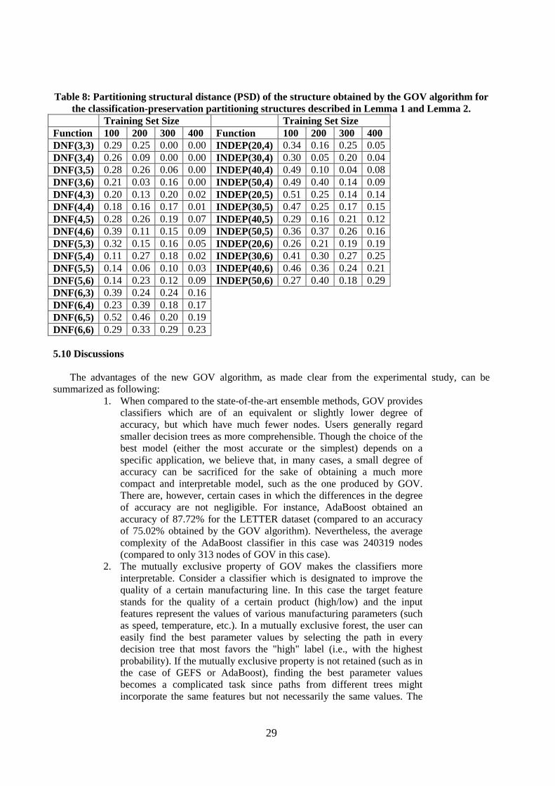
29
Table 8: Partitioning structural distance (PSD) of the structure obtained by the GOV algorithm for
the classification-preservation partitioning structures described in Lemma 1 and Lemma 2. Training Set Size Training Set Size Function 100 200 300 400 Function 100 200 300 400 DNF(3,3) 0.29 0.25 0.00 0.00 INDEP(20,4) 0.34 0.16 0.25 0.05 DNF(3,4) 0.26 0.09 0.00 0.00 INDEP(30,4) 0.30 0.05 0.20 0.04 DNF(3,5) 0.28 0.26 0.06 0.00 INDEP(40,4) 0.49 0.10 0.04 0.08 DNF(3,6) 0.21 0.03 0.16 0.00 INDEP(50,4) 0.49 0.40 0.14 0.09 DNF(4,3) 0.20 0.13 0.20 0.02 INDEP(20,5) 0.51 0.25 0.14 0.14 DNF(4,4) 0.18 0.16 0.17 0.01 INDEP(30,5) 0.47 0.25 0.17 0.15 DNF(4,5) 0.28 0.26 0.19 0.07 INDEP(40,5) 0.29 0.16 0.21 0.12 DNF(4,6) 0.39 0.11 0.15 0.09 INDEP(50,5) 0.36 0.37 0.26 0.16 DNF(5,3) 0.32 0.15 0.16 0.05 INDEP(20,6) 0.26 0.21 0.19 0.19 DNF(5,4) 0.11 0.27 0.18 0.02 INDEP(30,6) 0.41 0.30 0.27 0.25 DNF(5,5) 0.14 0.06 0.10 0.03 INDEP(40,6) 0.46 0.36 0.24 0.21 DNF(5,6) 0.14 0.23 0.12 0.09 INDEP(50,6) 0.27 0.40 0.18 0.29 DNF(6,3) 0.39 0.24 0.24 0.16 DNF(6,4) 0.23 0.39 0.18 0.17 DNF(6,5) 0.52 0.46 0.20 0.19 DNF(6,6) 0.29 0.33 0.29 0.23 5.10 Discussions
The advantages of the new GOV algorithm, as made clear from the experimental study, can be
summarized as following: 1. When compared to the state-of-the-art ensemble methods, GOV provides
classifiers which are of an equivalent or slightly lower degree of accuracy, but which have much fewer nodes. Users generally regard smaller decision trees as more comprehensible. Though the choice of the best model (either the most accurate or the simplest) depends on a specific application, we believe that, in many cases, a small degree of accuracy can be sacrificed for the sake of obtaining a much more compact and interpretable model, such as the one produced by GOV. There are, however, certain cases in which the differences in the degree of accuracy are not negligible. For instance, AdaBoost obtained an accuracy of 87.72% for the LETTER dataset (compared to an accuracy of 75.02% obtained by the GOV algorithm). Nevertheless, the average complexity of the AdaBoost classifier in this case was 240319 nodes (compared to only 313 nodes of GOV in this case).
2. The mutually exclusive property of GOV makes the classifiers more interpretable. Consider a classifier which is designated to improve the quality of a certain manufacturing line. In this case the target feature stands for the quality of a certain product (high/low) and the input features represent the values of various manufacturing parameters (such as speed, temperature, etc.). In a mutually exclusive forest, the user can easily find the best parameter values by selecting the path in every decision tree that most favors the "high" label (i.e., with the highest probability). If the mutually exclusive property is not retained (such as in the case of GEFS or AdaBoost), finding the best parameter values becomes a complicated task since paths from different trees might incorporate the same features but not necessarily the same values. The

30
user is compelled to resolve these conflicts, if she wants to best tune the manufacturing process.
3. In GOV, the decision trees are based on the original distribution of the training set. The class distribution at the tree's leafs is supported by the training set. In Adaboost (starting from the second decision tree) and in GEFS, the class distribution at the leaf level does not necessarily fit the original distribution. This makes it difficult to justify the results to a non- professional user.
4. The new algorithm is faster than existing GA-based ensembles methods for to the following two reasons: a. The fitness function uses a VC dimension bound, which is faster
than the wrapper estimation. b. A new caching mechanism reduces the need to build ODT from
scratch. 5. The new encoding schema is more efficient than straightforward
encoding, because it provides better results for the same population size and number of generations.
6. The use of ODT as the base classifier provides reasonable results. 7. In artificial cases, we have shown that the GOV algorithm usually almost
converges to the optimal partitioning. The GOV algorithm has also several drawbacks:
1. It is slower than non-GA feature set partitioning methods. 2. The fact that it is specifically designed for an ODT is considered to be its
Achilles' heel. Potentially, there might be domains in which using the ODT as the base classifier will dramatically reduce accuracy. A partial solution in such cases would be to use ODTs internally as an agile inducer only for the feature set partitioning phase. Subsequently, when a good partition is obtained, we can employ more sophisticated inducers on each subset. Similarly, as stated in Section 2, a single ODT has been used for the preprocess phase of feature selection.
6. Conclusions In this paper, we have presented a novel genetic algorithm for finding the best mutually exclusive feature set partitioning. The basic idea is to decompose the original set of features into several subsets, build a decision tree for each projection, and then combine them. This paper examines whether genetic algorithms can be useful for discovering the appropriate partitioning structure.
For this purpose we suggested a new encoding schema and fitness function that were specially designed for feature set partitioning with oblivious decision trees. Additionally a caching mechanism was implemented in order to reduce computational cost.
The algorithm was evaluated on a wide range of standard datasets containing continuous, categorical, and binary-valued attributes. The results show that this algorithm outperforms other state-of-the-art ensemble methods in the accuracy-complexity trade-off. This observation leads us to conclude that the proposed algorithm can be used for creating compact ensemble structures.
Additional issues to be further studied include: how the feature set partitioning concept can be implemented with other inducers such as neural networks and other techniques for combining the generated classifiers (such as voting). Acknowledgments The author gratefully thanks the action editor and the anonymous reviewers whose constructive comments helped in improving the quality and accuracy of this paper.

31
References
1. L. O. Jimenez,, D. A. Landgrebe, Supervised Classification in High- Dimensional Space: Geometrical, Statistical, and Asymptotical Properties of Multivariate Data. IEEE Transaction on Systems Man, and Cybernetics — Part C: Applications and Reviews, 28 (1998): pp 39-54.
2. K. Fukunaga, Introduction to Statistical Pattern Recognition. San Diego, CA: Academic, 1990.
3. J. Hwang, S. Lay, A. Lippman, Nonparametric multivariate density estimation: A comparative study, IEEE Transaction on Signal Processing, 42 (1994), pp 2795-2810.
4. R. Bellman, Adaptive Control Processes: A Guided Tour, Princeton University Press, 1961. 5. I. Guyon, S. Gunn, M. Nikravesh, and L. Zadeh, Feature Extraction, Foundations and
Applications, Series Studies in Fuzziness and Soft Computing, Physica-Verlag, Springer, 2006.
6. D. Opitz, and R. Maclin, Popular Ensemble Methods: An Empirical Study, Journal of Artificial Research, 11 (1999): 169-198.
7. S. Geman, E. Bienenstock, and R. Doursat, R., Neural networks and the bias/variance dilemma. Neural Computation, 4 (1995):1-58.
8. K. Tumer, and J. Ghosh, Linear and Order Statistics Combiners for Pattern Classification, in Combining Articial Neural Nets, A. Sharkey (Ed.), pp. 127-162, Springer-Verlag, 1999.
9. L. Breiman, Bagging predictors, Machine Learning, 24 (1996):123-140. 10. Y. Freund, and Schapire R., Experiments with a New Boosting Algorithm. Machine
Learning: Proceedings for the Thirteenth International Conference, Morgan Kaufmann, San Francisco, 1996, pp. 148-156.
11. K. Tumer, C. N. Oza, Input decimated ensembles. Pattern Analysis and Application 6 (2003) 65-77.
12. R. Bryll, Gutierrez-Osuna R., Quek F., Attribute bagging: improving accuracy of classifier ensembles by using random feature subsets, Pattern Recognition Volume 36 (2003): 1291-1302
13. T. K. Ho, The random subspace method for constructing decision forests, IEEE Transactions On Pattern Analysis And Machine Intelligence, 20(1998): 832-844.
14. S. Bay, Nearest neighbor classification from multiple feature subsets. Intelligent Data Analysis, 3(1999): 191-209.
15. A. Tsymbal, and S. Puuronen, Ensemble Feature Selection with the Simple Bayesian Classification in Medical Diagnostics, In: Proc. 15thIEEE Symp. on Computer-Based Medical Systems CBMS’2002, Maribor, Slovenia, IEEE CS Press, 2002, pp. 225-230.
16. Q. X. Wu , D. Bell and M. McGinnity, Multi-knowledge for decision making, Journal Knowledge and Information Systems, 7(2005): 246-266
17. Y Bao, N. Ishii, Combining multiple K-nearest neighbor classifiers for text classification by reducts. In: Proceedings of 5th international conference on discovery science, LNCS 2534, Springer, 2002, pp 340–347
18. Q. H. Hu, D. R. Yu, M. Y. Wang, Constructing Rough Decision Forests, D. Slezak et al. (Eds.): RSFDGrC 2005, LNAI 3642, Springer, 2005, pp. 147-156
19. P. Cunningham, and J. Carney, Diversity Versus Quality in Classification Ensembles Based on Feature Selection, In: R. L. de Mántaras and E. Plaza (Eds.), Proc. ECML 2000, Barcelona, Spain, LNCS 1810, Springer, 2000, pp. 109-116.
20. G. Zenobi, and P. Cunningham, Using diversity in preparing ensembles of classifiers based on different feature subsets to minimize generalization error, In: In L. De Readt & P. Flach (Eds.), Proc. ECML 2001, LNAI 2167, Springer, 2001, pp. 576-587.
21. A. Tsymbal, M. Pechenizkiy, P. Cunningham, Diversity in search strategies for ensemble feature selection. Information Fusion 6(2005): 83-98.
22. S. Gunter, H. Bunke, Feature Selection Algorithms for the generation of multiple classifier systems, Pattern Recognition Letters, 25(2004):1323-1336.
32
23. L. Rokach, Decomposition Methodology for Classification Tasks - A Meta Decomposer Framework, Pattern Analysis & Applications, 9(2006):257-271.
24. A. Kusiak, Decomposition in Data Mining: An Industrial Case Study, IEEE Transactions on Electronics Packaging Manufacturing, 23(2000): 345-353.
25. F. J.Provost, and V. Kolluri, A Survey of Methods for Scaling Up Inductive Learning Algorithms, Proc. 3rd International Conference on Knowledge Discovery and Data Mining, 1997.
26. A. Sharkey, On combining artificial neural nets, Connection Science, 8 (1996): 299-313. 27. P. K. Chan and S. J. Stolfo, On the Accuracy of Meta-learning for Scalable Data Mining, J.
Intelligent Information Systems, 8 (1997):5-28. 28. J. Gama, A Linear-Bayes Classifier. In C. Monard (Ed.), Advances on Artificial Intelligence --
Proc. SBIA 2000, LNAI 1952, Springer, 2000, pp 269-279. 29. K. Tumer, and J. Ghosh, Error Correlation and Error Reduction in Ensemble Classifiers,
Connection Science, Special issue on combining artificial neural networks: ensemble approaches, 8 (1996): 385-404.
30. K. J. Cherkauer, Human Expert-Level Performance on a Scientific Image Analysis Task by a System Using Combined Artificial Neural Networks. In In Chan, P. (Ed.), Working Notes, Integrating Multiple Learned Models for Improving and Scaling Machine Learning Algorithms Workshop, Thirteenth National Conference on Artificial Intelligence. Portland, OR: AAAI Press, 1996, pp. 15-21
31. K. Chen, L. Wang and H. Chi, Methods of Combining Multiple Classifiers with Different Features and Their Applications to Text-Independent Speaker Identification, International Journal of Pattern Recognition and Artificial Intelligence, 11(1997): 417-445.
32. Y. Liao, and J. Moody, Constructing Heterogeneous Committees via Input Feature Grouping, in S.A. Solla, T.K. Leen and K.-R. Muller (Eds.), Advances in Neural Information Processing Systems, Vol.12, MIT Press, 2000.
33. L. Rokach and O. Maimon, Feature Set Decomposition for Decision Trees, Journal of Intelligent Data Analysis, 9(2005):131-158.
34. A. Freitas A., Evolutionary Algorithms for Data Mining, in O. Maimon and L. Rokach (Eds.), The Data Mining and Knowledge Discovery Handbook, Springer, 2005, pp. 435-467.
35. D. Opitz, Feature Selection for Ensembles, In: Proc. 16th National Conf. on Artificial Intelligence, AAAI, 1999, pp. 379-384.
36. S. J. Louis and G. J. E. Rawlins. Predicting convergence time for genetic algorithms. In L. D. Whitley, (Ed.), Foundations of Genetic Algorithms 2, Morgan Kaufmann, 1993, pp. 141-161.
37. W. M. Rand, Objective criteria for the evaluation of clustering methods. Journal of the American Statistical Association, 66 (1971): 846–850.
38. P.K. Sharpe and R.P Glover., Efficient GA based techniques for classification, Applied Intelligence, 11 (1999): 277-284,.
39. M. Kudo and J. Sklansky, Comparison of algorithms that select features for pattern classifiers, Pattern Recognition 33(2000): 25-41.
40. W. H. Hsu, Genetic wrappers for feature selection in decision tree induction and variable ordering in Bayesian network structure learning. Information Sciences, 163(2004):103-122.
41. D. Opitz, and J. Shavlik,. Actively searching for an effective neural-network ensemble. Connection Science 8(1996):337-353.
42. W. H. Hsu, M. Welge, J. Wu, T. Yang, Genetic algorithms for selection and partitioning of features in large-scale data mining problems, in: Proceedings of the Joint AAAI-GECCO Workshop on Data Mining with Evolutionary Algorithms, Orlando, FL, July 1999.
43. Wolpert, D. H., The relationship between PAC, the statistical physics framework, the Bayesian framework, and the VC framework. In D. H. Wolpert, editor, The Mathematics of Generalization, The SFI Studies in the Sciences of Complexity, pages 117-214. Addison-Wesley, 1995.
33
44. Y. Mansour, and D. McAllester, Generalization Bounds for Decision Trees, in Proceedings of the 13th Annual Conference on Computer Learning Theory, San Francisco, Morgan Kaufmann, 2000, pp. 69-80.
45. H. Fröhlich, O. Chapelle, B. Schölkopf, Feature Selection for Support Vector Machines using Genetic Algorithms, International Journal on Artificial Intelligence Tools, 13(2004):791-800,
46. J. R. Quinlan, C4.5: Programs for Machine Learning, Morgan Kaufmann, 1993. 47. R. Duda, P. Hart, 1Pattern Classification and Scene Analysis, New-York, Wiley, 1973. 48. H. Almuallim, and T.G. Dietterichm, Learning Boolean concepts in the presence of many
irrelevant features. Artificial Intelligence, 69(1994): 279-306. 49. J. C. Schlimmer, Efficiently inducing determinations: A complete and systematic search
algorithm that uses optimal pruning. In Proceedings of the 1993 International Conference on Machine Learning, San Mateo, CA, Morgan Kaufmann, 1993, pp. 284-290.
50. P. Langley, and S. Sage, Induction of selective Bayesian classifiers. in Proceedings of the Tenth Conference on Uncertainty in Artificial Intelligence, Seattle, WA: Morgan Kaufmann, 1994, pp. 399-406.
51. Last M., Maimon M., A Compact and Accurate Model for Classification, IEEE Transactions On Knowledge And Data Engineering, 16(2004):203-215
52. N. V. Chawla, L. O. Hall, K. W. Bowyer, W. P. Kegelmeyer, Learning Ensembles from Bites: A Scalable and Accurate Approach, Journal of Machine Learning Research 5 (2004): pp. 421-451.
53. C. J Merz, and P.M. Murphy, UCI Repository of machine learning databases. Irvine, CA: University of California, Department of Information and Computer Science, 1998.
54. J. Demsar, Statistical Comparisons of Classifiers over Multiple Data Sets, Journal of Machine Learning Research, 7 (2006):1-30.
55. S.B. Holden and M Niranjan, On the practical applicability of VC dimension bounds Neural Computation, 7 (1995): 1265-1288.
56. M. Kearns, M. Li, and L. Valiant, Learning Boolean formulas, J. ACM 41(1994): 1298-1328. 57. C. S. Wallace, MML Inference of Predictive Trees, Graphs and Nets. In A. Gammerman (ed),
Computational Learning and Probabilistic Reasoning, Wiley 1996, pp 43-66. 58. M. Schmitt, On the complexity of computing and learning with multiplicative neural
networks, Neural Computation 14(2002): 241-301.

34
Appendix: Proofs
A.1. Proof of Lemma 1
( ) ( )1
kk
j j A jNR G
P y c P y c P y c ωπ π=
∪
= = = = =
x x xq q q∪
.
According to Bayes' theorem:
( )1
( )k
k
j jNR G
P y c P y c
P
ωπ=
∪
= = =
xq
xq
∪.
Using the independence assumption:
( ) ( )( )
1
( )kNR j G j j
k
P y c P y c P y c
P
ω
π π=
= ⋅ = == =
∏x xq q
xq
.
Using Bayes' theorem again, the last term becomes:
( ) ( )( ) ( ) ( )
1( )G kk
j NR NR
j Gkj
P y c PP y c P
P y c P
ω
ω
π ππ π
=
==
= ⋅∏
x xq qx xq q
xq
.
Due to the fact that the NR set and the target feature are independent:
( ) ( ) ( )( )
1
1( )
k kNR j G Gk
j
P P y c P
P y c P
ω
ω
π π π=
−
⋅ = ⋅=
= ⋅
∏x x xq q q
xq
.
As the value of the expression
1
( ) ( )
( )
kNR Gk
P P
P
ω
π π=
⋅∏x xq q
xq
is constant given specific values of the input features
( )arg max ( )
j
jc dom y
P y c∈
= =qx 11
( )
( )arg max
( )
k
j
j Gk
c dom y j
P y c
P y c
ω
ω
π=
−∈
=
=
∏ xq
i.e., Z is classification-preservation.
A.2. Proof of Lemma 2
It is obvious that all input features which do not belong to any of the sets 1,...,G Gω can be ignored. The
proof begins by showing that if y fulfills 1 1( ) ... ( )y f G f Gω ω= ∨ ∨ and that the values of the functions
are independent, then the partitioning 1{ ,..., }Z G Gω= is classification-preservation.

35
For the sake of simplicity we will denote ( )kk Gf π x as kf
Case 1: At least one of the functions of the instance to be classified gets the value 1. Because such a
function also fulfills ( 0 1) 0kP y f= = = :
( )1
1( ) ( )
, 1 arg max 1 arg max ( )( )j j
j kk
k jc dom y c dom yj
P y c fk f P y c
P y c
ω
ω=
−∈ ∈
=∃ = = = =
=
∏x .
Case 2: The values of the functions of the instance to be classified are all zeros.
In this case ( )1( 0) 0 ... 0P y P f fω= = = ∩ ∩ = . Due to the fact that the input features are independent:
( )1
( 0) 0ii
P y P fω
=
= = =∏
Furthermore: ( ) ( )0 0 0i kk i
P y f P f≠
= = = =∏
According to the complete probability theorem:
( )1
( 1) 1 0ii
P y P fω
=
= = − =∏
and
( ) ( )1 0 1 0i kk i
P y f P f≠
= = = − =∏ .
What is left to prove is:
( )
( )
( )
( )
111 1
{0,1}
1 1
1 00arg max , 0
0 1 0
kki k ii k i
y
i ii i
P fP f
P f P f
ωω
ω ωω ω
= ≠= ≠− −
∈
= =
− = = = = − =
∏ ∏∏∏
∏ ∏.
As the first argument of the argmax function equals one, it is required to show that:
( )
( )
11
1
1 0
1
1 0
ki k i
ii
P f
P f
ω
ωω
= ≠−
=
− = <
− =
∏ ∏
∏.
The last inequality can be validated by multiplying the numerator and denominator by
( )1
1 0ii
P fω
=
− =
∏ with the assumption that ( )1
1 1 0 0ii
P fω
=
> − = >
∏ .
(Note: If the term is equal to 0, then ( 1) 0P y = = and if the term is equal to 1 then ( 1) 1P y = = . In both cases the partitioning Z is classification-preservation.)
( ) ( )
( ) ( )
1 11
1 1
1 0 1 0
1 0 1 0
i ki i k i
i ii i
P f P f
P f P f
ω ω
ωω ω
= = ≠−
= =
− = ⋅ − = = − = ⋅ − =
∏ ∏ ∏
∏ ∏

36
( )( )
( )1 1
1
1 0
1 0
1 0
kk i
ii i
jj
P f
P f
P f
ω ω
ω≠
= =
=
− = − = ⋅ − =
∏∏ ∏
∏.
Because ( ) ( )1
0 0k jk i j
P f P fω
≠ =
= ≥ =∏ ∏ :
( )
( )1
1
1 0
1
1 0
kk i
i
jj
P f
P f
ω
ω≠
=
=
− = ≤
− =
∏∏
∏
or:
( )( )
( )1 1
1
1 0
1 0 1
1 0
kk i
ii i
jj
P f
P f
P f
ω ω
ω≠
= =
=
− = − = ⋅ < − =
∏∏ ∏
∏
To complete the proof, it is required to show that it is true also for the case of
1 1 2 2( ) ( ) ... ( )y f G f G f Gω ω= ∧ ∧ ∧ .
For this purpose it is sufficient to show that it is true for the opposite target feature y . According to Morgan's law:
1 1 2 2( ) ( ) ... ( )y f G f G f Gω ω= ∨ ∨ ∨
1 1 2 2
* * *1 1 2 2
( ) ( ) ... ( )
( ) ( ) ... ( )
y f G f G f G
f G f G f G
ω ω
ω ω
= ∨ ∨ ∨ =
∨ ∨ ∨.
Because Z is classification-preservation for y it is classification-preservation for y as well.
A.3. Proof of Lemma 3 In order to prove this lemma it is useful to define the following functions:
1( , ) th bit of x = ( 2 / 2 ) / 2i i ibit i x The x xι − = − ⋅ )1()1(),( yxyxyxXNOR −⋅−+⋅=
1 11 1
( ) ( )
( ) ( )arg max arg max
( ) ( )j j
j k j kk k
c dom y c dom yj j
P y c G P y c f
P y c P y c
ω ω
ω ω= =
− −∈ ∈
= ==
= =
∏ ∏
11
( )
{ ( , ( , )) ( ( , ) )}arg max
( )j
k j j jk
c dom y j
XNOR f bit k c P f bit j c j k
P y c
ω
ω=
−∈
⋅ = ∀ ≠=
=
∏.
As the input features are independent:

37
1
1( )
{ ( , ( , )) ( ( , ))}
arg max( )j
k j j jk j k
c dom y j
XNOR f bit k c P f bit j c
P y c
ω
ω= ≠
−∈
⋅ ==
=
∏ ∏
1
1 11
( )
( ( , )) ( , ( , ))arg max
( )j
j j k jk k
c dom y j
P f bit j c XNOR f bit k c
P y c
ω ωω
ω
−
= =−
∈
= ⋅=
=
∏ ∏
1
11
( )
( ) ( , ( , ))arg max
( )j
j k jk
c dom y j
P y c XNOR f bit k c
P y c
ωω
ω
−
=−
∈
= ⋅=
=
∏
( ) ( )1
arg max ( , ( , )) arg max ( )j j
k j jc dom y c dom yk
XNOR f bit k c P y cω
∈ ∈=
= = =∏ x .
A.4. Proof of Lemma 4
Obviously if { }Z A≠ then Z contains at least one subset. If there are an odd number of input features with the value "1" then the target feature should get the value "1" as well. For that reason the posteriori probability for the target feature to get "1" given only subset of the input feature set is ½.
1( 1 )
2P y S A= ⊂ = .
That is to say:
1 11 1
( 1 ) ( 0 )1
( 1) ( 0)
k kG Gk k
P y P y
P y P y
ω ω
ω ω
π π= =
− −
= == =
= =
∏ ∏x x.
A.5. Proof of Lemma 5 The proof of the first property of Lemma 5 results explicitly from definition. So does the proof of the first
direction of property 2 of Lemma 5, namely, if 21 ZZ = then 0),( 21 =ZZδ .
The opposite direction, namely if 0),( 21 =ZZδ then 21 ZZ = , is proved by contradiction. We assume
that there are cases where 0),( 21 =ZZδ but 21 ZZ ≠ . If 21 ZZ ≠ then without loss of generality 11 ZGi ∈∃ such that there is no 22 ZG j ∈ which fulfill
21ji GG = . Consequently ji aa ,∃ such that
1),,,( 21 =ZZaa jiη , which contradict the assumption and therefore our original assumption that
0),( 21 =ZZδ but 21 ZZ ≠ must be false. In order to prove property 3 of Lemma 5, note that:
∑ ∑−
= += −⋅+
⋅=+1
1 1
32313231
)1(
),,,(),,,(2),(),(
n
i
n
ij
jiji
nn
ZZaaZZaaZZZZ
ηηδδ .
Because the following arguments hold:
1. If 0),,,(),,,( 3231 =+ ZZaaZZaa jiji ηη then 0),,,( 21 =ZZaa jiη
2. If 2),,,(),,,( 3231 =+ ZZaaZZaa jiji ηη then 0),,,( 21 =ZZaa jiη

38
3. If 1),,,(),,,( 3231 =+ ZZaaZZaa jiji ηη then 1),,,( 21 =ZZaa jiη .
Then also the triangular inequality is true.
A.6. Proof of Lemma 6 A projection of matrix is obtained by removing certain features (i.e., removing their corresponding
rows and columns). Without the loss of generality, we assume that the removed features are the last t features. Let us assume by contradiction that the projected matrix is not well-defined but that the original matrix is well-defined. Because the projected matrix is not well-defined then , ,i j k n t∃ ≤ − . This violates one of the constraints specified in definition 3. However, because the original matrix is well-defined then for , ,i j k n∀ ≤ or more specifically for , ,i j k n t∀ ≤ − the above constraints hold. We have reached a contradiction and therefore our original assumption according to which the projected matrix is not well-defined, is not true.
A.7. Proof of Lemma 7 If the GWC operator is used then the new offspring are obtained by diagonally concatenating the projections of the anchor subset from one parent and the remaining features from the second parent. Based on Lemma 6, because the parents were well-defined so are their projections. It remains to show that the elements that are not obtained from the projection do not violate definition 3. We denote by R the original feature index of the anchor subset in the set A. Because the rows and the columns of the anchor subset R are copied as is, then Bi,j= Bj,i=0 for ;i R j R∀ ∈ ∉ . Therefore constraint 1 in definition 3 is always true and constraints 2 and 3 are not relevant in this case.
A.8. Proof of Lemma 8 We denote by Z1 and Z2 the parent solutions and by Z3 and Z4 the offspring. Because each element of the offspring is obtained from one of the parent then,
3 1 3 2 1 2( , ) ( , ) ( , )Z Z Z Z Z Zδ δ δ+ = 4 1 4 2 1 2( , ) ( , ) ( , )Z Z Z Z Z Zδ δ δ+ = .
The last equation is true because in Equation (7), the term 1 2( , , , ) 0i ja a Z Zη = if Bi,j in both matrices
are equal. Using the triangular inequality we obtain that:
3 4 3 1 4 1( , ) ( , ) ( , )Z Z Z Z Z Zδ δ δ≤ + 3 4 3 2 4 2( , ) ( , ) ( , )Z Z Z Z Z Zδ δ δ≤ + .
Thus:
3 4 3 1 4 1 3 2 4 22 ( , ) ( , ) ( , ) ( , ) ( , )Z Z Z Z Z Z Z Z Z Zδ δ δ δ δ≤ + + + or:
3 3 1 2( , ) ( , )Z Z Z Zδ δ≤ .

39
A.9. Proof of Theorem 1 To prove Theorem 1, it is useful to consider Lemma 9 and Lemma 10 first.
Lemma 9: The VC dimension of an oblivious decision tree on n binary input features with l layers and t terminal nodes is not greater than:
2
! (2 4)!log ( )
( )! ( 2)! ( 2)!
n tt
n l t t
−+ ⋅− − ⋅ −
.
Proof of Lemma 9: Any oblivious decision tree can be converted to a suitable classification tree with leaves labeled {0,1} according to the highest weight of each of the terminal nodes in the original tree. Because the probabilistic oblivious tree and its corresponding classification tree shatter the same subsets, their VC dimensions are identical.
The hypothesis space size of a classification oblivious tree with l layers, t terminal nodes and n input features to choose from is not greater than:
)!2()!2(
)!42(2
)!(
!
−⋅−−⋅⋅
− tt
t
ln
n t
. The first multiplier indicates the number of combinations for selecting with order l features from n.
The second multiplier corresponds to the different classification options of the terminal nodes. The third multiplier represents the number of different binary tree structures that contain t leaves. The last multiplier is calculated using the Wallace [57] tree structure. Note that in the case of the binary tree there is exactly one more leaf than inner nodes. Furthermore, the tree string always begins with an inner node
(when 1l ≥ ) and end with at least two leaf nodes. Based on the familiar relation 2( ) log ( )VC H H≤ for
finite H, the lemma has been proved.
Lemma 10: Consider ω mutually exclusive oblivious decision trees that are combined with the
naïve Bayes and that have a fixed structure containing 1( ,..., )T t tω=�
terminal nodes. The number
of dichotomies it induces on a set of cardinality m is at most:
∑
+
=
+
=∑
ω
ω
1
1
1
12
iit
iit
em
. Proof of Lemma 10: The proof of this lemma, uses a similar lemma introduced by Schmitt [58]: the number of dichotomies that a higher order threshold neuron with k monomials induces on a set of cardinality m is at most
0
12 2
kk
i
m em
i k=
− <
∑ for 1m k> ≥ .
A definition of a higher-order threshold neuron has the form:
1 1 2 2 ... k k rw M w M w M t+ + + −
where 1 2, ,..., kM M M are monomials.

40
ω oblivious decision trees which are combined with naïve Bayes can be converted to a higher order
threshold neuron, where the set of terminal nodes constitutes the neuron's monomials and the log-odds in favor of 1y = in each terminal node is the corresponding neuron's weight. Furthermore, in order to use the sign activation function, the threshold has been set to the sum of all other monomials.
Now it is possible to prove Theorem 1. The proof of the upper bound is discussed first. If 1ω = ,
then Lemma 9 can be used directly. For the case 1ω > , the bound of the number of dichotomies induced by ω mutually exclusive oblivious decision trees on an arbitrary set of cardinality m is first introduced. Because the biggest shattered set follows this bound as well, the statement of the theorem is derived.
There are at most:
∏∑ =
=
−⋅−−⋅
−⋅
ω
ω
ω 1
1
)!2()!2(
)!42(
)!(!
!
i ii
i
ii
tt
t
ln
n
different structures for ω mutually exclusive oblivious trees on n binary input features with
1( ,..., )L l lω=�
layers and 1( ,..., )T t tω=�
terminal nodes. Notice that the division by !ω is required as
there is no relevance to the order of the trees.
According to Lemma 10, a fixed structure and variable weights can induce at most:
1
1
1
21
ii
t
ii
em
t
ω
ω
=
+
=
∑ +
∑
dichotomies on a given set of cardinality m. Enumerating over all structures, it is concluded that there are at most:
1
1
1 1
(2 4)!!2
( 2)! ( 2)!! ( )! 1
ii
t
i
i i ii i
i i
tn em
t tn l t
ω
ω
ω ω
ω
=
=
= =
∑ − ⋅ ⋅
− ⋅ − ⋅ − +
∏∑ ∑
dichotomies on a given set of cardinality m that are induced by the class considered. If the above class shatters the given set, then:
∑
+⋅
−⋅−−⋅
−⋅≤
=
+
=
=
=∑
∏∑
ω
ω
ω
ω
ω
1
1
1
1
1
12
)!2()!2(
)!42(
)!(!
!2
iit
ii
i ii
i
ii
m
t
em
tt
t
ln
n
.

41
However, the last inequality will not be true if 2 ( 1) log(2 ) 2 logm F e U≥ • + + where 1
ii
F tω
=
=∑ and
1
1
(2 4)!!
( 2)! ( 2)!! ( )!
i
i i ii
i
tnU
t tn l
ω
ω
ω =
=
−= ⋅− ⋅ −⋅ −
∏∑
.
The lower bound is true due to the fact that any set of ω trees with a fixed structure has the above
VC dimension. The result can be achieved by setting in each tree (besides one) a neutralized terminal node (i.e., a terminal node with posteriori probabilities that are equal to the a-priori probabilities). This concludes the proof.