genetic algorithm and its variants: theory and...

1

GENETIC ALGORITHM AND ITS VARIANTS: THEORY

AND APPLICATIONS

B.TECH FINAL YEAR

PROJECT REPORT

NAME: BINEET MISHRA NAME: RAKESH KUMAR PATNAIK

ROLL NO: 10509033 ROLL NO: 10507002

GUIDE: Dr. G.PANDA

Department of Electronics and Communication Engineering.

NIT ROURKELA

2

CERTIFICATE:

This is to certify that the project report entitled “Genetic Algorithm and its variants: Theory

and Applications” is a bonafide work done by BINEET MISHRA, Final year student of

Electronics and Communication Engineering, Roll No.:10509033 and RAKESH KUMAR

PATNAIK, Final year student of Electronics and Instrumentation Engineering, Roll

No.:10507002 at NATIONAL INSTITUTE OF TECHNOLOGY, ROURKELA during their

final year.

Dr. G.PANDA

Project Guide

National Institute of Technology,

Rourkela.

DATE:

3

ACKNOWLEDGEMENT:

We wish to express our sincere thanks and gratitude to Dr.G.PANDA, Professor, Department of

Electronics and Communication Engineering, NIT ROURKELA, for the stimulating discussions,

in analyzing problems associated with our project work and for guiding us throughout the

project. Project meetings were highly informative. We express our warm and sincere thanks for

the encouragement, untiring guidance and the confidence he had shown in us. We are immensely

indebted for his invaluable guidance throughout our project.

We also thank Mr.Pyari Mohan Pradhan, M.Tech, and Mr.Jaganath Nanda, PhD Scholar of NIT

ROURKELA for helping us out during the execution of our project.

Finally, we would also like to thank our parents and friends for constant encouragement and help

throughout the course of the project.

Bineet Mishra Rakesh Kumar Patnaik

Roll No.:10509033 Roll No.:10507002

4

ABSTRACT

The Genetic Algorithm is a popular optimization technique which is bio-inspired and is based on

the concepts of natural genetics and natural selection theories proposed by Charles Darwin. The

Algorithm functions on three basic genetic operators of selection, crossover and mutation. Based

on the types of these operators GA has many variants like Real coded GA, Binary coded GA,

Sawtooth GA, Micro GA, Improved GA, Differential Evolution GA. This paper discusses a few

of the forms of GA and applies the techniques to the problem of Function optimization and

System Identification. The paper makes a comparative analysis of the advantages and

disadvantages of the different types of GA. The computer simulations illustrate the results. It also

makes a comparison between the GA technique and Incremental LMS algorithm for System

Identification.

Key terms: Genetic Algorithm, Crossover, Mutation, Selection, Real coded GA, Binary code

GA, Sawtooth GA, Differential Evolution GA, Incremental LMS Algorithm,

System Identification .

5

CONTENTS:

SUBJECT PAGE NO.

CHAPTER 1 8

1) INTRODUCTION 9

1.1) GENETIC ALGORITHM 9

1.2) REAL CODED GENETIC ALGORITHM 15

1.3) BINARY GENETIC ALGORITHM 19

1.4) SAWTOOTH GENETIC ALGORITHM 24

1.5) DIFFERENTIAL EVOLUTION 26

1.6) LEAST MEAN SQUARE ALGORITHM 29

1.7) INCREMENTAL ADAPTIVE STRATEGIES

OVER DISTRIBUTED NETWORKS 31

1.8) SYSTEM IDENTIFICATION 33

1.9) HAMMERSTEIN MODEL 34

CHAPTER 2 37

2) AIM OF PROJECT 38

6

CHAPTER 3 39

3) IMPLEMENTATION AND SIMULATION 40 3.1) FUNCTION OPTIMISATION USING REAL

CODED GENETIC ALGORITHM 40

3.2) FUNCTION OPTIMISATION USING SINGLE POINT

CROSSOVER BINARY GENETIC ALGORITHM 45

3.3) FUNCTION OPTIMISATION USING TWO POINT

CROSSOVER BINARY GENETIC ALGORITHM: 49

3.4) FUNCTION OPTIMISATION USING SAWTOOTH

GENETIC ALGORITHM 53

3.5) FUNCTION OPTIMISATION USING DIFFERENTIAL

EVOLUTION GENETIC ALGORITHM 63

3.6) SYSTEM IDENTIFICATION USING LMS 69

3.7) COMPARATIVE ANALYSIS OF LINEAR

AND INCREMENTAL LMS ALGORITHMS 73

3.8) INCREMENTAL STRATEGIES OVER

DISTRIBUTED SYSTEM 77

3.9) SYSTEM IDENTIFICATION USING

GENETIC ALGORITHM 84

3.10) SYSTEM IDENTIFICATION USING DIFFERENTIAL

EVOLUTION GENETIC ALGORITHM 88

7

CHAPTER 4 92

4) CONCLUSION 93

5) REFERENCES 94

8

CHAPTER 1

9

INTRODUCTION

1.1) GENETIC ALGORITHM:

God is the creator of the whole universe. Ever since its creation evolution has been a part and

parcel of its functioning. New organisms have evolved from their ancestors; and this evolution is

governed by a simple law which Charles Darwin named as –“Survival of the Fittest“.

Genetic Algorithms are search algorithms based on natural selection and natural genetics. They

combine survival of fittest among structures with structured yet randomized information

exchange to form a search algorithm. Genetic Algorithm has been developed by John Holland

and his co-workers in the University of Michigan in the early 60‟s. Genetic algorithms are

theoretically and empirically proved to provide robust search in complex spaces. Its validity in –

Function Optimization and Control Applications is well established.

Genetic Algorithms (GA) provide a general approach for searching for global minima or maxima

within a bounded, quantized search space. Since GA only requires a way to evaluate the

performance of its solution guesses without any apriori information, they can be applied

generally to nearly any optimization problem. GA does not guarantee convergence nor that the

optimal solution will be found, but do provide, on average, a “good” solution. GA is usually

extensively modified to suit a particular application. As a result, it is hard to classify a “generic”

or “traditional” GA, since there are so many variants. However, by studying the original ideas

involved with the early GA and studying other variants, one can isolate the main operations and

compose a “traditional” GA. An improvement to the “traditional” GA to provide faster and more

efficient searches for GAS that does not rely on average chrornosome convergence (i.e.

applications which are only interested in the best solution).

The “traditional” GA is composed of a fitness function, a selection technique, and crossover and

mutation operators which are governed by fixed probabilities. These operations form a genetic

loop as shown in Figure. Since the probabilities are constant, the average number of local and

global searches in each generation is fixed. In this sense, the GA exhibits a fixed convergence

rate and therefore will be referred to as the fixed-rate GA.

10

THE FIXED RATE GENETIC ALGORITHM:

The population is defined to be the collection of all the chromosomes. A generation is the

population after a specific number of iterations of the genetic loop. A chromosome is composed

of genes, each of which reflects a parameter to be optimized. Therefore, each individual

chromosome represents a possible solution to the optimization problem. The dimension of the

GA refers to the dimension of the search space which equals the number of genes in each

chromosome.

FITNESS:

The fitness function provides a way for the GA to analyze the performance of each chromosome

in the population. Since the fitness function is the only relation between the GA and the

application itself, the function must be chosen with care. The fitness function must reflect the

application appropriately with respect to the way the parameters are to be minimized.

11

SELECTION:

The selection operator selects chromosomes from the current generation to be parents for the

next generation. The probability of each chromosomes selection is given by:

where ps ( i ) and f ( i ) are the probability of selection and fitness value for the ith chromosome

respectively. Parents are selected in pairs. Once one chromosome is selected, the probabilities are

renormalized without the selected chromosome, so that the parent is selected from the remaining

chromosomes. Thus each pair is composed of two different chromosomes. It is possible for a

chromosome to be in more than one pair.

CROSSOVER:

Crossover is the GA's primary local search routine. The crossover/reproduction operator

computes two offspring for each parent pair given from the selection operator. These offspring,

after mutation, make up the new generation. A probability of crossover is predetermined before

the algorithm is started which governs whether each parent pair is crossed-over or reproduced.

Reproduction results in the offspring pair being exactly equal to the parent pair. The crossover

operation converts the parent pair to binary notation and swaps bits after a randomly selected

crossover point to form the offspring pair.

CROSSOVER OF TWO STRANDS OF CHROMOSOME.

Ps(i)=f(i)/

12

MUTATION:

Mutations are global searches. A probability of mutation is again predetermined before the

algorithm is started which is applied to each individual bit of each offspring chromosome to

determine if it is to be inverted.

MUTATION OF A CHROMOSOME

ELITISM:

The elitist operator insures the GA will not get worse as it progresses. The elitist operator copies

the best chromosome to the next generation bypassing the crossover and mutation operators. This

guarantees the best chromosome will never decrease in fitness.

13

FLOW CHART OF GENETIC ALGORITHM:

GENERATING INITIAL POPULATION

SCALING

SELECTION

CROSSOVER

MUTATION

ELITIST MODEL

TERMINATION

CONDITION

END

NO

YES

14

Computing the probabilities of crossover and mutation as a function of fitness allow the

probabilities to reflect the current state of the GA. Different probabilities of crossover are used

for different parent pairs, while different mutation probabilities are used for each individual

chromosome within the same generation. One can then isolate poor performing chromosomes

with low relative fitness to be treated more as global searches by using a high probability of

mutation. This allows the GA to concentrate on better performing chromosomes while using the

other to search for new minima or maxima.

Genetic Algorithm overrides the already existing traditional methods like derivative method,

enumerative method in the following ways:-

(1) It is not restricted to any local neighborhood and tends to achieve the global maxima.

(2) It is fundamentally not restricted by assumptions of search space like existence of derivatives,

unimodality etc.

15

1.2) REAL CODED GENETIC ALGORITHM:

The concept of the genetic algorithm was first formalized by Holland and extended to functional

optimization by DeJong .It imitates the mechanism of the natural selection and evolution and

aims to solve an optimization problem with object function f(x) where x=[x1 x2 ……. xn] is the

N-dimensional vector of optimization parameters. It has proved to be an effective and powerful

global optimization algorithm forms any combinatorial optimization problems, especially for

those problems with discrete optimization parameters, nondifferentiable and/or discontinuous

object function. Genes and chromosomes are the basic building blocks of the binary GA. The

conventional binary GA encodes the optimization parameters into binary code string. A gene in

GA is a binary bit.

Real coded Genetic Algorithm (RCGA) possesses a lot of advantages than its binary coded

counterpart when dealing with continuous search spaces with large dimensions and a great

numerical precision is required. In RCGA, each gene represents a variable of the problem, and

the size of the chromosome is kept the same as the length of the solution to the problem.

Therefore, RCGA can deal with large domains without sacrificing precision as the binary

implementation did (assuming a fixed length for the chromosomes). Furthermore, RCGA

possesses the capacity for the local tuning of the solutions; it also allows integrating the domain

knowledge so as to improve the performance of Genetic Algorithm (GA). But RCGA is still

harassed by the requirement of population diversity and the frequent computation of fitness, and

may become very time-consuming. As a result, its inherent parallelism is inhibited and its

application field is restricted by the speed bottleneck as its binary implementation did.

The binary GA does not operate directly on the optimization parameters but on a discretised

representation of them. Discretization error will inevitably be introduced when encoding a real

number. The encoding and decoding operations also make the algorithm more computationally

expensive for problems with real optimization parameters. It is therefore worth developing a

novel GA which works directly on the real optimization parameters. The real-coded GA is

16

consequently developed. Both theoretical proof and practical experiences show that RGA usually

works better than binary GA, especially for problems with real optimization parameters

The RCGA operates on a population of chromosomes (or individuals, creatures, etc.)

simultaneously. It starts from an initial population, generated randomly within the search space.

Once the initialization is completed, the population enters the main RCGA loop and performs a

global optimization for searching the optimum solution of the problem. In a RCGA loop,

preprocessing, three genetic operations, and postprocessing are carried out in turn. The RCGA

loop continues until the termination conditions are fulfilled.

SCALING OPERATOR:

The scaling operator, a preprocessor, is usually used to scale the object function into an

appropriate fitness function. It aims to prevent premature convergence in the early stages of the

evolution process and to speed up the convergence in the more advanced stages of the process.

GENETIC OPERATORS:

The three genetic operations are selection (or reproduction), crossover, and mutation. They are

the core of the algorithm.

The selection operator selects good chromosomes on the basis of their fitness values and

produces a temporary population, namely, the mating pool. This can be achieved by many

different schemes, but the most common methods are roulette wheel, ranking, and stochastic

binary tournament selection. The selection operator is responsible for the convergence of the

algorithm.

The crossover operator is the main search tool. It mates chromosomes in the mating pool by

pairs and generates candidate offspring by crossing over the mated pairs with probability. Many

variations of crossover have been developed, e.g., one-point crossover, two-point crossover, -

point crossover, and random multipoint crossover.

17

After crossover, some of the genes in the candidate offspring are inverted with a probability .

This is the mutation operation. The mutation operator is included to prevent premature

convergence by ensuring the population diversity. A new population is therefore generated.

ELITIST MODEL:

The postprocessor is the elitist model. The worst chromosome in the newly generated population

is replaced by the best chromosome in the old population if the best member in the newly

generated population is worse than that in the old population. It is adopted to ensure the

algorithm‟s convergence.

In the RGA, a gene is the optimization parameter itself and the ith chromosome in the nth

population takes the form

Consequently, the crossover and mutation operators used in the RGA are quite different from

those in the binary GA. The arithmetical one-point crossover and the random perturbation

mutation are used and introduced.

A common form of real crossover involves an averaging of two parent genes.

The child population is given by the formula

Where,

, are the qth and rth individuals of the parent population set.

18

is the crossing vector given by the formula:

is a normally distributed random number that determines the amount of gene

crossing.

is the gene selection vector and the crossover takes place when the value is 1

α (0<α<=1) is the crossover range that defines the evolutionary step size and is

equivalent to the step size in he LMS algorithm.

The real mutation operator takes the selected gene and adds a random value

from within a specified mutation range. The child produced by mutation is given

by

Where,

β is the mutation range or step size.

Φ is the random value which decides the amount of mutation in the individual.

19

1.3) BINARY CODED GENETIC ALGORITHM: The binary coded genetic algorithm is a probabilistic search algorithm that iteratively transforms

a set (called a population) of mathematical objects (typically fixed-length binary character

strings), each with an associated fitness value, into a new population of offspring objects using

the Darwinian principle of natural selection and using operations that are patterned after

naturally occurring genetic operations, such as crossover (sexual recombination) and mutation.

Following the model of evolution, they establish a population of individuals, where each

individual corresponds to a point in the search space. An objective function is applied to each

individual to rate their fitness. Using well conceived operators, a next generation is formed based

upon the survival of the fittest. Therefore, the evolution of individuals from generation to

generation tends to result in fitter individuals, solutions, in the search space. Empirical studies

have shown that genetic algorithms do converge on global optima for large class problems.

In binary coded genetic algorithms, a population is nothing but a collection of “chromosomes”

representing possible solutions. These chromosomes are altered or modified using genetic

operators through which a new generation is created. This process is repeated a predetermined

number of times or until no improvement in the solution to the problem is found.

A. ENCODING SCHEMES:

Originally, the chromosomes (or individuals) in the population were represented as strings of

binary digits. However, bit string representations are still the most commonly used encoding

techniques and have been used in many real-world applications of genetic algorithms. Such

representations have several advantages: -

i) They are simple to create and manipulate,

ii) Many types of information can be easily encoded,

iii) The genetic operators are easy to apply.

20

REPRESENTATION OF CHROMOSOME:

Each chromosome represents a solution, often using strings of 0‟s and 1‟s.Each bit typically

corresponds to a gene. This is Binary Encoding. The value for a given gene is called Alleles.

B. EVALUATION:

The evaluation of a chromosome is done to test its “fitness” as a solution and is achieved by

making use of a mathematical formula known as an objective function. The objective function

plays the role of the environment in natural evolution by rating individuals in terms of their

fitness. Choosing and formulating an appropriate objective function is crucial to the efficient

solution of any given genetic algorithm problem.

C. GENETIC OPERATORS

Genetic operators are used to alter the composition of chromosomes. The fundamental genetic

operators such as selection, crossover, and mutation are used to create children (or individuals in

the next generation) that differ from their parents (or individuals in the previous generation).

Selection Operator:

Individual chromosomes are selected according to their fitness, which is evaluated using an

objective function. This means that a chromosome with a higher fitness value will have a higher

probability of contributing one or more chromosomes in the next generation. There are many

ways this operator can be implemented. A basic method calls for using a weighted roulette

wheel with slots sized according to fitness .Thus, on the roulette wheel the individual with the

highest fitness will have a larger slot than the other individuals in the population. Consequently,

when the wheel is spun, the best individual will have a higher chance of being selected to

21

contribute to the next generation. Individuals thus selected are further operated on with other

genetic operators such as crossover and mutation.

Crossover Operator:

The purpose of the crossover operator is to produce new chromosomes that are distinctly

different from their parents, yet retain some of their parent characteristics. There are two

important crossover techniques called one-point crossover and two-point crossover.

In one-point crossover, two parent chromosomes are interchanged at a randomly

selected point thus creating two children.

BEFORE CROSSOVER:

P1

P2

Point of crossover

AFTER CROSSOVER:

C1

C2

In two point crossover, two crossover points are selected instead of just one crossover point. The

part of the chromosome string between these two points is then swapped to generate two

children. Empirical studies have shown that two point crossover usually provides better

randomization than one-point crossover.

1 0 1 1 1 1 0 0 0 1

0 1 0 1 0 1 1 1 0 0

1 0 1 1 1 1 1 1 0 0

0 1 0 1 0 1 0 0 0 1

22

BEFORE CROSSOVER:

P1

P2

2 Points of crossover

AFTER CROSSOVER:

C1

C2

.

Mutation Operator:

Some of the individuals in the new generation produced by selection and crossover are mutated

using the mutation operator. The most common form of mutation is to take a bit from a

chromosome and alter (i.e., flip) it with some predetermined probability. As mutation rates are

very small in natural evolution, the probability with which the mutation operator is applied is set

to a very low value and is generally experimented with before this value is fixed.

BEFORE MUTATION:

Point of mutation

1 0 1 1 1 1 0 0 0 1

0 1 0 1 0 1 1 1 0 0

1 0 1 1 1 1 1 1 0 1

0 1 0 1 0 1 0 0 0 0

1 0 1 1 1 1 0 0 0 1

23

AFTER MUTATION:

An elitist policy, the fittest individual in the previous generation conditionally replaces the

weakest individual in the current generation is used.It forces binary GA to retain some number

of the best individuals at each generation. It has been found that elitism significantly improves

performance.

Starting with an initial population and the corresponding fitness values the algorithm iterates

through several generations and finally converges to optimal solution.

ADVANTAGES:

1) Binary GA always gives an answer and answer get better with time.

2) Binary GA is a good algorithm for noisy environment.

3) Binary GA is inherently parallel and is easily distributed.

The main issue concerning Binary GA is slow convergence because conversion of a number

from real value to its corresponding binary value or the conversion of binary value to its real

value takes a lot of computational time.

1 0 1 1 1 0 0 0 0 1

24

1.4) SAWTOOTH GA

A number of methods have been developed to improve the robustness and computational

efficiency of GAs. A simple GA uses a population of constant size and guides the evolution of a

set of randomly selected individuals through a number of generations that are subject to

successive selection, crossover, and mutation, based on the statistics of the generation (standard

GA). Population size is one of the main parameters that affect the robustness and computational

efficiency of the GAs. Small population sizes may result in premature convergence to

nonoptimal solutions, whereas large population sizes give a considerable increase of

computational effort. Several methods have been proposed in the literature that attempt to

increase the diversity of the population and avoid premature convergence.

In the method adopted here a variable population size with periodic reinitialization is used that

follows a saw-tooth scheme with a specific amplitude and period of variation (saw-tooth GA). In

each period, the population size decreases linearly and at the beginning of the next period

randomly generated individuals are appended to the population.

VARIABLE POPULATION SIZE:

Varying the population size between two successive generations affects only the selection

operator of the GA. Let and denote the population size of the current and the subsequent

generation, respectively. The selection of the individuals can be considered as a repetitive

process of selection operations, with being the probability of selection of the jth

individual. For most of the selection operators, such as fitness proportionate selection and

tournament selection with replacement, the selection probability remains constant for the

selection operations. A GA with decreasing population size has bigger initial population size and

smaller final population size, as compared to a constant population size GA with the same

computing cost (i.e., equal average population size). This is expected to be beneficial, because a

bigger population size at the beginning provides a better initial signal for the GA evolution

25

process; whereas, a smaller population size is adequate at the end of the run, where the GA

converges to the optimum.

FIGURE: VARIABLE POPULATION IN SAWTOOTH GA

26

1.5) DIFFERENTIAL EVOLUTION

Differential evolution (DE) seeks to replace the classical crossover and mutation schemes

of the genetic algorithm (GA) by alternative differential operators. The DE algorithm has

recently become quite popular in the machine intelligence and cybernetics community. In many

cases, it has outperformed the GA or the particle swarm optimization (PSO). As in other

evolutionary algorithms, two fundamental processes drive the evolution of a DE population: the

variation process, which enables exploring the different regions of the search space, and the

selection process, which ensures exploitation of the acquired knowledge about the fitness

landscape.

DE does suffer from the problem of premature convergence to some suboptimal region of

the search space. In addition, like other stochastic optimization techniques, the performance of

classical DE deteriorates with the increase of dimensionality of the search space.

Differential Evolution has proven to be a promising candidate for optimizing real-valued

multi-modal objective functions. Besides its good convergence properties DE is very simple to

understand and to implement. DE is also particularly easy to work with, having only a few

control variables which remain fixed throughout the entire optimization procedure.

DE is a parallel direct search method which utilizes NP D-dimensional parameter vectors:

Xi,G, for i = 0, 1 , 2, ... , NP-1, as a population for each generation G, i.e. for each iteration of the

optimization. NP doesn't change during the minimization process. The initial population is

chosen randomly and should try to cover the entire parameter space uniformly. As a rule, we will

assume a uniform probability distribution for all random decisions unless otherwise stated. The

crucial idea behind DE is a scheme for generating trial parameter vectors, by adding the

weighted difference between two population vectors to a third vector. If the resulting vector

yields a lower objective function value than a predetermined population member, the newly

generated vector will replace the vector with which it was compared in the following generation;

otherwise, the old vector is retained. This basic principle, however, is extended when it comes to

the practical variants of DE. For example an existing vector can be perturbed by adding more

than one weighted difference vector to it. In most cases, it is also worthwhile to mix the

27

parameters of the old vector with those of the perturbed one. The performance of the resulting

vector is then compared to that of the old vector. For each vector Xi,g, for i = 0,1,2, ..., NP-1, a

perturbed vector Vi ,g+1 is generated according with , integer and mutually

different, and F > 0. The integers are chosen randomly from the interval [0, NP-1] and

are different from the running index i. F is a real and constant factor [0, 21 which controls the

amplification of the differential variation . Note that the vector which is

perturbed to yield has no relation to , but is a randomly chosen population member.

The perturbed vector is given by:

In order to increase the diversity of the new parameter vectors, crossover is introduced. To this

end, the vector:

)

With

,

is formed. The acute brackets < >, denote the modulo function with modulus D. The starting

index, n is a randomly chosen integer from the interval [0,D-I]. The integer L, which denotes the

number of parameters that are going to be exchanged, is drawn from the interval [1, D]. The

algorithm which determines L works according to the following lines of pseudo code where

rand() is supposed to generate a random number [0,1) :

)

,

=

=

28

Hence the probability Pr(L>=v) = (CR)V-l

, v > 0. CR [0,1] is the crossover probability and

constitutes a control variable in the design process. The random decisions for both n and L are

made anew for each newly generated vector . The figure below provides a pictorial

representation of DE'S crossover mechanism.

To decide whether or not it should become a member of generation G+1, the new vector is

compared to . If vector yields a smaller objective function value than then is

replaced by ; otherwise, the old value is retained for the next iteration.

L = 0;

do {

L = L + l ;

}while(rand()< CR) AND (L < D ) ) ;

29

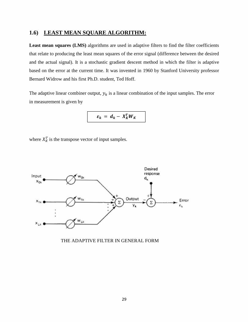
1.6) LEAST MEAN SQUARE ALGORITHM:

Least mean squares (LMS) algorithms are used in adaptive filters to find the filter coefficients

that relate to producing the least mean squares of the error signal (difference between the desired

and the actual signal). It is a stochastic gradient descent method in which the filter is adaptive

based on the error at the current time. It was invented in 1960 by Stanford University professor

Bernard Widrow and his first Ph.D. student, Ted Hoff.

The adaptive linear combiner output, is a linear combination of the input samples. The error

in measurement is given by

where is the transpose vector of input samples.

THE ADAPTIVE FILTER IN GENERAL FORM

http://en.wikipedia.org/wiki/1960

30

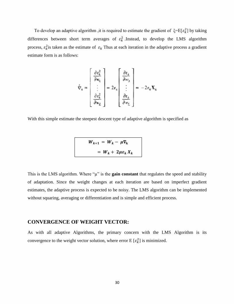
To develop an adaptive algorithm ,it is required to estimate the gradient of ξ=E[ ] by taking

differences between short term averages of .Instead, to develop the LMS algorithm

process, is taken as the estimate of Thus at each iteration in the adaptive process a gradient

estimate form is as follows:

With this simple estimate the steepest descent type of adaptive algorithm is specified as

This is the LMS algorithm. Where “µ” is the gain constant that regulates the speed and stability

of adaptation. Since the weight changes at each iteration are based on imperfect gradient

estimates, the adaptive process is expected to be noisy. The LMS algorithm can be implemented

without squaring, averaging or differentiation and is simple and efficient process.

CONVERGENCE OF WEIGHT VECTOR:

As with all adaptive Algorithms, the primary concern with the LMS Algorithm is its

convergence to the weight vector solution, where error E [ ] is minimized.

31

1.7) INCREMENTAL ADAPTIVE STRATEGIES OVER DISTRIBUTED

NETWORKS

Distributed processing deals with the extraction of information from data collected at nodes that

are distributed over a geographic area. For example, each node in a network of nodes could

collect noisy observations related to a certain parameter or phenomenon of interest. The nodes

would then interact with their neighbours in a certain manner, as dictated by the network

topology, in order to arrive at an estimate of the parameter or phenomenon of interest. The

objective is to arrive at an estimate that is as accurate as the one that would be obtained if each

node had access to the information across the entire network. In comparison, in a traditional

centralized solution, the nodes in the network would collect observations and send them to a

central location for processing. The central processor would then perform the required estimation

tasks and broadcast the result back to the individual nodes. This mode of operation requires a

powerful central processor, in addition to extensive amounts of communication between the nodes

and the processor. In the distributed solution, the nodes rely solely on their local data and on

interactions with their immediate neighbours. The amount of processing and communications is

significantly reduced.

32

The effectiveness of any distributed implementation will depend on the modes of cooperation that

are allowed among the nodes. Three such modes of cooperation are as follows:

(a) Incremental

(b) Diffusion

(c) Probabilistic diffusion.

In an incremental mode of cooperation, information flows in a sequential manner from one

node to the adjacent node. This mode of operation requires a cyclic pattern of collaboration

among the nodes, and it tends to require the least amount of communications and power. In a

diffusion implementation, on the other hand, each node communicates with all its neighbours as

dictated by the network topology .The amount of communication in this case is higher than in

an incremental solution. Nevertheless, the nodes have access to more data from their neighbours.

The communications in the diffusion implementation can be reduced by allowing each node to

communicate only with a subset of its neighbours. The choice of which subset of neighbours to

communicate with can be randomized according to some performance criterion.

The need for adaptive implementations, real-time operation, and low computational and

communications complexity, a distributed least-mean-squares (LMS)-like algorithm that

requires less complexity for both communications and computations and inherits the

robustness of LMS implementations. The proposed solution promptly responds to new data, as

the information flows through the network. It does not require intermediate averaging as in

consensus implementations; it neither requires two separate time scales.The distributed adaptive

solution is an extension of adaptive filters and can be implemented without requiring any direct

knowledge of data statistics; in other words, it is model independent.

33

1.8) SYSTEM IDENTIFICATION:

System identification is a general term to describe mathematical tools and algorithms that build

dynamical models from measured data. A dynamical mathematical model in this context is a

mathematical description of the dynamic behaviour of a system or process in either the time or

frequency domain. Examples include:

physical processes such as the movement of a falling body under the influence of gravity;

economic processes such as stock markets that react to external influences.

One could build a so-called white-box model based on first principles, process but in many cases

such models will be overly complex and possibly even impossible to obtain in reasonable time

due to the complex nature of many systems and processes. A much more common approach is

therefore to start from measurements of the behaviour of the system and the external influences

(inputs to the system) and try to determine a mathematical relation between them without going

into the details of what is actually happening inside the system. This approach is called System

Identification. Two types of models are common in the field of system identification:

Grey box model: Although the peculiarities of what is going on inside the system are not

entirely known, a certain model based on both insight into the system and experimental

data is constructed. This model does however still have a number of unknown free

parameters which can be estimated using system identification. Grey box modeling is

also known as semi-physical modeling.

Black box model: No prior model is available. Most system identification algorithms are

of this type.

FIGURE: SYSTEM IDENTIFICATION USING ADAPTIVE FILTER

http://en.wikipedia.org/wiki/Mathematical_model

http://en.wikipedia.org/wiki/System

http://en.wikipedia.org/wiki/Physical_system

http://en.wikipedia.org/wiki/Gravity

http://en.wikipedia.org/wiki/Economic_system

http://en.wikipedia.org/wiki/Stock_market

http://en.wikipedia.org/wiki/White-box

http://en.wikipedia.org/wiki/Parameter

http://en.wikipedia.org/wiki/Image:Lms_filter.png

34

1.9) HAMMERSTEIN MODEL:

Hammerstein models are composed of a static nonlinear gain and a linear dynamics part. In

some situations, they may be a good approximation for nonlinear plants. It has been approached

following two major directions. The first one consists in supposing a polynomial (or polygonal)

as the nonlinear element of the model. Then, the identification problem turns out to be a

parametric one since it consists in estimating the parameters of the model linear and nonlinear

parts. Parameter estimation is generally performed, based on adequate (known) structures of the

model. The second direction, commonly referred-to nonparametric, considers that the nonlinear

element of the model is not necessarily polynomial. It may be any continuous function.

However, even in this case the identification process involves a truncated series approximation

either of the nonlinear element or of related functions. Due to these finite series approximations,

the identification problem amounts, just as in the parametric approaches, to estimating a finite

number of parameters. The nonparametric methods usually involve probabilistic tools in the

estimation process of the unknown parameters. The convergence of the parameter estimates has

been analyzed, using stochastic tools, both for parametric and nonparametric methods. It is

shown that consistency can be achieved, with a parametric instrumental variable method, using

as input a strictly persistently exciting sequence or a white noise. Specific random inputs have

been used in nonparametric methods to ensure consistency and other properties.

It appears that both parametric and nonparametric approaches involve, explicitly or implicitly,

orthogonal function series approximations of the nonlinear element. This is a normal

consequence of the fact that the plant nonlinear element is characterized by a continuous function

F (v), defined on some real interval (say [vmin, vmax]), while the plant input sequence (say

{v(t)}) is a discrete-time sequence (i.e. t=0, 1, 2, …). Actually, a continuous real function F(.),

which is defined by an uncountable number of values F(v) (vmin v vmax), cannot be captured,

except for particular cases, by a countable set of values, namely {v(t); t=0, 1, …}.

A parametric identification scheme is designed to deal with the case where the static gain is any

(non-identically null) nonlinear function F.The proposed scheme identifies perfectly the model of

the plant dynamics and a set of N points ( ,F( )) (i=1, …, N) of the static gain characteristic

F,where N and the ‟s are chosen arbitrarily.

35

The points ( ,F( )) uniquely determine an Nth-degree polynomial P(v) that coincides with

F(v) on the ‟s, then identifying the points ( , F( )) amounts to identifying P(v). Furthermore,

letting the plant input be chosen in the set { , i=1… N}, allows substitution of P(v) to F(v) in

the plant model; so doing, the initial identification problem is converted to one where the

nonlinear element is polynomial. The mentioned substitution leads to a plant representation that

is linear in the unknown parameters. It is worth noting, that the involved parameters are bilinear

functions of the desired (unknown) parameters i.e. those of the plant dynamics, on one hand, and

those of the static gain, on the other hand.

Finally, a persistently exciting input sequence is designed and shown to guarantee the

convergence of the estimates to their true values. The proposed exciting input is an impulse type

sequence.

w(k)

u(k) x(k) t(k)

y(k)

The Hammerstein model structure

The Hammerstein systems are proved to be good descriptions of nonlinear dynamic systems in

which the nonlinear static subsystems and linear dynamic subsystems are separated in different

order. When the nonlinear element precedes the linear block, it is called the Hammerstein model

as shown in figure above.

The Hammerstein model is represented by the following equations:

STATIC

NONLINEARITY

LINEAR

DYNAMICS ∑

36

HAMMERSTEIN MODEL

U(k)

X(k)

0.7

V(k) y(k)

0.9

1.5

W(k)

0.15

1

0.02

0.41`

∑

X

X

∑ ∑ ∑

X

X

Z-1

Z-1

∑

Z-1

X

∑

Z-1

X

Z-1

Z-1

Z-1

∑

37

CHAPTER 2

38

AIM OF THE PROJECT

Our objective is therefore to study and analyse the various forms of Genetic algorithms and

their application to the problems of Function Optimisation and System Identification. Since there

are other methods traditionally adopted to obtain the optimum value of a function (which are

usually derivative based), the project aims at establishing the superiority of Genetic

Algorithms in optimizing complex, multivariable and multimodal functions.

1. The Genetic Algorithms need to be implemented to simple unimodal function optimization

like sine x.

2. Then the process is to be extended to complex multimodal functions like schwefel‟s

function.

3. The different forms of GA are to be comparatively studied analyzing their benefits in detail.

4. Then the Algorithm has to be extended to the System Identification problem and compared

with the incremental LMS algorithm.

39

CHAPTER 3

40

IMPLEMENTATION AND SIMULATION:

3.1) FUNCTION OPTIMISATION USING REA L CODED GENETIC

ALGORITHM:

FLOWCHART

START

DEFINE PROBABILITY OF CROSSOVER (p), PROBABILITY OF

MUTATION (q), CONSTANTS (α AND β)

GENERATE THE INITIAL POPULATION IN THE SEARCH SPACE.

A FEW INDIVIDUALS WERE MUTATED TO GENERATE THE

MUTATED CHILD POPULATION.

A CERTAIN NO. OF INDIVIDUALS WERE SELECTED FOR

CROSSOVER AND THE CHILD POPULATION WERE GENERATED

EVALUATE THE FITNESS OF EACH INDIVIDUAL USING THE

FITNESS FUNCTION (SINX) AND SORT IN DESCENDING ORDER.

THE INITIAL POPULATION,CHILD POPULATION AND MUTATED

POPULATION FORMED THE TOTAL POPULATION. EVALUATE

THE FITNESS FUNCTION AND SORT IN DESCENDING ORDER.

THE POPULATION OBTAINED IS THE OPTIMAL SOLUTION.

TERMINATION

CONDITION

SELECT THE BEST FIT INDIVIDUAL TO FORM THE ELITIST INDIVIDUAL

WHICH ACT AS THE POPULATION FOR NEXT GENERATION.

STOP

YES

NO

41

Algorithm for Function Optimisation using Real Coded GA:

STEP1: The parameters like Probability of Crossover (p), Probability of Mutation (q) are

defined. The constants α AND β are also defined.

STEP 2: A set of possible solutions called the “initial Population” is initialized such that the

values range uniformly throughout the search space. The size of the population is assumed to be

“n”

STEP3: The Fitness Value was calculated for each of the individuals and the population is sorted

in the decreasing order of the fitness. The fitness function used here is “sine” function.

STEP4: Using the “Roulette Wheel” method of selection, few individuals are selected to undergo

crossover.

STEP5: The crossover between two individuals produced two child

chromosomes. The child population is given by the formula

Where , are the qth and rth individuals of the parent population set.

is the crossing vector. Given by the formula:

is a normally distributed random number that determines the amount of gene

crossing.

is the gene selection vector and the crossover takes place when the value is 1

42

α (0<α<=1) is the crossover range that defines the evolutionary step size and is

equivalent to the step size in he LMS algorithm.

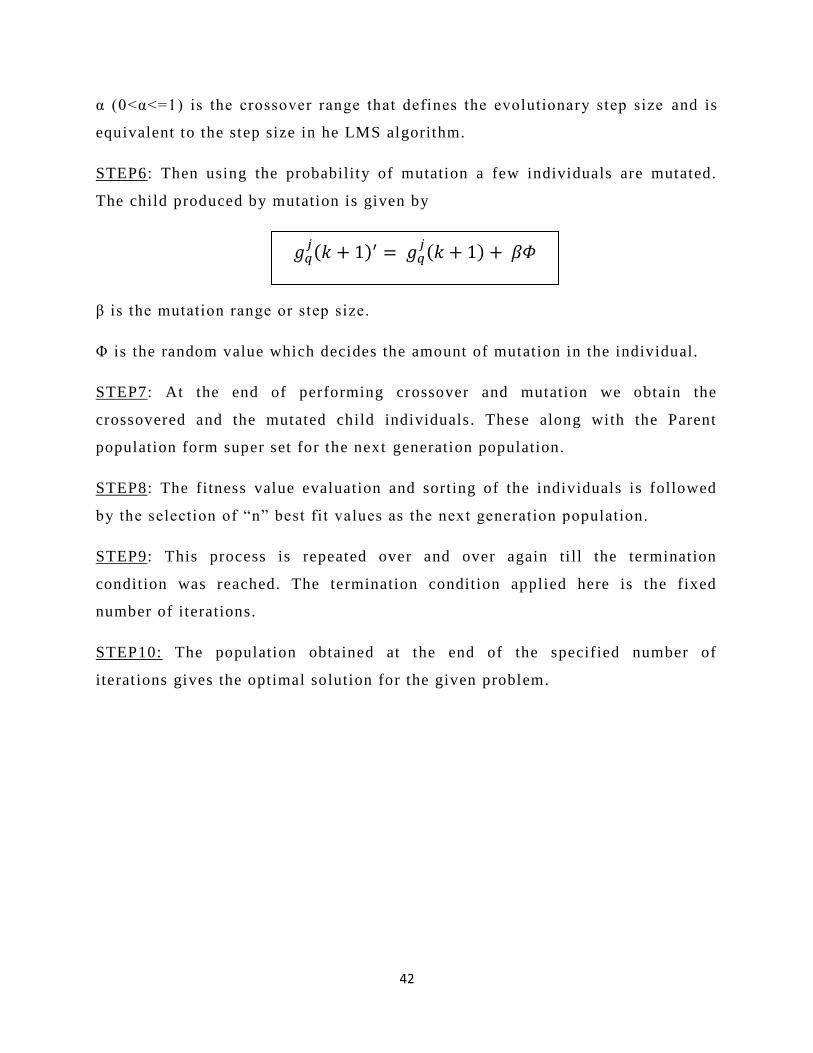
STEP6: Then using the probability of mutation a few individuals are mutated.

The child produced by mutation is given by

β is the mutation range or step size.

Φ is the random value which decides the amount of mutation in the individual.

STEP7: At the end of performing crossover and mutation we obtain the

crossovered and the mutated child individuals. These along with the Parent

population form super set for the next generation population.

STEP8: The fitness value evaluation and sorting of the individuals is followed

by the selection of “n” best fit values as the next generation population.

STEP9: This process is repeated over and over again ti ll the termination

condition was reached. The termination condition applied here is the fixed

number of iterations.

STEP10: The population obtained at the end of the specified number of

iterations gives the optimal solution for the given problem.

43

SIMULATION:

Fitness function: sine x

Probability of crossover (p) =0.8

Probability of mutation (q) = 0.2

Alpha = 0.2

Beta = 0.2

Initial population size = 20

No of iterations = 50

SIMULATION RESULTS:

PLOT OF FITNESS VERSUS ITERATIONS IN SINE X OPTIMISATION

USING REAL CODED GENETIC ALGORITHM

44

DISCUSSION:

The computation time for the above program was 0.06 seconds. It can be observed from the plot

that the value of the fitness converges to he optimal value in about 8-10 iterations. This

resembles a fairly good result in the optimization process.

45

3.2) FUNCTION OPTIMISATION USING SINGLE POINT CROSSOVER

BINARY GENETIC ALGORITHM:

FLOWCHART

START

DEFINE PROBABILITY OF CROSSOVER (p), PROBABILITY OF MUTATION (q)

GENERATE THE INITIAL POPULATION IN THE SEARCH SPACE AND REPRESENT

EACH INDIVIDUAL IN STRINGS OF 0‟S AND 1‟S(BINARY ENCODING)

A FEW INDIVIDUAL WERE MUTATED TO GENERATE THE

MUTATED POPULATION.

A CERTAIN NO. OF INDIVIDUAL WERE SELECTED FOR CROSSOVER AND THE

CHILD POPULATION WERE GENERATED USING SINGLE POINT CROSSOVER.

EVALUATE THE FITNESS OF EACH INDIVIDUAL FROM THE



POPULATION FORMED THE TOTAL POPULATION. EVALUATE

THE FITNESS FUNCTION AND SORT IN DESCENDING ORDER.


TERMINATION

CONDITION



STOP

YES

NO

-

+++

+

46

Algorithm for Function Optimization using Binary coded

GA(Single Point Crossover Method):

STEP1: The parameters like Probability of Crossover(p), Probability of Mutation(q) are defined.


values range uniformly throughout the search space. The size of the population was assumed to

be “n”. Each of the individual are called chromosomes and are in the form of string of 0‟s and

1‟s. Each bit in the chromosome is called a gene.

STEP3: The Fitness Value is calculated for each of the individuals and the population is sorted in

the decreasing order of the fitness. The fitness function used here is the “sine” function.


crossover.


chromosomes. The point of crossover is generated randomly for each set of

parents. And the genes after the crossover point are exchanged between the two

parent chromosomes to give the child chromosomes which contain the attributes

of both the parents.

STEP6: Then using the probability of mutation a few individuals are mutated. In

the process of mutation a bit is randomly chosen from the parent and the bit

value is reversed to obtain the mutated chromosome.


crossovered and the mutated child individuals. These along wit h the Parent

population forms the super set for the next generation population.




condition is reached. The termination condition applied here is the fixed number

of i terations.

47



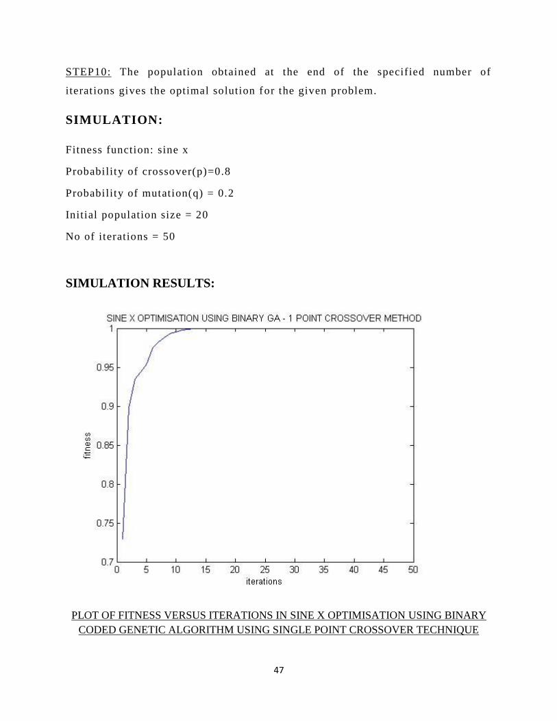
SIMULATION:


Probability of crossover(p)=0.8

Probability of mutation(q) = 0.2



SIMULATION RESULTS:

PLOT OF FITNESS VERSUS ITERATIONS IN SINE X OPTIMISATION USING BINARY

CODED GENETIC ALGORITHM USING SINGLE POINT CROSSOVER TECHNIQUE

48

DISCUSSION:

The computation time for the above program was 0.26 seconds. The computation time is more

from the real GA because of the need of converting data from real to binary form and vice versa.

It can be observed from the plot that the value of the fitness converges to the optimal value in

about 12-15 iterations. This resembles a fairly good result in the optimization process.

49

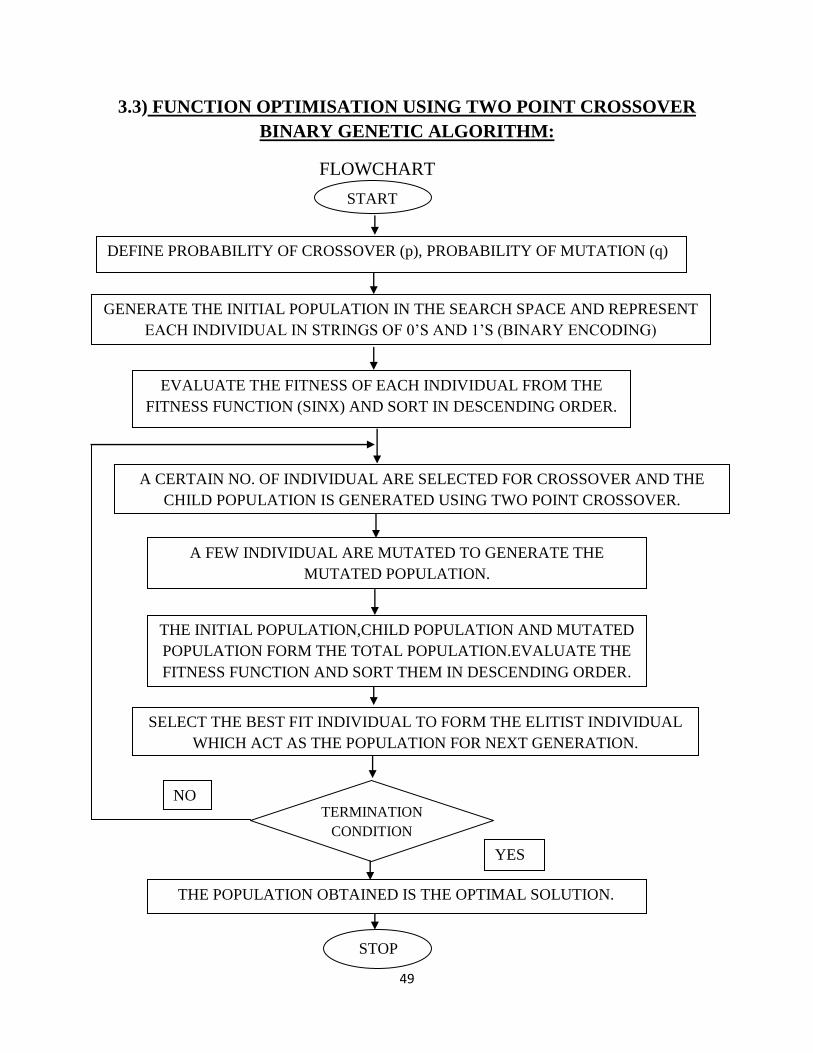
3.3) FUNCTION OPTIMISATION USING TWO POINT CROSSOVER

BINARY GENETIC ALGORITHM:

FLOWCHART

START

DEFINE PROBABILITY OF CROSSOVER (p), PROBABILITY OF MUTATION (q)

NO

YES




STOP

TERMINATION

CONDITION


POPULATION FORM THE TOTAL POPULATION.EVALUATE THE

FITNESS FUNCTION AND SORT THEM IN DESCENDING ORDER.

A FEW INDIVIDUAL ARE MUTATED TO GENERATE THE

MUTATED POPULATION.




EACH INDIVIDUAL IN STRINGS OF 0‟S AND 1‟S (BINARY ENCODING)

A CERTAIN NO. OF INDIVIDUAL ARE SELECTED FOR CROSSOVER AND THE

CHILD POPULATION IS GENERATED USING TWO POINT CROSSOVER.

50

Algorithm for Function Optimization using Binary coded GA (Two

Point Crossover Method):

STEP1: The parameters like Probability of Crossover (p), Probability of Mutation(q) are defined.






the decreasing order of the fitness. The fitness function used here is the “sine” function.


crossover.


chromosomes. The crossover is done by the exchange of genes between the two

parents. The gene information to be exchanged is the bits in between the two

crossover points. The points of crossover are generated randomly for each set of

parents. And the genes between the crossover points are exchanged between the

two parent chromosomes to give the child chromosomes which contain the

attributes of both the parents.









51



of i terations.

STEP10: The populat ion obtained at the end of the specified number of


SIMULATION:






SIMULATION RESULTS:

PLOT OF FITNESS VERSUS ITERATIONS IN SINE X OPTIMISATION USING BINARY

CODED GENETIC ALGORITHM USING TWO POINT CROSSOVER TECHNIQUE

52

DISCUSSION:

The computation time for the above program was 0.28 seconds. The computation time is more

from the real GA because of the need of converting data from real to binary form and vice versa.

But is nearly same as that of the single point crossover binary GA because both involve equal

number of computations.

It can be observed from the plot that the value of the fitness converges to the optimal value in

about 8-10 iterations. This resembles a better result in the optimization process than the single

point crossover technique where the convergence occurs after around 15 iterations.

53

3.4) FUNCTION OPTIMISATION USING SAWTOOTH GENETIC

ALGORITHM:

FLOWCHART

START

DEFINE PROBABILITY OF CROSSOVER (p), PROBABILITY OF MUTATION (q),

REINITIALISATION PERIOD (T), REINITIALISATION AMPLITUDE (D)

NO

YES


SELECT THE BEST FIT INDIVIDUAL TO FORM THE ELITIST INDIVIDUAL. A

FIXED NO („D‟) IS DECREASED FROM THE ELITIST POPULATION TO FORM THE

POPULATION FOR THE NEXT GENRATION.

STOP

TERMINATION

CONDITION


FITNESS FUNCTION AND SORT IN DESCENDING ORDER.

GENERATE THE INITIAL POPULATION („N‟) IN THE SEARCH SPACE AND REPRESENT


A CERTAIN NO. OF INDIVIDUAL ARE SELECTED FOR CROSSOVER AND THE CHILD

POPULATION IS GENERATED. A FEW INDIVIDUAL ARE MUTATED TO GENERATE THE

MUTATED POPULATION. THE INITIAL POPULATION, CHILD POPULATION AND

MUTATED POPULATION FORM THE TOTAL POPULATION. EVALUATE THE FITNESS

FUNCTION AND SORT THEM IN DESCENDING ORDER.

REINITIALISATION

CONTIDION REACHED

YES

REINITIALISE THE

POPULATION

NO

54

Algorithm for Function Optimisation using Sawtooth GA

STEP1: The parameters like Probability of Crossover(p), Probability of Mutation(q) are defined.

The Period of Reinitialisation(T) and the Amplitude of Reinitialisation are defined.






the decreasing order of the fitness.


crossover.


chromosomes. The point of crossover is generated randomly for each set of

parents. And the genes after the crossover point are exchanged between the two

parent chromosomes to give the child chromosomes which contain the attributes

of both the parents.







STEP8: The fitness value evaluation and sorting of the indiv iduals is followed

by the selection of “n -D” best fit values as the next generation population. So at

each generation the population size is decreased by the amplitude.

STEP9: This process is repeated over and over again t ill the periodicity of

reinitialisation is reached.

55

STEP10: A set of randomly generated individuals are reinitialized into the

parent population set and the process is started all over again through selection,

crossover and mutation.

STEP11: This stops when the termination condition is reached which here is the

fixed number of iterations.



SIMULATION 1(Unimodal Function):


Probability of crossover (p)=0.8




Period of Reinitialisation = 2

Amplitude of Reinitialisation = 10

56

SIMULATION RESULT:


USING SAWTOOTH GENETIC ALGORITHM

SIMULATION 2(Multivariable Function)

Fitness function: Rosenbrock‟s Function





Period of Reinitialisation =20


57

ROSENBROCK FUNCTION:

In mathematical optimization, the Rosenbrock function is a non-convex function used as a test

problem for optimization algorithms. It is also known as Rosenbrock's valley or Rosenbrock's

banana function. This function is often used to test performance of optimization algorithms.

The global minimum is inside a long, narrow, parabolic shaped flat valley. To find the valley is

trivial, however to converge to the global minimum is difficult. It is defined by

It has a global minimum at (x,y) = (1,1) where f(x,y) = 0. A common multidimensional extension

For [0,2] min f = 0 with = 1, i=1,2,3…N

N = no of variables = 3

PLOT FOR ROSENBROCK FUNCTION

http://en.wikipedia.org/wiki/Convex_function

58

SIMULATION RESULT

i) USING REAL SAWTOOTH GA

PLOT OF FITNESS VERSUS ITERATIONS IN ROSENBROCK FUNCTION

OPTIMISATION USING REAL SAWTOOTH GENETIC ALGORITHM

59

ii) USING BINARY SAWTOOTH GA

PLOT OF FITNESS VERSUS ITERATIONS IN ROSENBROCK

FUNCTION OPTIMISATION USING BINARY SAWTOOTH

GENETIC ALGORITHM

SIMULATION 3 (Multimodal Function)

Fitness function: Scwefel Function

Probability of crossover (p)=0.8




Period of Reinitialisation =16


60

SCWEFEL FUNCTION:

Schwefel's function is deceptive in that the global minimum is geometrically distant, over the

parameter space, from the next best local minima. Therefore, the search algorithms are

potentially prone to convergence in the wrong direction.

The function definition:

global minimum of f(x) is

f(x)= - 416.99N ; =416.99 , i=1:N. Here N=10

PLOT FOR SCHWEFEL FUNCTION

61

SIMULATION RESULT:

PLOT OF FITNESS VERSUS ITERATIONS IN SCHWEFEL

FUNCTION OPTIMISATION USING BINARY SAWTOOTH

GENETIC ALGORITHM

DISCUSSION:

The computation times for the above programs are

Unimodal - 0.14 seconds.

Rosenbrock real coded- 1.36 seconds

Rosenbrock binary coded-19.7 seconds

Schwefel - 55 seconds

62

The computation time is more from the real coded rosenbrock optimization than

that of binary coded because of the need of converting data from real to binary

form and vice versa.

It can be observed from the plot that the saw tooth GA gives a precise convergence

of the function in both unimodal and multimodal functions.

63

3.5) FUNCTION OPTIMISATION USING DIFFERENTIAL EVOLUTION

GENETIC ALGORITHM:

FLOWCHART

START

DEFINE PROBABILITY OF CROSSOVER (cr), CONSTANT F (0<F<2)



NO

YES


STOP

TERMINATION

CONDITION

THE PERTURBED VECTOR IS GENERATED BY RANDOMLY CHOSING ANY THREE

INDIVIDUALS FROM THE INTIAL POPOULATION AND ADDING THE WEIGHTED

DIFFERENCE OF TWO OF THEM TO THE THIRD.

DURING CROSSOVER, THE STARTING POINT (n)AND NO. OF BITS(L) TO BE

EXCHANGED IS DETERMINED.

THE CHILD POPULATION IS GENERATED BY COPYING THE BITS FROM

PERTURBED VECTOR ACCORDING TO „n „AND „L‟ AND REST BITS FROM PARENT

POPULATION.

THE FITNESS VALUE OF THE PARENT POPULATION AND CHILD POPULATION

FROM THE FITNESS FUNCTION ARE EVALUATED.

SELECT THE BEST FIT INDIVIDUAL BETWEEN PARENT AND CHILD POPULATION

ACCORDING TO THEIR FITNESS VALUE TO FORM THE POPULATION OF NEXT

GENERATION .

64

Algorithm for Function Optimization using Differential Evolution

GA:

STEP1: The parameters like Probability of Crossover (Cr), weight of differential addition F are

defined.



be “NP”. Each of the individual are called chromosomes and are in the form of string of 0‟s and


STEP3: A perturbed vector is generated for each parent chromosome using the formula

Where i, r1, r2, r3 are all integers [1, NP] and are mutually different from one another.

STEP4: Crossover operator is applied between the perturbed vector and its corresponding parent vector.

The point of crossover is randomly selected between 0 – D-1, where D is the bit length of each

chromosome. The number of bits to be exchanged is determined by the algorithm

STEP5: The crossover produces a child chromosome. Using the formula

L = 0;

do {

L = L + l ;

}while(rand()< CR) AND (L < D ) ) ;

,

=

65

Where v is the perturbed vector and u is the crossovered child.

< > implies the modulo function

STEP6: The fitness value of the Parent and the child is evaluated and the better

fit of he two is selected as the next generation population.



of i terations.

STEP8: The population obtained at the end of the specified number of iterations

gives the optimal solution for the given problem.

SIMULATION:

Fitness function: sine x, x^2 and sphere function

Probability of crossover(Cr)=0.8


SPHERE FUNCTION is given by

For x(-200,200) the min value of the function is 0 at the points = 0

66

SIMULATION RESULTS:


USING DIFFERENTIAL EVOLUTION GENETIC ALGORITHM

67

PLOT OF FITNESS VERSUS ITERATIONS IN X2 OPTIMISATION USING

DIFFERENTIAL EVOLUTION GENETIC ALGORITHM

68

PLOT OF FITNESS VERSUS ITERATIONS IN SPHERE FUNCTION

OPTIMISATION USING DIFFERENTIAL EVOLUTION GENETIC

ALGORITHM

DISCUSSION:

The computation of the 1000 iterations in sin x optimization takes 7.29 seconds. It

can be observed from the plots that the value of the fitness converges to the

optimal value in both single variable and multi variable problems. But in case of a

multi variable function the convergence takes a little longer which is due to the

increase in the no of variables to be optimized.

69

3.6) SYSTEM IDENTIFICATION USING LMS:

FLOWCHART:

START

INITIALISE THE NO. OF INPUTS, GAIN CONSTANT AND

FILTER PARAMETERS OF KNOWN SYSTEM.

TEMPORARY STORAGE OF FILTER

PARAMETERS OF UNKNOWN SYSTEM.

ESTIMATED FINAL PARAMTERS OF UNKNOWN SYSTEM.

CALCULATION OF THE DESIRED AND ESTIMATED

OUTPUT USING FILTER PARAMETERS OF UNKNOWN

AND KNOWN SYSYSTEM.

CALCULATION OF

THE ERROR.

TERMINATION

CONDITION

STOP

UPDATE THE FILTER PARAMETERS USING THE ERROR

AND GAIN CONSTANT AND CURRENT SET OF INPUTS.

NO

YES

70

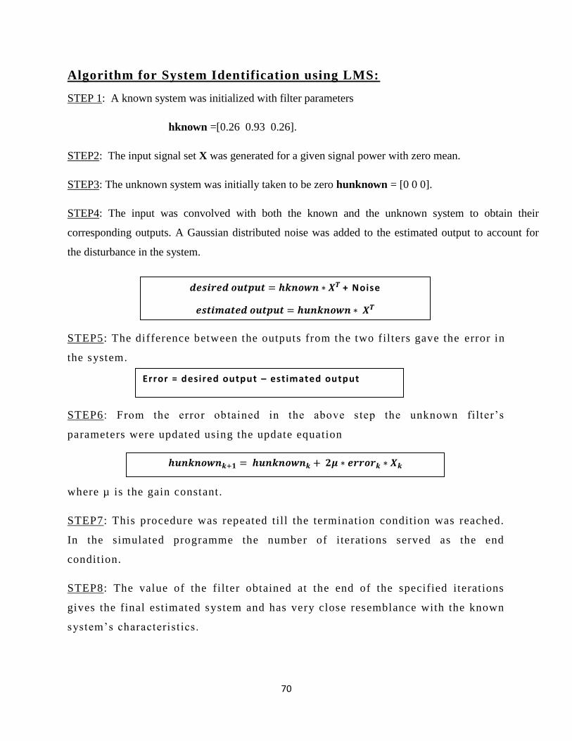
Algorithm for System Identification using LMS:

STEP 1: A known system was initialized with filter parameters

hknown =[0.26 0.93 0.26].

STEP2: The input signal set X was generated for a given signal power with zero mean.

STEP3: The unknown system was initially taken to be zero hunknown = [0 0 0].

STEP4: The input was convolved with both the known and the unknown system to obtain their

corresponding outputs. A Gaussian distributed noise was added to the estimated output to account for

the disturbance in the system.

STEP5: The difference between the outputs from the two filters gave the error in

the system.

STEP6 : From the error obtained in the above step the unknown filter‟s

parameters were updated using the update equation

where µ is the gain constant.

STEP7: This procedure was repeated till the termination condition was reached.

In the simulated programme the number of iterations served as the end

condition.

STEP8: The value of the filter obtained at the end of the specified iterations

gives the final estimated system and has very close resemblance with the known

system‟s characterist ics.

+ Noise

Error = desired output – estimated output

71

STEP9: A graph was plotted between error square and the no of i terations to

show the convergence. When error tends to zero the system is said to have

converged with the known sys tem. Hence the system is identified.

SIMULATION RESULTS:

PLOT OF ERROR SQUARE VERSUS NO OF ITERATIONS IN A SYSTEM

IDENTIFICATION PROCESS IMPLEMENTING LMS ALGORITHM

72

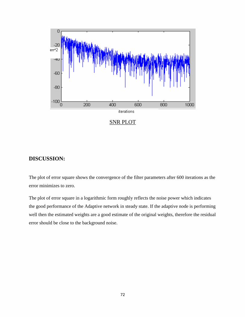
SNR PLOT

DISCUSSION:

The plot of error square shows the convergence of the filter parameters after 600 iterations as the

error minimizes to zero.

The plot of error square in a logarithmic form roughly reflects the noise power which indicates

the good performance of the Adaptive network in steady state. If the adaptive node is performing

well then the estimated weights are a good estimate of the original weights, therefore the residual

error should be close to the background noise.

73

3.7) SYSTEM IDENTIFICATION USING INCREMENTAL APPROACH

(Random Input):

FLOWCHART:

START

INITIALISE NO. OF NODES IN THE SYSTEM (N), NO. OF INPUTS, GAIN

CONSTANT AND THE FILTER PARAMETERS OF NODES OF KNOWN

SYSTEM.

N=1 N=N+1

N<=NO OF SENSORS

CALCULATION OF THE DESIRED OUTPUT AND ESTIMATED OUTPUT

AT A PARTICULAR NODE.

CALCULATION OF ERROR AT THAT NODE.

UPDATE THE FILTER PARAMETERS USING THIS ERROR, CURRENT SET OF INPUT AND

GAIN CONSTANT AND PASS THESE FILTER PARAMETERS TO NEXT NODE

CYCLICALLY.

TERMINATION

CONDITION

TEMPORARY STORAGE OF FILTER PARAMETERS OF THE NODES OF

UNKNOWN SYSTEM.

ESTIMATED FINAL PARAMETERS OF EACH NODE OF THE

UNKNOWN SYTEM.

STOP

NO

YES

YES

NO

74

COMPARATIVE ANALYSIS OF CENTRALISED AND INCREMENTAL

APPROACH ALGORITHMS:

STEP 1: A known system of a few sensors was initialized with predefined filter parameters.

STEP 2: Input signal set X was generated for a given signal power with zero Mean.

STEP3: The parameters at the sensors were initially taken to be zero.

hunknown = [0 0 0] for each of the sensors.

STEP 4: The input was convolved with both the known and the unknown system at the first sensor to

obtain their corresponding outputs. A Gaussian distributed noise was added to the estimated output to

account for the disturbance in the system.

STEP 5: The difference between the outputs from the two fil ters gave the error

in the system.

.

STEP 6: From the error obtained in the above step the unknown fi lter‟s

parameters were updated using the update equation.

where μ is the gain constant.

STEP 7: The updated parameters from the first sensor were passed as initial

weights for the next sensor and the above processes were repeated.

STEP 8: Once we reached the last sensor the updated value of the fi lter

parameter from the last sensor is passed onto the first sensor and the process

was continued till we reached the termination condition.

+ Noise


75

STEP 9: The convergence of the INCREMENTAL LMS technique was compared

with that of a centralised LMS process where each sensor was treated as an

independent system identification problem.

STEP 10: A graph of error square versus no of i terations was plotted for both

the processes adopted and their convergence speed and efficiency were

compared .

SIMULATION RESULTS:

PLOT OF ERROR SQUARE vs NO OF ITERATIONS IN A CENTRALIZED

APPROACH

76

PLOT OF ERROR SQUARE vs NO OF ITERATIONS IN INCREMENTAL

APPROACH

DISCUSSION:

A Relative study of the two graphs clearly enforces the better efficiency of the incremental LMS

technique over the Centralized technique.

(a) In the plot for Centralized LMS the convergence occurs after over 600 iterations.

(b) In the plot for Incremental LMS the convergence is bit faster and is attained in about 200

iterations.

77

3.8) INCREMENTAL STRATEGIES OVER DISTRIBUTED SYSTEM:

INCREMENTAL ADAPTIVE STRATEGIES: It is a reflection of a result in optimization theory that the incremental strategy can outperform

the steepest-descent technique. Intuitively, this is because the incremental solution incorporates

local information on-the-fly into the operation of the algorithm, i.e., it exploits the spatial

diversity more fully. While the steepest-descent solution has fixed throughout all spatial

updates, the incremental solution uses instead the successive updates.

The network has N=20 nodes with unknown vector , M=10, and

relying on independent Gaussian regressors. The background noise is white and Gaussian. The

output data are related via

for each node. The curves are obtained by averaging over 300 iterations.

PERFORMANCE ANALYSIS: Studying the performance of such an interconnected network of nodes is challenging (more

so than studying the performance of a single LMS filter) for the following reasons:

1) Each node is influenced by local data with local statistics (spatial information);

2) Each node is influenced by its neighbours through the incremental mode of

cooperation(Spatial interaction);

3) Each node is subject to local noise with variance (spatial noise profile).

78

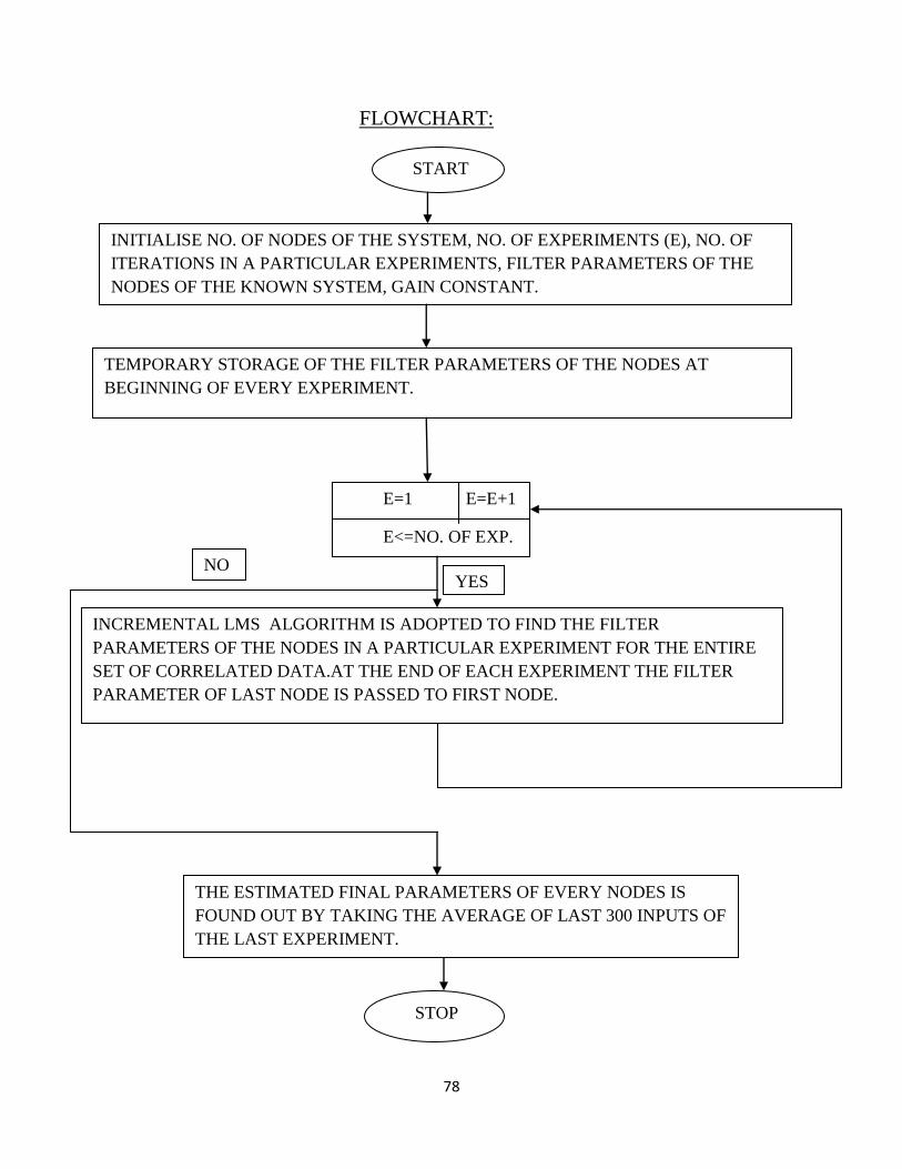
FLOWCHART:

START

INITIALISE NO. OF NODES OF THE SYSTEM, NO. OF EXPERIMENTS (E), NO. OF

ITERATIONS IN A PARTICULAR EXPERIMENTS, FILTER PARAMETERS OF THE

NODES OF THE KNOWN SYSTEM, GAIN CONSTANT.

TEMPORARY STORAGE OF THE FILTER PARAMETERS OF THE NODES AT

BEGINNING OF EVERY EXPERIMENT.

E=1 E=E+1

E<=NO. OF EXP.

INCREMENTAL LMS ALGORITHM IS ADOPTED TO FIND THE FILTER

PARAMETERS OF THE NODES IN A PARTICULAR EXPERIMENT FOR THE ENTIRE

SET OF CORRELATED DATA.AT THE END OF EACH EXPERIMENT THE FILTER

PARAMETER OF LAST NODE IS PASSED TO FIRST NODE.

STOP

THE ESTIMATED FINAL PARAMETERS OF EVERY NODES IS

FOUND OUT BY TAKING THE AVERAGE OF LAST 300 INPUTS OF

THE LAST EXPERIMENT.

YES NO

79

Algorithm:

STEP 1: The Network has 20 sensors pursuing the same unknown vector

With M = 10 that specifies the filter length.

STEP 2: Input signal set X was generated for each of the nodes from the given signal power

profile. The signal generated is a set of “Correlated Data”.

STEP3: The parameters at the sensors were initially taken to be zero.

hunknown = [0 0 0] for each of the sensors.

STEP 4: The input was convolved with both the known and the unknown system at the first sensor to

obtain their corresponding outputs.

A Gaussian distributed noise was added to the estimated output to account for the disturbance in the

system. The noise was obtained from the given signal to noise ratio for each node.

STEP 5: The difference between the outputs from the two fil ters gave the error

in the node.

.

STEP 6: From the error obtained in the above step the unknown fi lter‟s

parameters were updated using the update equation

where μ=0.03 is the gain constant.

+ Noise


80

STEP 7: The updated parameters from the first sensor were passed as initial

weights for the next sensor and the same above processes were repeated.

STEP 8: Once we reached the last sensor the updated value of the fi lter

parameter from the last sensor was passed onto the first sensor. This completed

one iteration of our operation.

STEP 9: At the end of the required no of iterations all the inputs have been

evaluated once at their respective sensors. This completes one Experiment .

STEP10: At the end of all the experiments the average weights of the last 300

iterations was obtained.

STEP 11: A graph of MSE(Mean Square Error), EMSE(Excess Mean Square

Error) and MSD(Mean Square Deviation) was plotted against each node.

81

SIMULATION RESULTS:

MEAN SQUARE DEVIATION ACROSS NODES

MEAN SQUARE ERROR ACROSS NODES

EXCESS MEAN SQUARE ERROR ACROSS NODE

82

Computer simulations were done in MATLAB environment to make a thorough study of the

performance of the Incremental type LMS Algorithm. In order to plot performance curves 100

different experiments were performed and the values of the last 300 iterations after the

convergence were averaged. The quantities of interest:

MSD(Mean Square Deviation)

MSE(Mean Square Error)

EMSE(Excess Mean Square Error) were obtained.

83

In the Simulation N=20 nodes were taken with each regressor size of (1X10) collecting data

from time correlated sequence { , generated as

i > -∞

is a spatially independent white Gaussian process with unit variance

The correlation indices and the Gaussian noise variances were chosen a random. The

corresponding Signal to Noise Ratio obtained at each node.

DISCUSSION:

The MSE roughly reflects the noise power which indicates the good performance of the Adaptive

distributed network in steady state. If the adaptive node is performing well then the estimated

weights are a good estimate of therefore the residual error should be close to the background

noise.

The graphs obtained for the MSE and EMSE were in close resemblance with the graphs obtained

in the IEEE paper “Incremental Adaptive Strategies over Distributed Networks” implemented by

Lopes and Sayed. There was some difference observed in the plot of MSD.

(i)

84

3.9) SYSTEM IDENTIFICATION USING GENETIC ALGORITHM:

FLOWCHART

START

COEFFICIENTS OF THE SYSTEM ARE INITIALLY CHOSEN TO FORM

POPULATION OF M-CHROMOSOMES

EACH CHROMOSOME CONSTITUTES NL NUMBER OF RANDOM BINARY BITS

WHERE EACH SEQUENTIAL GROUP OF LBITS L-BITS REPRESENT ONE

COEFFICIENT OF THE ADAPTIVE MODEL, WHERE N IS THE NUMBER OF

PARAMETERS OF THE MODEL.

.

EACH OF THE INPUT SAMPLE IS PASSED THROUGH THE PLANT AND THEN

CONTAMINATED WITH THE ADDITIVE NOISE OF KNOWN STRENGTH,

WHICH ACTS AS DESIRED SIGNAL (HAVING K SAMPLES).

SIMILARLY EACH SAMPLE IS ALSO PASSED THROUGH THE MODEL USING

EACH CHROMOSOME AS MODEL PARAMETERS & M-SETS OF K-ESTIMATED

OUTPUTS ARE OBTAINED.

EACH OF THE DESIRED OUTPUT IS COMPARED WITH CORRESPONDING

ESTIMATED OUTPUT AND K ERRORS ARE PRODUCED

.

FINALLY ALL THE CHROMOSOMES WILL ATTEND ALMOST IDENTICAL

GENES, WHICH REPRESENTS THE ESTIMATED PARAMETERS OF THE

DEVELOPED MODEL.

STOP

GENERATE K NUMBER OF INPUT SIGNAL SAMPLES.

MSE OF EACH CHROMOSOMES ARE OBTAINED WHICH ACT AS THE

COST FUNCTION WHICH IS MINIMISED BY GA.

OPERATORS OF GA ARE SEQUENTIALLY CARRIED OUT TO MINIMIZE MSE

85

Algorithm for System Identification using Genetic Algorithm:

STEP 1: A known plant was initialized with filter parameters

hknown =[0.26 0.93 0.26].

STEP2: The input signal set X was generated for a given signal power with unit amplitude.



corresponding outputs. A Gaussian distributed noise was added to the estimated output to account for

the disturbance in the system.


the system .

STEP6: The population is sorted on the basis of the mean square error

associated with it .

STEP7: The selected individuals undergo crossover and mutation to produce the

net generation population.

STEP8: This procedure is repeated till the termination condition is reached. In

the simulated programme the number of i terations served as the end condition.




+ Noise


86

STEP10: Different graphs are plotted to show the outputs of the known and the

unknown plant for a given set of inputs.

SIMULATION:



Alpha = 0.2

Beta = 0.2



No of inputs = 100

87

SIMULATION RESULT:

PLOT SHOWING THE OUTPUT OF THE KNOWN AND THE IDENTIFIED PLANT FOR

THE GIVEN SET OF INPUTS

DISCUSSION:

The system in the problem was perfectly identified with the mean square error

tending towards zero. This proves the efficiency of the GA in system identification

problem.

88

3.10) SYSTEM IDENTIFICATION USING DIFFERENTIAL EVOLUTION

GENETIC ALGORITHM:

FLOWCHART

START

COEFFICIENTS OF THE SYSTEM ARE INITIALLY CHOSEN TO FORM

POPULATION OF M-CHROMOSOMES

EACH CHROMOSOME CONSTITUTES NL NUMBER OF RANDOM BINARY BITS

WHERE EACH SEQUENTIAL GROUP OF LBITS L-BITS REPRESENT ONE

COEFFICIENT OF THE ADAPTIVE MODEL, WHERE N IS THE NUMBER OF

PARAMETERS OF THE MODEL.

.

EACH OF THE INPUT SAMPLE IS PASSED THROUGH THE PLANT , WHICH

ACTS AS DESIRED SIGNAL (HAVING K SAMPLES).

SIMILARLY EACH SAMPLE IS ALSO PASSED THROUGH THE MODEL USING

EACH CHROMOSOME AS MODEL PARAMETERS & M-SETS OF K-ESTIMATED

OUTPUTS ARE OBTAINED.

EACH OF THE DESIRED OUTPUT IS COMPARED WITH CORRESPONDING

ESTIMATED OUTPUT AND K ERRORS ARE PRODUCED

NNNNNNNNNNNNNNNNNNNNNNNNNNNNNNNNNNNNNNNNNNNNNNN




















FINALLY ALL THE CHROMOSOMES WILL ATTAIND ALMOST IDENTICAL

GENES, WHICH REPRESENTS THE ESTIMATED PARAMETERS OF THE

DEVELOPED MODEL.

STOP

GENERATE K NUMBER OF INPUT SIGNAL SAMPLES.

MSE OF EACH CHROMOSOMES ARE OBTAINED WHICH ACT AS THE

COST FUNCTION WHICH IS MINIMISED BY DE.

OPERATORS OF DE ARE SEQUENTIALLY CARRIED OUT TO MINIMIZE MSE

89

Algorithm for System Identification using LMS:

STEP 1: A known plant was initialized with filter parameters

hknown =[0.26 0.93 0.26].

STEP2: The input signal set X was generated for a given signal power with unit amplitude.



corresponding outputs.


the system .

STEP6: The population is sorted on the basis of the mean square error

associated with it .

STEP7: The selected individuals generate their respective perturbed vectors.

The parent chromosome is crossovered with the perturbed vector to form the

child. The child if fitt er replaces the parent individual else the parent

chromosome is retained in the next generation.

STEP8: This procedure is repeated till the termination condition is reached. In

the simulated programme the number of i terations served as the end condition.





90

STEP10: Different graphs are plotted to show the outputs of the known an d the

unknown plant for a given set of inputs.

SIMULATION:

Probability of crossover(Cr )=0.8



No of inputs = 100

SIMULATION RESULT:

PLOT SHOWING THE OUTPUT OF THE KNOWN AND THE IDENTIFIED

PLANT FOR THE GIVEN SET OF INPUTS

91

DISCUSSION:

The system in the problem was perfectly identified with the mean square error tending towards

zero. The application of Differential evolution algorithm to the system identification problem

shows closer approximation of the filter parameters.

The graph shows that the output of the estimated plant closely follows the output of the known

plant for the given set of inputs.

92

CHAPTER 4

93

4. CONCLUSION

The results obtained by simulation of the Function Approximation problem reveals the

superiority of the Genetic Algorithm over the other methods of optimization in both unimodal

and multimodal functions. The different algorithms of the real coded GA, binary coded GA,

Sawtooth GA and Differential Evolution GA have their own advantages and disadvantages in the

different optimization problems. Real coded GA has faster convergence than Binary GA. Further

Twp point crossover Binary GA is better than Single point crossover Binary GA because it

brings better randomness in the search space. Sawtooth GA worked efficiently for both unimodal

and multimodal function because of the variabile population factor. Differential Evolution (DE)

proves to be a promising candidate for optimizing real valued multi-modal objective functions.

The results obtained by simulation of the System Identification problem shows both Real coded

GA and Differential Evolution GA are effective tool to design the model which is the replica of

the system. The output produced by the known plant and the system model by Real Coded GA

and Differential Evolution GA perfectly matched.

System identification using LMS algorithm gives lesser error than in GA technique. But the

efficiency of LMS algorithm is restricted to linear systems and becomes unstable as the number

of parameter increases. The increase in he number of parameters also increases the

computational complexity in LMS but in GA there is very little increase in the computation.

Thus, this paper summarizes a number of current developments in genetic algorithms. It includes

both theoretical aspects of genetic algorithms and its variants and some potential applications

which incorporate the use of genetic algorithms.

94

5. REFERENCES

1) Phillip David Power, “Non Linear Multi Layer Perceptron Channel Equalisation”,Chapter 4

„Genetic Algorithm Optimisation‟, in IEEE Transactions,The Queen University of Belfast,April

2001.

2) Jacob D. Griesbach and Delores M. Etter,” Fitness-Based Exponential Probabilities for

Genetic Algorithms Applied to Adaptive IIR Filtering”, in IEEE Transactions, Department of

Electrical and Computer EngineeringUniversity of ColoradoBoulder.

3) Vlasis K. Koumousis and Christos P. Katsaras,” A Saw-Tooth Genetic Algorithm Combining

the Effects of Variable Population Size and Reinitialization to Enhance Performance”, IEEE

Transactions on Evolutionary Computation, Vol. 10, No. 1, February 2006.

4) Rainer Storn and Kenneth Price,” Minimizing the Real Functions of the ICEC'96 contest

by Differential Evolution” , in IEEE Transactions .

5) Uday K. Chakraborty ,Swagatam Das and Amit Konar,” Differential Evolution with Local

Neighborhood” in IEEE Congress on Evolutionary Computation Sheraton Vancouver Wall

Centre Hotel, Vancouver, BC, Canada, July 16-21, 2006

6) Zhixiang HOU,” Hammerstein Model Identification Based on Adaptive Particle Swarm

Optimization”, Workshop on Intelligent Information Technology Application, Changsha

University of Science and Technology Changsha, China, in IEEE Publications, 2007.

95

7) C.G.Lopes and A.H.Sayed, ”Incremental Adaptive Strategies Over Distributed Networks”

in IEEE Transactions on Signal Processing, Vol. 55, No 8, August 2007.

8) C.G.Lopes A.H.Sayed,”Distributed Adaptive Strategies: Formulation and Performace

Analysis”, in PROC. IEEE Int.Conf. Acoustics, Speech, Signal Processing, (ICASSP), Toulouse,

Vol 3. France , May 2006.

9) Bernard Widrow and Samauel D.Stearns, “Adaptive Signal Processing”. Pearson

Education,Second Impression,2009.

10) www.wikipedia.org.

genetic algorithm and its variants: theory and...

Documents