GENERALIZED FLOWS

Jonathan Kalechstain27.5.2013

Tel Aviv University

Introduction

• Until now, we made an assumption that if k units of flow leaves node u, then k units of flow arrives at node v.

• This assumption may not be always true, like in transmission of unstable gas , or leaking pipes.

uk

v

Using multipliers

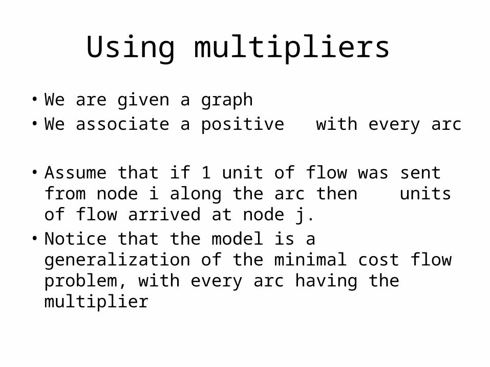
• We are given a graph • We associate a positive with every arc • Assume that if 1 unit of flow was sent from

node i along the arc then units of flow arrived at node j.

• Notice that the model is a generalization of the minimal cost flow problem, with every arc having the multiplier

Example

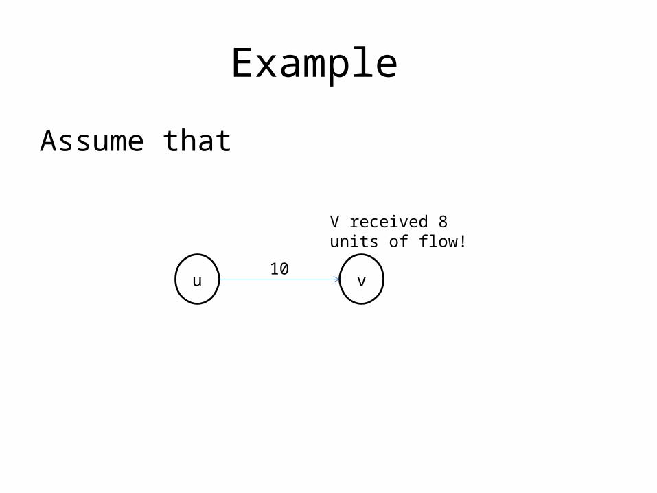
Assume that

u10

v

V received 8 units of flow!

Notations and Assumptions

• G=(V,E) is a directed graph• Capacity function u(v,w) > 0 for every • Cost function c(v,w) for every • An arc multiplier for every • Balance function b(v) for every we will have a

number– b(v) > 0 – supply– b(v) < 0 – demand

Formulation Of The Generalized Flow Problem(linear programming)

• Minimize Subject to:

And

An Important Remark

• is an upper bound on the flow that we send from i, not the flow that arrives at node j.

• is the cost per unit flow we send from i, not the per unit cost that arrives at node j

Example

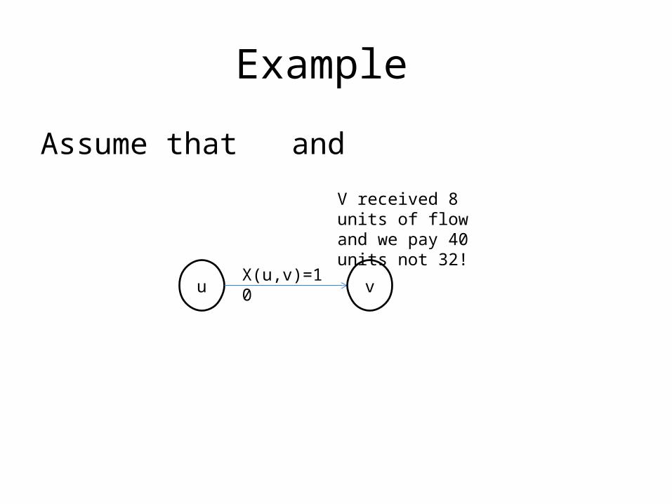
Assume that and

uX(u,v)=10

v

V received 8 units of flow and we pay 40 units not 32!

Augmented Forest structures

Flows along Paths

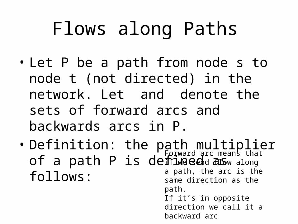
• Let P be a path from node s to node t (not directed) in the network. Let and denote the sets of forward arcs and backwards arcs in P.

• Definition: the path multiplier of a path P is defined as follows:

Forward arc means that if we send flow along a path, the arc is the same direction as the path.If it’s in opposite direction we call it a backward arc

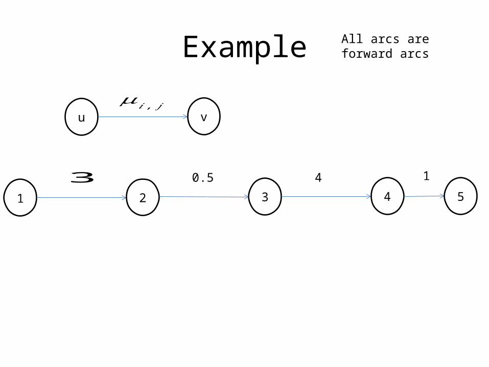
Example

u v𝜇𝑖 , 𝑗

1 2 3 4 53 0.5 4 1

All arcs are forward arcs

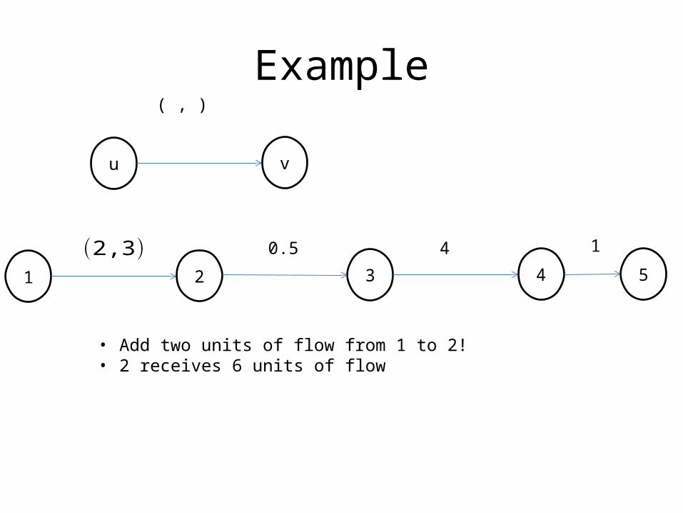
Example

u v

( , )

1 2 3 4 5(2,3) 0.5 4 1

• Add two units of flow from 1 to 2!• 2 receives 6 units of flow

Example

u v

( , )

1 2 3 4 53 (6,0.5) 4 1

• 2 send its 6 unit of flow out!• 3 receives 3 units of flow

Example

u v

( , )

1 2 3 4 53 0.5 (3,4) 1

• 3 send its 3 unit of flow out!• 4 receives 12 units of flow

Example

u v

( , )

1 2 3 4 53 0.5 4 (12,1)

• 4 send its 12 unit of flow out!• 5 receives 12 units of flow • 2 units were first sent, and eventually 12 were

received. Notice the relation is 6

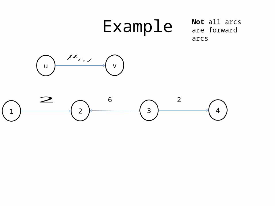
Example

u v𝜇𝑖 , 𝑗

1 2 3 42 6 2

Not all arcs are forward arcs

Example

1 2 3 4(1,2) 6 2

• Add one units of flow from 1 to 2!• 2 receives 2 units of flow

u v

( , )

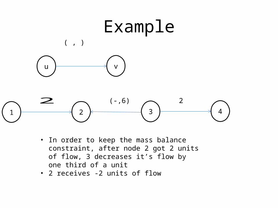
Example

1 2 3 42 (-,6) 2

• In order to keep the mass balance constraint, after node 2 got 2 units of flow, 3 decreases it’s flow by one third of a unit

• 2 receives -2 units of flow

u v

( , )

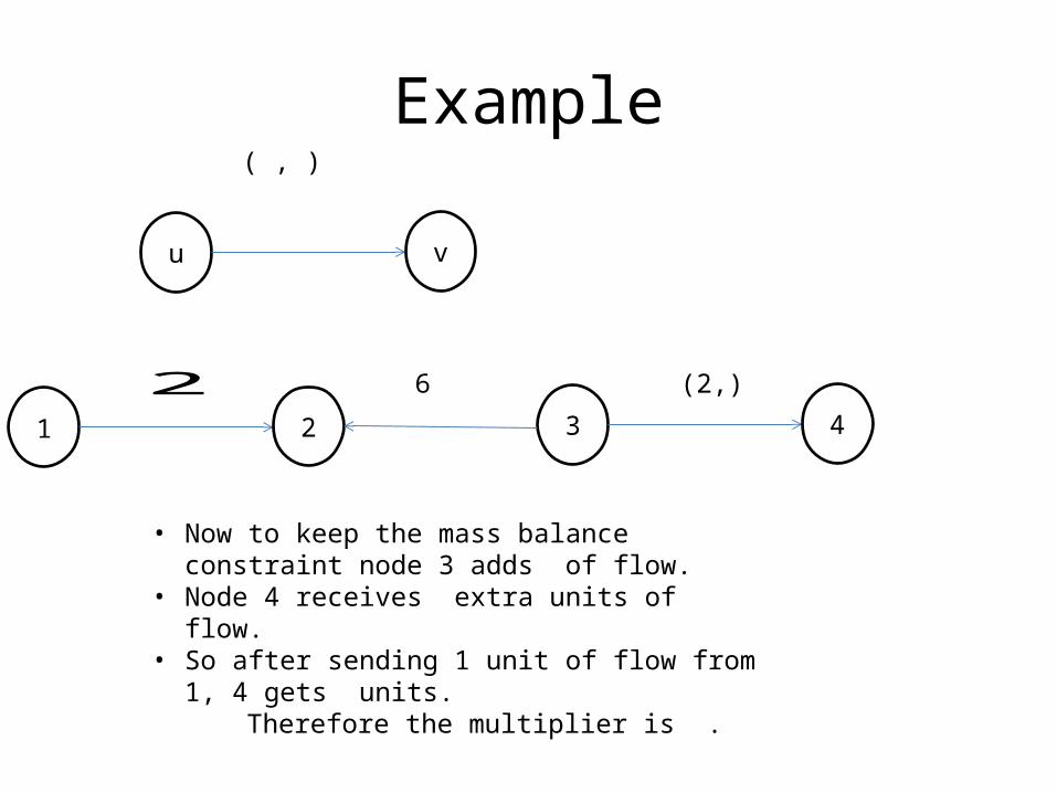
Example

1 2 3 42 6 (2,)

• Now to keep the mass balance constraint node 3 adds of flow.

• Node 4 receives extra units of flow.• So after sending 1 unit of flow from 1, 4 gets units. Therefore the multiplier is .

u v

( , )

Conclusion

• Property 1: If we send 1 unit of flow from node s to another node t along a path P, then units become available at node t.

Flows along Cycles

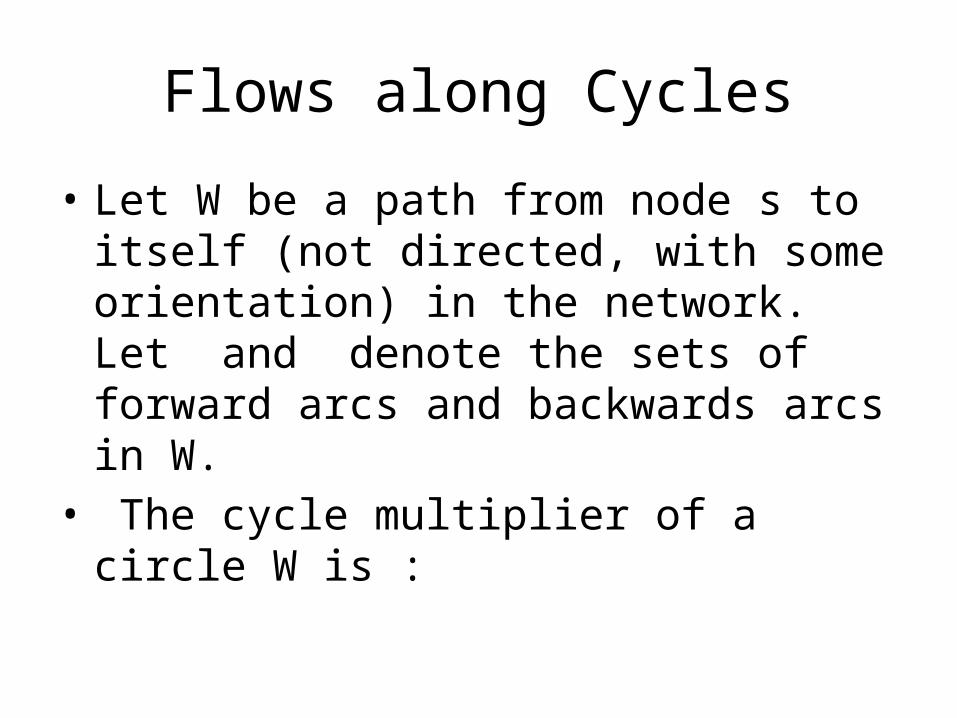
• Let W be a path from node s to itself (not directed, with some orientation) in the network. Let and denote the sets of forward arcs and backwards arcs in W.

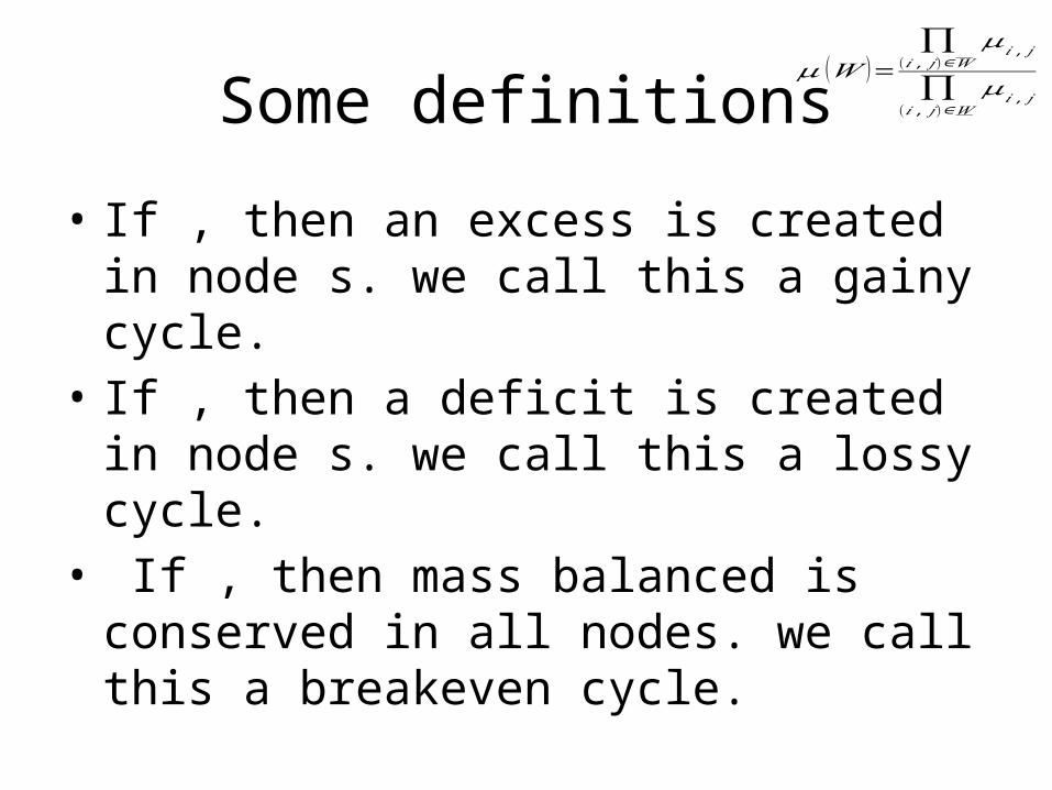
• The cycle multiplier of a circle W is :

Some definitions

• If , then an excess is created in node s. we call this a gainy cycle.

• If , then a deficit is created in node s. we call this a lossy cycle.

• If , then mass balanced is conserved in all nodes. we call this a breakeven cycle.

𝜇 (𝑊 )=∏

(𝑖 , 𝑗 )∈𝑊𝜇𝑖 , 𝑗

∏(𝑖 , 𝑗 )∈𝑊

𝜇𝑖 , 𝑗

• Property 2: if is the multiplier of a cycle W with a particular orientation, then is the multiplier of the same cycle with opposite direction

Proof: nominator and denominator switch by definition. • Property 3: if the cycle is loosy with one

orientation and gainy with the other.

𝜇 (𝑊 )=∏

(𝑖 , 𝑗 )∈𝑊𝜇𝑖 , 𝑗

∏(𝑖 , 𝑗 )∈𝑊

𝜇𝑖 , 𝑗

• Property 4: By sending units along a nonbreakeven cycle starting at node s, we create an imbalance of units at node s.

Proof: at first we send units, and then by property 1, units arrive back at node s, so the size of the imbalance is -

Reminder:Property 1: If we send 1 unit of flow from node s to another node t along a path P, then units become available at node t.

Augmented Tree

• Let be a subgraph of such that and . • is considered an augmented tree if is a

spanning tree of together with some extra edge which is called the extra arc

• An augmented tree has a designated node called the root. Each augmented tree is hanging from it’s root

Example

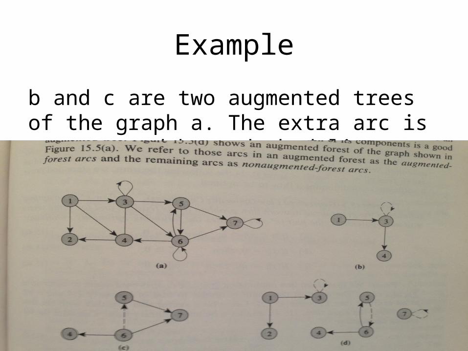
b and c are two augmented trees of the graph a. The extra arc is represented by a dashed line

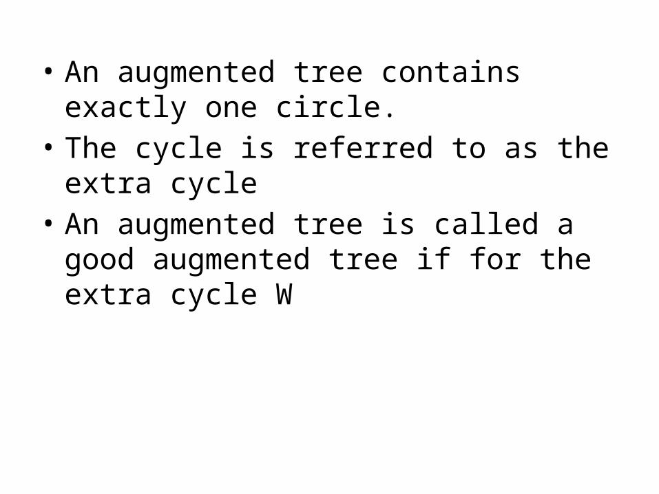
• An augmented tree contains exactly one circle.• The cycle is referred to as the extra cycle• An augmented tree is called a good

augmented tree if for the extra cycle W

Augmented Forest

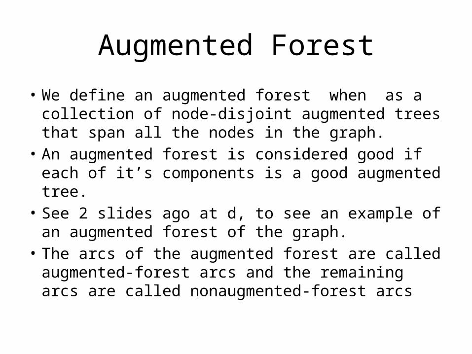
• We define an augmented forest when as a collection of node-disjoint augmented trees that span all the nodes in the graph.

• An augmented forest is considered good if each of it’s components is a good augmented tree.

• See 2 slides ago at d, to see an example of an augmented forest of the graph.

• The arcs of the augmented forest are called augmented-forest arcs and the remaining arcs are called nonaugmented-forest arcs

Augmented Forest Structures and Optimality Conditions

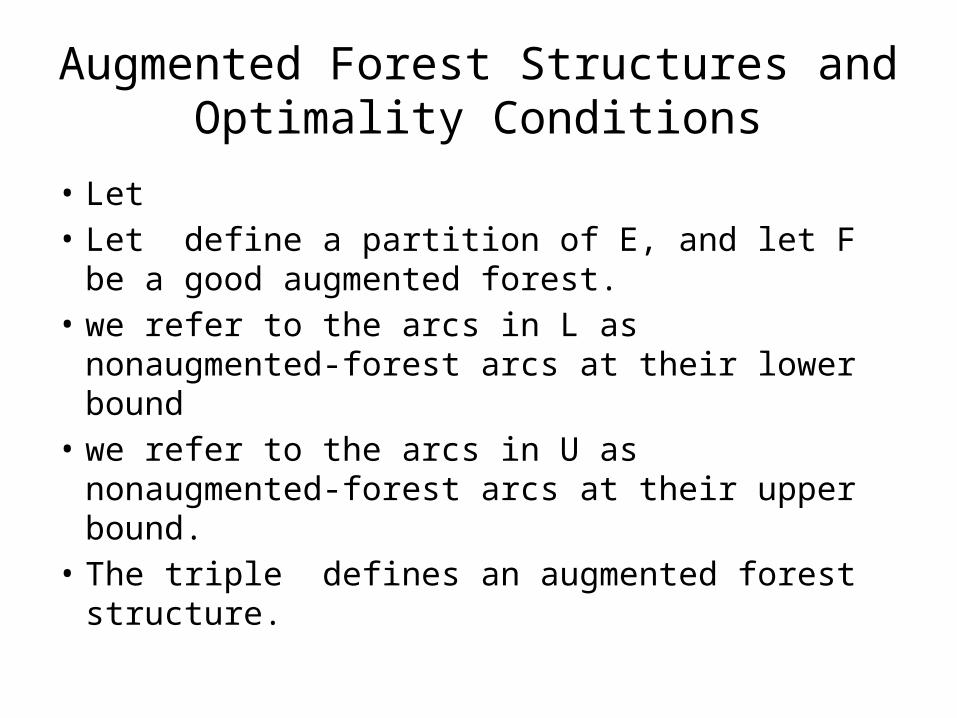
• Let • Let define a partition of E, and let F be a good

augmented forest.• we refer to the arcs in L as nonaugmented-

forest arcs at their lower bound• we refer to the arcs in U as nonaugmented-

forest arcs at their upper bound.• The triple defines an augmented forest

structure.

Feasibility

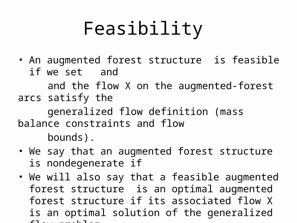
• An augmented forest structure is feasible if we set and and the flow X on the augmented-forest arcs satisfy the generalized flow definition (mass balance constraints and flow bounds).• We say that an augmented forest structure is nondegenerate

if • We will also say that a feasible augmented forest structure is

an optimal augmented forest structure if its associated flow X is an optimal solution of the generalized flow problem

Node Potentials and Reduced Costs

• Let be the node potentials function• With respect to , we define the reduced cost

of an arc as :

Generalized Flow Optimality Condition

• A flow x* is an optimal solution of the generalized network flow problem if it is feasible and for some potential function the following conditions are satisfied:

1. If then 2. If then 3. If then

Proof

Claim 1 : minimizing is equivalent to minimizing Similar to a proof was given in the past

Back to the sentence: let x be some arbitrary flow.

Looking at Let’s prove that each term in the summation is not negative:Lets look at the following 3 cases to prove this:1. in this case it is given that 2. in this case =0, and because , we multiply two

non negative numbers so the result is not negative.

3. in this case =, and because , we multiply two non positive numbers so the result is not negative.

1. If then 2. If then 3. If then

So now , which means that .We showed that with the 3 conditions, some feasible flow is minimal.

Augmented Forest Structure Optimality Conditions

This property’s proof is immediate from the last sentence: • A feasible augmented forest structure with the

associated flow is an optimal augmented forest structure if for some function the pair satisfy the following optimality conditions:

1. (because ) 2. (because ) 3. (because )

Determining Node Potentials for an Augmented Forest Structure

• Let be an augmented forest structure. The augmented forest F contains several augmented trees.

• The following algorithm is performed per tree.• Let be some augmented tree, and let node h

be it’s root. • We would like to satisfy the condition that , so

we use the following equation:

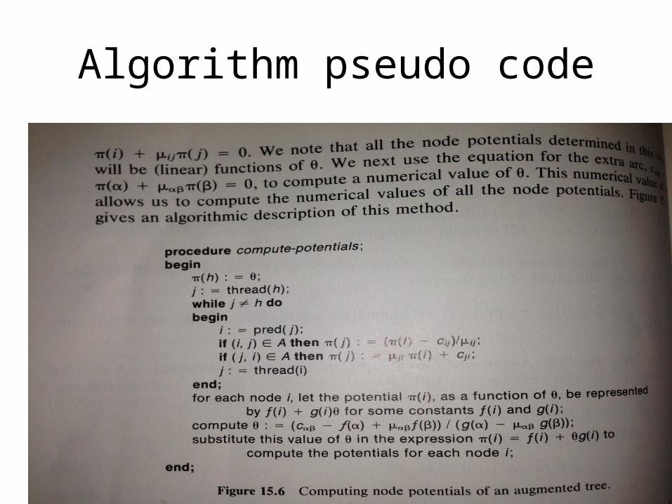
The main idea

• We start by setting which will be determined later.

• We then use DFS on the not directed tree T, and because of connectivity and DFS properties, we will always know or when , so for each node we will get a single equation with one variable (and ).

• We use the extra arc to determine , and update the potentials (they are linear functions of ).

Algorithm pseudo code

Example

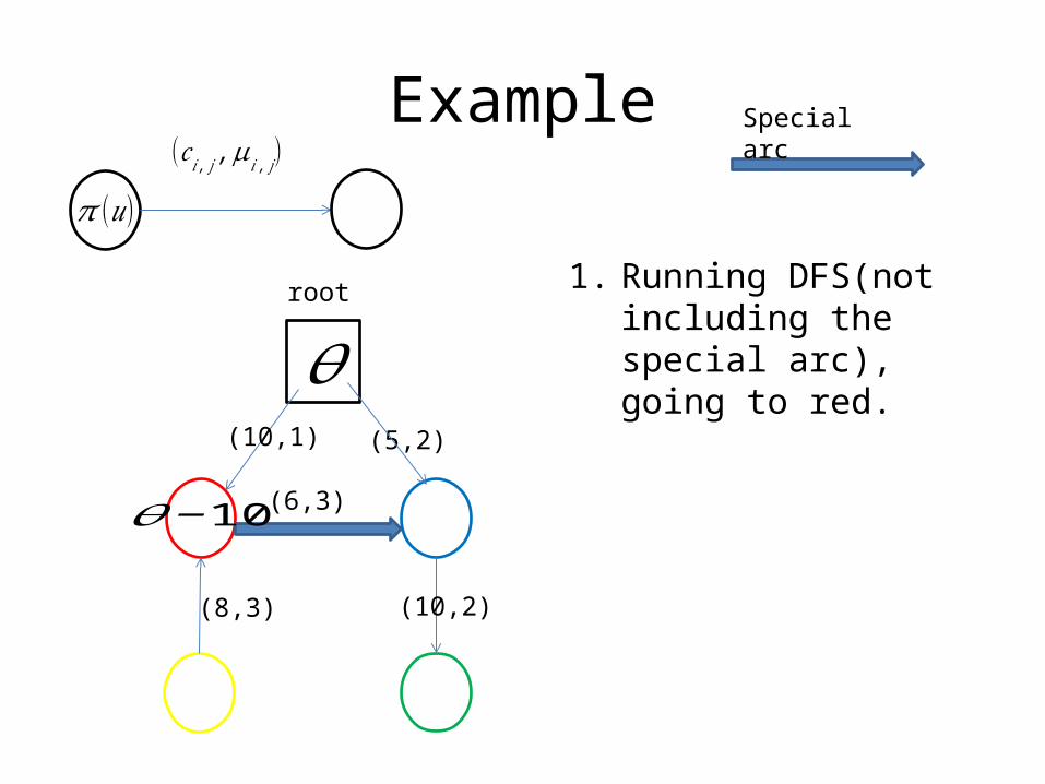
u v

(𝑐 𝑖 , 𝑗 ,𝜇𝑖 , 𝑗)Special arc

(10,1) (5,2)

(8,3)

(6,3)

(10,2)

Example(𝑐 𝑖 , 𝑗 ,𝜇𝑖 , 𝑗)

𝜃

Special arc

(10,1)

(10,2)

(5,2)

(8,3)

(6,3)

Determine root

𝜋 (𝑢)

Example(𝑐 𝑖 , 𝑗 ,𝜇𝑖 , 𝑗)

𝜃

Special arc

(10,1)

(10,2)

(5,2)

(8,3)

(6,3)

1. Running DFS(not including the special arc), going to red.

root

𝜋 (𝑢)

𝜃−10

Example(𝑐 𝑖 , 𝑗 ,𝜇𝑖 , 𝑗)

𝜃

Special arc

(10,1)

(10,2)

(5,2)

(8,3)

(6,3)

1. Running DFS(not including the special arc), going to yellow.

root

𝜋 (𝑢)

𝜃−10

3 𝜃−22

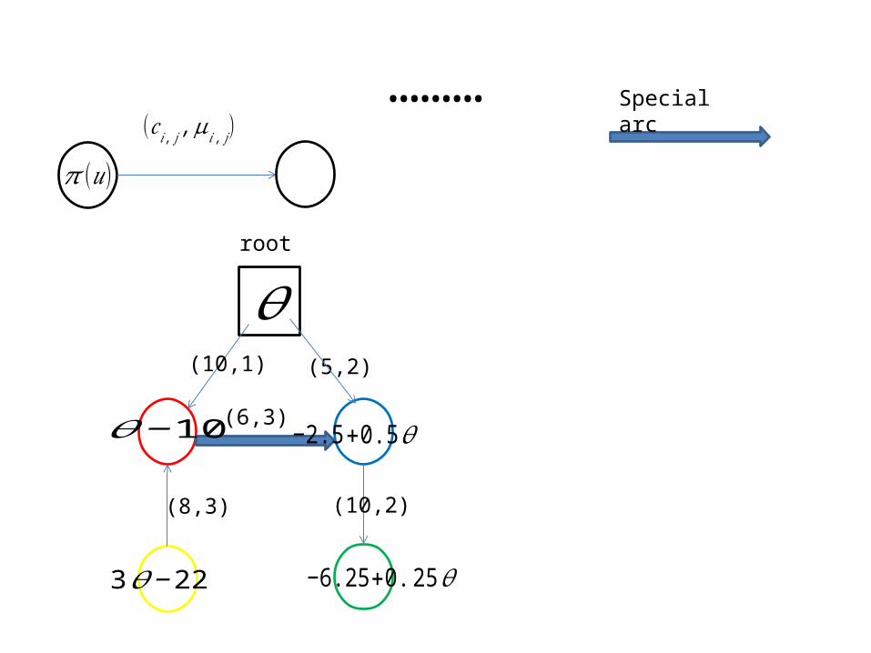
………(𝑐 𝑖 , 𝑗 ,𝜇𝑖 , 𝑗)

𝜃

Special arc

(10,1)

(10,2)

(5,2)

(8,3)

(6,3)

root

𝜋 (𝑢)

𝜃−10

3 𝜃−22

−2.5+0.5 𝜃

−6.25+0.25 𝜃

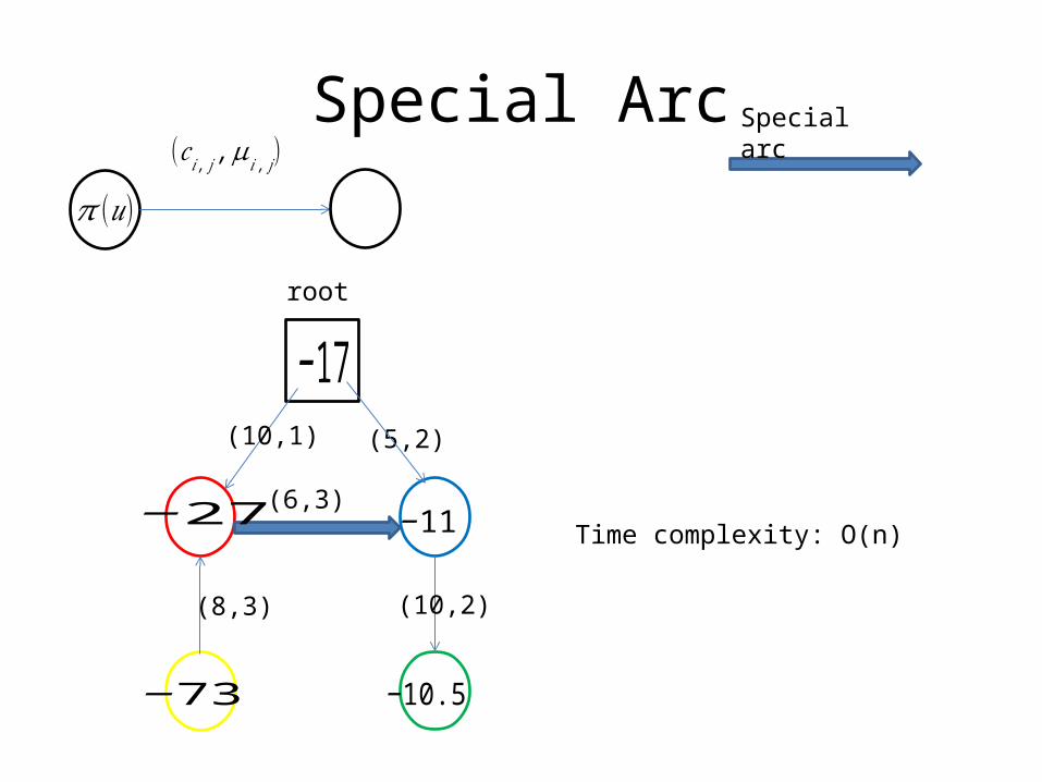
Special Arc(𝑐 𝑖 , 𝑗 ,𝜇𝑖 , 𝑗)

−17

Special arc

(10,1)

(10,2)

(5,2)

(8,3)

(6,3)

root

𝜋 (𝑢)

−27

−73

−11

−10.5

Time complexity: O(n)

Determining Flow for an Augmented Forest Structure

• Let be an augmented tree structure with the current assumption that the network is uncapacitated, which means .

• We present an algorithm determining the flow for each augmented tree.

• In this algorithm we start from the leaf nodes, and advance toward the root.

• Let be some augmented tree of the forest.• We define as the imbalance of a node, and

begin with .• We set the flow of the extra arc and all other

arcs get flow 0.• We can say we decreased the imbalance at

node a by units, and increased it at node b by units.

• Now we start updating the graph in the following way:

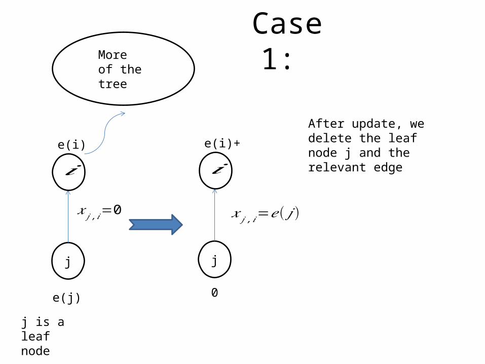
Case 1:

j

e(j)

𝑖

e(i)

More of the tree

j is a leaf node

j

𝑖

e(i)+

0

𝑥 𝑗 ,𝑖=0 𝑥 𝑗 ,𝑖=𝑒( 𝑗)

After update, we delete the leaf node j and the relevant edge

Case 2:

j

e(j)

𝑖

e(i)

More of the tree

j is a leaf node

j

𝑖

e(i)+

0

𝑥𝑖 , 𝑗=0 𝑥𝑖 , 𝑗=−𝑒( 𝑗)𝜇𝑖 , 𝑗

After update, we delete the leaf node j and the relevant edge

• After updating the rest of the leaves (each time we get a new tree ) each arc is a function of

• we set , calculate the value of , and place it in all of the arcs flows.

• Now we have a flow that satisfy the mass balance constraint (if all arcs were not capacitated)

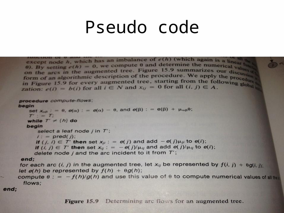
Pseudo code

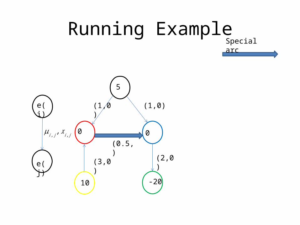
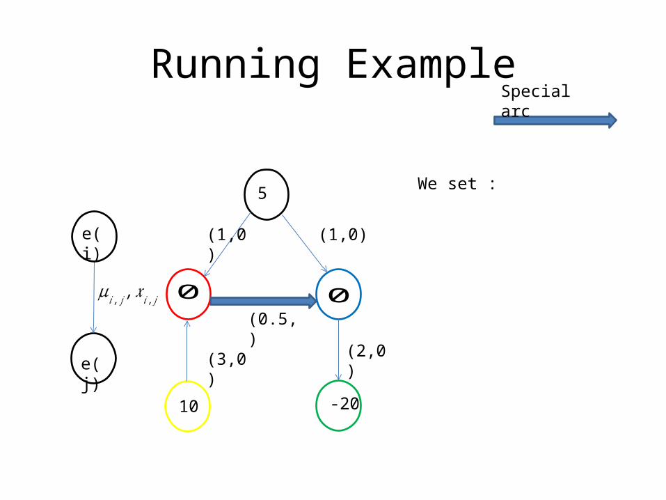
Running Example

𝜇𝑖 , 𝑗 ,𝑥 𝑖 , 𝑗

e(i)

e(j)

Special arc

(1,0)

0 0

10 -20

(3,0) (2,0)

5

(1,0)

(0.5, )

Running Example

𝜇𝑖 , 𝑗 ,𝑥 𝑖 , 𝑗

e(i)

e(j)

Special arc

(1,0)

0 0

-20

(3,0) (2,0)

5

(1,0)

(0.5, )

We set :

10

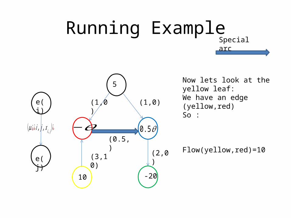
Running Example

(𝜇¿¿ 𝑖 , 𝑗 ,𝑥 𝑖 , 𝑗)¿

e(i)

e(j)

Special arc

(1,0)

−𝜃 0.5 𝜃

-20

(3,10) (2,0)

5

(1,0)

Now lets look at the yellow leaf:We have an edge (yellow,red)So :

Flow(yellow,red)=10(0.5, )

10

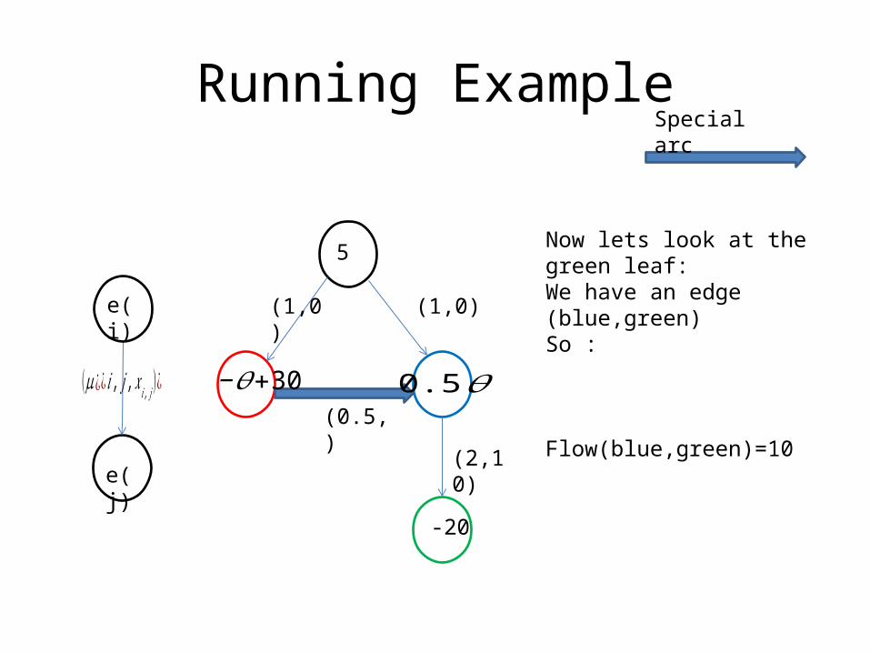
Running Example

(𝜇¿¿ 𝑖 , 𝑗 ,𝑥 𝑖 , 𝑗)¿

e(i)

e(j)

Special arc

(1,0)

−𝜃+30 0.5 𝜃

-20

(2,10)

5

(1,0)

Now lets look at the green leaf:We have an edge (blue,green)So :

Flow(blue,green)=10(0.5, )

Running Example

(𝜇¿¿ 𝑖 , 𝑗 ,𝑥 𝑖 , 𝑗)¿

e(i)

e(j)

Special arc

(1,0)

−𝜃+30 0.5 𝜃−10

5

(1,0)

Now lets look at the blue leaf:We have an edge (black,blue)So :

Flow(black,blue)=(0.5, )

Running Example

(𝜇¿¿ 𝑖 , 𝑗 ,𝑥 𝑖 , 𝑗)¿

e(i)

e(j)

Special arc

−𝜃+30

0.5 𝜃−5

(1,0)

Now lets look at the red leaf:We have an edge (black,red)So :

Flow(black,red)=

Now to determine :

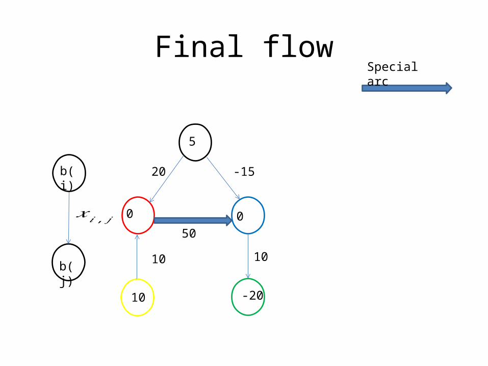
Final flow

𝑥𝑖 , 𝑗

b(i)

b(j)

Special arc

-15

0 0

-20

10 10

5

20

50

10

• It is easy to prove this algorithm finds a unique flow and value of .

• Eventually we get some linear function of for • It is important to show that g(root) is never 0.

Proof:

• It is easy to see that is the imbalance of the root, resulting from setting the flow on the arc as

• Setting the flow on the arc as creates a deficit of units at a, and an excess of at b. let denote the tree path from x to y, and let denote the path multiplier.

• We can cancel the deficit at node a by sending from the root, and cancel the excess at node b by sending from node b to the root ( units arrive at the root)

• So using the last conclusions we can say that g(root)=

• So g(root)==1, but this is exactly the multiplier of the circle.

So if the circle is not breakeven (i.e the augmented tree is good), the proof stands.

Extending to capacitated case

1. The initialization is the same.2. For every do begin :setting the required flow : set deficit : set excess.

3. Run the previous algorithm

Conclusion about the flow

• We need the augmented trees to be good augmented tree.

• Our flow satisfy mass balance constraint, but doesn’t promise the flow is legitimate (e.g. negative flow as seen in example)

• The flow on the arcs of the augmented forest that satisfy the mass balance constraint is unique, so the forest structure is feasible if and only if the flow bounds are satisfied

Properties from linear programming (no proof)

• Arcs in a set B have a unique solution if and only if B is a good augmented forest

• A set B of arcs defines a basis(an extreme point on the polytope) of the generalized network problem if and only if B is a good augmented forest.

This means that there exist an optimal solution for a good augmented tree.

The Generalized Network Simplex Algorithm

• This algorithm maintains a good feasible augmented forest structure at every iteration, using pivot rules to eventually reach an improved augmented forest structure that satisfies the optimality conditions

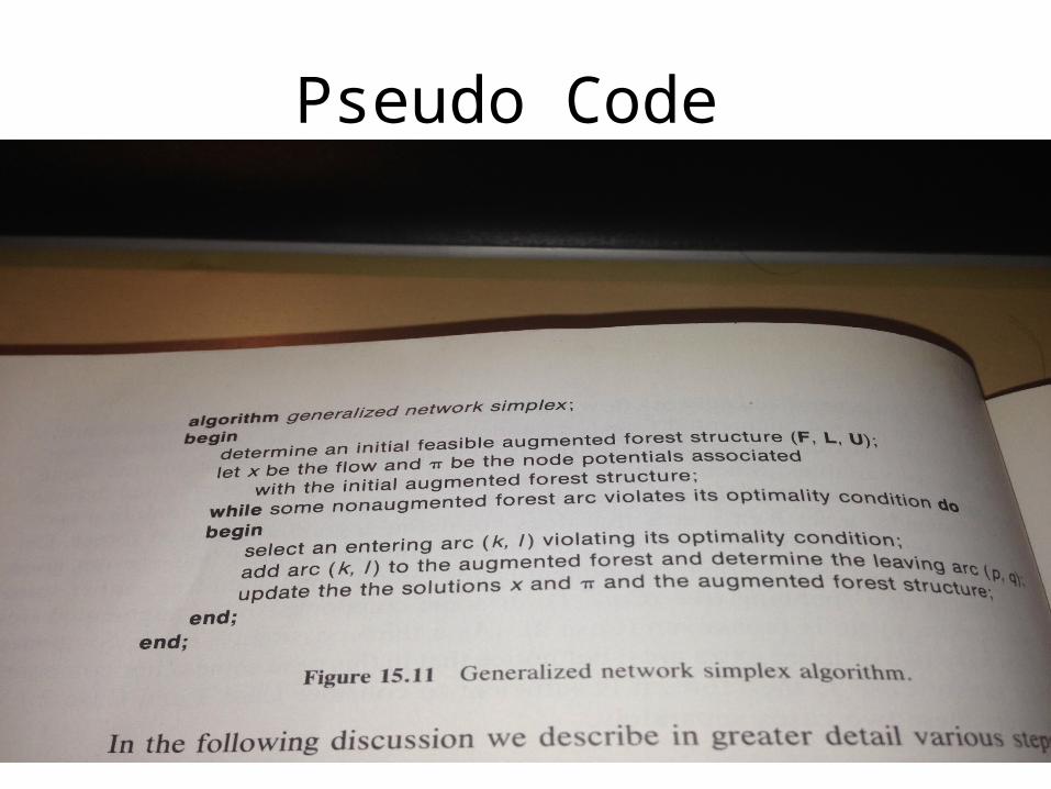
Pseudo Code

Obtaining an Initial Good Augmented Forest Structure

• Easy to achieve an artificial initial augmented forest structure, simply by adding self edges with sufficiently large cost, infinite capacity and appropriate multipliers on these edges.

• We will avoid full details and proof but assume we have a good initial augmented forest structure.

• Computing x and like explained in previous slides.

Initial Augmented Forest

0 0

-20

5

10

(𝜇¿¿ 𝑖 , 𝑖 ,𝑐 𝑖 , 𝑖 ,𝑢𝑖 , 𝑗)¿

b(i)

(0.5

(2 (2

(2(0.5

The forest is the set of self arcs.

Set

M is big enough so that if a feasible solution exists, no optimal solution with positive flow on the self arcs exists.

Optimality Testing and the Entering Arc

To determine whether a spanning tree structure is optimal we check:

If the spanning tree structure satisfies the conditions it is optimal

we terminate

Else, the algorithm selects a non-forest violating arc to enter the forest:

70

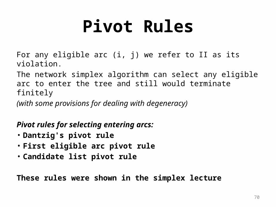
Pivot Rules

For any eligible arc (i, j) we refer to II as its violation.The network simplex algorithm can select any eligible arc to enter the tree and still would terminate finitely(with some provisions for dealing with degeneracy)

Pivot rules for selecting entering arcs:• Dantzig's pivot rule• First eligible arc pivot rule• Candidate list pivot rule

These rules were shown in the simplex lecture

Identifying the Leaving Arc

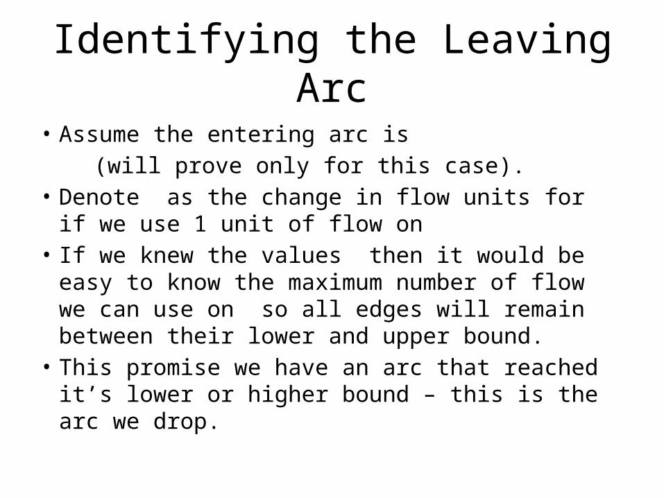
• Assume the entering arc is (will prove only for this case).• Denote as the change in flow units for if we use 1

unit of flow on • If we knew the values then it would be easy to know

the maximum number of flow we can use on so all edges will remain between their lower and upper bound.

• This promise we have an arc that reached it’s lower or higher bound – this is the arc we drop.

Determine

• Use the Algorithm presented before to compute the value of each arc in the trees of k,l:

• At first the flow is 0 for all edges, and the imbalance vector is:

e(i) = -1 if i=k e(i) = if i=l e(i) = 0 else The arc flow we obtain are the values

Determine the Maximum Flow On (k,l) Within the Bounds

• If we add units of flow to (k,l) then to keep the flow bounds :

• It is easy to see that if then the edge will go up to it’s lower bound, and if then the opposite will happen.

• Denote by the maximum number of units allowed to use to make reach it’s lower\upper bound then:

• So the largest value for which is feasible is

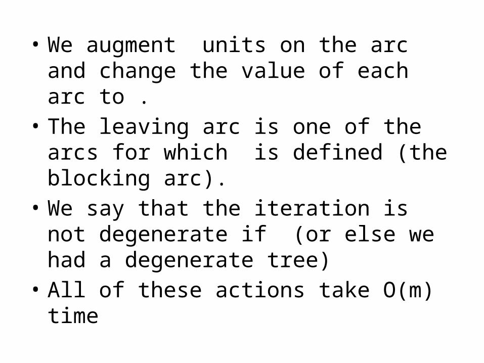
• We augment units on the arc and change the value of each arc to .

• The leaving arc is one of the arcs for which is defined (the blocking arc).

• We say that the iteration is not degenerate if (or else we had a degenerate tree)

• All of these actions take O(m) time

Updating the Augmented Forest

• When leaving arc (p, q) is determined for a given entering arc (k, I), we updates the tree structure

• If the leaving arc is the same as the entering arc, (when δ = δpq =upq), the tree does not change.-the arc (k, I) merely moves from the set L to the set U, or vice versa.

• If the leaving arc differs from the entering arc, we need to prove we still have a good augmented forest. We use the fact that the simplex method moves from one basis to another, and each basis is a good augmented forest.

Updating Potentials, Tree Indices

• Use the node potential algorithm presented before for the new tree(s) O(n) time.

• Update the tree indices – can do it from scratch in O(n) time.

Termination (1)

• The Algorithm moves from one feasible augmented forest structure to the other until it satisfies the optimality conditions.

• In a pivot operation, the objective function value decreases by the amount of at every iteration (no proof)

• If each pivot operation is nondegenrate (i.e ) each subsequent augmented forest structure has a smaller cost.

Termination (2)

• Since any network has a finite number of augmented forest structures, and each augmented forest structure has a unique associated cost(which decreases with every iteration), the generalized network simplex algorithm terminates.

Dealing with Degenerate Pivots

• We define as an n-vector whose elements are for a sufficiently small real number .

• If we replace by it is possible to prove that the augmented forest structure at every iteration is not degenerate and therefore the algorithm terminates.

• It is also possible to prove that an optimal augmented forest structure of the perturbed problem is also an optimal augmented forest structure of the original problem.

Complexity• #of iterations * complexity of iteration.• Cannot bound the number of iterations by any polynomial p(n,m).• In practice the number of iterations is generally a low order

polynomial p(n,m).• All of the operations: identifying the entering arc, computing

values, updating flows, potentials and tree indices require O(m) time.

So in practice the time complexity is a low order polynomial p(n,m).• Empirical investigations found that the generalized network simplex

algorithm is 2 to 3 times slower than that of the minimal cost simplex algorithm.

An Application Example

• Sally owns a warehouse of fixed capacity 1000 units to store a type of wine whose price is unstable

• She knows the price of the product for the next 3 time periods, and she needs to manage her purchases, sales and storage patterns.

• Suppose she holds units of the wine, and she has dollars in assets.

• In each period she can sell and buy wine under the limitations.• The price of the wine varies(we define it as at time i) and

ultimately all of the wine must be sold.• The idea is to maximize the amount of cash available at the end

of the third period.

, )Warehouse:Can store 1000 units of wine=10,000$

1 2 3v

1’ 2’ 3’ 4’

sell sell sell

buy buy

u v

(𝑐𝑜𝑠𝑡 ,𝑐𝑎𝑝𝑎𝑐𝑖𝑡𝑦 ,𝑚𝑢𝑙𝑡𝑖𝑝𝑙𝑖𝑒𝑟 )

(𝑖𝑛𝑣𝑒𝑛𝑡𝑜𝑟𝑦h𝑜𝑙𝑑𝑖𝑛𝑔$

𝑢𝑛𝑖𝑡,1000 ,1)

(0 ,∞ ,𝑏𝑎𝑛𝑘 𝑖𝑛𝑡𝑟𝑒𝑠𝑡)

(0 ,∞ ,𝑝3)(0 ,∞ ,

1𝑝1

)

Flow represent wine quantity here

Flow represent $ here

The End