Cambridge Part III MathsMichaelmas 2015

General Relativity

based on a course given by written up byUlrich Sperhake Josh Kirklin

Please send errors and suggestions to jjvk2@cam.ac.uk.

Contents1 The Equivalence Principles 2

1.1 Statement of the equivalence principle . . . . . . . . . . . . . . . . . . . . . . . . . 31.2 Bending of light . . . . . . . . . . . . . . . . . . . . . . . . . . . . . . . . . . . . . . 41.3 Gravitational redshift . . . . . . . . . . . . . . . . . . . . . . . . . . . . . . . . . . 41.4 Curved spacetimes . . . . . . . . . . . . . . . . . . . . . . . . . . . . . . . . . . . . 5

2 Manifolds and Tensors 52.1 Differentiable manifolds . . . . . . . . . . . . . . . . . . . . . . . . . . . . . . . . . 52.2 Smooth functions . . . . . . . . . . . . . . . . . . . . . . . . . . . . . . . . . . . . . 62.3 Curves and vectors . . . . . . . . . . . . . . . . . . . . . . . . . . . . . . . . . . . . 72.4 Covectors/1-forms . . . . . . . . . . . . . . . . . . . . . . . . . . . . . . . . . . . . 82.5 Abstract index notation . . . . . . . . . . . . . . . . . . . . . . . . . . . . . . . . . 92.6 Tensors . . . . . . . . . . . . . . . . . . . . . . . . . . . . . . . . . . . . . . . . . . 92.7 Tensor fields . . . . . . . . . . . . . . . . . . . . . . . . . . . . . . . . . . . . . . . . 122.8 The commutator . . . . . . . . . . . . . . . . . . . . . . . . . . . . . . . . . . . . . 132.9 Integral curves . . . . . . . . . . . . . . . . . . . . . . . . . . . . . . . . . . . . . . 13

3 The Metric Tensor 143.1 Lorentzian signature . . . . . . . . . . . . . . . . . . . . . . . . . . . . . . . . . . . 163.2 Curves of extremal time . . . . . . . . . . . . . . . . . . . . . . . . . . . . . . . . . 173.3 Covariant derivative . . . . . . . . . . . . . . . . . . . . . . . . . . . . . . . . . . . 183.4 Higher derivatives . . . . . . . . . . . . . . . . . . . . . . . . . . . . . . . . . . . . 203.5 The Levi-Civita connection . . . . . . . . . . . . . . . . . . . . . . . . . . . . . . . 203.6 Geodesics . . . . . . . . . . . . . . . . . . . . . . . . . . . . . . . . . . . . . . . . . 213.7 Normal coordinates . . . . . . . . . . . . . . . . . . . . . . . . . . . . . . . . . . . . 22

4 Physical Laws in Curved Spacetime 234.1 Covariance . . . . . . . . . . . . . . . . . . . . . . . . . . . . . . . . . . . . . . . . 234.2 Energy-momentum tensor . . . . . . . . . . . . . . . . . . . . . . . . . . . . . . . . 24

– 1 –

1 The Equivalence Principles

5 Curvature 255.1 Parallel transport . . . . . . . . . . . . . . . . . . . . . . . . . . . . . . . . . . . . . 255.2 The Riemann tensor . . . . . . . . . . . . . . . . . . . . . . . . . . . . . . . . . . . 265.3 Parallel transport and curvature . . . . . . . . . . . . . . . . . . . . . . . . . . . . 265.4 Symmetries of the Riemann tensor . . . . . . . . . . . . . . . . . . . . . . . . . . . 275.5 Geodesic deviation . . . . . . . . . . . . . . . . . . . . . . . . . . . . . . . . . . . . 275.6 Curvature of the Levi-Civita connection . . . . . . . . . . . . . . . . . . . . . . . . 285.7 Einstein’s equation . . . . . . . . . . . . . . . . . . . . . . . . . . . . . . . . . . . . 29

6 Diffeomorphisms and Lie derivatives 296.1 Maps between manifolds . . . . . . . . . . . . . . . . . . . . . . . . . . . . . . . . . 296.2 Diffeomorphisms and diffeomorphism invariance . . . . . . . . . . . . . . . . . . . . 316.3 Lie derivatives, symmetries . . . . . . . . . . . . . . . . . . . . . . . . . . . . . . . 32

7 Linearised Theory 347.1 The linearised Einstein equations . . . . . . . . . . . . . . . . . . . . . . . . . . . . 347.2 Newtonian limit . . . . . . . . . . . . . . . . . . . . . . . . . . . . . . . . . . . . . . 357.3 Gravitational waves . . . . . . . . . . . . . . . . . . . . . . . . . . . . . . . . . . . 367.4 The field far from the source . . . . . . . . . . . . . . . . . . . . . . . . . . . . . . 377.5 Energy in gravitational waves . . . . . . . . . . . . . . . . . . . . . . . . . . . . . . 387.6 Quadrupole formula . . . . . . . . . . . . . . . . . . . . . . . . . . . . . . . . . . . 40

8 Differential Forms 408.1 p-forms . . . . . . . . . . . . . . . . . . . . . . . . . . . . . . . . . . . . . . . . . . 408.2 Integration . . . . . . . . . . . . . . . . . . . . . . . . . . . . . . . . . . . . . . . . 418.3 Submanifolds, Stokes’ theorem . . . . . . . . . . . . . . . . . . . . . . . . . . . . . 42

9 The Initial Value Problem 439.1 Extrinsic curvature . . . . . . . . . . . . . . . . . . . . . . . . . . . . . . . . . . . . 439.2 The Gauss-Codazzi equations . . . . . . . . . . . . . . . . . . . . . . . . . . . . . . 449.3 The constraint equations . . . . . . . . . . . . . . . . . . . . . . . . . . . . . . . . . 459.4 Foliations . . . . . . . . . . . . . . . . . . . . . . . . . . . . . . . . . . . . . . . . . 459.5 The 3 + 1 equations . . . . . . . . . . . . . . . . . . . . . . . . . . . . . . . . . . . 46

10 The Lagrangian Formulation 47

1 The Equivalence PrinciplesGeneral relativity arises from an incompatibility between special relativity and Newtonian gravity.In special relativity, physical laws must be the same in any “inertial frame”, i.e. to any of aset of non-accelerating observers related by Lorentz transformations. Newtonian gravity can besummarised by Poisson’s equation

∇2φ = 4πGρ =⇒ φ(t,x) = −G∫

ρ(t,y)|x− y| d

3y .

Lorentz transformations mix space and time coordinates, so Poisson’s equation in general is notinvariant under Lorentz transformations. Additionally, special relativity imposes a finite propagationspeed for any signals, but Newtonian gravity allows instantaneous information transmission.

– 2 –

1 The Equivalence Principles 1.1 Statement of the equivalence principle

Experimentally we know that Newtonian gravity is a good approximation if v c. Consider forexample a test particle in a circular orbit of a planet of mass M . The gravitational potential isφ = −GM

r , and balancing gravity with radial acceleration we obtain v2

r = GMr . Hence v c ⇐⇒

Gc2Mr 1, and this is true for the solar system in which we typically have G

c2Mr < 10−5.

1.1 Statement of the equivalence principleIn Newtonian theory, we have two types of mass. There is the inertial mass, present in Newton’ssecond law F = mI x, and the gravitational mass, present in the equation for the gravitational forceF = mGg, where g = −∇φ. We observe that (with suitable scaling) mI differs from mG by atmost one part in 1012 (e.g. the Eotvos experiment) for all kinds of objects. The weak equivalenceprinciple (WEP) is then to take that they are identical mI = mG = m.For Newtonian motion, the WEP implies x = g, so a second way to state it is: “the trajectory of afreely falling test particle depends only on its original position and velocity and is independent ofits composition”.Let O be an inertial frame with coordinates (t,x) in a gravitational field g, and let O′ be a framewith relative acceleration a to O, with coordinates (t,x′ = x− x0(t)). x0(t) is the position of theorigin of O′ in the coordinates of O, x0 = a. The equation of motion in O′ is x′ = g − a. Notethat we effectively now have a different gravitational field g′ = g − a. Uniform acceleration isindistinguisable from a gravitational field. If a = g, then g′ = 0 and we say that O′ is a freelyfalling frame.A local inertial frame is a coordinate frame (t,x) defined by a freely falling observer in the sameway as Minkowski spacetime, just in a “small” region. Here “local” and “small” are compared withlength scales on which g varies. For instance consider the presence of tidal forces in a lab abovethe Earth:

Earth frame

lab frame

In the frame of the lab, g varies significantly over the lab, so the lab frame is too “large” to beconsidered a local inertial frame.The WEP was found in Newtonian physics. Einstein promoted it to be more general. The Einsteinequivalence principle is in two parts:

1. The WEP is valid.

2. In a local inertial frame, the results of all non-gravitational experiments are indistinguisablefrom those of the same experiment in an inertial frame in Minkowski spacetime.

(“Schiff’s conjecture” is that the WEP implies the EEP, but this has not actually been proven.)Henceforth we will assume the EEP.

– 3 –

1 The Equivalence Principles 1.2 Bending of light

1.2 Bending of lightConsider a freely falling laboratory in a uniform gravitational field. Inside the lab, light moves in astraight line, since the lab frame is a locally inertial one. Transforming to the Earth frame, wesee that the light must take a curved path. It travels a horizontal distance given by d = ct, anda vertical distance given by gt2/2. Hence the height of the light is given by h = gd2

2c2 – the lightfollows a parabola.

1.3 Gravitational redshiftConsider a uniform gravitational field g = (0, 0,−g) with two observers, Alice at z = h and Bob atz = 0. Alice sends light signals to Bob. The EEP implies that this is equivalent to a frame withacceleration (0, 0, g). We assume that vA, vB c, so that we can ignore v2

c2 and higher order termsthat arise from special relativity. In the accelerating frame we have

zA(t) = h+ 12gt

2, zB(t) = 12gt

2,

and vA = vB = gt c. Suppose Alice emits the first signal at t = t1. The path of the signal isgiven by

z1(t) = zA(t1)− c(t− t1) = h+ 12gt

21 − c(t− t1).

The signal reaches Bob at t = T1, defined by

h+ 12gt

21 − c(T1 − t1) = 1

2gT21 .

Now suppose Alice emits a second signal at t2 = t1 + ∆τA recieved by Bob at T2 = T1 + ∆τB . Thenwe similarly have

h+ 12g(t1 + ∆τA)2 − c(T1 + ∆τB − t1 −∆τA) = 1

2g(T1 + ∆τB)2.

Subtracting these equations we obtain

c(∆τA −∆τB) + 12g∆τA(2t1 + ∆τA) = 1

2g∆τB(2T1 + ∆τB).

Now we assume that ∆τA t1 and ∆τB T1, as is the case for example when the signals are theconsecutive peaks of light waves. Then we have

c(∆τA −∆τB) + g∆τAt1 = g∆τBT1,

from which we can deduce

∆τB =(

1 + gT1c

)−1 (1 + gt1

c

)∆τA ≈

(1− g(T1 − t1)

c

)∆τA.

Note that we haveh

c− (T1 − t1) = 1

2g

c(T1 + t1)︸ ︷︷ ︸1

(T1 − t1)︸ ︷︷ ︸≈hc

≈ 0,

so to leading order T1 − t1 = hc . Therefore we have

∆τB ≈(

1− gh

c2

)∆τA.

– 4 –

2 Manifolds and Tensors 1.4 Curved spacetimes

The signal appears blueshifted to Bob:

c∆τB = λB ≈(

1− gh

c2

)λA

This was confirmed in the Pound-Rebka experiment (1960). Similarly, light climbing out of agravity well is redshifted. In general, we have

∆τB ≈(

1 + φB − φAc2

)∆τA.

This equation holds for weak non-uniform fields.

1.4 Curved spacetimesThe WEP says that test bodies move in the same way in a gravitational field, regardless of theircomposition i.e. their gravitational “charge” m. This is unlike any other force. Because of this,Einstein made the deduction that gravity must be a feature of spacetime, in particular its geometry.Consider redshift but now in a non-Minkoskian metric

c2 dτ2 =[1 + 2φ(x, y, z)

c2

]c2 dt2 −

[1− 2φ(x, y, z)

c2

](dx2 + dy2 + dz2),

where φc2 1. Alice and Bob are at fixed positions xA and xB, and Alice emits signals at tA and

tA + ∆t. Bob recieves the first signal at tB. When does he see the second one? Note that thespacetime is static (φ is independent of t), so the 2 signals travel on identical trajectories, justshifted in time. Therefore Bob receives the second signal at tB + ∆t But what proper times doAlice and Bob measure? We have

∆τ2A =

(1 + 2φA

c2

)∆t2 and ∆τ2

B =(

1 + 2φAc2

)∆t2,

so we can write∆τA ≈

(1 + φA

c2

)∆t and ∆τB ≈

(1 + 2φA

c2

)∆t,

and we recover the above result:

∆τB ≈(

1 + φBc2

)(1 + φB

c2

)−1∆τA ≈

(1 + φB − φA

c2

)∆τA

2 Manifolds and TensorsIn GR we define spacetime as a manifold. This is trickier that just Minkowski spacetime for severalreasons. In Minkowski spacetime, the presence of inertial frames leads to a preferred set of globalcoordinates, so we can add position vectors, and spacetime has the structure of a vector space. Ina curved spacetime, inertial coordinates are local, and so we have no set of preferred coordinates,and it is not at first obvious how to interpret vectors.

2.1 Differentiable manifoldsWe know how to do calculus in Rn. The goal now is to develop an analog for curved spaces.

– 5 –

2 Manifolds and Tensors 2.2 Smooth functions

Definition. An n-dimensional differentiable manifold is a set M with subsets Oα such that:

1.⋃αOα =M.

2. For all α there is a bijection φα : Oα → Uα ⊂ Rn, where Uα is open.

3. If Oα ∩ Oβ 6= ∅, then φB φ−1α : φα(Oα ∩ Oβ)→ φβ(Oα ∩ Oβ) is a smooth map.

The φα are sometimes called charts, and the set of all charts for a manifold is sometimes called itsatlas. For p ∈ Oα, we often write

φα(p) = (x1α(p), x2

α(p), x3α(p), . . . ) = xµα(p).

These are the coordinates of p; the α is often dropped.A Ck manifold is defined likewise. From now on we’ll assume that all our manifolds are C∞.

Example. • Rn is a manifold with an atlas of one chart φ : (x1, . . . , xn) 7→ (x1, . . . , xn).

• S1 = (cos θ, sin θ) ∈ R2 s. t. θ ∈ R, the unit circle, is a manifold. There does notexist an atlas for S1 with only one chart. We need two charts. Let P = (1, 0) andQ = (−1, 0). Then two possible such charts are φ1 : S1 \ P → (0, 2π), p 7→ θ andφ2 : S1 \ Q → (−π, π), p 7→ θ.

Definition. Two atlases are compatible iff their union is also an atlas. A complete atlas is theunion of all atlases compatible with a given atlas.

2.2 Smooth functions

Definition. A function f : M → R is smooth provided that for all charts φ the functionF = f φ−1 : U ⊂ Rn → R is smooth.

Sometimes we call f a scalar field.

Example. • For S1 above, f : S1 → R, (x, y) 7→ x is a smooth function.

• Consider a manifold M with a chart φ : O ⊂M→ U ⊂ Rn, p ∈ O 7→ (x1(p), . . . , xn(p)).Let f : O → R, p 7→ x1(p). Then f is smooth.

• We can define f through F . Given an atlas φα then a set of Fα : Uα → R definesf = Fα φα, provided Fα is independent of α on overlapping regions. Note that since wecan go easily between f and F we sometimes abuse notation and do not distinguish them.

– 6 –

2 Manifolds and Tensors 2.3 Curves and vectors

2.3 Curves and vectorsConsider a surface in R3, and the tangent plane at a point p in that surface. The plane has thestructure of a 2D vector space, and a tangent vector to a curve in the surface at p is in the plane.The goal in this section is to formalise this for an n-manifold.

Definition. A smooth curve in a manifold M is a function λ : I →M where I ⊂ R is open,such that φα λ : I → Rn is smooth for all charts φα.

Definition. Let C∞(M,R) be the space of all smooth functions from M→ R, and let λ be asmooth curve with λ(0) = p ∈M. The tangent vector to λ at p is the linear map

Xp : C∞(M,R) → Rf 7→ Xp(f) = d

dtf(λ(t))∣∣∣t=0

.

Tangent vectors are linear and obey the Leibniz rule:

Xp(f + g) = Xp(f) +Xp(g), Xp(αf) = αXp(f), Xp(fg) = Xp(f)g(0) +Xp(g)f(0)

Suppose φ = (xµ) is a chart defined in a neighbourhood of p ∈M and let F = f φ−1. Then wehave

f λ = (f φ−1) (φ λ) = F φ λ,

Xp(f) = ddt(F φ λ)(t)

∣∣∣∣ t = 0

=( dF

dxµ)φ(p)

(dxµ(λ(t))dt

)t=0

= dxµ

dt∂

∂xµF

= ddtF (xµ(λ(t))) = d

dt(f(λ(t))).

For this reason, we call dxµdt the components of the vector, expanded in the basis ∂

∂xµ . We also justrefer to d

dt itself as the vector.

Lemma 1. The set of vectors at p ∈M form an n-dimensional vector space (known as the tangentspace Tp(M)).

The proof is simple.Note that

(∂∂xµ

)p

is not the same as the partial derivative ∂∂µ . Also, the basis

(∂∂xµ

)p

is chartdependent, so we call it the coordinate basis.

Definition. Let eµ be a basis of Tp(M). Then we can expand any vector in this basis,Xp = Xµ

p eµ. Xµp are the components of Xp.

– 7 –

2 Manifolds and Tensors 2.4 Covectors/1-forms

Example. For a coordinate basis, we have Xµp =

(dxµ(λ(t))

dt

)t=0

.

Note that when Einstein convention is applied, we always have one index up and one down (andwe take e.g. ∂

∂xµ to be a “down index”).Let φ = (xµ) and φ = (xµ) be two charts in a neighbourhood of p ∈M. Then we have(

∂

∂xµ

)p

(f) = ∂

∂xµ

(f φ−1

)∣∣∣∣φ(p)

= ∂

∂xµ

[(f φ−1) (φ φ−1)︸ ︷︷ ︸

=xµ(xα)

]∣∣∣∣∣φ(p)

= ∂

∂xµ

[(f φ−1)(x(x))

]∣∣∣∣p

=[∂

∂xα

(f φ−1

)]φ(p)

∂xα

∂xµ

∣∣∣∣φ(p)

=(

∂

∂xα

)p

(f) ∂xα

∂xµ

∣∣∣∣φ(p)

=⇒(

∂

∂xµ

)p

=(∂xα

∂xµ

)φ(p)

(∂

∂xα

)p.

Using this, we can see how the components of a vector transforms when changing between charts.Consider a vector V ∈ Tp(M). We have

V = V µ(

∂

∂xµ

)p

= V µ(∂xα

∂xµ

)φ(p)

(∂

∂xα

)p

= V α(

∂

∂xα

)p,

where V α =(∂xα

∂xµ

)φ(p)

V µ. Vector components transform contravariantly.

2.4 Covectors/1-forms

Definition. Let V be an n-dimensional vector space over R. Its dual space V∗ is the n-dimensional vector space of linear maps V → R. If eµ is a basis of V, then the dual basis, abasis of V∗ is fα, defined by fα(eµ) = δαµ .

V and V∗ are isomorphic. For example eµ 7→ fµ defines an isomorphism. However it is importantto note that this isomorphism must be basis dependent. On the other hand:

Theorem 1. If V is finite dimensional, then a natural, basis independent isomorphism between Vand (V∗)∗ is given by Φ : V → (V∗)∗, X 7→ Φ(X), where (Φ(X))(ω) = ω(X) for all ω ∈ V∗.

Definition. The cotangent space T ∗p (M) is the dual space of Tp(M). Its elements are calledcovectors or 1-forms. If eµ is a basis of Tp(M) and fµ is its dual basis in T ∗p (M), thenthe components ηµ of a 1-form η in this basis are defined by η = ηµf

µ.

– 8 –

2 Manifolds and Tensors 2.5 Abstract index notation

Note that η(eµ) = ηνfν(eµ) = ηνδ

νµ = ηµ. Consequently, if X ∈ Tp(M), then η(X) = η(Xµeµ) =

Xµη(eµ) = Xµηµ.

Definition. Let f :M→ R be a smooth function. Then the gradient of f at p is the 1-form(df)p defined by (df)p(X) = X(f) for all X ∈ Tp(M).

Let (xi) be a coordinate chart in a neighbourhood of p ∈ M. Then (dxµ)p ∈ T ∗p (M) has the

property that (dxµ)p((

∂∂xν

)p

)= ∂xµ

∂xν

∣∣∣p

= δµν . Hence (dxµ)p is the dual basis of(

∂∂xµ

)p

.

The coefficients of (df)p are given by

[(df)p]µ = (df)p

((∂

∂xµ

)p

)=(

∂

∂xµ

)p

(f) =(∂F

∂xµ

)φ(p)

.

If φ = (xµ) and φ = (xµ) are two charts in a neighbourhood of p ∈ M, then we can carry out asimilar series of steps as with vectors to obtain

(dxµ)p =(∂xµ

∂xν

)φ(p)

(dxν)p.

Hence for ω ∈ T ∗p (M), we can write ω = ω dxµ = ωµ dxµ, where ωµ =(∂xν

∂xµ

)φ(p)

ων . Covectorcomponents transform covariantly.

2.5 Abstract index notationWe have been using Greek indices µ, ν, . . . for components of vectors and 1-forms in a basis. This isappropriate for when expressions are basis dependent, but sometimes they are not. For example,while Xµ = δµ1 is basis dependent, η(X) = ηµX

µ is not.If a statement is true in any basis we replace µ, ν, . . . with early Latin letters a, b, . . ., and defineexpressions by their equivalent basis independent forms. For example ηaXa ≡ η(X). Conventionally,a, b, . . . do not denote components, but rather placeholders for components indices.Xa is a vector, ηa is a 1-form, but Xµ are the components of a vector, and so on.The rules for index positions are the same as for µ, ν, . . ..

2.6 Tensors

Definition. A tensor of type (r, s) is a multilinear map

T : T ∗p (M)× · · · × T ∗p (M)︸ ︷︷ ︸r

×Tp(M)× · · · × Tp(M)︸ ︷︷ ︸s

→ R.

Example. • A 1-form is a (0, 1) tensor.

• Recall that (T ∗p (M))∗ is naturally isomorphic to Tp(M), so a vector is a (1, 0) tensor.

V : T ∗p (M)→ R, η → η(V )∀η ∈ T ∗p (M)

– 9 –

2 Manifolds and Tensors 2.6 Tensors

• We define the (1, 1) tensor δ : T ∗p (M) × Tp(M) → R through δ(η,X) = η(X) for allη ∈ T ∗p (M) and X ∈ Tp(M).

Definition. Let eµ be a basis of Tp(M, and let fµ be its dual basis in T ∗p (M). Then thecomponents of an (r, s) tensor T are given by

Tµ1...µrν1...νs = T (fµ1 , . . . , fµr , eν1 , . . . , eνs).

Tensors of type (r, s) at p ∈ M can be added or multiplied with constants. One can show thatthey form a vector space of dimension nr+s.

Example. • The components of δ are δ(fµ, eν) = fµ(eν) = δµν .

• Let η, ω ∈ T ∗p (M, X ∈ Tp(M) and T a (2, 1) tensor. Then

T (η, ω,X) = T (ηµfµ, ωνfν , Xαeα)= ηµωνX

αT (fµ, fν , eα)= ηµωνX

αTµνα ,

or in abstract index notation, ηaωbXcT abc .

Let eµ and eν be bases of Tp(M), and let fµ and fν be the corresponding dual bases ofT ∗p (M). We can expand the barred basis in terms of the unbarred one, writing

fµ = Aµνfν and eµ = Bν

µeν .

Then we have

δµν = fµ(eν)= Aµρf

ρ(Bσν eσ)

= AµρBσν f

ρ(eσ)︸ ︷︷ ︸=δρσ

= AµρBρν .

Hence Bµν = (A−1)µν , i.e. B and A are inverses of each other. For example, in a coordinate basis,

Aµν = ∂xµ

∂xνand Bν

µ = ∂xν

∂xµ

are obviously inverses.We have shown that if vector components transform as Xµ = AµνX

ν , then covector componentstransform as ηµ = (A−1)νµην . This naturally extends to (r, s) tensors, where we have r As and sA−1s; for example for a (2, 1) tensor we have

Tµνρ = AµαAνβ(A−1)γρTαβγ .

– 10 –

2 Manifolds and Tensors 2.6 Tensors

Definition. Contraction of an (r, s) tensor is summation over one upper and one lower index,and gives a (r − 1, s− 1) tensor.

Example. Let T be a (3, 2) tensor, and let S be a (2, 1) tensor defined by

S(ω, η,X) =∑ν

T (fν , ω, η, eν , X).

This is basis independent:

T (fµ, ω, η, eµ, X) = T (Aµνfν , ω, η, (A−1)ρµeρ, X)= T (fν , ω, η, eµ, X)

The components of S are Sµνρ =∑α T

αµναρ . Because we have basis independence, we can use

abstract index notation: Sabc = T dabdc .

Definition. Let S be a (p, q) tensor, and T a (r, s) tensor. The outer product of S and T is a(p+ r, q + s) tensor S ⊗ T defined by

(S ⊗ T )(ω1, . . . , ωp, η1, . . . , ηr, X1, . . . , Xq, Y1, . . . , Ys)= S(ω1, . . . , ωp, X1, . . . , Xq)T (η1, . . . , ηr, Y1, . . . , Ys).

One can show(S ⊗ T )a1...apb1...br

c1...cqd1...ds= Sa1...ap

c1...cqTb1...br

d1...ds.

Example. In a coordinate basis, a (2, 1) tensor can be written

T = Tµνρ

(∂

∂xµ

)p⊗(

∂

∂xν

)p⊗ (dxρ)p.

Likewise with an (r, s) tensor.

Definition. Let T be a (0, 2) tensor. The symmetrisation S of T is defined by

Sab = 12(Tab + Tba).

We write Sab = T(ab). The anti-symmetrisation A of T is defined by

Aab = 12(Tab − Tba).

We write Aab = T[ab]. We can apply this to a subset of indices of a higher rank tensor, forexample

T(ab)c

d = 12(T abcd + T bacd ).

– 11 –

2 Manifolds and Tensors 2.7 Tensor fields

We can also do this over more than two indices, in which case we sum over all permutations(applying the sign of the permutation to each term if anti-symmetrising), and divide by n!. Forexample

T a[bcd] = 16(T abcd + T acdb + T adbc − T abdc − T adcb − T acbd ).

There is also a notation for skipping non-adjacent indices:

T(a|bc|d) = 12(Tabcd + Tdbca)

2.7 Tensor fieldsSo far, we have only defined tensors at fixed points p ∈M. Now we generalise to fields.

Definition. A vector field is a map X :M→ Tp(M), p 7→ Xp (Technically this is nonsense; avector field is actually a section of the tangent bundle). Let f :M→ R be a smooth function.Then X(f) :M→ R, p 7→ Xp(f) is a function. We say that X is smooth iff X(f) is smoothfor all smooth f .

Example. Let xµ be a chart and write ∂µ =(

∂∂xµ

). Then ∂µf : M → R, p 7→

(∂F∂xµ

)xµ(p)

,

where F = f φ−1, φ = (xµ), is a vector field. If φ, F and ∂F∂xµ are smooth, then ∂µf is smooth.

Recall that(

∂∂xµ

)p

is a basis of Tp(M. We can therefore expand the vector field X = Xµ ∂∂xµ = Xµ∂µ.

Since ∂µ is smooth, we have that X is smooth iff Xµ are smooth functions.

Definition. A covector field is a map ω :M→ T ∗p (M), p 7→ ωp. A vector field X and covectorfield ω together define a function ω(X) :M→ R, p 7→ ωp(Xp). ω is smooth iff ω(X) is smoothfor all smooth X.

Example. Let f be a function. Then the gradient field is df :M→ T ∗p (M), p 7→ (df)p. Iff and X are smooth, then df (X) = X(f) is also smooth, so df is smooth. If we set f = xµ,then we get a smooth coordinate basis for covector fields dxµ (in general only locally).

Definition. An (r, s) tensor field is a map T :M→ (r, s) tensor at p ∈M. Its smoothness isdefined similarly to above.

Note that T is smooth iff its components are smooth. From now on, we will assume that all tensorswe deal with our smooth.

– 12 –

2 Manifolds and Tensors 2.8 The commutator

2.8 The commutatorLet X,Y be two vector fields, and f, g be functions. Then Y (f) is a function, and hence so isX(Y (f)). However,

X(Y (fg)) = X(fY (g) + gY (f))= fX(Y (g)) + gX(Y (f)) +X(f)Y (g) +X(g)Y (f)6= fX(Y (g)) + gX(Y (f)),

which is what we would expect if XY satisfied the Leibniz rule. Hence the map f 7→ X(Y (f)) doesnot define a vector field. But:

Definition. The commutator [X,Y ] of two vector fields X and Y is defined by

[X,Y ](f) = X(Y (f))− Y (X(f)).

The commutator satisfies the Leibniz rule as the extra terms above cancel. Furthermore, [X,Y ] isa bonafide vector field, and we can prove this by looking at its components in a coordinate chart(xµ). We have

[X,Y ](f) = Xµ ∂

∂xµ

(Y ν ∂F

∂xν

)− Y ν ∂

∂xν

(Xµ ∂F

∂xµ

)= Xµ ∂Yν

∂xµ∂F

∂xν− Y ν ∂X

µ

∂xν∂F

∂xµ+XµY ν ∂2F

∂xµ∂xν−XµY ν ∂2F

∂xµ∂xν

=(Xν ∂Y

µ

∂xν− Y ν ∂X

µ

∂xν

)︸ ︷︷ ︸

=[X,Y ]µ

∂F

∂xµ.

Since f was arbitrary, we can thus write [X,Y ] = [X,Y ]µ ∂∂xµ , which is obviously a vector.

Example. Let X = ∂∂x1 and Y = x1 ∂

∂x2 + ∂∂x3 . Then [X,Y ]µ = ∂Y µ

∂x1 = δµ2 , so [X,Y ] = ∂∂x2 .

One can show the following:

[X,Y ] = −[Y,X], [X,Y + Z] = [X,Y ] + [X,Z], [X, fY ] = f [X,Y ] +X(f)Y

The commutator also satisfies the Jacobi identity:

[X, [Y, Z]] + [Y, [Z,X]] + [Z, [X,Y ]] = 0

Note that[∂∂xµ ,

∂∂xν

]= 0. Conversely, one can show that if X1, . . . , Xm, m ≤ dimM are vector

fields which are linearly independent at all points p ∈M and whose commutators all vanish, thenin a neighbourhood of p one can find coordinates (xµ) such that Xi = ∂

∂xi, i = 1, . . . ,m.

2.9 Integral curves

– 13 –

3 The Metric Tensor

Definition. Let X be a vector field, and p ∈M. The integral curve of X through p is definedas the curve through p whose tangent vector at every point q (on the curve) is Xq.

Let λ be an integral curve of X with λ(0) = p, and (xµ) be a coordinate chart. Then we have

dxµ(λ(t))dt = Xµ(xα(λ(t))) and xµ(λ(0)) = xµp .

ODE theory guarantees the existence and uniqueness of a solution. Therefore the integral curve ofX through p ∈M exists and is unique.

Example. Let X = ∂∂x1 + x1 ∂

∂x2 , and xµ(p) = (0, . . . , 0). Then we have

dx1

dt = 1, dx2

dt = x1,

which has solutionx1 = t, x2 = 1

2 t2, xi = 0 for i > 2.

3 The Metric TensorWe want to be able to measure things, and to do so we need a metric. To see what form this metricshould take, notice that in Rn we have a scalar product to do the job, mapping two vectors to anumber in R. By analogy, the metric should be a (0, 2) tensor.

Definition. A metric at p ∈M is a (0, 2) tensor that is:

• Symmetric: g(X,Y ) = g(Y,X) for all X,Y ∈ Tp(M), i.e. gab = gba.

• Non-degenerate: g(X,Y ) = 0 ∀ Y ∈ Tp(M) ⇐⇒ X = 0.

There are several alternate notations for the metric:

g(X,Y ) = 〈X,Y 〉 = X · Y

A metric defines an isomorphism between vectors and 1-forms, given by X 7→ g(X, ·). Hence wecan use the metric to raise and lower indices.Since g is symmetric, the components of g at p ∈M are a symmetric matrix, so there is a basisin which gµν is diagonal. Furthermore, since g is non-degenerate, all of the diagonal elements inthis basis are non-zero. Hence we can rescale the basis such that the diagonal elements are ±1;such a basis is called orthonormal. Sylvester’s law is the statement that the number of positive andnegative diagonal elements is basis independent, so we can define:

Definition. The signature of a metric is the sum over all diagonal elements in the orthonormalbasis.

– 14 –

3 The Metric Tensor

Definition. A Riemannian metric is one with signs + · · ·+, or signature n = dimM. ALorentzian metric is one with signs −+ · · ·+, or signature n− 2.

Note that the equivalence principle gives us that in a local intertial frame the laws of specialrelativity hold, so there must exist a chart where locally gµν = ηµν = diag(−1,+1,+1,+1). This isonly possible locally; at q 6= p, gµν 6= ηµν in general.

Definition. A Riemannian (Lorentzian) manifold is a tuple (M, g) whereM is a differentiablemanifold and g is a Riemannian (Lorentzian) metric on M.

In a coordinate basis we have g = gµν dxµ ⊗ dxν . We will often notate this in terms of the “lineelement” ds2 = gµν dxµ dxν .Let λ : (a, b) ⊂ R→M be a smooth curve on a Riemannian manifold with tangent X. The “length”of λ is given by

s =∫ b

a

√g(X,X)λ(t) dt .

The length is invariant under reparametrisation of the curve.

Example. • The Euclidean metric in Rn with coordinates x1, . . . , xn is defined by

g = dx1 ⊗ dx1 + · · ·+ dxn ⊗ dxn .

A coordinate chart of (Rn, g) where gµν = diag(1, . . . , 1) is called Cartesian.

• The Minkowski metric in Rn with coordinates x0, x1, x2, x3 is defined by

η = −(dx0)2 + (dx1)2 + (dx2)2 + (dx3)2,

where (dxµ)2 = dxµ ⊗ dxµ. A coordinate chart which covers R4 such that ηµν =diag(−1, 1, 1, 1) is called an inertial frame, and (R4, η) is Minkowski spacetime.

• Let (θ, φ) be spherical coordinates on S2 and consider the spherical metric given by

ds2 = dθ2 + sin2 θ dφ2 .

This is only non-degenerate on θ ∈ (0, π), reflecting the fact that we need a secondcoordinate chart to complete the sphere.

Since g is non-degenerate, it is invertible.

Definition. The inverse metric g−1 is a symmetric (2, 0) tensor gab with gabgbc = δac .

Example. For the third example above, gµν = diag(1, 1

sin2 θ

).

g−1 maps 1-forms to vectors. The metric mappings between vectors and 1-forms are inverses ofeach other, so now we have a natural isomorphism between the two.

– 15 –

3 The Metric Tensor 3.1 Lorentzian signature

3.1 Lorentzian signatureAt any p ∈ M of a Lorentzian manifold, we can choose an orthonormal basis eµ in whichg(eµ, eν) = ηµν = diag(−1, 1, . . . , 1). This basis is not unique; suppose we chose another basiseµ = (A−1)νµeν . Then the components of the metric in this basis are

gµν = g(eµ, eν) = (A−1)ρµ(A−1)σνg(eρ, eσ) = (A−1)ρµ(A−1)σνηρσ.

If the new basis is also orthonormal so that gµν = ηµν , then we have

AµρAνσ = ηρσ,

so A is just a Lorentz transform. Hence orthornormal bases are related by Lorentz transforms andlocally at p ∈M we recover special relativity.

Definition. Let (M, g) be a Lorentzian manifold and X ∈ Tp(M), X 6= 0. Then X is:

• Timelike iff g(X,X) < 0

• Null iff g(X,X) = 0

• Spacelike iff g(X,X) > 0

In an orthonormal basis, gµν = ηµν locally, so we locally have the same lightcone structure of specialrelativity. One can show that if X,Y ∈ Tp(M such that X,Y 6= 0 and g(X,Y ) = 0, then:

• X timelike =⇒ Y spacelike

• X null =⇒ Y spacelike or null

Definition. On a Riemannian manifold, the norm of X ∈ Tp(M) is |X| =√g(X,X), and

the angle between X,Y ∈ Tp(M) is θ = arccos(g(X,Y )|X||Y |

). The same concepts are defined for

spacelike vectors in a Lorentzian manifold.

Definition. A curve is timelike (spacelike, null) iff its tangent vector is timelike (spacelike,null) everywhere along the curve.

Curves often change their character between spacelike, timelike and null.The length of a spacelike curve λ is given by

s =∫ t1

t0

√g(X,X)λ(t) dt .

For timelike curves, instead of length we define the proper time along the curve as

τ =∫ t1

t0

√−g(X,X)λ(t) dt .

– 16 –

3 The Metric Tensor 3.2 Curves of extremal time

Definition. The 4-velocity of a timelike curve λ is the tangent vector of the curve parametrisedby the proper time:

uµ = dxµ

dτ

∣∣∣∣λ(τ)

Note that we haveτ1 =

∫ τ1

τ0

√−gµνuµuν dτ .

If we differentiate with respect to time then we obtain

1 =√−gµνuµuν =⇒ gµνu

µuν = −1.

3.2 Curves of extremal timeLet p, q ∈M be connected by a timelike curve λ. A small deformation of λ is still timelike. Whichcurve connecting p and q extremises the proper time along the curve? Let u be a parameter suchthat λ(u = 0) = p and λ(u = 1) = q, and let a dot ˙ denote differentiation with respect to u. Thenwe have

τ [λ] =∫ 1

0G(x(u), x(u)) du where G =

√−gµν(x(u))xµ(u)xν(u) and x(u) = x(λ(u)).

This is an Euler-Lagrange problem, so the extremal curves satisfy

ddu

(∂G

∂xα

)− ∂G

∂xα= 0.

We have∂G

∂xα= − 1

2G · 2gαµxµ = − 1

Ggαµx

µ and ∂G

∂xα= − 1

2G∂αgµν xµxν .

Now change to proper time as a parameter. We have

τ =∫ √−gµν xµxν du =⇒ dτ u = G =⇒ du = G dτ .

Plugging this into the Euler-Lagrange equation above, we have

ddτ

(gµν

dxν

dτ

)− 1

2(∂µgνρ)dxν

dτdxρ

dτ = gµνd2xν

dτ2 + ∂ρgµνdxρ

dτdxν

dτ −12∂µgνρ

dxν

dτdxρ

dτ = 0.

Contracting with gαµ, we obtain the geodesic equation

d2xα

dτ2 + Γανρdxν

dτdxρ

dτ = 0,

whereΓανρ = 1

2gαµ (∂ρgµν + ∂νgρµ − ∂µgνρ)

are the Christoffel symbols, chosen such that Γανρ = Γαρν . Note that these are not tensor components.The individual terms of the geodesic equation are not vector components, but their sum is.In Minkowski space, Γανρ, so the geodesic is just the equation of motion for a free particle d2xα

dτ2 = 0.This leads to the following postulate:

– 17 –

3 The Metric Tensor 3.3 Covariant derivative

Massive particles in general relativity follow curves of extremal proper time.

Massless particles follow a similar equation.In Minkowski spacetime, curves of extremal proper time maximise proper time. In general relativity,this is also true locally.One can show that we get the same results by considering the Euler-Lagrange equation of L =−gµν(x(τ))dxµ

dτdxνdτ . This provides an easy way to calculate the Christoffel symbols.

Example. Consider the Schwarzschild metric:

ds2 = −f dt2 + f−1 dr2 + r2 dθ2 + r2 sin2 θ dφ2 ,

where f = 1− 2Mr for a constant M . We have

L = f t2 − f−1r2 − r2θ2 + r2 sin2 θφ2.

The Euler-Lagrange equation for t(τ) is hence

ddτ

(∂L

∂t

)− dL

dt = ddτ(2f t

)= 0 =⇒ d2t

dτ2 + f−1 dfdr tr = 0,

so we haveΓttr = Γtrt = 1

2f−1 df

dr , Γtµν = 0 otherwise.

3.3 Covariant derivative

Definition. A covariant derivative is a map from two smooth vector fields to a smooth vectorfield ∇ : (X,Y ) 7→ ∇XY obeying:

• ∇fX+gY Z = f∇XZ + g∇Y Z for functions f, g.

• ∇X(Y + Z) = ∇XY +∇XZ.

• ∇X(fY ) = f∇XY + (∇Xf)︸ ︷︷ ︸≡X(f)

Y .

We can view ∇Y as Tp(M)→ Tp(M), X 7→ ∇XY , or T ∗p (M)× Tp(M)→ R, (η,X) 7→ η(∇XY ).

Definition. The (1, 1) tensor ∇Y is the covariant derivative of the vector field Y .

We use the notation(∇Y )ab = ∇bY a = Y a

;b .

For a function f , ∇f : X 7→ ∇Xf = X(f) is a (0, 1) tensor.We cannot view ∇ : (X,Y ) 7→ ∇XY as a (1, 2) tensor field because it is not linear in the secondargument.

– 18 –

3 The Metric Tensor 3.3 Covariant derivative

Definition. Let eµ be a basis. We define the connection components Γµνρ by ∇eρrν = γµνρeµ.

Example. The Christoffel symbols are a connection.

For a vector field V and a coordinate basis, we can define Tµν = ∂νVµ = ∂V µ

∂xν . This is notchart independent and therefore not a tensor. We are missing the variation of the basis vectors.Reconsidering an arbitrary basis eµ, and writing X = Xµeµ, Y = Y µeµ, we have

∇XY = ∇X(Y µeµ)= X(Y µ)eµ + Y µ∇Xeµ= Xνeν(Y µ)eµ + Y µ∇Xνeνeµ

= Xνeν(Y µ)eµ + Y µXν ∇νeµ︸ ︷︷ ︸=Γρµνeρ

= Xν [eν(Y µ) + ΓµρνY ρ]eµ=⇒ (∇XY )µ = Xνeν(Y µ) + ΓµρνXνY ρ.

Since X is arbitrary, we hence have

(∇Y )µν = ∇νY µ = Y µ;ν = eν(Y µ) + ΓµρνY ρ,

or in a coordinate basis∇νY µ = ∂νY

µ + ΓµρνY ρ.

Under a change of basis eµ = (A−1)νµeν it can be shown that the connection transforms as

Γµνρ = Aµτ (A−1)λν(A−1)σρΓτλσ +Aµτ (A−1)σρeσ((A−1)τν).

The first term is how a tensor transforms, and the second term is independent of Γ. Hence thedifference between two connections is a tensor.Now consider a general (r, s) tensor T . We define ∇T , a (r, s+ 1) tensor, using the Leibniz rule.For example, for a 1-form η, we define its covariant derivative by

(∇Xη)(Y ) = ∇X(η(Y ))− η(∇XY ).

∇η is a tensor of rank (0, 2):

(∇Xη)(Y ) = ∇X(ηµY µ)− ηµ(∇XY )µ

= X(ηµY µ)− ηµ(Xνeν(Y µ) + ΓµρνY ρXν)= ηµX(Y µ) +X(ηµ)Y µ − ηµX(Y µ)− ΓµρνηµY ρXν

= Xνeν(ηµ)Y µ − ΓµρνηµY ρXν

= (eν(ηρ)− Γµρνηµ)XνY ρ

From this we can deduce that its components are

ηµ;ν = ∇νηµ = eν(ηµ)− Γρµνηρ = ∂νηµ − Γρµνηρ.

In general for a tensor of rank (r, s) it can be shown that we similarly obtain r copies of +Γ and scopies of −Γ:

∇ρTµ1...µrν1...νs = ∂ρT

µ1...µrν1...νs + Γµ1

σρTσµ2...µr

ν1...νs + · · ·+ ΓµrσρTµ1...µr−1σν1...νs

− Γσν1ρTµ1...µr

σν2...νs − · · · − ΓσνsρTµ1...µr

ν1...νs−1σ

– 19 –

3 The Metric Tensor 3.4 Higher derivatives

3.4 Higher derivativesPartial derivatives commute: f,µν = f,νµ. However, this is not always true for covariant derivatives.For example, we have

∇ν∇µf = ∇ν∂µf= ∂ν∂µf − Γρµν∂ρf= ∇µ∇νf − Γρµν∂ρf + Γρνµ∂ρf= ∇µ∇νf − 2Γρ[µν]∂ρf.

Definition. The torsion tensor T is defined by

T λµν = Γλµν − Γλνµ.

A connection Γ is called torsion free iff T = 0.

If Γ is torsion free and X,Y are vector fields, then ∇XY −∇YX = [X,Y ]. This is easiest to see ina coordinate basis. We have

Xν∇νY µ − Y ν∇νXµ = Xν∂νYµ +XνΓµρσY ρ − Y ν∂νX

µ − Y νΓµρνXρ

= [X,Y ]µ + TµρνXνY ρ

= [X,Y ]µ.

Note that even with a torsion free connection, second covariant derivatives of tensor fields do notin general commute.

3.5 The Levi-Civita connection

Theorem 2 (Fundamental theorem of Riemannian geometry). On a manifold M with metric g,there exists a unique torsion free and metric compatible (i.e. ∇g = 0) connection.

Such connections are known as Levi-Civita connections.

Proof. Let ∇ be a Levi-Civita connection, and X,Y, Z be vector fields. We have

X(g(Y,Z)) = ∇X(g(Y, Z)) = g(∇XY, Z) + g(Y,∇XZ).

Cycling through XY Z → Y ZX → ZXY , we get three equations. Add the first two and subtractthe third, and use ∇XY −∇YX = [X,Y ] to obtain

g(∇XY,Z) = 12[X(g, (Y,Z))+Y (g(Z,X))−Z(g(X,Y ))+g([X,Y ], Z)+g([Z,X], Y )−g([Y,Z], X)].

Since g, is non-degenerate, this leads to a unique expression for ∇XY .It is simple to check that ∇ satisfies the properties of a covariant derivative.

To find the components of the Levi-Civita connection in a coordinate basis, we use the expressionabove with X = eρ, Y = eν , Z = eσ basis vectors. We have [eµ, eν ] = 0, so we can write

g(∇ρeν︸ ︷︷ ︸=Γµνρeµ

, eσ) = 12(eρ(gνσ)eν(gσρ)− eσ(gρν))

=⇒ Γµνρ = 12g

µλ(gνλ,ρ + gλρ,ν − gρν,λ).

– 20 –

3 The Metric Tensor 3.6 Geodesics

So the Levi-Civita connection components are the Christoffel symbols.In general relativity we use the Levi-Civita connection. Since differences in connections are tensors,we can however use any connection we like and include ∆Γ as a matter field.

3.6 GeodesicsWe have shown that curves extremising proper time satisfy

d2xµ

dτ2 + Γµνρdxν

dτdxρ

dτ .

Here τ is proper time along the field, and Xµ = dxµdτ are the components of the tangent vector

along the curve. Let’s extend X to be a vector field in a neighbourhood of the curve. We have

d2xµ

dτ2 = dXµ(x(τ))dτ = dxν

dτ∂Xµ

∂xν= Xν∂νX

µ.

The LHS is manifestly independent of the extension of X, so the RHS must also be. Substitutingthis into the geodesic equation we have

Xν(∂νXµ + ΓµνρXρ) = Xν∇νXµ = 0 i.e. ∇XX = 0.

We derived this for the Levi-Civita connection. For more general connections, we use it to definegeodesics:

Definition. An affinely parametrised geodesics is an integral curve of a vector field X with∇XX = 0.

Suppose u is another parameter of the curve such that τ = τ(u) and dτdu > 0. The tangent vector

with respect to this parameter is Y = hX where h = dτdu . We have

∇Y Y = ∇hX(hX) = h[h∇XX︸ ︷︷ ︸=0

+X(h)X] = dhdτ Y,

so ∇Y Y = dhdτ Y describes the same curve/geodesic, but unless dh

dτ vanishes it is not affinelyparametrised. Hence for u to be an affine parameter, h must be constant, so u = aτ + b where a, bare constants. Thus we have a two parameter family of affine parameters.Curves of extremal proper time (using the Levi-Civita connection) are timelike geodesics. We canalso define spacelike geodesics, in which case τ is not proper time but “arc length”, often insteaddenoted by s.

Theorem 3. Let M be a manifold with connection p ∈M and Xp ∈ Tp(M). There exists a uniqueaffinely parametrised geodesic that goes through p with tangent Xp.

Proof. Let xµ be a coordinate chart in the neighbourhood of p, and let Xµp be the components of

Xp in this chart. The geodesic equation with initial conditions xµ(0) = xµ(p) and dxµdτ

∣∣∣τ=0

= Xµp is

a system of ODEs for xµ. ODE theory tells us that there exists a unique solution.

Consider an affinely parametrised Levi-Civita geodesic with tangent vector field X, such that∇XX = 0. We have

∇X(g(X,X)) = (∇Xg)︸ ︷︷ ︸=0

(X,X) + 2g(∇XX︸ ︷︷ ︸=0

, X) = 0,

– 21 –

3 The Metric Tensor 3.7 Normal coordinates

so g(X,X) is constant along the geodesic. Thus the tangent vector cannot change between timelike,spacelike and null along the geodesic. Thus the geodesic must be only timelike, spacelike or null.Now we can state the next postulate of general realtivity:

Massive (massless) particles move on timelike (null) geodesics in general relativity.

Note that null geodesics have no analogue of proper time or arc length, but still have affineparameters.

3.7 Normal coordinates

Definition. LetM be a manifold with a connection Γ and containing a point p. The exponentialmap is defined by e : Tp →M, Xp 7→ q = the point a unit affine parameter distance along thegeodesic through p with tangent Xp.

e can be shown to be locally one-to-one and onto, but globally geodesics can cross. Xp fixes theparametrisation of the geodesic, and one can show that tXp, where 0 ≤ t ≤ 1, is mapped to thepoint at affine parameter distance t along the geodesic of Xp.

Definition. Let eµ be a basis of Tp(M). Normal coordinates in a neighbourhood of p ∈Mare defined by the chart that assigns to q = e(X) ∈M the coordinates Xµ.

The coordinates Xµ are not fixed by the vector X. We still have the freedom to choose a basis inTp(M).

Lemma 2. In normal coordinates, Γµ(νρ) = 0 at p. If Γ is torsion free, then Γµνρ = 0.

Proof. An affinely parametrised geodesic in normal coordinates is given by xµ(t) = tXµ. Hence thegeodesic equation gives

ΓµνρXνpX

ρp = 0.

Since Xp is arbitrary, we hence have Γµ(νρ). If Γ is torsion free, then we also have Γµ[νρ] = 0, soΓµνρ = Γµ(νρ) + Γµ[νρ] = 0.

Note that in general Γµνρ 6= 0 away from p.

Lemma 3. With a metric, we can use the Levi-Civita connection. Then in normal coordinates,∂ρgµν = 0 at p.

Proof. Γρµν = 0 =⇒ ∂ρgµν = ∇ρgµν = 0.

Again, this is only valid at p. In general we cannot make ∂ρgµν = 0 also away from p.

Lemma 4. Let M be a manifold with a metric and a torsion free connection. Then we can choosenormal coordinates such that at p we have

∂ρgµν = 0 and gµν = ηµν = diag(−1, 1, 1, 1)

(or gµν = δµν in the Riemannian case).

– 22 –

4 Physical Laws in Curved Spacetime 4 Physical Laws in Curved Spacetime

Proof. Choose an orthonormal basis eµ for Tp(M), and let X be a vector field. At p, X =X1e1 + · · ·+Xnen defines normal coordinates xµ = Xµ. Consider the vector ∂

∂x1 . Its integral curveis given by xµ = (t, 0, . . . , 0). The components of the tangent vector along the curve are (1, 0, 0, 0).Hence ∂

∂x1 = e1, and likewise eµ = ∂∂xµ . Therefore,

∂∂xµ

defines an orthonormal basis.

So locally we can choose coordinates such that the metric is ηµν and its first derivatives vanish.

Definition. A local inertial frame at p ∈ M is defined as a coordinate chart with theseproperties.

4 Physical Laws in Curved Spacetime4.1 CovarianceIn general relativity, everything follows a principle of “general covariance”: physical laws shouldbe independent of the choice of charts and basis. Compare this with the principle of “specialcovariance” in special relativity: laws should be independent of the inertial frame.In most cases we can use the following recipe to convert special relativity laws into general relativitylaws:• Replace the Minkowski metric with a curved one: ηµν → gµν .

• Change partial derivatives to covariant ones: ∂ → ∇.

• Change coordinates to abstract indices: µν · · · → a, b, . . ..

Example. • Let xµ be inertial coordinates. The special relativity scalar wave equation fora massless field is

ηµν∂µ∂νφ = 0.

Converting this to a general relativity equation, we obtain

gab∇a∇bφ = ∇a∇aφ = φ a;a = 0.

• Consider electromagnetism in special relativity, characterised by the antisymmetric fieldstrength tensor Fµν = F[µν], with F0i = −Ei, Fij = εijkBk. The vacuum Maxwellequations are

ηµν∂µFνρ = 0, ∂[µFνρ] = 0;

taking these into general relativity, we obtain

gab∇aFbc = 0, ∇[aFbc].

The Lorentz force in special relativity is

d2xµ

dτ2 = q

mηµνFνρ

dxρ

dτ ,

where τ is the proper time. Letting the 4-velocity be uρ = dxρdτ , we can convert this to

general relativity to obtainub∇bua = q

mgabFbcu

c.

– 23 –

4 Physical Laws in Curved Spacetime 4.2 Energy-momentum tensor

This procedure satisfies the equivalence principle, since in a LIF Γµνρ∣∣∣p

= 0 and gµν |p = ηµν , so wehave special relativity. However, the step from special relativity to general relativity is not unique.For example we can add curvature terms to the general relativity equations, and these will vanishin special relativity. The ultimate test of whether these terms are present is just experimentationand observation.

4.2 Energy-momentum tensorEnergy, momentum and mass all source gravity. How should we describe them in general relativity?First consider particles. In special relativity we associate a rest mass m with particles. The4-momentum of a particle is then pµ = muµ = (E, pi). The particle’s energy as measured by anobserver moving with it is E = −ηµνvµpν , where vµ = (1, 0, 0, 0) is the velocity of the observer inthe particle’s rest frame. The particles rest mass is given by ηµνpµpν = −E2 + |p|2 = −m2.To take these concepts to general relativity, we follow the recipe above. The 4-momentum isP a = mua, so the rest mass is given by gabP aP b = −m2. The particle’s energy as measured by acomoving observer at a point p ∈M is

E = −gab(p)va(p)P b(p).

Note that this only woks if both are at the same p ∈M. An observer at p ∈M cannot measurethe energy of a particle at q 6= p.Now consider the electromagnetic field. In pre-relativistic notation and cartesian coordinates, theenergy density is

ε = 18π (EiEi +BiBi),

and the momentum density/energy flux are given by the “Poynting vector”

Si = 14πεijkEjBk.

We also have the stress tensor

tij = 14π

[12(EkEk +BkBk)δij − EiEj −BiBj

];

the force exerted on a surface element dA with normal ni is tijnj dA. Maxwell’s equations supplyus with a conservation law ∂Si

∂t + ∂jtij = 0.Now swap to special relativity, where we combine these quantities into an object known as theenergy-momentum tensor:

Tµν = 14π (FµρF ρ

ν −14F

ρσFρσηµν)

We have T00 = ε, T0i = −Si, and Tij = tij . T is a symmetric object, and the conservation lawbecomes ∂µTµν = ηµρ∂ρTµν = 0.We proceed to general relativity by the usual covariance arguments. The electromagnetic field isencapsulated in the energy-momentum tensor

Tab = 14π (FacF c

b −14F

cdFcdgab),

and Maxwell’s equations lead to the conservation law ∇aTab = 0. This leads to the next postulateof general relativity:

– 24 –

5 Curvature 5 Curvature

In general relativity, continuous matter is described by a conserved, symmetric (0, 2)tensor T which contains the information about the matter’s energy, momentum andstress.

Suppose O is an observer with 4-velocity ua, and consider a local inertial frame at p in which O isat rest. Choose an orthonormal basis eµ at p aligned with the coordinate axes of this LIF, suchthat ea0 = ua, and eai , where i = 1, 2, 3, are spatial basis vectors. By the equivalence principle:

• ε = T00 = Tabea0eb0 = Tabu

aub is the energy density at p as measured by O.

• si = −T0i is the momentum density.

• ja = −T ab ub = (ε, si) in this basis is the energy-momentum current.

• tij = Tij is the stress tensor as measured by O.

Consider an inertian frame in special relativistic Minkowski spacetime. We can integrate the localconservation ∂µTµν = 0 to a global conservation. For example,

∂ε

∂t+ ∂iSi = 0 =⇒ d

dt

∫Vε dV = −

∫∂V

S · n dA .

In general relativity, this is not possible. The gravitational field contains energy, but there is noinvariant definition for it. In Newtonian physics, we use − 1

8π (∇φ)2, but a similar thing does notwork in general relativity because metric derivatives vanish in normal coordinates.

Example. A perfect fluid is matter described by a 4-velocity vector field ua and functions ρ, Psuch that

Tab = (ρ+ P )uaub + Pgab.

ρ and P are the energy density and pressure as measured by a comoving observer respectively.One can show:

• Tabuaub = ρ.

• ∇aTab = 0 ⇐⇒ ua∇aρ+ (ρ+ P )∇aua = 0 and (ρ+ P )ub∇bua = (−δab + uaub)∇bP .

These are general relativity’s versions of the Euler equations and mass conservation. Note thatfor P = 0, the fluid moves on geodesics.

5 Curvature5.1 Parallel transportA connection gives us a notion of a tensor not changing along a curve.

Definition. Let X be tangent to a curve. A tensor T is parallely propagated/transported alongthe curve if ∇XT = 0 along the curve.

– 25 –

5 Curvature 5.2 The Riemann tensor

The tangent of a geodesic is parallely propagated along itself.With initial conditions, ∇XT = 0 determines T uniquely along the curve. For q, p ∈ M, we canparallely transport T along a curve from p to q, and thus we have an isomorphism between tensorsat p and q.In Minkowski space in Cartesian coordinates, since Γαβγ = 0, a parallely propagated tensor obeysdTµν

dt = 0, so parallel transport leaves the components constant, and the way in which the tensor ispropagated is independent of the curve chosen. This is not in general the case in general relativity.

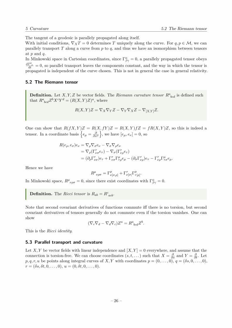
5.2 The Riemann tensor

Definition. Let X,Y, Z be vector fields. The Riemann curvature tensor Rabcd is defined suchthat RabcdZbXcY d = (R(X,Y )Z)a, where

R(X,Y )Z = ∇X∇Y Z −∇Y∇XZ −∇[X,Y ]Z.

One can show that R(fX, Y )Z = R(X, fY )Z = R(X,Y )fZ = fR(X,Y )Z, so this is indeed atensor. In a coordinate basis

eµ = ∂

∂xµ

, we have [eµ, eν ] = 0, so

R(eρ, eσ)eν = ∇ρ∇σeν −∇σ∇ρeν= ∇ρ(Γτνσeτ )−∇σ(Γτνρeτ )= (∂ρΓτνσ)eτ + ΓτνσΓµτρeµ − (∂σΓτνρ)eτ − ΓτνρΓµτσeµ.

Hence we haveRµνρσ = Γµν[σ,ρ] + Γτν[σ|Γ

µτ |ρ].

In Minkowski space, Rµνρσ = 0, since there exist coordinates with Γαβγ = 0.

Definition. The Ricci tensor is Rab = Rcacb.

Note that second covariant derivatives of functions commute iff there is no torsion, but secondcovariant derivatives of tensors generally do not commute even if the torsion vanishes. One canshow

(∇c∇d −∇d∇c)Za = RabcdZb.

This is the Ricci identity.

5.3 Parallel transport and curvatureLet X,Y be vector fields with linear independence and [X,Y ] = 0 everywhere, and assume that theconnection is torsion-free. We can choose coordinates (s, t, . . . ) such that X = ∂

∂s and Y = ∂∂t . Let

p, q, r, u be points along integral curves of X,Y with coordinates p = (0, . . . , 0), q = (δs, 0, . . . , 0),r = (δs, δt, 0, . . . , 0), u = (0, δt, 0, . . . , 0).

– 26 –

5 Curvature 5.4 Symmetries of the Riemann tensor

p

u r

q

Y Y

X

X

Let Zp ∈ Tp(M) be parallely transported along the path described by pqrup to get Z ′p ∈ Tp(M). Itcan be shown that

limδs,δt→0

(Z ′p − Zp)a

δsδt= (RabcdZbY cXd)p.

Thus curvature measures the change of vectors under parallel transport along closed curves.Equivalently: curvature measure the path dependence of parallel transport.

5.4 Symmetries of the Riemann tensorThe first symmetry of the Riemann tensor is self-evident from its definition:

Rabcd = −RabdcNow let the connection be torsion-free and let p ∈M with (xµ) normal coordinates at p.We have Γµνρ = 0 at p, so Rµνρσ = ∂ρΓµνσ − ∂σΓµνρ at p. Antisymmetrising on ν, ρ, σ and usingΓµνρ = 0, we have Rµ[νρσ] = 0 at p. This is a tensorial equation, so it holds in all coordinate systems,and hence

Ra[bcd] = 0 everywhere.

We also have ∇τRµ[νρσ] = ∂τRµνρσ = ∂τ∂ρΓµνσ − ∂τ∂σΓµνρ at p. Antisymmetrising on ρ, σ, τ , we

obtainRµν[ρσ;τ ] = 0 =⇒ Rab[cd;e].

This is the Bianchi identity.

5.5 Geodesic deviationOur goal now is to quantify the relative acceleration of geodesics.

Definition. Let (M,Γ) be a manifold with a connection. A 1-parameter family of geodesics isa map γ : I × I ′ →M where I, I ′ ⊂ R are open, satisfying:

• For fixed s, γ(s, t) is a geodesic with affine parameter t.

• Locally, (s, t) 7→ γ(s, t) is smooth, 1-to-1, and has a smooth inverse.

The family of geodesics forms a 2-dimensional surface Σ ⊂M.

Let T be the tangent to γ(s = constant, t) and S the tangent to γ(s, t = constant). In coordinates(xµ), we have Sµ = ∂xµ

∂s , so we can write

xµ(s+ δs, t) = xµ(s, t) + δsSµ(s, t) +O(δs2).

Hence δsS points from one geodesic to a nearby one; it is known as the deviation vector.

– 27 –

5 Curvature 5.6 Curvature of the Levi-Civita connection

Definition. The relative velocity of nearby geodesics is ∆T (δsS) = δs∇TS.The relative acceleration of nearby geodesics is δs∆T∆TS.

If there is no torsion, the geodesic deviation equation holds:

∆T∆TS = R(T, S)T

Proof. Use coordinates (s, t) on Σ and extend to coordinates (s, t, . . . ) on a neighbourhood of Σ.We have S = ∂

∂s , T = ∂∂t and [S, T ] = 0. Since there is no torsion, we have

∇TS −∇ST = [T, S] = 0 =⇒ ∇T∇TS = ∇T∇ST = ∇S ∇TT︸ ︷︷ ︸=0

+R(T, S)T = R(T, S)T.

Iff Rabcd = 0, then relative acceleration vanishes for all families of geodesics.Tidal forces arise from geodesic deviation.

5.6 Curvature of the Levi-Civita connectionFrom now on, manifolds are assumed to have a metric and the connection is Levi-Civita unlessstated otherwise. Note Rabcd = gaeR

ebcd.

Definition. The Ricci scalar is R = gabRab. The Einstein tensor is Gab = Rab − 12gabR.

Lemma 5. 1. Rabcd = Rcdab ( =⇒ Rbacd = −Rabcd)

2. Rab = Rba

3. ∇aGab = 0 ( contracted Bianchi identity)

Proof. 1. Let p ∈M and use normal coordinates at p. We have ∂ρgµν = 0, so by the chain rulewe have

0 = ∂µδνρ = ∂µ(gνσgσρ) = gσρ∂µg

νσ =⇒ ∂µgντ = 0.

Therefore we have

∂ρΓτnuσ = 12g

τµ(∂ρ∂σgµν + ∂ρ∂νgσµ − ∂ρ∂µgνσ),

and soRµνρσ = 1

2(∂ρ∂νgσµ + ∂σ∂µgνρ − ∂σ∂νgρµ − ∂ρ∂µgνσ) = Rρσµν .

2. Rab = gcdRdacb = gcdRcbda = Rba.

3. This follows from contracting the Bianchi identity and using the above.

– 28 –

6 Diffeomorphisms and Lie derivatives 5.7 Einstein’s equation

5.7 Einstein’s equationWe are now ready to complete the postulates of general relativity. The complete list is as follows:

1. Spacetime is a 4-dimensional Lorentzian manifold with a metric and Levi-Civita connection.

2. Free particles follow timelike or null geodesics.

3. The energy, momentum and stress of matter are described by a symmetric, conserved tensorTab.

4. Curvature is related to matter by the Einstein equations:

Gab = Rab −12gabR = 8πG

c4 Tab

Einstein’s first guess was to set Rab = κTab. Use the contracted Bianchi identity to write

0 = ∇bGab = ∇bRab −12gab∇

bR = ∇bTab︸ ︷︷ ︸=0

−12gab∇

bT.

So ∇bT = 0. But usually T = 0 outside of matter and T 6= 0 inside of matter, so this fails.In a vacuum, Tab = 0 and the Einstein equations are Rab − 1

2gabR = 0. Contracting over ab, we get−R = 0, so the vacuum Einstein equations can simply be written Rab = 0.

Theorem 4 (Lovelock). Let Hab be a symmetric (0, 2) tensor satisfying:

1. For all charts φ we have Hµν = Hµν(gµν , ∂ρgµν , ∂σ∂ρgµν) at all p ∈M.

2. ∇bHab = 0.

3. Hµν is linear in ∂σ∂ρgµν .

Then there exist α, β ∈ R such that Hab = αGab + βgab.

This theorem leads to a modification of the Einstein equation to include a cosmological constant:

Gab + Λgab = 8πTab

We have set G = c = 1.

6 Diffeomorphisms and Lie derivatives6.1 Maps between manifolds

Definition. Let M,N be differentiable manifolds of dimension m,n respectively. A functionφ :M→N is smooth iff ψA φψ−1

α : Rm → Rn is smooth for all charts ψA on N and ψα onM.

Definition. Let φ : M → N , f : N → R be smooth. The pullback of f by φ is the mapφ∗f :M→ R, p 7→ φ∗f(p) = f(φ(p)).

– 29 –

6 Diffeomorphisms and Lie derivatives 6.1 Maps between manifolds

Definition. The pushforward of a curve λ : I →M is φ∗λ = φ λ : I → N , t→ φ(λ(t)).

Definition. Let p ∈M, and let X ∈ Tp(M) be the tangent vector of a curve λ : I →M. Thepushforward of X by φ is φ∗X ∈ Tφ(p)(N ), defined as the tangent of φ∗λ at φ(x).

Lemma 6. Let X ∈ Tp(M) and f : N → R. Then (φ∗X)(f) = X(φ∗f).

Proof. Let λ(0) = p. We have

(φ∗X)(f)|φ(p) =[ d

dt(f (φ λ))(t)]t=0

=[ d

dt((f φ) λ)(t)]t=0

= X(φ∗f).

Definition. Let φ :M→N be smooth, p ∈M and η ∈ T ∗φ(p)(N ). The pullback of η by φ isφ∗η ∈ T ∗p (M), defined by (φ∗η)(X) = η(φ∗X) for all X ∈ Tp(M).

Lemma 7. Let f : N → R. The gradient of f at φ(p) is df ∈ T ∗φ(p)(N ). We have φ∗(df) = d(φ∗f).

Proof. Let X ∈ Tp(M). Then (φ∗(df))(X) = df (φ∗X) = (φ∗X)(f) = X(φ∗f) = [d(φ∗f)](X).

Let xµ be coordinates on M and yα coordinates on N . φ :M→N defines a map xµ 7→ yα(xµ).One can show that for a vector X ∈ Tp(M) we have

(φ∗X)α = ∂yα

∂xµ

∣∣∣∣pXµ,

and for a 1-form η ∈ T ∗P (N ) we have

(φ∗η)µ = ∂yα

∂xµ

∣∣∣∣pηα.

Note that we have not required that φ is invertible, so we only have:

pushforward pullback

functions 7 3

curves 3 7

vectors 3 7

1-forms 7 3

p ∈ M was arbitrary, so the pushforward similarly applies to vector fields and the pullback tocovector fields.We can define the pullback of a (0, s) tensor S by

(φ∗S)(X1, . . . , Xs) = S(φ∗(X1), . . . , φ∗(Xs)) for all X1, . . . , Xs ∈ Tp(M).

Similarly we can define the pushforward of a (r, 0) tensor T by

(φ∗T )(η1, . . . , ηr) = T (φ∗η1, . . . , φ∗ηr) for all η1, . . . , ηr ∈ T ∗p (M).

– 30 –

6 Diffeomorphisms and Lie derivatives 6.2 Diffeomorphisms and diffeomorphism invariance

These have components given by

(φ∗S)µ1...µs = ∂yα1

∂xµ1

∣∣∣∣p. . .

∂yαs

∂xµs

∣∣∣∣pSα1...αs ,

(φ∗T )α1...αr = ∂yα1

∂xµ1

∣∣∣∣p. . .

∂yαr

∂xµr

∣∣∣∣pSµ1...µr .

Example. Let M = S2, N = R3. Use (θ, φ) spherical coordinates on S2 and let φ : M →N , p(θ, φ) 7→ yα = (sin θ cosφ, sin θ sinφ, cos θ). Let g be a Euclidean metric on R3. gαβ = δαβin cartesian coordinates, and the pullback of g onto S2 is (φ∗g)µν = diag(1, sin2 θ).

6.2 Diffeomorphisms and diffeomorphism invariance

Definition. A map φ :M→ N is a diffeomorphism if φ is 1-to-1, onto, smooth, and has asmooth inverse. M and N must have the same dimension.

Definition. Let φ :M→N be a diffemorphism and T a (r, s) tensor onM. The pushforwardof T under φ is the (r, s) tensor on N given by

φ∗T (η1, . . . , ηr, X1, . . . , Xs) = T (φ∗η1, . . . , φ∗ηr, (φ−1)∗X1, . . . , (φ−1)∗Xs)

for all ηi ∈ T ∗φ(p)(N ) and Xi ∈ Tφ(p)(N ). The pullback of S an (r, s) tensor on N is defined tobe φ∗S = (φ−1)∗S.

One can show that the pushforward and pullback commute with contraction and the outer product,and also that the components of the resulting tensor in a coordinate basis are exactly what onewould expect from a coordinate change.There are two viewpoints we can take here. The active viewpoint is that φ : p 7→ φ(p) is a mapbetween two distinct manifolds. The passive viewpoint is that we are pulling back coordinates yµfrom N to M, and so simply have two coordinate charts xµ, yα on M.

Definition. Let φ :M→N be a diffeomorphism, ∇ a covariant derivative on M, X a vectorfield and T a tensor on N . The pushforward of ∇ is the covariant derivative ∇ on N defined by

∇XT = φ∗[∇φ∗X(φ∗T )].

One can show:

• ∇ satisfied the properties of a covariant derivative.

• The Riemann tensor of ∇ is the pushforward of the Riemann tensor of ∇.

• If ∇ is the covariant derivative of the Levi-Civita connection of g on M, then ∇ is thecovariant derivative of the Levi-Civita connection of φ∗g on N .

– 31 –

6 Diffeomorphisms and Lie derivatives 6.3 Lie derivatives, symmetries

We defined a spacetime as a pair (M, g). Now let’s add matter fields F, . . .. Two models (M, g, F, . . . )and (M′, g′, F ′, . . . ) are taken to be equivalent if there exists a diffeomorphism φ :M→M′ whichcarries g, F, . . . to g′, F ′, . . ., i.e. g′ = φ∗g, F ′ = φ∗F , . . .. We have active-passive equivalence,so we can say that the models just differ by a coordinate transformation. Hence a spacetime isreally an equivalence class of equivalent (M, g, F, . . . ). As a consequence, the Einstein equationswill not determine all 10 metric components. Physical statements in general relativity must bediffeomorphism invariant – this is the gauge freedom of general relativity.

Example. The statement “two geodesics intersect at xµ = (. . . )” is not gauge invariant.Consider however a geodesic intersected exactly once by each of two other geodesics. Theproper time between the intersections is gauge invariant.

6.3 Lie derivatives, symmetriesPushforwards and pullbacks enable us to compare tensors at different p, q ∈M.

Definition. A diffeomorphism φ :M→M is a symmetry transformation of a tensor field Tif φ∗T = T everywhere. An isometry is a symmetry transformation of the metric.

Definition. Let X be a vector field on a manifold M. Define φt :M→M, p 7→ q = a pointa parameter distance t along the integral curve of X through p.

For small enough t, φt can be shown to be a diffeomorphism. φ0 is the identity, and we haveφs φt = φs+t, φ−t = (φt)−1. If φt is a diffeomorphism for all t ∈ R, then we can define for allp ∈M the curve λp : R→M, t 7→ φt(p).

Definition. The Lie derivative of a tensor T along a vector field X at p ∈M is

(LXT )p = limt→0

[(φ−t)∗T ]p − Tpt

.

LX maps (r, s) tensor fields to (r, s) tensor fields. If α and β are constants, then we haveLX(αS + βT ) = αLXS + βLXT .

Definition. Let Σ be a (n− 1)-dimensional hypersurface in M, and X be a vector field thatis nowhere tangent to Σ. Let xi, i = 1, . . . , n − 1, be coordinates on Σ. Assign to q ∈ Mcoordinates (t, xi) such that q is a parameter distance t along the integral curve of X throughxi on Σ. For sufficiently small t, (t, xi) is a coordinate chart; these are adapted coordinates.

Note that integral curves of X have fixed xi and parameter t, so we can write X = ∂∂t . The

diffeomorphism φt sends points p with xµ = (tp, xi) to q with yµ = (tp + t, xi), and we have∂yµ

∂xν = δµν . Now consider an (r, s) tensor T in these coordinates. We have

[((φt)∗T )µ...ν...]φt(p) = ∂yµ

∂xρ. . .

∂yσ

∂xν. . . [T ρ...σ... ]p = [Tµ...ν... ]p.

– 32 –

6 Diffeomorphisms and Lie derivatives 6.3 Lie derivatives, symmetries

Hence[((φ±t)∗T )µ...ν...]p = [Tµ...ν... ]φ∓t(p),

and so at p with (tp, xi), in this chart we have

(LXT )µ...ν... = limt→0

1t[Tµ...ν... (tp + t, xi)− Tµ...ν... (tp, xi)] = ∂

∂tTµ...ν... (t, xi)

∣∣∣∣tp

.

It follows that we have a Leibniz rule

LX(S ⊗ T ) = (LXS)⊗ T + S ⊗ (LXT ),

and also that LX commutes with contraction.We still need a chart independent expression. In this chart, LXf = ∂

∂tf for functions f . Also,X(f) = ∂

∂tf . Thus in any basis we have

LXf = X(f).

In our chart, (LXY )µ = ∂Y µ

∂t for a vector field Y . Also, since Xµ = δµ0 , we have [X,Y ]µ = ∂Y µ

∂t .Hence in any basis we have

LXY = [X,Y ].

Note that LXT depends on Xp and its derivatives, so neither L nor LT are tensors. Compare thiswith covariant derivatives, where ∇XT only depends on Xp, so ∇T is a tensor.One can show:

• For a 1-form ω, we have (LXω)µ = Xν∂νωµ + ων∂µXν , so

(LXω)a = Xb∇bωa + ωb∇aXb.

• For tensor T , we have

(LXT )α...β... = Xγ∂γTα...β... − (∂γXα)T γ...β... − · · ·+ (∂βXγ)Tα...γ... + . . . ,

so(LXT )a...b... = Xc∇cT a...b... − (∇cXa)T c...b... − · · ·+ (∇bXc)T a...x... + . . . .

In particular, for the metric, we have

(LXg)µν = Xρ∂ρgµν + gµρ∂νXρ + gρν∂µX

ρ

= gµρ∇νXρ + gρν∇µXρ

= ∇νXµ +∇µXν (for Levi-Civita connection).

Let φt be a continuous family of isometries. For all t ∈ R we have (φt)∗g = g and hence LX(g) = 0,so using the above we obtain

∇aXb +∇bXa = 0;

this is Killing’s equation. Solutions to Killing’s equation are called Killing vector fields.If there exists a chart with one coordinate z on which gµν does not depend, then ∂

∂z is a Killingvector field. Conversely if there is a Killing vector field, then we can choose coordinates such thatgµν does not depend on one of them.

Lemma 8. Let X be a Killing vector field, and let V be a a vector field tangent to an affinelyparametrised geodesic. Then XaV

a is constant along the geodesic.

– 33 –

7 Linearised Theory 7 Linearised Theory

Proof.

ddτ (XaV

a) = V (XaVa) = ∇V (XaV

a) = V b∇b(XaVa)

= V aV b︸ ︷︷ ︸symmetric

antisymmetric︷ ︸︸ ︷∇bXa +Xa V

b∇bBa︸ ︷︷ ︸=0

= 0

One can show that if Tab is the energy-momentum tensor and Xa is a Killing vector field, then thecurrent Ja = T ab is conserve, i.e. ∇aJa = 0.

7 Linearised Theory7.1 The linearised Einstein equationsConsider small deviations from Minkowski spacetime in cartesian coordinates. The “background”spacetime is the manifold M = R4 with metric g = η = diag(−1, 1, 1, 1), and the “perturbation” isa small change to the metric given by h = O(ε) 1 so that g = η + h. We regard hµν as a tensorfield on the background spacetime.We have two metrics, ηµν and gµν . The inverse of gµν is gµν = ηµν − hµν to O(ε). Also to O(ε), itcan be shown that

Γµνρ = 12η

µσ(∂ρhσν + ∂νhσρ − ∂σhνρ) = O(ε).

Hence we have

Rµνρσ = ηµτ (∂ρΓτνσ − ∂σΓτνρ) = 12(∂ρ∂νhµσ + ∂σ∂µhνρ − ∂ρ∂µhνσ − ∂ν∂σhµρ)

=⇒ Rµν = ∂ρ∂(µhν)ρ −12∂

ρ∂ρhµν −12∂µ∂νh

=⇒ Gµν = ∂ρ∂(µhν)ρ −12∂

ρ∂ρhµν −12∂µνh−

12ηµν(∂ρ∂σhρσ − ∂ρ∂ρh) = 8πTµν 1,

where h = hµµ and ∂µ = gµν∂ν .

Definition. The trace-reversed perturbation is hµν = hµν − 12hηµν .

Note that hµν = hµν − 12 h|etaµν , i.e. if we reverse the trace twice we get the original perturbation.

Writing the Einstein tensor in terms of the trace-reversed perturbation simplifies the aboveexpression:

Gµν = −12∂

ρ∂ρhµν + ∂ρ∂(µhν)ρ −12ηµν∂

ρ∂σhρσ

Now let (M, g, T ) be a spacetime, and φ :M→M′ a diffemorphism. Then (M′, φ∗g, φ∗T ) is aphysically equivalent spacetime. We want ηµν to remain the background metric, so we considerφ ∼ O(ε). Consider diffeomorphism φt defined by integral curves of a vector field X. Then t = O(ε).Writing ζµ = tXµ = O(ε), we have for any tensor T

(φ−t)∗(T ) = T + tLXT +O(ε2)= T + LξT +O(ε2).

– 34 –

7 Linearised Theory 7.2 Newtonian limit

The energy momentum tensor is Tµν = O(ε), so ((φ−t)∗T )µν = Tµν +O(ε2). The metric becomes

(φ−t)∗g = g + Lξg + · · · = η + h+ Lξη +O(ε2),

so hµν and hµν + (Lξη)µν are physically equivalent. Hence we have a gauge symmetry

hµν → hµν + ∂µξν + ∂νξµ

=⇒ hµν → hµν + ∂µξν + ∂νξµ − ηµν∂ρξρ

for ξµ = O(ε).Now choose ξµ such that ∂ν∂νξµ = −∂ν hµν . Under this gauge transformation, we have ∂ν hµν → 0(this is the Lorentz gauge), and hence we can choose a gauge so that

Gµν = −12∂

ρ∂ρhµν .

Thus we have the linearised Einstein equations

∂ρ∂ρhµν = −16πTµν .

7.2 Newtonian limitNewtonian gravity can be summarised by ∇2Φ = 4πρ, accurate for Φ ∼ v2 ∼ ε 1. This impliesρ ∼ O(ε), i.e. matter sources are weak. For the energy-momentum tensor, we can write

T00 = ρ+O(ε2),T0i ∼ T00vi ∼ O(ε3/2),Tij ∼ T00vivj ∼ O(ε2).

For example in a perfect fluid with Tµν = (ρ + P )uµuν + Pgµν , we have P ∼ ρv2

c2 , and we havePρ ≈ 10−5 in the sun. In special relativity we have

uµ =(

1√1− v2

,vi√

1− v2

),

where v2 = vivi.In Newtonian gravity, temporal changes in Φ are caused by the motion of sources. Hence we have∂∂t ∼ v ∂

∂xi= O(ε1/2) ∂

∂xi. Therefore hµν = ∂ρ∂ρhµν = ∂i∂ihµν = ∇2hµν = −16πTµν , from which

we deduce that ∇2h00 = −16πρ, h0i = O(ε3/2) and hij = O(ε2). The 00 component is just Newton’slaw with h00 = −4Φ. Thus we have h = ηµν hµν = 4Φ = −h, and so

h00 = h00 −12η00h = −2Φ and hij = −2Φδij .

So in the Newtonian limit, the line element is just

ds2 = −(1 + 2φ) dt2 + (1− 2φ)(dx2 + dy2 + dz2).

Now consider geodesics in the weak field. We have Lagrangian

L = −gµνdxµ

dτdxν

dτ = (1 + 2Φ)t2 − δij(1− 2Φ)xixj = 1.

– 35 –

7 Linearised Theory 7.3 Gravitational waves

Solving for t we havet = (1− Φ) + 1

2δij xixj +O(ε2).

The Euler-Lagrance equation for xk gives

−2δjkxj +O(ε)2 = 2δkΦ.

Combining these two, we getd2xk

dt2 = d2xk

dτ2 = −∂kΦ,

i.e. the equation of motion for a test body in Newtonian theory.

7.3 Gravitational wavesConsider againthe weak field but now in a vacuum, and without the restriction ∂t ∂i. Thevacuum linearised Einstein equations read

hµν = (∂2t −∇2)hµν = 0.

This is just a wave equation, and we have the plane wave solution hµν = Hµνeikµxµ , where Hµν

and kµ are constants. hµν = 0 =⇒ kµkµ = 0, so the wave propagates at the speed of light. In

the Lorentz gauge, ∂ν hµν = 0 =⇒ kµHµν = 0, i.e. oscillations are transverse to the direction ofthe wave. For example if the wave is in the z-direction with kµ = ω(1, 0, 0, 1), then we must haveHµ0 +Hµ3 = 0.Note that in the Lorentz gauge we have some remaining gauge freedom to fix. If we take ξµ =Xµe

ikρxρ , then the Lorentz condition is maintained. Under this transformation we have

Hµν → Hµν + i(kµXν + kνXµ − ηµνkρXρ),

and from this it can be shown that there is a choice of X such that H0µ = 0 and Hµµ = 0. In this

gauge, h = 0 =⇒ hµν = hµν . For a plane wave in the z-direction we have H0µ = H3µ = Hµµ = 0,

so we can write

Hµν =

0 0 0 00 H+ H× 00 H× −H+ 00 0 0 0

for constants H+ and H×.Now consider the effect this wave has on particles. Consider a particle at rest in the backgroundframe with 4-velocity uα(0) = (1, 0, 0, 0). The geodesic equation is

ddtu

α + Γαµν︸︷︷︸O(ε)

uµuν = uα + Γα00 = 0.

Since H0µ = 0, we have Γα00 = 12η

αβ(∂0hβ0 + ∂0h0β − ∂βh00) = 0. Hence uα(τ) = (1, 0, 0, 0), andthe particle stays at xi = constant in this gauge. We are interested in proper separations betweenparticles, so we must use the metric, which is

ds2 = −dt2 + (1 + h+) dx2 + (1− h+) dy2 + 2h× dx dy + dz2 .

First consider the case in which H× = 0 and H+ = 0, so that only h+ oscillates. The properseparation between 2 particles at (±δ, 0, 0) is given by ds2 = (1 + h+)4δ2; similarly for 2 particlesat (0,±δ, 0) we have ds2 + (1− h+)4δ2. Hence the particles move like:

– 36 –

7 Linearised Theory 7.4 The field far from the source

Now consider H× 6= 0, H+ = 0. For 2 particles at (±δ,±δ, 0)/√

2 we have ds2 = (1 + h×)4δ2, andfor 2 particles at (±δ,∓δ, 0)/

√2 we have ds2 = (1− h×)4δ2, so the particles now move like:

7.4 The field far from the sourceConsider a weak field with matter. The linearised equations are ∂ρ∂ρhµν = −16πTµν . By introducinga Green’s function, we can invert this to find

hµν(t,x) = 4∫Tµν(t− |x− y|,y)

|x− y|d3y .

We assume that matter has no compact support inside a radius d, so we can take the integral over|y| < d. We assume we are far from the source, so we take r = |x| d. Hence we can write

|x− y| = r − x · y +O(d/r),

where x = xr . Thus we have

Tµν(t− |x− y|,y) = Tµν(t− r,y)− x · y(∂0Tµν)(t− r,y).

Assuming v c, we have ∂0Tµν ∼ Tµν vd Tµνd , so to leading order we have

hµν(t,x) ≈ 4r

∫Tµν(t− r,y) d3y . (∗)

In the Lorentz gauge, ∂ν hµν = 0 =⇒ ∂0h0i = ∂j hji and ∂0h00 = ∂ih0i. Our strategy will be tocalculate hij → h0i → h00. We have∫

T ij d3y =∫∂k(T ikyj)︸ ︷︷ ︸→0

(surface term)

−(∂kT ik)yj d3y =∫

(∂0Ti0)yj d3y ,

since ∂µT iµ = 0. Thus we can write∫T ij d3y =

∫T (ij) d3y

= ∂0

∫T 0(iyj) d3y

= ∂0

∫ 12 ∂k(T

0kyiyj)︸ ︷︷ ︸→0

−12(∂kT 0k)yiyj d3y

= 12∂0∂0

∫T 00 d3y ,

– 37 –

7 Linearised Theory 7.5 Energy in gravitational waves

so hij = 2r Iij(t− r) where

Iij(t− r) =∫T00(t− r,y)yiyj d3y

is the quadrupole tensor.Next we have

∂0h0i = ∂j hji = ∂j

(2rIij(t− r)

),

so integrating once over t, we have

h0i = ∂j

(2rIij(t− r)

)+ Ci = −2 xj

r2 Iij︸ ︷︷ ︸=O(1/r2)→0

−2 xjrIij + Ci.

We set the constant of integration with (∗), writing

Ci = 4r

∫T0i(0,y) d3y = −4

rPi,

where Pi is the “momentum”. We have

∂0Pi(t− r) = −∫∂0T0i d3y = −

∫∂jTji d3y = 0,

so Pi is conserved at leading order.Finally, to find h00 we use ∂0h00 = ∂ih0i, which similarly gives

h00 = ∂i

(−2xj

rIij(t− r)

)+ C0 = 2 xixj

rIij(t− r) + C0 +O

( 1r2

).

We fix C0 withC0 = 4

r

∫T00(0,Y) d3y = 4

rE,

where E is the energy. We have

∂0E(t− r) = ∂0

∫T00 d3y =

∫∂iTi0 d3y = 0,

so E is conserved to leading order.Note that at higher orders E and Pi are not conserved.

7.5 Energy in gravitational wavesConsider now 2nd order perturbation theory in the vacuum. The notation we will use is

gµν = gµν︸︷︷︸background(typically η)

+ δ(1)gµν︸ ︷︷ ︸firstorder

+ δ(2)gµν︸ ︷︷ ︸secondorder

= ηµν + hµν + h(2)µν .

We use this style of notation for all quantities. To find the inverse to the metric, write

gµν = ηµν + δ(1)gµν + δ(2)gµν .

We havegµρgρν = δµν + hµν + δ(1)gµρηρν︸ ︷︷ ︸

first order

+ δ(2)gµρηρν + h(2)µν + δ(1)gµρhρν︸ ︷︷ ︸

second order

,

– 38 –

7 Linearised Theory 7.5 Energy in gravitational waves

where h(2)µν = ηµρh

(2)ρν . Thus we can deduce

δ(1)gµν = −hµν = g(1)µν [h],δ(2)gµν = −h(2)µν + hµσh ν

σ = g(1)µν [h(2)] + g(2)µν [h].

This is a generic pattern in perturbation theory. Given Sµν a function of the metric, we will obtainfirst and order terms of the form

δ(1)Sµν = S(1)µν [h],δ(2)Sµν = S(1)µν [h(2)] + S(2)µν [h].

Cosnsider the Einstein equations. We have

Gµν = Gµν + δ(1)Gµν + δ(2)Gµν

= 0 +G(1)µν [h] +G(1)

µν [h(2)] +G(2)µν [h],

whereG(2)µν [h] = R(2)

µν [h]− 12R

(1)[h]hµν −12R

(2)[h]ηµν .

As before, since we are in a vacuum, we have G(1)µν [h] = R

(1)µν [h] = 0. The vacuity also allows us to

write G(1)µν [h(2)] = 8πtµν [h], where

tµν [h] = − 18πG

(2)µν [h] = − 1

8π (R(2)µν [h]− 1

2ηρσR(2)

ρσ [h]ηµν).

Consider the contracted Bianchi identities gµρ∇ρgµν = 0. At linear order, these give

∂µG(1)µν [h] = 0 =⇒ ∂µG(1)

µν [h(2)] = 0,

where the implication comes from the fact that the Bianchi identities hold for g = η + h(2). Atquadratic order, making use of Gµν = δ(1)Gµν = 0, they give

∂µ(G(2)µν [h]) = ∂µtµν = 0.

tµν is conserved, like the energy-momentum tensor. In fact, we regard tµν as the energy-momentumof the gravitational field.A problem with this is that tµν is gauge dependent. There are two ways to get around this. Aglobal solution is to integrate over all space, leading to things like the ADM mass (see the BlackHoles course). A local approximation is to use a “large” 4-volume V ∼ a4 as follows.

Definition. The average of a quantity Xµν with respect to a weight function w(x) is

〈Xµν〉 =∫VXµν(x)w(x) d4x .

w(x) must satisfy∫V w(x) d4x = 1 and w(x)→ 0 smoothly on ∂V .

We have〈∂ρXµν〉 =

∫V

(∂ρXµν)w d4x = −∫VXµν(∂ρw) d4x .

– 39 –

8 Differential Forms 7.6 Quadrupole formula

Let Xµν be oscillating with wavelength λ, so that ∂ρXµν ∼ Xµνλ . We also have ∂ρw ∼ W

a . If weassume a λ, then

〈∂ρXµν〉 ∼Xµν

a Xµν

λ∼ ∂ρXµν .

Hence we can neglect total derivatives when taking averages. We can do things like 〈A∂B〉 =〈∂(AB)〉 − 〈(∂A)B〉 ≈ − 〈(∂A)B〉. Using this fact, we find⟨

ηµνR(2)µν [h]

⟩= 0

and〈tµν〉 = 1

32π

⟨∂µhρσ∂ν h

ρσ − 12∂µh∂ν h+ 2∂ρhρσ∂(µhν)σ

⟩.

This expression for 〈tµν〉 is gauge invariant.

7.6 Quadrupole formulaThe energy flux in gravitational waves is given by −〈t0i〉. Consider a sphere far from the sourcewith r d, and let xi = xi

r . The power through the sphere is given by

〈p〉 = −∫r2 〈t0i〉 xi dΩ

where dΩ = sin θ dθ dφ. In the Lorentz gauge ∂ν hνρ = 0, we have

〈t0i〉 = 132π

⟨∂0hρσ∂ih

ρσ − 12∂0h∂ih

⟩.

Using the value for hρσ from before, doing a lot of algebra, and taking things to O(

1r

), we obtain

〈p〉t = 15⟨...Qij

...Qij

⟩t−r

where Qij = Iij −13Ikkδij .

This is the quadrupole formula.

8 Differential Forms8.1 p-forms

Definition. A p-form is a totally antisymmetric tensor of rank (0, p).

0-forms are functions and 1-forms are covectors.

Definition. Let η be a p-form and ω a q-form. Their wedge product η ∧ ω is a (p+ q)-formdefined by

(η ∧ ω)a1...apb1...bq = (p+ q)!p!q! η[a1...apωb1...bq ] ⇐⇒ η ∧ ω = (p+ q)!

p!q! A(η ⊗ ω),

where A is an operator that totally antisymmetrises the given tensor.

– 40 –

8 Differential Forms 8.2 Integration

One can show that η ∧ ω = (−1)pqω ∧ η, so η ∧ η = 0 if p is odd. Also, the wedge product isassociative:

(η ∧ ω) ∧ χ = η ∧ (ω ∧ χ)

Given a dual basis fµ, the p-forms

fµ1 ∧ · · · ∧ fµp = p!(f [µ1 ⊗ · · · ⊗ fµp])

form a basis for the space of p-forms. We will often expand a p-form in terms of its components inthis basis as

η = 1p!ηµ1...µpf

µ1 ∧ · · · ∧ fµp .

Definition. The exterior derivative of a p-form η is a (p+ 1)-form dη given by

(dη)µ1...µp+1 = (p+ 1)∂(µ1)ηµ2...µp+1] = (p+ 1)[∇[µ1ηµ2...µp+1 + Γρ[µ2µ1︸ ︷︷ ︸

=0(torsion free)

η|ρ|µ3...µp+1

]

It can be shown that:

• d(dη) = 0.

• d(η ∧ ω) = dη ∧ ω + (−1)pη ∧ dω (η a p-form).

• d(φ∗η) = φ∗ dη.

Definition. A p-form η is closed if dη = 0, and exact if there exists a (p− 1)-form ω such thatη = dω.

Note that if η is exact, then it is closed. The converse is not always true, but we do have:

Lemma 9 (Poincare lemma). If η is closed, then for all points r ∈M there exists a neighbourhoodO of r and a (p− 1)-form ω such that η = dω in O.

In other words, if η is closed, then it is locally exact.

8.2 Integration

Lemma 10. Let ω be a n-form and fµ a dual basis for an n-dimensional manifold M. Thenthere exists a function h such that ω = hf1 ∧ . . . fn.

Definition. An orientation of an n-dimensional manifold N is a smooth nowhere vanishingn-form η, up to an equivalence given by η ∼ η′ iff there exists a function h > 0 such thatη′ = hη.

Definition. A coordinate chart xµ on N is right-handed relative to a given orientation η ifthere exists a function h > 0 such that η = hdx1 ∧ · · · ∧ dxµ.

– 41 –

8 Differential Forms 8.3 Submanifolds, Stokes’ theorem

Definition. The volume form on (N , g) is ε =√|g|f1 ∧ · · · ∧ fn, where g = detgαβ.

Definition. Let ψ = xµ : O ⊂ N → Rn be a right-handed coordinate chart, and ω a n-form.Then the integral of ω over O is∫

Oω =

∫ψ(O)⊂Rn

ω1...n dx1 . . . dxn .

To integrate over regions with more than one chart, we add these expressions patchwise.

This expression for the integral can be shown to be chart independent. We can integrate a functionf using the volume form: ∫

Ofε =

∫ψ(O)

f√|g| dx1 . . . dxn

Definition. A diffeomorphism φ : N → N is orientation preserving if φ∗η is equivalent to ηfor all orientations η.

If φ is orientation preserving, it can be shown that∫N φ∗ω =

∫N ω.

8.3 Submanifolds, Stokes’ theoremLet M,N be orientable manifolds of dimensions m < n.

Definition. An embedding φ :M→N is a smooth, 1-to-1 map such that for all p ∈M thereexists a neighbourhood O such that φ−1 : φ(O)→M is smooth. If m = n− 1, then φ(M) is ahypersurface.

Definition. Let φ[M] be m-dimensional, and let η be an m-form on N . Then we define theintegral of η over φ[M] as ∫

φ[M]η =

∫Mφ∗η.

Note that if η = dω then we have ∫φ[M]

dω =∫M

dφ∗η .

Definition. Let 12R

n = (x1, . . . , xn) ∈ R s. t. x1 ≤ 0. A manifold with boundary N isidentical to a manifold, except for that the charts now map to 1

2Rn. Its boundary is ∂N = p ∈

N s. t. x1(p) = 0, and is (n−1)-dimensional. (x2, . . . , xn) is right-handed on ∂N if (x1, . . . , xn)is right-handed on ∂M.

Theorem 5 (Stokes’ theorem). Given an n-dimensional orientable manifold N with boundary ∂Nand (n− 1)-form η, we have ∫

Ndη =

∫∂N

η.

– 42 –

9 The Initial Value Problem 9 The Initial Value Problem

Definition. X ∈ Tp(N ) is tangent to φ(M) if there exists a curve in φ(M) with tangent X.n ∈ T ∗p (N ) is normal to φ(M) if n(X) = 0 for all X tangent to φ(M.

Definition. Let Σ be a hypersurface of a Lorentzian manifold with normal field n. Σ isspacelike (timelike, null) if n is timelike (spacelike, null). On ∂N , dx1 is the outgoing normalto ∂N .

Theorem 6 (Divergence theorem). Let ∂N be timelike or spacelike, X a vector field on N , andhµν = φ∗gµν for φ : ∂N → N , p 7→ p. Then we have∫

N∇aXa

√|g| dnx =

∫naX

a√|h| dn−1x .

9 The Initial Value Problem9.1 Extrinsic curvatureLet N be a manifold, Σ a hypersurface, and g the metric (Riemannian or Lorentzian). The unitnormal to Σ is the normal n such that nana = ∓1. We take the upper sign if n is timelike, and thelower sign if n is spacelike.

Definition. The projector onto Σ is ⊥ab= δab ± nanb. Given a tensor T , its projection ⊥ Tonto Σ is given by

⊥ T ab...cd... =⊥ae⊥bf · · · ⊥gc⊥hd . . . Tef...

gh... .

We have:• ⊥ab nb = 0 and ⊥ac⊥cb=⊥ab, so this is indeed a projection operator.

• For all X ∈ Tp(N ), we have that ⊥ab Xb is tangent to Σ, and we can write

Xa =⊥ab Xb ∓ nanbXb.

• Given X,Y tangent to Σ, we have gabXaY b =⊥ab XaY a. For this reason, ⊥ab is often

called the induced metric on Σ, and we write γab =⊥ab. It is also sometimes called the 1stfundamental form.

Let X,Y be tangent vector fields to Σ, and N some normal vector field. Parallely transport Nalong the integral curves of X so that Xb∇bNa = 0. Does N remain normal to Σ? Not in general.We have

Xb∇b(Y aNa) = NaXb∇bY a 6= 0 in general.

Thus we have another kind of curvature for Σ.

Definition. Extend the unit normal n is a neighbourhood of Σ, maintaining nana = ∓1. Theextrinsic curvature of Σ is the (0, 2) tensor

K : Tp(N )× Tp(N ) → RX,Y 7→ na(∇⊥X(⊥ Y ))a .

– 43 –

9 The Initial Value Problem 9.2 The Gauss-Codazzi equations

Note that we have made a choice of sign convention here.

Lemma 11. Kab = − ⊥ca⊥ db∇cnd and is independent of the extension of n.

Proof. First we prove the expression. We have

KabXaY b = na(⊥ X)c∇c(⊥ Y )a

= −(⊥ X)c(⊥ Y )a∇cna= − ⊥cb Xb ⊥ad Y d∇cna

=⇒ Kbd = − ⊥cb⊥ad ∇cna.

Now we prove that it is independent of the extension of n. Consider another extension n′a and letma = n′a − na, which vanishes on Σ. On Σ, we have

XaY b(Kab −K ′ab) =⊥ca⊥db XaY b∇cmd

= (⊥ X)c[(⊥ Y )d∇cmd + md︸︷︷︸

=0

∇c(⊥ Y )d]

= (⊥ X)c∇c(md(⊥ Y )d) = 0.

Note that we have nb∇cnb = 12∇c(nbn

b) = 0, so we can write

Kab = − ⊥ca⊥db ∇cnd = − ⊥ca (δdb ± ndnb)∇cnd = − ⊥ca ∇cnb.

Definition. Let t : N → R with t = constant and dt 6= 0 on Σ. Then we can write the unitnormal as n = ∓α dt, where

α = 1±√g−1(dt ,dt)

is the lapse. The choice of sign means that n is future pointing if it is timelike.

Lemma 12. Kab = Kba.

Proof. We have∇cnd = ∓∇c(α(dt)d) = ∓α∇c∇dt+ (∇cα)nd

α,

so Kab = ± ⊥ca⊥db α∇c∇dt, which is symmetric (for vanishing torsion).

Definition. K = Kbb = gabKab =⊥ab Kab = γabKab.

9.2 The Gauss-Codazzi equations

Definition. The covariant derivative Da on Σ is defined by

DaTb...c... =⊥da⊥be · · · ⊥fc . . .∇dT e...f ... .

– 44 –

9 The Initial Value Problem 9.3 The constraint equations

It can be shown that D is torsion free and the Levi-Civita connection of γab on Σ if ∇ is that ofgab on N . D defines the Riemann tensor of γab, which we write as Rabcd. One can calculate theprojections of Rabcd using the Ricci identity. We obtain:

Gauss equation : ⊥ Rabcd = Rabcd ± 2Ka[cKd]b.

Contracted Gauss : ⊥ Rab± ⊥ca nd ⊥eb nfRcdef = Rab ±KKab ∓KacKcb .

Scalar Gauss : R± 2Rcdncnd = R±K2 ∓KcdKcd.

Codazzi : ⊥da⊥eb⊥fc ngRdefg = −DaKbc +DbKac.

Contracted Codazzi : ⊥cb Rcdnd = −DaKab +DbK.

9.3 The constraint equationsFrom now on we will take n timelike (so we use the upper sign). We wish to project the Einsteinequations Gab = 8πTab onto Σ. From the energy-momentum tensor we define

ρ = Rabnanb, ja = − ⊥ba Tbcnc, Sab =⊥ Tab.

Contracting the Einstein equations with nanb, we have Rabnanb + 12R = 8πρ, and if we substitute

in the scalar Gauss equation, we obtain

R−KcdKcd +K2 − 16πρ = 0.

This is the Hamiltonian constraint.If we contract with na and then project with ⊥, we get ⊥ba ncRbc = −8πja. Substituting in thecontracted Codazzi equation, we have

DcKca −DaK − 8πja = 0.

This is the momentum constraint.

9.4 Foliations

Definition. A Cauchy surface is a spacelike hypersurface Σ in N such that each timelike ornull curve without endpoints intersects Σ exactly once. (N , g) is globally hyperbolic if it admitsa Cauchy surface.

From now on we assume that (N , g) is globally hyperbolic. One can show that this implies thatthere is a smooth t : N → R such that dt 6= 0 everywhere, and the hypersurfaces Σ are levelsurfaces with t = constant. Thus for all t ∈ R we have a surface Σt = p ∈ N s. t. t(p) = t, andΣt ∩ Σt′ 6= ∅ ⇐⇒ t = t′. We assume that the Σt are spacelike, and that N =

⋃t∈R Σt. Such a

family of hypersurfaces is called a foliation of N . From now on we will just use t without referringto t.

Definition. m = αn is the normal evolution vector.

– 45 –

9 The Initial Value Problem 9.5 The 3 + 1 equations

Since n = −α dt and n · n = −1, we have m ·m = −α2 and 〈dt ,m〉 = − 1α 〈n,m〉 = 1. Using this

we see that Lmt = m(t) = 〈dt ,m〉 = 1, so the proper time along integral curves of m is given by

τ =∫ t

t0

√−g(m,m) dt =⇒ dτ

dt =√−g(m,m) = α.

Definition. The acceleration is ab = nc∇cnb.

Lemma 13. ab = Db logα.

Recall that Kab = − ⊥ca ∇cnb = −∇anb − nanc∇cnb, so we can write

∇anb = −Kab − naab = −Kab − naDb logα.

Hence we have

∇amb = ∇a(αnb) = nb∇aα+ α∇anb = nb∇aα− αKab − naDbα.

Lemma 14. • Lmγab = −2αKab.

• Lnγab = −2Kab.

• Lmγab = Lm ⊥ab= 0.

• Lnγab = naDb logα.

Corollary. Let T be a tangent tensor, i.e. ⊥ T = T . Then we have

LmT = Lm(⊥ T ) = (Lm ⊥)︸ ︷︷ ︸=0

T+ ⊥ LmT =⊥ LmT,

so LmT is also tangent to Σ.

With these tools we can calculate the final projection. A lot of effort gives

⊥ea⊥gbn

hRefghnf = 1

αLmKab +KacK

cb + 1

αDaDbα.

With the contracted Gauss equation we have

⊥ Rab = − 1αLmKab −

1αDaDbα+Rab +KKab − 2KacK

cb .

Finally, contracting with ⊥ab and using the scalar Gauss equation, we have

R = 2αLmK −

2αDcD

cα+R+K2 +KcdKcd.

9.5 The 3 + 1 equationsThe Einstein equations can be written as Rab = 8π(Tab − 1

2gabT ). Projecting this, we obtain

⊥ Rab = 4π(2Sab + (ρ− S)γab).

Using the results of the last section, we find

LmKab = −DaDbα+ α Rab +KKab − 2KacKcb + 4π[(S − ρ)γab − 2Sab] .

Now we need to relate Lm to a time deriative ∂∂t . We use adapated coordinates xα = (t, xi),

i = 1, 2, 3, where xi label points in σt. This gives a basis ∂t, ∂i and a corresponding dual basisdt ,dxi. Integral curves of the ∂i have t = constant, so they are in one σt. What about integralcurves of ∂t? Clearly 〈dt , ∂t〉 = 1 = 〈dt ,m〉, so 〈dt , ∂t −m〉 = 0.

– 46 –

10 The Lagrangian Formulation

Definition. The shift vector is β = ∂t −m.

We have 〈dt , β〉 = 0, and we can write ∂t = αn+ β. Curves with xi constant are not in generalnormal to Σt, and β measures this deviation.Using the definitions of α and β, we obtain that the components of the metric are

gαβ =(−α2 + βkβ

k βjβi γij

)⇐⇒ gαβ =

(−α−2 α−2βjα−2βi γij − α−2βiβj

).

Hence we have det gαβ = −α2 det γij , so√−g = α

√γ.

In adapted coordinates, the 3 + 1 equations contain only tensors tangent to Σt, so we can ignoretime components and substitute i, j, · · · = 1, 2, 3 for abstract indices. We have

Lmγij = L∂tγij − Lβγij = ∂

∂tγij − βm∂mγij − γmj∂iβm − γim∂jβm

andLmKij = ∂

∂tKij − βm∂mKij −Kmj∂iβ

m −Kim∂jβj .

Hence we have:

∂tγij = Lβγij − 2αKij

∂tKij = LβKij −DiDjααRij +KKij − 2KimK

mj + 4π[(S − ρ)γij − 2Sij ]

Together with the constraint equations this is our full set of equations.Note that α, βi are freely specifiable, reflecting gauge freedom. Also, it can be shown from theBianchi identities that the constraints are preserved under time evolution.

10 The Lagrangian FormulationConsider a scalar field in a curved spacetime. The action is

S =∫M

[−1

2gαβ∇αφ∇βφ− V (φ)

]√−g d4x .

If we vary with respect to φ and assume δφ vanishes on ∂M, we find

δS = S[φ+ δφ]− S[φ]

=∫M

[−gαβ∇αφ∇βδφ− V ′(φ)δφ

]√−g d4x

=∫M

[−∇α(δφ∇αφ) + δφ∇α∇αφ− V ′(φ)δφ

]√−g d4x

=∫∂M−δφnα∇αφ

√|h|︸ ︷︷ ︸

=0

+∫M

(∇α∇αφ− V ′(φ))δφ√−g d4x .

Setting the variation equal to zero we get the equation of motion

∇α∇α − V ′(φ) = 0.

– 47 –

10 The Lagrangian Formulation

We would like to be able to do the same thing, but with an action that replicates general relativity.We will take the following sign conventions: the unit normal n is always outgoing, and the extrinsiccurvature is Kab = + ⊥ ∇anb. Consider a region in a manifold V. Then the action for that regionis given by:

SGR[g, φ] = 116π (IH [g] + IB[g]− I0) + SM [φ, g]

Here φ represents all matter fields.There are several terms in this action which we will explore one by one:

1. IH =∫V R√−g d4x is the Hilbert term.

2. IB = 2∮∂V K

√|γ|d3y is the boundary term (γ =⊥ g).

3. I0 = 2∮∂V K0

√|γ|d3y is the constant term.

4. SM =∫V L(φ, φ,α; gαβ)

√−g d4x is the matter term.

We will be varying gαβ and it is convenient to note the following:

gαµgµβ = δαβ =⇒ δgαβ = −gαµgβνδgµν

Also:

Lemma 15. δ√−g = −1

2√−ggαβδgαβ.

Consider first the Hilbert term. We have

δIH =∫Vδ(gαβRαβ

√−g d4x

=∫VRαβ√−gδgαβ + gαβ

√−gδRαβ +Rδ

√−g d4x

=∫V

(Rαβ −12Rgαβ)︸ ︷︷ ︸

=Gαβ

δgαβ√−g d4x+

∫VgαβδRαβ

√−g d4x .

In normal coordinates, we have

∂Rαβ = δ(Γµαβ,µ − Γµαµ,β) = δΓµαβ;µ − δΓµαµ;β.

Recall that δΓ is a tensor, so this is a tensorial equation and is thus valid in all coordinates. Hence∫VgαβδRαβ

√−g d4x =

∫VXµ

;µ√−g d4x =

∮∂VXµnµ

√|γ|d3y ,

where Xµ = gαβδΓµαβ − gαµδΓβαβ. On ∂V, we have δgαβ = δgαβ = 0, so δΓµαβ = 1

2gµν(δgνα,β +

δgνβ,α + δgαβ,ν). From this it can be shown that

Xµ = gµν gαβ(δgνα,β − δgαβ,ν)︸ ︷︷ ︸=Xν

.

Hence we have

nµXµ = nµ (γαβ ∓ nαnβ)︸ ︷︷ ︸=gαβ

(δgµβ,α − δgαβ,µ)︸ ︷︷ ︸antisymmetric in µ, α

= nµγαβ(δgµβ,α − δgαβ,µ).

– 48 –

10 The Lagrangian Formulation

The first term is the part of the derivative of δgµβ tangent to ∂V, and so vanishes. Substitutingthis into the above we obtain:

δIH =∫VGαβδg

αβ√−g d4x−∮∂Vγαβδgαβ,µn

µ√|γ| d3y (∗)

Now look at the boundary term. We have K = γαβKαβ = γαβ∇αnβ = γαβ(∂αnβ − Γµβαnµ). Hence

δK = −γαβδΓµαβnµ

= −12γ

αβ(δgµα,β + δgµβ,α − δgαβ,µ)nµ

= 12γ

αβδgαβ,µnµ

=⇒ δIB =∮∂Vγαβδgαβ,µn

µ√|γ|d3y .

Behold: the second term in (∗) is cancelled.The constant term I0 depends on gαβ only through

√|γ|, so we automatically have δI0 = 0 on ∂V.

Thus I0 has no effect on the equations of motion. What it does do is regularise the value of SGR.To demonstrate, let gαβ be a solution of the vacuum equations Rαβ = R = 0. Then

SGR + 116πI0 = 1

16πIB = 18π

∮∂VK|γ|

12 d3y .

Evaluate this on a closed 3-cylinder of radius R for a flat spacetime. On Σt1 and Σt2 , we haveK = 0. At r = R, we can show that K = 2

R . We also have |γ|12 = R2 sin θ. Hence we have∮

∂V|γ|

12 d3y = 8πR(t2 − t1),

which diverges as R→∞. This divergence persists in curved spacetimes. Therefore we use I0 tocancel this divergence, with K0 = the curvature of ∂V embedded in flat spacetime.The variation of the matter term is

δSM =∫V

∂L

∂gαβδgαβ

√−g + Lδ

√−g d4x =

∫V

(∂L

∂gαβ− 1

2Lgαβ)δgαβ

√−g d4x .

This leads to the following

Definition. Tαβ = −2 ∂L∂gαβ

+ Lgαβ is the energy-momentum tensor.

With this definition we have ∂SM = −12∫V Tαβδg

αβ√−g d4x.So the total variation of the action is

δSGR =∫V

(Gαβ − 8πTαβ)δgαβ√−g d4x .

Thus if we enforce δSGR = 0, we recover the Einstein equations:

Gαβ = 8πTαβ

Fin

– 49 –