gaussian random vectors and processes
TRANSCRIPT

Chapter 3
GAUSSIAN RANDOMVECTORS AND PROCESSES
3.1 Introduction
Poisson processes and Gaussian processes are similar in terms of their simplicity and beauty.When we first look at a new problem involving stochastic processes, we often start withinsights from Poisson and/or Gaussian processes. Problems where queueing is a majorfactor tend to rely heavily on an understanding of Poisson processes, and those where noiseis a major factor tend to rely heavily on Gaussian processes.
Poisson and Gaussian processes share the characteristic that the results arising from themare so simple, well known, and powerful that people often forget how much the resultsdepend on assumptions that are rarely satisfied perfectly in practice. At the same time,these assumptions are often approximately satisfied, so the results, if used with insight andcare, are often useful.
This chapter is aimed primarily at Gaussian processes, but starts with a study of Gaussian(normal1) random variables and vectors, These initial topics are both important in theirown right and also essential to an understanding of Gaussian processes. The material hereis essentially independent of that on Poisson processes in Chapter 2.
3.2 Gaussian random variables
A random variable (rv) W is defined to be a normalized Gaussian rv if it has the density
fW (w) =1p2⇡
exp✓�w2
2
◆; for all w 2 R. (3.1)
1Gaussian rv’s are often called normal rv’s. I prefer Gaussian, first because the corresponding processesare usually called Gaussian, second because Gaussian rv’s (which have arbitrary means and variances) areoften normalized to zero mean and unit variance, and third, because calling them normal gives the falseimpression that other rv’s are abnormal.
109

110 CHAPTER 3. GAUSSIAN RANDOM VECTORS AND PROCESSES
Exercise 3.1 shows that fW (w) integrates to 1 (i.e., it is a probability density), and that Whas mean 0 and variance 1.
If we scale a normalized Gaussian rv W by a positive constant �, i.e., if we consider therv Z = �W , then the distribution functions of Z and W are related by FZ(�w) = FW (w).This means that the probability densities are related by �fZ(�w) = fW (w). Thus the PDFof Z is given by
fZ(z) =1�
fW⇣ z
�
⌘=
1p2⇡ �
exp✓�z2
2�2
◆. (3.2)
Thus the PDF for Z is scaled horizontally by the factor �, and then scaled vertically by1/� (see Figure 3.1). This scaling leaves the integral of the density unchanged with value 1and scales the variance by �2. If we let � approach 0, this density approaches an impulse,i.e., Z becomes the atomic rv for which Pr{Z=0} = 1. For convenience in what follows, weuse (3.2) as the density for Z for all � � 0, with the above understanding about the � = 0case. A rv with the density in (3.2), for any � � 0, is defined to be a zero-mean Gaussianrv. The values Pr{|Z| > �} = .318, Pr{|Z| > 3�} = .0027, and Pr{|Z| > 5�} = 2.2 · 10�12
give us a sense of how small the tails of the Gaussian distribution are.
fW (w)
fZ(w)
0 2 4 6
0.3989
Figure 3.1: Graph of the PDF of a normalized Gaussian rv W (the taller curve) andof a zero-mean Gaussian rv Z with standard deviation 2 (the flatter curve).
If we shift Z by an arbitrary µ 2 R to U = Z+µ, then the density shifts so as to be centeredat E [U ] = µ, and the density satisfies fU (u) = fZ(u� µ). Thus
fU (u) =1p2⇡ �
exp✓�(u� µ)2
2�2
◆. (3.3)
A random variable U with this density, for arbitrary µ and � � 0, is defined to be a Gaussianrandom variable and is denoted U ⇠ N (µ,�2).
The added generality of a mean often obscures formulas; we usually assume zero-mean rv’sand random vectors (rv’s) and add means later if necessary. Recall that any rv U with amean µ can be regarded as a constant µ plus the fluctuation, U � µ, of U .
The moment generating function, gZ(r), of a Gaussian rv Z ⇠ N (0,�2), can be calculated

3.3. GAUSSIAN RANDOM VECTORS 111
as follows:
gZ(r) = E [exp(rZ)] =1p2⇡ �
Z 1
�1exp(rz) exp
�z2
2�2
�dz
=1p2⇡ �
Z 1
�1exp
�z2 + 2�2rz � r2�4
2�2+
r2�2
2
�dz (3.4)
= expr2�2
2
�⇢1p2⇡ �
Z 1
�1exp
�(z � r�)2
2�2
�dz
�(3.5)
= expr2�2
2
�. (3.6)
We completed the square in the exponent in (3.4). We then recognized that the term inbraces in (3.5) is the integral of a probability density and thus equal to 1.
Note that gZ(r) exists for all real r, although it increases rapidly with |r|. As shown inExercise 3.2, the moments for Z ⇠ N (0,�2), can be calculated from the MGF to be
EhZ2k
i=
(2k)!�2k
k! 2k= (2k � 1)(2k � 3)(2k � 5) . . . (3)(1)�2k. (3.7)
Thus, E⇥Z4
⇤= 3�4, E
⇥Z6
⇤= 15�6, etc. The odd moments of Z are all zero since z2k+1 is
an odd function of z and the Gaussian density is even.
For an arbitrary Gaussian rv U ⇠ N (µ,�2), let Z = U � µ, Then Z ⇠ N (0,�2) and gU (r)is given by
gU (r) = E [exp(r(µ + Z))] = erµE⇥erZ
⇤= exp(rµ + r2�2/2). (3.8)
The characteristic function, gZ(i✓) = E⇥ei✓Z
⇤for Z ⇠ N (0,�2) and i✓ imaginary can be
shown to be (e.g., see Chap. 2.12 in [27]).
gZ(i✓) = exp�✓2�2
2
�, (3.9)
The argument in (3.4) to (3.6) does not show this since the term in braces in (3.5) isnot a probability density for r imaginary. As explained in Section 1.5.5, the characteristicfunction is useful first because it exists for all rv’s and second because an inversion formula(essentially the Fourier transform) exists to uniquely find the distribution of a rv from itscharacteristic function.
3.3 Gaussian random vectors
An n ⇥ ` matrix [A] is an array of n` elements arranged in n rows and ` columns; Ajk
denotes the kth element in the jth row. Unless specified to the contrary, the elements arereal numbers. The transpose [AT] of an n⇥` matrix [A] is an `⇥n matrix [B] with Bkj = Ajk

112 CHAPTER 3. GAUSSIAN RANDOM VECTORS AND PROCESSES
for all j, k. A matrix is square if n = ` and a square matrix [A] is symmetric if [A] = [A]T.If [A] and [B] are each n⇥ ` matrices, [A]+ [B] is an n⇥ ` matrix [C] with Cjk = Ajk +Bjk
for all j, k. If [A] is n ⇥ ` and [B] is ` ⇥ r, the matrix [A][B] is an n ⇥ r matrix [C] withelements Cjk =
Pi AjiBik. A vector (or column vector) of dimension n is an n by 1 matrix
and a row vector of dimension n is a 1 by n matrix. Since the transpose of a vector is arow vector, we denote a vector a as (a1, . . . , an)T. Note that if a is a (column) vector ofdimension n, then aaT is an n⇥n matrix whereas aTa is a number. The reader is expectedto be familiar with these vector and matrix manipulations.
The covariance matrix, [K] (if it exists) of an arbitrary zero-mean n-rv Z = (Z1, . . . , Zn)T
is the matrix whose components are Kjk = E [ZjZk]. For a non-zero-mean n-rv U , letU = m + Z where m = E [U ] and Z = U �m is the fluctuation of U . The covariancematrix [K] of U is defined to be the same as the covariance matrix of the fluctuation Z ,i.e., Kjk = E [ZjZk] = E [(Uj �mj)(Uk �mk)]. It can be seen that if an n ⇥ n covariancematrix [K] exists, it must be symmetric, i.e., it must satisfy Kjk = Kkj for 1 j, k n.
3.3.1 Generating functions of Gaussian random vectors
The moment generating function (MGF) of an n-rv Z is defined as gZ (r) = E [exp(rTZ )]where r = (r1, . . . , rn)T is an n-dimensional real vector. The n-dimensional MGF mightnot exist for all r (just as the one-dimensional MGF discussed in Section 1.5.5 need notexist everywhere). As we will soon see, however, the MGF exists everywhere for Gaussiann-rv’s.
The characteristic function, gZ (i✓✓✓) = Ehei✓✓✓TZ
i, of an n-rv Z , where ✓✓✓ = (✓1, . . . , ✓n)T is
a real n-vector, is equally important. As in the one-dimensional case, the characteristicfunction always exists for all real ✓✓✓ and all n-rv Z . In addition, there is a uniquenesstheorem2 stating that the characteristic function of an n-rv Z uniquely specifies the jointdistribution of Z .
If the components of an n-rv are independent and identically distributed (IID), we call thevector an IID n-rv.
3.3.2 IID normalized Gaussian random vectors
An example that will become familiar is that of an IID n-rvW where each component Wj ,1 j n, is normalized Gaussian, Wj ⇠ N (0, 1). By taking the product of n densities asgiven in (3.1), the joint density of W = (W1,W2, . . . ,Wn)T is
fW (w) =1
(2⇡)n/2exp
✓�w2
1 � w22 � · · ·� w2
n
2
◆=
1(2⇡)n/2
exp✓�wTw
2
◆. (3.10)
2See Shiryaev, [27], for a proof in the one-dimensional case and an exercise providing the extension tothe n-dimensional case. It appears that the exercise is a relatively straightforward extension of the prooffor one dimension, but the one-dimensional proof is measure theoretic and by no means trivial. The readercan get an engineering understanding of this uniqueness theorem by viewing the characteristic function andjoint probability density essentially as n-dimensional Fourier transforms of each other.

3.3. GAUSSIAN RANDOM VECTORS 113
The joint density of W at a sample value w depends only on the squared distance wTw ofthe sample value w from the origin. That is, fW (w) is spherically symmetric around theorigin, and points of equal probability density lie on concentric spheres around the origin(see Figure 3.2).
&%'$
n w1
w2
Figure 3.2: Equi-probability contours for an IID Gaussian 2-rv.
The moment generating function of W is easily calculated as follows:
gW (r) = E [exp rTW )] = E [exp(r1W1 + · · · + rnWn] = E
24Y
j
exp(rjWj)
35
=Yj
E [exp(rjWj)] =Yj
exp
r2j
2
!= exp
rTr
2
�. (3.11)
The interchange of the expectation with the product above is justified because, first, therv’s Wj (and thus the rv’s exp(rjWj)) are independent, and, second, the expectation of aproduct of independent rv’s is equal to the product of the expected values. The MGF ofeach Wj then follows from (3.6). The characteristic function of W is similarly calculatedusing (3.9),
gW (i✓✓✓) = exp�✓✓✓T✓✓✓
2
�, (3.12)
Next consider rv’s that are linear combinations of W1, . . . ,Wn, i.e., rv’s of the form Z =aTW = a1W1 + · · · + anWn. By convolving the densities of the components ajWj , itis shown in Exercise 3.4 that Z is Gaussian, Z ⇠ N (0,�2) where �2 =
Pnj=1 a2
j , i.e.,Z ⇠ N (0,
Pj a2
j ).
3.3.3 Jointly-Gaussian random vectors
We now go on to define the general class of zero-mean jointly-Gaussian n-rv’s.
Definition 3.3.1. {Z1, Z2, . . . , Zn} is a set of jointly-Gaussian zero-mean rv’s, and Z =(Z1, . . . , Zn)T is a Gaussian zero-mean n-rv, if, for some finite set of IID N (0, 1) rv’s,

114 CHAPTER 3. GAUSSIAN RANDOM VECTORS AND PROCESSES
W1, . . . ,Wm, each Zj can be expressed as
Zj =mX
`=1
aj`W` i.e., Z = [A]W (3.13)
where {aj`, 1 j n, 1 ` m, } is a given array of real numbers. More generally,U = (U1, . . . , Un)T is a Gaussian n-rv if U = Z + µµµ, where Z is a zero-mean Gaussiann-rv and µµµ is a real n vector.
We already saw that each linear combination of IID N (0, 1) rv’s is Gaussian. This definitiondefines Z1, . . . , Zn to be jointly Gaussian if all of them are linear combinations of a commonset of IID normalized Gaussian rv’s. This definition might not appear to restrict jointly-Gaussian rv’s far beyond being individually Gaussian, but several examples later show thatbeing jointly Gaussian in fact implies a great deal more than being individually Gaussian.We will also see that the remarkable properties of jointly Gaussian rv’s depend very heavilyon this linearity property.
Note from the definition that a Gaussian n-rv is a vector whose components are jointlyGaussian rather than only individually Gaussian. When we define Gaussian processes later,the requirement that the components be jointly Gaussian will again be present.
The intuition behind jointly-Gaussian rv’s is that in many physical situations there aremultiple rv’s each of which is a linear combination of a common large set of small essen-tially independent rv’s. The central limit theorem indicates that each such sum can beapproximated by a Gaussian rv, and, more to the point here, linear combinations of thosesums are also approximately Gaussian. For example, when a broadband noise waveformis passed through a narrowband linear filter, the output at any given time is usually wellapproximated as the sum of a large set of essentially independent rv’s. The outputs at dif-ferent times are di↵erent linear combinations of the same set of underlying small, essentiallyindependent, rv’s. Thus we would expect a set of outputs at di↵erent times to be jointlyGaussian according to the above definition.
The following simple theorem begins the process of specifying the properties of jointly-Gaussian rv’s. These results are given for zero-mean rv’s since the extension to non-zeromean is obvious.
Theorem 3.3.1. Let Z = (Z1, . . . , Zn)T be a zero-mean Gaussian n-rv. Let Y = (Y1, . . . , Yk)T
be a k-rv satisfying Y = [B]Z. Then Y is a zero-mean Gaussian k-rv.
Proof: Since Z is a zero-mean Gaussian n-rv, it can be represented as Z = [A]W wherethe components of W are IID and N (0, 1). Thus Y = [B][A]W . Since [B][A] is a matrix,Y is a zero-mean Gaussian k-rv.
For k = 1, this becomes the trivial but important corollary:
Corollary 3.3.1. Let Z = (Z1, . . . , Zn)T be a zero-mean Gaussian n-rv. Then for any realn-vector a = (a1, . . . , an)T, the linear combination aTZ is a zero-mean Gaussian rv.

3.3. GAUSSIAN RANDOM VECTORS 115
We next give an example of two rv’s, Z1, Z2 that are each zero-mean Gaussian but for whichZ1 + Z2 is not Gaussian. From the theorem, then, Z1 and Z2 are not jointly Gaussian andthe 2-rv Z = (Z1, Z2)T is not a Gaussian vector. This is the first of a number of laterexamples of rv’s that are marginally Gaussian but not jointly Gaussian.
Example 3.3.1. Let Z1 ⇠ N (0, 1), and let X be independent of Z1 and take equiprobablevalues ±1. Let Z2 = Z1X1. Then Z2 ⇠ N (0, 1) and E [Z1Z2] = 0. The joint probabilitydensity, fZ1Z2(z1, z2), however, is impulsive on the diagonals where z2 = ±z1 and is zeroelsewhere. Then Z1 +Z2 can not be Gaussian, since it takes on the value 0 with probabilityone half.
This example also shows the falseness of the frequently heard statement that uncorrelatedGaussian rv’s are independent. The correct statement, as we see later, is that uncorrelatedjointly Gaussian rv’s are independent.
The next theorem specifies the moment generating function (MGF) of an arbitrary zero-mean Gaussian n-rv Z . The important feature is that the MGF depends only on thecovariance function [K]. Essentially, as developed later, Z is characterized by a probabilitydensity that depends only on [K].
Theorem 3.3.2. Let Z be a zero-mean Gaussian n-rv with covariance matrix [K]. Thenthe MGF, gZ(r) = E [exp(rTZ)] and the characteristic function gZ(i✓✓✓) = E [exp(i✓✓✓TZ)] aregiven by
gZ(r) = exprT[K] r
2
�; gZ(i✓✓✓) = exp
�✓✓✓T[K]✓✓✓
2
�. (3.14)
Proof: For any given real n-vector r = (r1, . . . , rn)T, let X = rTZ . Then from Corollary3.3.1, X is zero-mean Gaussian and from (3.6),
gX(s) = E [exp(sX)] = exp(�2Xs2/2). (3.15)
Thus for the given r ,
gZ (r) = E [exp(rTZ )] = E [exp(X)] = exp(�2X/2), (3.16)
where the last step uses (3.15) with s = 1. Finally, since X = rTZ , we have
�2X = E
⇥|rTZ |2
⇤= E [rTZZ Tr ] = rTE [ZZ T] r = rT[K]r . (3.17)
Substituting (3.17) into (3.16), yields (3.14). The proof is the same for the characteristicfunction except (3.9) is used in place of (3.6).
Since the characteristic function of an n-rv uniquely specifies the CDF, this theorem alsoshows that the joint CDF of a zero-mean Gaussian n-rv is completely determined by thecovariance function. To make this story complete, we will show later that for any possiblecovariance function for any n-rv, there is a corresponding zero-mean Gaussian n-rv withthat covariance.

116 CHAPTER 3. GAUSSIAN RANDOM VECTORS AND PROCESSES
As a slight generaliization of (3.14), let U be a Gaussian n-rv with an arbitrary mean, i.e.,U = m + Z where the n-vector m is the mean of U and the zero-mean Gaussian n-rv Zis the fluctuation of U . Note that the covariance matrix [K] of U is the same as that forZ , yielding
gU (r) = exp✓rTm +
rT[K] r2
◆; gU (i✓✓✓) = exp
i✓✓✓Tm � ✓✓✓T[K]✓✓✓
2
�. (3.18)
We denote a Gaussian n-rv U of mean m and covariance [K] as U ⇠ N (m , [K]).
3.3.4 Joint probability density for Gaussian n-rv’s (special case)
A zero-mean Gaussian n-rv, by definition, has the form Z = [A]W where W is N (0, [In]).In this section we look at the special case where [A] is n⇥n and non-singular. The covariancematrix of Z is then
[K] = E [ZZ T] = E [[A]WW T[A]T]
= [A]E [WW T] [A]T = [A][A]T (3.19)
since E [WW T] is the identity matrix, [In].
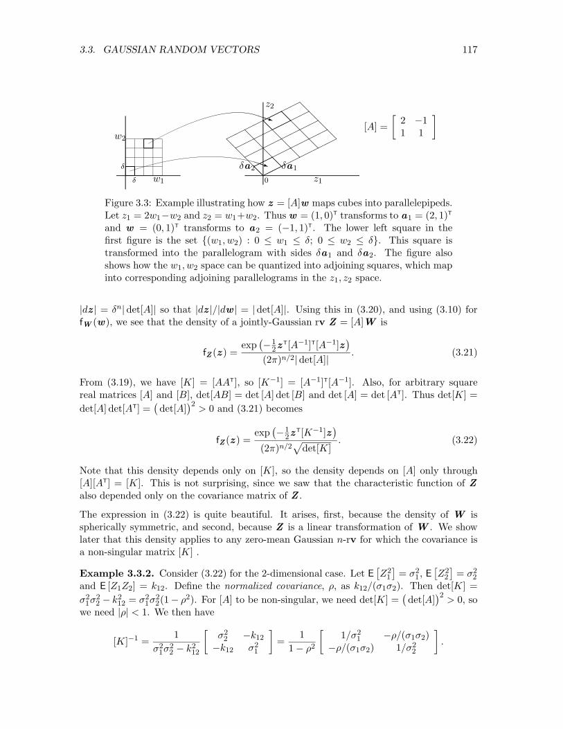
To find fZ (z ) in this case, we first consider the transformation of real-valued vectors, z =[A]w . Let ej be the jth unit vector (i.e., the vector whose jth component is 1 and whoseother components are 0). Then [A]ej = aj , where aj is the jth column of [A]. Thus,z = [A]w transforms each unit vector ej into the column aj of [A]. For n=2, Figure 3.3shows how this transformation carries each vector w into the vector z = [A]w . Note thatan incremental square, � on a side is carried into an parallelogram with corners 0 ,a1�,a2�,and (a1 + a2)�.
For an arbitrary number of dimensions, the unit cube in the w space is the set of points{w : 0 wj 1; 1 j n} There are 2n corners of the unit cube, and each is some0/1 combination of the unit vectors, i.e., each has the form ej1 + ej2 + · · · + ejk . Thetransformation [A]w carries the unit cube into a parallelepiped, where each corner of thecube, ej1 +ej2 + · · ·+ejk , is carried into a corresponding corner aj1 +aj2 + · · ·+ajn of theparallelepiped. One of the most interesting and geometrically meaningful properties of thedeterminant, det[A], of a square real matrix [A] is that the magnitude of that determinant,|det[A]|, is equal to the volume of that parallelepiped (see Strang, [28]). If det[A] = 0, i.e.,if [A] is singular, then the n-dimensional unit cube in the w space is transformed into alower-dimensional parallelepiped whose volume (as a region of n-dimensional space) is 0.This case is considered in Section 3.4.4.
Now let z be a sample value of Z , and let w = [A]�1z be the corresponding sample valueof W . The joint density at z must satisfy
fZ (z)|dz | = fW (w)|dw |, (3.20)
where |dw | is the volume of an incremental cube with dimension � = dwj on each side,and |dz | is the volume of that incremental cube transformed by [A]. Thus |dw | = �n and
3.3. GAUSSIAN RANDOM VECTORS 117
[A] =
2 �11 1
��
�@
@�
�
0�
�
w1
w2
z1
z2
PPq�
��
��
��
�
��
��
��
��
��
��
��
��
��
��
��
��
��
��
��
��
@@
@@
@@
@@
@@
@@
@@
@@
@@
@@
��
@�a2 �a1@�
�
PPq
Figure 3.3: Example illustrating how z = [A]w maps cubes into parallelepipeds.Let z1 = 2w1�w2 and z2 = w1+w2. Thus w = (1, 0)T transforms to a1 = (2, 1)T
and w = (0, 1)T transforms to a2 = (�1, 1)T. The lower left square in thefirst figure is the set {(w1, w2) : 0 w1 �; 0 w2 �}. This square istransformed into the parallelogram with sides �a1 and �a2. The figure alsoshows how the w1, w2 space can be quantized into adjoining squares, which mapinto corresponding adjoining parallelograms in the z1, z2 space.
|dz | = �n|det[A]| so that |dz |/|dw | = |det[A]|. Using this in (3.20), and using (3.10) forfW (w), we see that the density of a jointly-Gaussian rv Z = [A]W is
fZ (z ) =exp
��1
2zT[A�1]T[A�1]z
�(2⇡)n/2|det[A]| . (3.21)
From (3.19), we have [K] = [AAT], so [K�1] = [A�1]T[A�1]. Also, for arbitrary squarereal matrices [A] and [B], det[AB] = det [A] det [B] and det [A] = det [AT]. Thus det[K] =det[A] det[AT] =
�det[A]
�2> 0 and (3.21) becomes
fZ (z ) =exp
��1
2zT[K�1]z
�(2⇡)n/2
pdet[K]
. (3.22)
Note that this density depends only on [K], so the density depends on [A] only through[A][AT] = [K]. This is not surprising, since we saw that the characteristic function of Zalso depended only on the covariance matrix of Z .
The expression in (3.22) is quite beautiful. It arises, first, because the density of W isspherically symmetric, and second, because Z is a linear transformation of W . We showlater that this density applies to any zero-mean Gaussian n-rv for which the covariance isa non-singular matrix [K] .
Example 3.3.2. Consider (3.22) for the 2-dimensional case. Let E⇥Z2
1
⇤= �2
1, E⇥Z2
2
⇤= �2
2and E [Z1Z2] = k12. Define the normalized covariance, ⇢, as k12/(�1�2). Then det[K] =�2
1�22 � k2
12 = �21�
22(1� ⇢2). For [A] to be non-singular, we need det[K] =
�det[A]
�2> 0, so
we need |⇢| < 1. We then have
[K]�1 =1
�21�
22 � k2
12
�2
2 �k12
�k12 �21
�=
11� ⇢2
1/�2
1 �⇢/(�1�2)�⇢/(�1�2) 1/�2
2
�.

118 CHAPTER 3. GAUSSIAN RANDOM VECTORS AND PROCESSES
fZ (z ) =1
2⇡p
�21�
22 � k2
12
exp✓�z2
1�22 + 2z1z2k12 � z2
2�21
2(�21�
22 � k2
12)
◆
=1
2⇡�1�2
p1�⇢2
exp
0@�
z21
�21
+ 2⇢z1z2�1�2
� z22
�22
2(1� ⇢2)
1A . (3.23)
The exponent in (3.23) is a quadratic in z1, z2 and from this it can be deduced that theequiprobability contours for Z are concentric ellipses. This will become clearer (both forn = 2 and n > 2) in Section 3.4.4.
Perhaps the more important lesson from (3.23), however, is that vector notation simplifiessuch equations considerably even for n = 2. We must learn to reason directly from thevector equations and use standard computer programs for required calculations.
For completeness, let U = µµµ + Z where µµµ = E [U ] and Z is a zero-mean Gaussian n-rvwith the density in (3.21). Then the density of U is given by
fU (u) =exp
��1
2(u �µµµ)T[K�1](u �µµµ)�
(2⇡)n/2p
det[K], (3.24)
where [K] is the covariance matrix of both U and Z .
3.4 Properties of covariance matrices
In this section, we summarize some simple properties of covariance matrices that will be usedfrequently in what follows. We start with symmetric matrices before considering covariancematrices.
3.4.1 Symmetric matrices
A number � is said to be an eigenvalue of an n ⇥ n matrix, [B], if there is a non-zeron-vector q such that [B]q = �q , i.e., such that [B � �I]q = 0. In other words, � is aneigenvalue of [B] if [B � �I] is singular. We are interested only in real matrices here, butthe eigenvalues and eigenvectors might be complex. The values of � that are eigenvaluesof [B] are the solutions to the characteristic equation, det[B � �I] = 0, i.e., they are theroots of det[B � �I]. As a function of �, det[B � �I] is a polynomial of degree n. Fromthe fundamental theorem of algebra, it therefore has n roots (possibly complex and notnecessarily distinct).
If [B] is symmetric, then the eigenvalues are all real.3 Also, the eigenvectors can all bechosen to be real. In addition, eigenvectors of distinct eigenvalues must be orthogonal, andif an eigenvalue � has multiplicity ` (i.e., det[B � �I] as a polynomial in � has an `th orderroot at �), then ` orthogonal eigenvectors can be chosen for that �.
3See Strang [28] or other linear algebra texts for a derivation of these standard results.

3.4. PROPERTIES OF COVARIANCE MATRICES 119
What this means is that we can list the eigenvalues as �1,�2, . . . ,�n (where each distincteigenvalue is repeated according to its multiplicity). To each eigenvalue �j , we can asso-ciate an eigenvector q j where q1, . . . , qn are orthogonal. Finally, each eigenvector can benormalized so that q j
Tqk = �jk where �jk = 1 for j = k and �jk = 0 otherwise; the set{q1, . . . , qn} is then called orthonormal.
If we take the resulting n equations, [B]q j = �jq j and combine them into a matrix equation,we get
[BQ] = [Q⇤], (3.25)
where [Q] is the n ⇥ n matrix whose columns are the orthonormal vectors q1, . . . qn andwhere [⇤] is the n⇥ n diagonal matrix whose diagonal elements are �1, . . . ,�n.
The matrix [Q] is called an orthonormal or orthogonal matrix and, as we have seen, hasthe property that its columns are orthonormal. The matrix [Q]T then has the rows qT
jfor 1 j n. If we multiply [Q]T by [Q], we see that the j, k element of the productis q j
Tqk = �jk. Thus [QTQ] = [I] and [QT] is the inverse, [Q�1], of [Q]. Finally, since[QQ�1] = [I] = [QQT], we see that the rows of Q are also orthonormal. This can besummarized in the following theorem:
Theorem 3.4.1. Let [B] be a real symmetric matrix and let [⇤] be the diagonal ma-trix whose diagonal elements �1, . . . ,�n are the eigenvalues of [B], repeated according tomultiplicity.. Then a set of orthonormal eigenvectors q1, . . . , qn can be chosen so that[B]qj = �jqj for 1 j n. The matrix [Q] with orthonormal columns q1, . . . , qn satisfies(3.25). Also [QT] = [Q�1] and the rows of [Q] are orthonormal. Finally [B] and [Q] satisfy
[B] = [Q⇤Q�1]; [Q�1] = [QT] (3.26)
Proof: The only new statement is the initial part of (3.26), which follows from (3.25) bypost-multiplying both sides by [Q�1].
3.4.2 Positive definite matrices and covariance matrices
Definition 3.4.1. A real n ⇥ n matrix [K] is positive definite if it is symmetric and ifbT[K]b > 0 for all real n-vectors b 6= 0. It is positive semi-definite4 if bT[K]b � 0. It is acovariance matrix if there is a zero-mean n-rv Z such that [K] = E [ZZT].
We will see shortly that the class of positive semi-definite matrices is the same as the class ofcovariance matrices and that the class of positive definite matrices is the same as the classof non-singular covariance matrices. First we develop some useful properties of positive(semi-) definite matrices.
4Positive semi-definite is sometimes referred to as nonnegative definite, which is more transparent butless common.

120 CHAPTER 3. GAUSSIAN RANDOM VECTORS AND PROCESSES
Theorem 3.4.2. A symmetric matrix [K] is positive definite5 if and only if each eigenvalueof [K] is positive. It is positive semi-definite if and only if each eigenvalue is nonnegative.
Proof: Assume that [K] is positive definite. It is symmetric by the definition of positivedefiniteness, so for each eigenvalue �j of [K], we can select a real normalized eigenvector q j
as a vector b in Definition 3.4.1. Then
0 < qTj [K]q j = �jq
Tjq j = �j ,
so each eigenvalue is positive. To go the other way, assume that each �j > 0 and use theexpansion of (3.26) with [Q�1] = [QT]. Then for any real b 6= 0,
bT[K]b = bT[Q⇤QT]b = cT[⇤]c where c = [QT]b.
Now [⇤]c is a vector with components �jcj . Thus cT[⇤]c =P
j �jc2j . Since each cj is real,
c2j � 0 and thus c2
j�j � 0. Since c 6= 0, cj 6= 0 for at least one j and thus �jc2j > 0 for at
least one j, so cT[⇤]c > 0. The proof for the positive semi-definite case follows by replacingthe strict inequalitites above with non-strict inequalities.
Theorem 3.4.3. If [K] = [AAT] for some real n⇥n matrix [A], then [K] is positive semi-definite. If [A] is also non-singular, then [K] is positive definite.
Proof: For the hypothesized [A] and any real n-vector b,
bT[K]b = bT[AAT]b = cTc � 0 where c = [AT]b.
Thus [K] is positive semi-definite. If [A] is non-singular, then c 6= 0 if b 6= 0. Thus cTc > 0for b 6= 0 and [K] is positive definite.
A converse can be established showing that if [K] is positive (semi-)definite, then an [A]exists such that [K] = [A][AT]. It seems more productive, however, to actually specify amatrix with this property.
From (3.26) and Theorem 3.4.2, we have
[K] = [Q⇤Q�1]
where, for [K] positive semi-definite, each element �j on the diagonal matrix [⇤] is nonneg-ative. Now define [⇤1/2] as the diagonal matrix with the elements
p�j . We then have
[K] = [Q⇤1/2⇤1/2Q�1] = [Q⇤1/2Q�1][Q⇤1/2Q�1]. (3.27)
Define the square-root matrix [R] for [K] as
[R] = [Q⇤1/2Q�1]. (3.28)
5Do not confuse the positive definite and positive semi-definite matrices here with the positive andnonnegative matrices we soon study as the stochastic matrices of Markov chains. The terms positive definiteand semi-definite relate to the eigenvalues of symmetric matrices, whereas the terms positive and nonnegativematrices relate to the elements of typically non-symmetric matrices.

3.4. PROPERTIES OF COVARIANCE MATRICES 121
Comparing (3.27) with (3.28), we see that [K] = [R R]. However, since [Q�1] = [QT], wesee that [R] is symmetric and consequently [R] = [RT]. Thus
[K] = [RRT], (3.29)
and [R] is one choice for the desired matrix [A]. If [K] is positive definite, then each �j > 0so each
p�j > 0 and [R] is non-singular. This then provides a converse to Theorem 3.4.3,
using the square-root matrix for [A]. We can also use the square root matrix in the followingsimple theorem:
Theorem 3.4.4. Let [K] be an n ⇥ n semi-definite matrix and let [R] be its square-rootmatrix. Then [K] is the covariance matrix of the Gaussian zero-mean n-rv Y = [R]Wwhere W ⇠ N (0, [In]).
Proof:
E [YY T] = [R]E [WW T] [RT] = [R RT] = [K].
We can now finally relate covariance matrices to positive (semi-) definite matrices.
Theorem 3.4.5. An n⇥n real matrix [K] is a covariance matrix if and only if it is positivesemi-definite. It is a non-singular covariance matrix if and only if it is positive definite.
Proof: First assume [K] is a covariance matrix, i.e., assume there is a zero-mean n-rv Zsuch that [K] = E [ZZ T]. For any given real n-vector b, let the zero-mean rv X satisfyX = bTZ . Then
0 E⇥X2
⇤= E [bTZZ Tb] = bTE [ZZ T] b = bT[K]b.
Since b is arbitrary, this shows that [K] is positive semi-definite. If in addition, [K] isnon-singular, then it’s eigenvalues are all non-zero and thus positive. Consequently [K] ispositive definite.
Conversely, if [K] is positive semi-definite, Theorem 3.4.4 shows that [K] is a covariancematrix. If, in addition, [K] is positive definite, then [K] is non-singular and [K] is then anon-singular covariance matrix.
3.4.3 Joint probability density for Gaussian n-rv’s (general case)
Recall that the joint probability density for a Gaussian n-rv Z was derived in Section 3.3.4only for the special case where Z = [A]W where the n⇥ n matrix [A] is non-singular andW ⇠ N (0, [In]). The above theorem lets us generalize this as follows:
Theorem 3.4.6. Let a Gaussian zero-mean n-rv Z have a non-singular covariance matrix[K]. Then the probability density of Z is given by (3.22).

122 CHAPTER 3. GAUSSIAN RANDOM VECTORS AND PROCESSES
Proof: Let [R] be the square root matrix of [K] as given in (3.28). From Theorem 3.4.4,the Gaussian vector Y = [R]W has covariance [K]. Also [K] is positive definite, so fromTheorem 3.4.3 [R] is non-singular. Thus Y satisfies the conditions under which (3.22) wasderived, so Y has the probability density in (3.22). Since Y and Z have the same covarianceand are both Gaussian zero-mean n-rv’s, they have the same characteristic function, andthus the same distribution.
The question still remains about the distribution of a zero-mean Gaussian n-rv Z with asingular covariance matrix [K]. In this case [K�1] does not exist and thus the density in(3.22) has no meaning. From Theorem 3.4.4, Y = [R]W has covariance [K] but [R] issingular. This means that the individual sample vectors w are mapped into a proper linearsubspace of Rn. The n-rv Z has zero probability outside of that subspace and, viewed asan n-dimensional density, is impulsive within that subspace.
In this case [R] has one or more linearly dependent combinations of rows. As a result, one ormore components Zj of Z can be expressed as a linear combination of the other components.Very messy notation can then be avoided by viewing a maximal linearly-independent set ofcomponents of Z as a vector Z 0. All other components of Z are linear combinations of Z 0.Thus Z 0 has a non-singular covariance matrix and its probability density is given by (3.22).
Jointly-Gaussian rv’s are often defined as rv’s all of whose linear combinations are Gaussian.The next theorem shows that this definition is equivalent to the one we have given.
Theorem 3.4.7. Let Z1, . . . , Zn be zero-mean rv’s. These rv’s are jointly Gaussian if andonly if
Pnj=1 ajZj is zero-mean Gaussian for all real a1, . . . , an.
Proof: First assume that Z1, . . . , Zn are zero-mean jointly Gaussian, i.e., Z = (Z1, . . . , Zn)T
is a zero-mean Gaussian n-rv. Corollary 3.3.1 then says that aTZ is zero-mean Gaussianfor all real a = (a1, . . . , an)T.
Second assume that for all real vectors ✓✓✓ = (✓1, . . . , ✓n)T, ✓✓✓TZ is zero-mean Gaussian.For any given ✓✓✓, let X = ✓✓✓TZ , from which it follows that �2
X = ✓✓✓T[K]✓✓✓, where [K] isthe covariance matrix of Z . By assumption, X is zero-mean Gaussian, so from (3.9), thecharacteristic function, gX(i�) = E [exp(i�X], of X is
gX(i�) = exp✓��2�2
X
2
◆= exp
✓��2✓✓✓T[K]✓✓✓
2
◆(3.30)
Setting � = 1, we see that
gX(i) = E [exp(iX)] = E [exp(i✓✓✓TZ )] .
In other words, the characteristic function of X = ✓✓✓TZ , evaluated at � = 1, is the charac-teristic function of Z evaluated at the given ✓✓✓. Since this applies for all choices of ✓✓✓,
gZ (i✓✓✓) = exp✓�✓✓✓T[K]✓✓✓
2
◆(3.31)
From (3.14), this is the characteristic function of an arbitrary Z ⇠ N (0, [K]). Since thecharacteristic function uniquely specifies the distribution of Z , we have shown that Z is azero-mean Gaussian n-rv.

3.4. PROPERTIES OF COVARIANCE MATRICES 123
The following theorem summarizes the conditions under which a set of zero-mean rv’s arejointly Gaussian
Theorem 3.4.8. The following four sets of conditions are each necessary and su�cient fora zero-mean n-rv Z to be a zero-mean Gaussian n-rv, i.e., for the components Z1, . . . , Zn
of Z to be jointly Gaussian:
• Z can be expressed as Z = [A]W where [A] is real and W is N (0, [I]).
• For all real n-vectors a, the rv aTZ is zero-mean Gaussian.
• The linearly independent components of Z have the probability density in (3.22).
• The characteristic function of Z is given by (3.9).
We emphasize once more that the distribution of a zero-mean Gaussian n-rv depends only onthe covariance, and for every covariance matrix, zero-mean Gaussian n-rv’s exist with thatcovariance. If that covariance matrix is diagonal (i.e., the components of the Gaussian n-rvare uncorrelated), then the components are also independent. As we have seen from severalexamples, this depends on the definition of a Gaussian n-rv as having jointly-Gaussiancomponents.
3.4.4 Geometry and principal axes for Gaussian densities
The purpose of this section is to explain the geometry of the probability density contoursof a zero-mean Gaussian n-rv with a non-singular covariance matrix [K]. From (3.22), thedensity is constant over the region of vectors z for which z T[K�1]z = c for any given c > 0.We shall see that this region is an ellipsoid centered on 0 and that the ellipsoids for di↵erentc are concentric and expanding with increasing c.
First consider a simple special case where Z1, . . . , Zn are independent with di↵erent vari-ances, i.e., Zj ⇠ N (0,�j) where �j = E
hZ2
j
i. Then [K] is diagonal with elements �1, . . . ,�n
and [K�1] is diagonal with elements ��11 , . . . ,��1
n . Then the contour for a given c is
z T[K�1]z =nX
j=1
z2j �
�1j = c. (3.32)
This is the equation of an ellipsoid which is centered at the origin and has axes lined upwith the coordinate axes. We can view this ellipsoid as a deformed n-dimensional spherewhere the original sphere has been expanded or contracted along each coordinate axis j bya linear factor of
p�j . An example is given in Figure 3.4.
For the general case with Z ⇠ N (0, [K]), the equiprobability contours are similar, exceptthat the axes of the ellipsoid become the eigenvectors of [K]. To see this, we represent [K]as [Q⇤QT] where the orthonormal columns of [Q] are the eigenvectors of [K] and [⇤] is the

124 CHAPTER 3. GAUSSIAN RANDOM VECTORS AND PROCESSES
i
j
z1
z2cp
�1
cp
�2
Figure 3.4: A contour of equal probability density for 2 dimensions with diagonal [K].The figure assumes that �1 = 4�2. The figure also shows how the joint probabilitydensity can be changed without changing the Gaussian marginal probability densitities.For any rectangle aligned with the coordinate axes, incremental squares can be placedat the vertices of the rectangle and ✏ probability can be transferred from left to right ontop and right to left on bottom with no change in the marginals. This transfer can bedone simultaneously for any number of rectangles, and by reversing the direction of thetransfers appropriately, zero covariance can be maintained. Thus the elliptical contourproperty depends critically on the variables being jointly Gaussian rather than merelyindividually Gaussian.
diagonal matrix of eigenvalues, all of which are positive. Thus we want to find the set ofvectors z for which
z T[K�1]z = z T[Q⇤�1QT]z = c. (3.33)
Since the eigenvectors q1, . . . , qn are orthonormal, they span Rn and any vector z 2 Rn
can be represented as a linear combination, sayP
j vjq j of q1, . . . , qn. In vector termsthis is z = [Q]v . Thus v represents z in the coordinate basis in which the axes are theeigenvectors q1, . . . , qn. Substituting z = [Q]v in (3.33),
z T[K�1]z = vT[⇤�1]v =nX
j=1
v2j �
�1j = c. (3.34)
This is the same as (3.32) except that here the ellipsoid is defined in terms of the represen-tation vj = qT
jz for 1 j n. Thus the equiprobability contours are ellipsoids whose axesare the eigenfunctions of [K]. (see Figure 3.5). We can also substitute this into (3.22) toobtain what is often a more convenient expression for the probability density of Z .
fZ (z ) =exp
⇣�1
2
Pnj=1 v2
j ��1j
⌘(2⇡)n/2
pdet[K]
(3.35)
=nY
j=1
exp(�v2j /(2�j)p
2⇡�j, (3.36)
where vj = qTjz and we have used the fact that det[K] =
Qj �j .

3.5. CONDITIONAL PDF’S FOR GAUSSIAN RANDOM VECTORS 125
⌘⌘
⌘⌘
⌘⌘3
⌘⌘3
JJ
JJ]
JJJ]
cp
�1q1cp
�2q2
q1q2
Figure 3.5: Contours of equal probability density. Points z on the q j axis arepoints for which vk = 0 for all k 6= j. Points on the illustrated ellipse satisfyz T[K�1]z = c.
3.5 Conditional PDF’s for Gaussian random vectors
Next consider the conditional probability fX|Y (x|y) for two zero-mean jointly-Gaussian ran-dom vectors X and Y with a non-singular covariance matrix. From (3.23),
fX,Y (x, y) =1
2⇡�X�Y
p1� ⇢2
exp�(x/�X)2 + 2⇢(x/�X)(y/�Y )� (y/�Y )2
2(1� ⇢2)
�,
where ⇢ = E [XY ] /(�X�Y ). Since fY (y) = (2⇡�2Y )�1/2 exp(�y2/2�2
Y ), we have
fX|Y (x|y) =1
�X
p2⇡(1� ⇢2)
exp�(x/�X)2 + 2⇢(x/�X)(y/�Y )� ⇢2(y/�Y )2
2(1� ⇢2)
�.
The numerator of the exponent is the negative of the square (x/�x � ⇢y/�y)2. Thus
fX|Y (x|y) =1
�X
p2⇡(1� ⇢2)
exp
"� [x� ⇢(�X/�Y )y]2
2�2X(1� ⇢2)
#. (3.37)
This says that, given any particular sample value y for the rv Y , the conditional density ofX is Gaussian with variance �2
X(1�⇢2) and mean ⇢(�X/�Y )y. Given Y =y, we can view Xas a random variable in the restricted sample space where Y =y. In that restricted samplespace, X is N
�⇢(�X/�Y )y, �2
X(1� ⇢2)�.
We see that the variance of X, given Y = y, has been reduced by a factor of 1�⇢2 from thevariance before the observation. It is not surprising that this reduction is large when |⇢| isclose to 1 and negligible when ⇢ is close to 0. It is surprising that this conditional varianceis the same for all values of y. It is also surprising that the conditional mean of X is linearin y and that the conditional distribution is Gaussian with a variance constant in y.
Another way to interpret this conditional distribution of X conditional on Y is to use theabove observation that the conditional fluctuation of X, conditional on Y = y, does not

126 CHAPTER 3. GAUSSIAN RANDOM VECTORS AND PROCESSES
depend on y. This fluctuation can then be denoted as a rv V that is independent of Y .Thus we can represent X as X = ⇢(�X/�Y )Y + V where V ⇠ N (0, (1 � ⇢2)�2
X) and V isindependent of Y .
As will be seen in Chapter 10, this simple form for the conditional distribution leads toimportant simplifications in estimating X from Y . We now go on to show that this samekind of simplification occurs when we study the conditional density of one Gaussian randomvector conditional on another Gaussian random vector, assuming that all the variables arejointly Gaussian.
Let X = (X1, . . . ,Xn)T and Y = (Y1, . . . , Ym)T be zero-mean jointly Gaussian rv’s oflength n and m (i.e., X1, . . . ,Xn, Y1, . . . , Ym are jointly Gaussian). Let their covariancematrices be [KX ] and [KY ] respectively. Let [K] be the covariance matrix of the (n+m)-rv(X1, . . . ,Xn, Y1, . . . , Ym)T.
The (n+m) ⇥ (n+m) covariance matrix [K] can be partitioned into n rows on top and mrows on bottom, and then further partitioned into n and m columns, yielding:
[K] =
24 [KX ] [KX ·Y ]
[KTX ·Y ] [KY ]
35 . (3.38)
Here [KX ] = E [XX T], [KX ·Y ] = E [XY T], and [KY ] = E [YY T]. Note that if X and Y
have means, then [KX ] = Eh(X �X )(X �X )T
i, [KX ·Y ] = E
h(X �X )(Y �Y )T
i, etc.
In what follows, assume that [K] is non-singular. We then say that X and Y are jointlynon-singular, which implies that none of the rv’s X1, . . . ,Xn, Y1, . . . , Ym can be expressedas a linear combination of the others. The inverse of [K] then exists and can be denoted inblock form as
[K�1] =
24 [B] [C]
[CT] [D]
35 . (3.39)
The blocks [B], [C], [D] can be calculated directly from [KK�1] = [I] (see Exercise 3.16),but for now we simply use them to find fX |Y (x |y).
We shall find that for any given y , fX |Y (x |y) is a jointly-Gaussian density with a conditionalcovariance matrix equal to [B�1] (Exercise 3.11 shows that [B] is non-singular). As in(3.37), where X and Y are one-dimensional, this covariance does not depend on y . Also,the conditional mean of X , given Y = y , will turn out to be �[B�1C]y . More precisely,we have the following theorem:
Theorem 3.5.1. Let X and Y be zero-mean, jointly Gaussian, jointly non-singular rv’s.Then X, conditional on Y = y, is N
�� [B�1C]y , [B�1]
�, i.e.,
fX|Y(x|y) =exp
n�1
2
⇣x + [B�1C]yT
⌘[B]
⇣x + [B�1C]y
⌘o(2⇡)n/2
pdet[B�1]
. (3.40)

3.5. CONDITIONAL PDF’S FOR GAUSSIAN RANDOM VECTORS 127
Proof: Express fX |Y (x |y) as fXY (x ,y)/fY (y). From (3.22),
fXY (x ,y) =exp
��1
2(x T,yT)[K�1](x T,yT)T
(2⇡)(n+m)/2p
det[K�1]
=exp
��1
2 (x T[B]x + x T[C]y + yT[CT]x + yT[D]y)
(2⇡)(n+m)/2p
det[K�1].
Note that x appears only in the first three terms of the exponent above, and that x doesnot appear at all in fY (y). Thus we can express the dependence on x in fX |Y (x |y) by
fX |Y (x | y) = �(y) exp⇢�1
2
hx T[B]x + x T[C]y + yT[CT]x
i�, (3.41)
where �(y) is some function of y . We now complete the square around [B] in the exponentabove, getting
fX |Y (x | y) = �(y) exp⇢�1
2
h(x +[B�1C]y)T[B] (x +[B�1C]y) + yT[CTB�1C]y
i�.
Since the last term in the exponent does not depend on x , we can absorb it into �(y). Theremaining expression has the form of the density of a Gaussian n-rv with non-zero mean asgiven in (3.24). Comparison with (3.24) also shows that �(y) must be (2⇡)�n/2(det[B�1)�1/2].With this substituted for �(y), we have (3.40).
To interpret (3.40), note that for any sample value y for Y , the conditional distribution ofX has a mean given by �[B�1C]y and a Gaussian fluctuation around the mean of variance[B�1]. This fluctuation has the same distribution for all y and thus can be represented asa rv V that is independent of Y . Thus we can represent X as
X = [G]Y + V ; Y ,V independent, (3.42)
where
[G] = �[B�1C] and V ⇠ N (0, [B�1]). (3.43)
We often call V an innovation, because it is the part of X that is independent of Y . Itis also called a noise term for the same reason. We will call [KV ] = [B�1] the conditionalcovariance of X given a sample value y for Y . In summary, the unconditional covariance,[KX ], of X is given by the upper left block of [K] in (3.38), while the conditional covariance[KV ] is the inverse of the upper left block, [B], of the inverse of [K].
The following theorem expresses (3.42) and (3.43) directly in terms of the covariances of Xand Y .
Theorem 3.5.2. Let X and Y be zero-mean, jointly Gaussian, and jointly non-singular.Then X can be expressed as X = [G]Y + V where V is statistically independent of Y and
G = [KX·Y K�1Y ] (3.44)
[KV] = [KX]� [KX·YK�1Y KT
X·Y] (3.45)

128 CHAPTER 3. GAUSSIAN RANDOM VECTORS AND PROCESSES
Proof: From (3.42), we know that X can be represented as [G]Y + V with Y and Vindependent, so we simply have to evaluate [G] and [KV ]. Using (3.42), the covariance ofX and Y is given by
[KX ·Y ] = E [XY T] = E [[G]YY T + VY T] = [GKY ],
where we used the fact that V and Y are independent. Post-multiplying both sides by[K�1
Y ] yields (3.44). To verify (3.45), we use (3.42) to express [KX ] as
[KX ] = E [XX T] = E [([G]Y + V )([G]Y + V )T]
= [GKY GT] + [KV ], so
[KV ] = [KX ]� [GKY GT].
This yields (3.45) when (3.44) is used for [G].
We have seen that [KV ] is the covariance of X conditional on Y = y for each sample valuey . The expression in (3.45) provides some insight into how this covariance is reduced from[KX ]. More particularly, for any n-vector b,
bT[KX ]b � bT[KV ]b,
i.e., the unconditional variance of bTX is always greater than or equal to the variance ofbTX conditional on Y = y .
In the process of deriving these results, we have also implicity evaluated the matrices [C]and [B] in the inverse of [K] in (3.39). Combining the second part of (3.43) with (3.45),
[B] =⇣[KX ]� [KX ·Y K�1
Y KTX ·Y ]
⌘�1(3.46)
Combining the first part of (3.43) with (3.44), we get
[C] = �[BKX·Y K�1Y ] (3.47)
Finally, reversing the roles of X and Y , we can express D as
[D] =⇣[KY ]� [KY ·XK�1
X KTY ·X ]
⌘�1(3.48)
Reversing the roles of X and Y is even more important in another way, since Theorem3.5.2 then also says that X and Y are related by
Y = [H]X + Z , where X and Z are independent and (3.49)
[H] = [KY ·XK�1X ], (3.50)
[KZ ] = [KY ]� [KY ·XK�1X KT
Y ·X ]. (3.51)
This gives us three ways of representing any pair X ,Y of zero-mean jointly Gaussianrv’s whose combined covariance is non-singular. First, they can be represented simply as

3.6. GAUSSIAN PROCESSES 129
an overall rv, (X1, . . . ,XnY1, . . . , Ym)T, second as X = [G]Y + V where Y and V areindependent, and third as Y = [H]X + Z where X and Z are independent.
Each of these formulations essentially implies the existence of the other two. If we start withformulation 3, for example, Exercise 3.17 shows simply that if X and Z are each zero-meanGaussian rv’s, the independence between them assures that they are jointly Gaussian, andthus that X and Y are also jointly Gaussian. Similarly, if [KX ] and [KZ ] are nonsingular,the overall [K] for (X1, . . . ,Xn, Y1, . . . , Ym)T must be non-singular. In Chapter 10, we willfind that this provides a very simple and elegant solution to jointly Gaussian estimationproblems.
3.6 Gaussian processes
Recall that a stochastic process (or random process) {X(t); t 2 T } is a collection of rv’s,one for each value of the parameter t in some parameter set T . The parameter t usuallydenotes time, so there is one rv for each instant of time. For discrete-time processes, T isusually limited to the set of integers, Z, and for continuous-time, T is usually limited toR. In each case, t is sometimes additionally restricted to t � 0; this is denoted Z+ and R+
respectively. We use the word epoch to denote a value of t within T .
Definition 3.6.1. A Gaussian process {X(t); t 2 T } is a stochastic process such that for allpositive integers k and all choices of epochs t1, . . . , tk 2 T , the set of rv’s X(t1), . . . ,X(tk)is a jointly-Gaussian set of rv’s.
The previous sections of this chapter should motivate both the simplicity and usefulness as-sociated with this jointly-Gaussian requirement. In particular, the joint probability densityof any k-rv (X(t1), . . . ,X(tk))T, is essentially specified by (3.24), using only the covariancematrix and the mean for each rv. If the rv’s are individually Gaussian but not jointlyGaussian, none of this holds.
Definition 3.6.2. The covariance function, KX(t, ⌧), of a stochastic process {X(t); t2T }is defined for all t, ⌧ 2 T by
KX(t, ⌧) = E⇥(X(t)�X(t))(X(⌧)�X(⌧)
⇤(3.52)
Note that for each k-rv (X(t1), . . . ,X(tk))T, the (j, `) element of the covariance matrix issimply KX(tj , t`). Thus the covariance function and the mean of a process specify the co-variance matrix and mean of each k-rv. This establishes the following simple but importantresult.
Theorem 3.6.1. For a Gaussian process {X(t); t 2 T }, the covariance function KX(t, ⌧)and the mean E [X(t)] for each t, ⌧ 2 T specify the joint probability density for all k-rv’s(X(t1), . . . ,X(tk))T for all k > 1.
We now give several examples of discrete-time Gaussian processes and their covariancefunctions. As usual, we look at the zero-mean case, since a mean can always be simplyadded later. Continuous-time Gaussian processes are a considerably more complicated andare considered in Section 3.6.3

130 CHAPTER 3. GAUSSIAN RANDOM VECTORS AND PROCESSES
Example 3.6.1 (Discrete time IID Gaussian process). Consider the stochastic pro-cess {W (n); n2Z} where . . . ,W (�1),W (0),W (1), . . . is a sequence of IID Gaussian rv’s,W (n) ⇠ N (0,�2). The mean is zero for all n and the covariance function is KW (n, k) =�2�nk. For any k epochs, n1, n2, . . . , nk, the joint density is
pW (n1),... ,W (nk)(w1, . . . , wk) =1
(2⇡�2)k/2exp
�
kXi=1
w2i
2�2
!. (3.53)
Note that this process is very much like the IID Gaussian vectors we have studied. The onlydi↵erence is that we now have an infinite number of dimensions (i.e., an infinite number ofIID rv’s) for which all finite subsets are jointly Gaussian.
Example 3.6.2 (Discrete-time Gaussian sum process). Consider the stochastic pro-cess {S(n);n � 1} which is defined from the discrete-time IID Gaussian process by S(n) =W (1)+W (2)+· · ·+W (n). Viewing (S1, . . . , Sn)T as a linear transformation of (W1, . . . ,Wn)T,we see that S1, . . . , Sn is a zero-mean jointly-Gaussian set of rv’s. Since this is true for alln � 1, {S(n);n � 1} is a zero-mean Gaussian process. For n k, the covariance functionis
KX(n, k) = E
24 nX
j=1
Wj
kX`=1
W`
35 =
nXj=1
E⇥W 2
j
⇤= n�2.
Using a similar argument for n > k, the general result is
KX(n, k) = min(n, k)�2.
Example 3.6.3 (Discrete-time Gauss-Markov process). Let ↵ be a real number, |↵| <1 and consider a stochastic process {X(n); n 2 Z+} which is defined in terms of the previousexample of an IID Gaussian process {Wn; n 2 Z} by
X(n + 1) = ↵X(n) + W (n); for n 2 Z+; X(0) = 0 (3.54)
By applying (3.54) recursively,
X(n) = W (n� 1) + ↵W (n� 2) + ↵2W (n� 3) + · · · + ↵n�1W (0) (3.55)
This is another example in which the new process {X(n); n � 1} is a linear transformationof another process {W (n); n � 0}. Since {W (n); n � 0} is a zero-mean Gaussian process,{Xn; n � 0} is also. Thus {X(n); n � 0} is specified by its covariance function, calculatedin Exercise 3.22 to be
E [X(n)X(n + k)] =�2(1� ↵2n)↵k
1� ↵2(3.56)
Since |↵| < 1, the coe�cients ↵k in (3.55) are geometrically decreasing in k, and therefore,for large n it makes little di↵erence whether the sum stops with the term ↵n�1W (0) orwhether terms ↵nW (�1), ↵n+1W�2, . . . , are added.6 Similarly, from (3.56), we see that
6One might ask whether the limitP1
j=1 ↵j�1W (n�j) exists as a rv. As intuition almost demands, theanswer is yes. We will show this in Section 9.9.2 as a consequence of the martingale convergence theorem.
3.6. GAUSSIAN PROCESSES 131
limn!1 E [X(n)X(n + k)] = �2↵k
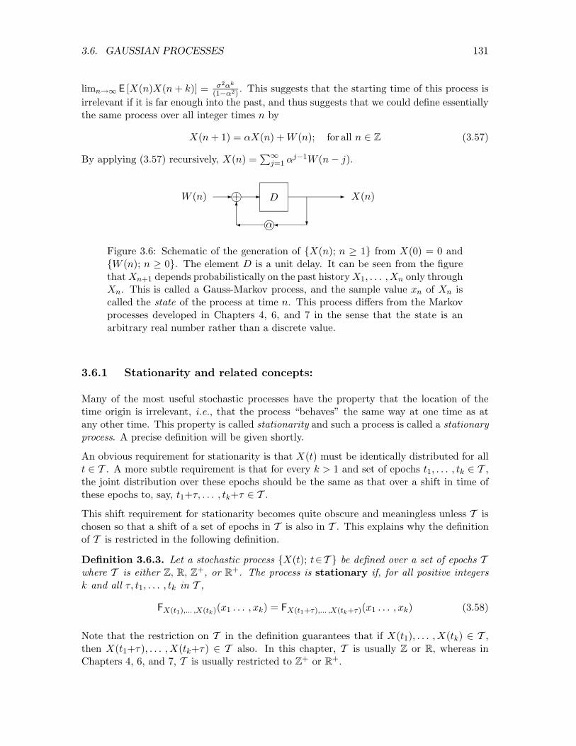
(1�↵2) . This suggests that the starting time of this process isirrelevant if it is far enough into the past, and thus suggests that we could define essentiallythe same process over all integer times n by
X(n + 1) = ↵X(n) + W (n); for all n 2 Z (3.57)
By applying (3.57) recursively, X(n) =P1
j=1 ↵j�1W (n� j).
W (n) - i - D - X(n)
?�i�
6
↵
Figure 3.6: Schematic of the generation of {X(n); n � 1} from X(0) = 0 and{W (n); n � 0}. The element D is a unit delay. It can be seen from the figurethat Xn+1 depends probabilistically on the past history X1, . . . ,Xn only throughXn. This is called a Gauss-Markov process, and the sample value xn of Xn iscalled the state of the process at time n. This process di↵ers from the Markovprocesses developed in Chapters 4, 6, and 7 in the sense that the state is anarbitrary real number rather than a discrete value.
3.6.1 Stationarity and related concepts:
Many of the most useful stochastic processes have the property that the location of thetime origin is irrelevant, i.e., that the process “behaves” the same way at one time as atany other time. This property is called stationarity and such a process is called a stationaryprocess. A precise definition will be given shortly.
An obvious requirement for stationarity is that X(t) must be identically distributed for allt 2 T . A more subtle requirement is that for every k > 1 and set of epochs t1, . . . , tk 2 T ,the joint distribution over these epochs should be the same as that over a shift in time ofthese epochs to, say, t1+⌧, . . . , tk+⌧ 2 T .
This shift requirement for stationarity becomes quite obscure and meaningless unless T ischosen so that a shift of a set of epochs in T is also in T . This explains why the definitionof T is restricted in the following definition.
Definition 3.6.3. Let a stochastic process {X(t); t2T } be defined over a set of epochs Twhere T is either Z, R, Z+, or R+. The process is stationary if, for all positive integersk and all ⌧, t1, . . . , tk in T ,
FX(t1),... ,X(tk)(x1 . . . , xk) = FX(t1+⌧),... ,X(tk+⌧)(x1 . . . , xk) (3.58)
Note that the restriction on T in the definition guarantees that if X(t1), . . . ,X(tk) 2 T ,then X(t1+⌧), . . . ,X(tk+⌧) 2 T also. In this chapter, T is usually Z or R, whereas inChapters 4, 6, and 7, T is usually restricted to Z+ or R+.

132 CHAPTER 3. GAUSSIAN RANDOM VECTORS AND PROCESSES
The discrete-time IID Gaussian process in Example 3.6.1 is stationary since all joint dis-tributions of a given number of distinct variables from {W (n); n 2 Z} are the same. Moregenerally, for any Gaussian process, the joint distribution of X(t1), . . . ,X(tk) depends onlyon the mean and covariance of those variables. In order for this distribution to be the sameas that of X(t1 + ⌧), . . . ,X(tk + ⌧), it is necessary that E [X(t)] = E [X(0)] for all epochs tand also that KX(t1, t2) = KX(t1+⌧, t2+⌧) for all epochs t1, t2, and ⌧ . This latter condi-tion can be simplified to the statement that KX(t, t+u) is a function only of u and not oft. It can be seen that these conditions are also su�cient for a Gaussian process {X(t)} tobe stationary. We summarize this in the following theorem.
Theorem 3.6.2. A Gaussian process {X(t); t2T } (where T is Z, R, Z+, or R+) is sta-tionary if and only if E [X(t)] = E [X(0)] and KX(t, t+u) = KX(0, u) for all t, u 2 T .
With this theorem, we see that the Gauss Markov process of Example 3.6.3, extended tothe set of all integers, is a discrete-time stationary process. The Gaussian sum process ofExample 3.6.2, however, is non-stationary.
For non-Gaussian processes, it is frequently di�cult to calculate joint distributions in orderto determine if the process is stationary. There are a number of results that depend only onthe mean and the covariance function, and these make it convenient to have the followingmore relaxed definition:
Definition 3.6.4. A stochastic process {X(t); t 2 T } (where T is Z, R, Z+, or R+) iswide sense stationary7 (WSS) if E [X(t)] = E [X(0)] and KX(t, t+u) = KX(0, u) forall t, u 2 T .
Since the covariance function KX(t, t+u) of a stationary or WSS process is a function ofonly one variable u, we will often write the covariance function of a WSS process as afunction of one variable, namely KX(u) in place of KX(t, t+u). The single variable inthe single-argument form represents the di↵erence between the two arguments in the two-argument form. Thus, the covariance function KX(t, ⌧) of a WSS process must be a functiononly of t � ⌧ and is expressed in single-argument form as KX(t � ⌧). Note also that sinceKX(t, ⌧) = KX(⌧, t), the covariance function of a WSS process must be symmetric, i.e.,KX(u) = KX(�u),
The reader should not conclude from the frequent use of the term WSS in the literaturethat there are many important processes that are WSS but not stationary. Rather, the useof WSS in a result is used primarily to indicate that the result depends only on the meanand covariance.
3.6.2 Orthonormal expansions
The previous Gaussian process examples were discrete-time processes. The simplest way togenerate a broad class of continuous-time Gaussian processes is to start with a discrete-timeprocess (i.e., a sequence of jointly-Gaussian rv’s) and use these rv’s as the coe�cients in
7This is also called weakly stationary, covariance stationary, and second-order stationary.

3.6. GAUSSIAN PROCESSES 133
an orthonormal expansion. We describe some of the properties of orthonormal expansionsin this section and then describe how to use these expansions to generate continuous-timeGaussian processes in Section 3.6.3.
A set of functions {�n(t); n � 1} is defined to be orthonormal ifZ 1
�1�n(t)�⇤k(t) dt = �nk for all integers n, k. (3.59)
These functions can be either complex or real functions of the real variable t; the complexcase (using the reals as a special case) is most convenient.
The most familiar orthonormal set is that used in the Fourier series.
�n(t) =
8<:
(1/p
T ) exp[i2⇡nt/T ] for |t| T/2
0 for |t| > T/2. (3.60)
We can then take any square-integrable real or complex function x(t) over (�T/2, T/2) andessentially8 represent it by
x(t) =Xn
xn�n(t) ; where xn =Z T/2
�T/2x(t)�⇤n(t)dt (3.61)
The complex exponential form of the Fourier series could be replaced by the sine/cosineform when expanding real functions (as here). This has the conceptual advantage of keepingeverying real, but doesn’t warrant the added analytical complexity.
Many features of the Fourier transform are due not to the special nature of sinusoids,but rather to the fact that the function is being represented as a series of orthonormalfunctions. To see this, let {�n(t); n 2 Z} be any set of orthonormal functions, and assumethat a function x(t) can be represented as
x(t) =Xn
xn�n(t). (3.62)
Multiplying both sides of (3.62) by �⇤m(t) and integrating,Z
x(t)�⇤m(t)dt =Z X
n
xn�n(t)�⇤m(t)dt.
Using (3.59) to see that only one term on the right is non-zero, we getZ
x(t)�⇤m(t)dt = xm. (3.63)
8More precisely, the di↵erence between x(t) and its Fourier seriesP
n xn�n(t) has zero energy, i.e.,R ��x(t) �P
n xn�n(t)��2 dt = 0. This allows x(t) and
Pn xn�n(t) to di↵er at isolated values of t such
as points of discontinuity in x(t). Engineers view this as essential equality and mathematicians define itcarefully and call it L2 equivalence.

134 CHAPTER 3. GAUSSIAN RANDOM VECTORS AND PROCESSES
We don’t have the mathematical tools to easily justify this interchange and it would takeus too far afield to acquire those tools. Thus for the remainder of this section, we willconcentrate on the results and ignore a number of mathematical fine points.
If a function can be represented by orthonormal functions as in (3.62), then the coe�cients{xn} must be determined as in (3.63), which is the same pair of relations as in (3.61).We can also represent the energy in x(t) in terms of the coe�cients {xn; n 2 Z}. Since|x2(t)| = (
Pn xn�n(t))(
Pm x⇤m�⇤m(t)), we getZ
|x2(t)|dt =Z X
n
Xm
xnx⇤m�n(t)�⇤m(t)dt =Xn
|xn|2. (3.64)
Next suppose x(t) is any square-integrable function and {�n(t); n 2 Z} is an orthonormalset. Let xn =
Rx(t)�⇤n(t)dt. Let ✏k(t) = x(t) �
Pkn=1 xn�n(t) be the error when x(t)
is represented by the first k of these orthonormal functions. First we show that ✏k(t) isorthogonal to �m(t) for 1 m k.
Z✏k(t)�⇤m(t)dt =
Zx(t)�⇤m(t)dt�
Z kXn=1
xn�n(t)�⇤m(t)dt = xm � xm = 0. (3.65)
Viewing functions as vectors, ✏k(t) is the di↵erence between x(t) and its projection on thelinear subspace spanned by {�n(t); 1 n k}. The integral of the magnitude squarederror is given by
Z|x2(t)|dt =
Z �����✏k(t) +kX
n=1
xn�n(t)
�����2
dt (3.66)
=Z
|✏2k(t)|dt +Z kX
n=1
kXn=1
xnx⇤m�n(t)�⇤m(t)dt (3.67)
=Z
|✏2k(t)|dt +kX
n=1
|x2n|. (3.68)
Since |✏2k(t)|dt � 0, the following inequality, known as Bessel’s inequality, follows.
kXn=1
|x2n|
Z|x2(t)|dt. (3.69)
We see from (3.68) thatR|✏2k(t)|2dt is non-increasing with k. Thus, in the limit k ! 1,
either the energy in ✏k(t) approaches 0 or it approaches some positive constant. A set oforthonormal functions is said to span a class C of functions if this error energy approaches0 for all x(t) 2 C. For example, the Fourier series set of functions in (3.60) spans the set offunctions that are square integrable and zero outside of [�T/2, T/2]. There are many othercountable sets of functions that span this class of functions and many others that span theclass of square-integrable functions over (�1,1).
In the next subsection, we use a sequence of independent Gaussian rv’s as coe�cients in theseorthonormal expansions to generate a broad class of continuous-time Gaussian processes.

3.6. GAUSSIAN PROCESSES 135
3.6.3 Continuous-time Gaussian processes
Given an orthonormal set of real-valued functions, {�n(t); n 2 Z} and given a sequence{Xn; n 2 Z} of independent rv’s9 with Xn ⇠ N (0,�2
n), consider the following expression:
X(t) = lim`!1
X̀n=�`
Xn�n(t). (3.70)
Note that for any given t and `, the sum above is a Gaussian rv of varianceP`
n=�` �2n�2
n(t).If this variance increases without bound as ` ! 1, then it is not hard to convince oneselfthat there cannot be a limiting distribution, so there is no limiting rv. The more importantcase of bounded variance is covered in the following theorem. Note that the theorem doesnot require the functions �n(t) to be orthonormal.
Theorem 3.6.3. Let {Xn; n 2 Z} be a sequence of independent rv’s, Xn ⇠ N (0,�2n) and
let {�n(t); n 2 Z} be a sequence of real-valued functions. Assume thatP`
n=�` �2n�2
n(t)converges to a finite value as ` ! 1 for each t. Then {X(t); t 2 R} as given in (3.70) isa Gaussian process.
Proof: The di�cult part of the proof is showing that X(t) is a rv for any given t un-der the conditions of the theorem. This means that, for a given t, the sequence of rv’s{P`
n=�` Xn�n(t); ` � 1} must converge WP1 to a rv as ` !1. This is proven in Section9.9.2 as a special case of the martingale convergence theorem, so we simply accept thatresult for now. Since this sequence converges WP1, it also converges in distribution, so,since each term in the sequence is Gaussian, the limit is also Gaussian. Thus X(t) existsand is Gaussian for each t.
Next, we must show that for any k, any t1, . . . , tk, and any a1, . . . , ak, the sum a1X(t1) +· · · + akX(tk) is Gaussian. This sum, however, is just the limit
lim`!1
X̀n=�`
[a1Xn�n(t1) + · · · + akXn�n(tk)].
This limit exists and is Gaussian by the same argument as used above for k = 1. Thus theprocess is Gaussian.
Example 3.6.4. First consider an almost trivial example. Let {�n(t); n 2 Z} be a se-quence of unit pulses each of unit duration, i.e., �n(t) = 1 for n t < n + 1 and �n(t) = 0elsewhere. Then X(t) = Xbtc. In other words, we have converted the discrete-time process{Xn; n 2 Z} into a continuous time process simply by maintaining the value of Xn as aconstant over each unit interval.
Note that {Xn; n 2 Z} is stationary as a discrete-time process, but the resulting continuous-time process is non-stationary because the covariance of two points within a unit intervaldi↵ers from that between the two points shifted so that an integer lies between them.
9Previous sections have considered possibly complex orthonormal functions, but we restrict them here tobe real. Using rv’s (which are real by definition) with complex orthonormal functions is an almost trivialextension, but using complex rv’s and complex functions is less trivial and is treated in Section 3.7.8.

136 CHAPTER 3. GAUSSIAN RANDOM VECTORS AND PROCESSES
Example 3.6.5 (The Fourier series expansion). Consider the real-valued orthonormalfunctions in the sine/cosine form of the Fourier series over an interval [�T/2, T/2), i.e.,
�n(t) =
8>>>>>><>>>>>>:
p2/T cos(2⇡nt/T ) for n > 0, |t| T/2p
1/T for n = 0, |t| T/2p2/T sin(�2⇡nt/T ) for n < 0, |t| T/2
0 for |t| > T/2
.
If we represent a real-valued function x(t) over (�T/2, T/2) as x(t) =P
n xn�n(t), then thecoe�cients xn and x�n essentially represent how much of the frequency n/T is contained inx(t). If an orchestra plays a particular chord during (�T/2, T/2), then the correspondingcoe�cients of Xn will tend to be larger in magnitude than the coe�cients of frequenciesnot in the chord. If there is considerable randomness in what the orchestra is playing thenthese coe�cients might be modeled as rv’s.
When we represent a zero-mean Gaussian process, X(t) =P
n Xn�n(t), by these orthonor-mal functions, then the variances �2
n signify, in some sense that will be refined later, how theprocess is distributed between di↵erent frequencies. We assume for this example that thevariances �2
n of the Xn satisfyP
n �2n < 1, since this is required to ensure that E
⇥X2(t)
⇤is finite for each t. The only intention of this example is to show, first, that a Gaussianprocess can be defined in this way, second that joint probability densities over any finiteset of epochs, �T/2 < t1 < t2 < · · · < tn < T/2 are in principle determined by {�2
n; n2Z},and third, that these variances have some sort of relation to the frequency content of theGaussian process.
The above example is very nice if we want to model noise over some finite time interval.As suggested in Section 3.6.1, however, we often want to model noise as being stationaryover (�1, 1). Neither the interval (�T/2, T/2) nor its limit as T ! 1 turn out to bevery productive in this case. The next example, based on the sampling theorem of linearsystems, turns out to work much better.
3.6.4 Gaussian sinc processes
The sinc function is defined to be sinc(t) = sin(⇡t)⇡t and is sketched in Figure 3.7.
The Fourier transform of sinc(t) is a square pulse that is 1 for |f | 1/2 and 0 elsewhere.This can be verified easily by taking the inverse transform of the square pulse. The mostremarkable (and useful) feature of the sinc function is that it and its translates over integerintervals form an orthonormal set, i.e.,
Zsinc(t� n)sinc(t� k) dt = �nk for n, k 2 Z. (3.71)
This can be verified (with e↵ort) by direct integration, but the following approach is moreinsightful: the Fourier transform of sinc(t � n) is e�i2⇡nf for |f | 1/2 and is 0 elsewhere.

3.6. GAUSSIAN PROCESSES 137
0 1 2 3�1�2
sinc(t) = sin(⇡t)/⇡t
1
Figure 3.7: The function sinc(t) is 1 at t = 0 and 0 at every other integer t. Theamplitude of its oscillations goes to 0 with increasing |t| as 1/|t|
Thus the Fourier transform of sinc(t�n) is easily seen to be orthonormal to that of sinc(t�k)for n 6= k. By Parseval’s theorem, then, sinc(t�n) and sinc(t�k) are themselves orthonormalfor n 6= k.
If we now think of representing any square-integrable function of frequency, say v(f) overthe frequency interval (�1/2, 1/2) by a Fourier series, we see that v(f) =
Pn vnei2⇡nf over
f 2 (�1/2, 1/2), where vn =R 1/2�1/2 v(f)e�i2⇡nf df . Taking the inverse Fourier transform we
see that any function of time that is frequency limited to (�1/2, 1/2) can be representedby the set {sinc(t � n); n 2 Z}. In other words, if x(t) is a square-integrable continuous10function whose Fourier transform is limited to f 2 [�1/2, 1/2], then
x(t) =Xn
xnsinc(t� n) where xn =Z
x(t)sinc(t� n) dt (3.72)
There is one further simplification that occurs here: for any integer value of t, say t = k,sinc(t�n) = �kn, so x(n) = xn. Thus for any square-integrable continuous function, limitedin frequency to [�1/2, 1/2],
x(t) =Xn
x(n)sinc(t� n) (3.73)
This sinc function expansion (better known as the sampling theorem expansion) is muchmore useful when it is linearly scaled in time, replacing the functions sinc(t � n) withsinc(2Bt � n) for some given bandwidth B > 0 (see Figure 3.8). The set of functions{sinc(2Bt � n); n 2 Z} is still an orthogonal set, but the scaling in time by a factor of(2B)�1 causes the squared integral to become (2B)�1. Since the scaling by (2B)�1 in timecauses a scaling of 2B in frequency, these orthogonal function are now limited in frequencyto [�B,B]. The argument above, applied to this scaled orthogonal set, leads to the wellknown sampling theorem:
10The reason for requiring continuity here is that a function can be altered at a finite (or even countable)number of points without changing its Fourier transform. The inverse transform of the Fourier transform ofa bandlimited function, however, is continuous and is the function referred to. It is the same as the originalfunction except at those originally altered points. The reader who wants a more complete development hereis referred to [10].

138 CHAPTER 3. GAUSSIAN RANDOM VECTORS AND PROCESSES
01
2B2
2B�12B
�22B
sinc(2Bt) sinc(2Bt� 1)
1
Figure 3.8: The function sinc(2Bt) is 1 at t = 0 and 0 at every other integermultiple of (2B)�1. The function sinc(2Bt�1) is 1 at t = (2B)�1 and 0 at everyother integer multiple of (2B)�1
Theorem 3.6.4. Let x(t) be a continuous square-integrable real or complex function oft 2 R which is limited in frequency to [�B,B] for any given B > 0. Then
x(t) =Xn
x⇣ n
2B
⌘sinc(2Bt� n) (3.74)
This theorem adds precision to the notion that any well-behaved function of a real variablecan be approximated by its samples, saying that if the function is frequency limited, thensu�ciently close samples represent the function perfectly when the points between thesamples are filled in by this sinc expansion.
Now suppose that {Xn; n 2 Z} is a sequence of IID Gaussian rv’s and consider the followingGaussian sinc process,
X(t) =1X�1
Xnsinc(2Bt� n); where Xn ⇠ N (0,�2) (3.75)
The following theorem shows that the Gaussian sinc process of (3.75) is indeed a Gaussianprocess, calculates its covariance function, and shows that the process is stationary.
Theorem 3.6.5. The Gaussian sinc process {X(t); t 2 R} in (3.75) is a stationary Gaus-sian process with
KX(t) = �2sinc(2Bt). (3.76)
Proof: From (3.75), we have
KX(t, ⌧) = E
" Xn
Xnsinc(2Bt� n)
! Xk
Xksinc(2B⌧ � k)
!#
= E
"Xn
X2n sinc(2Bt� n)sinc(2B⌧ � n)
#(3.77)
= �2Xn
sinc(2Bt� n)sinc(2B⌧ � n) (3.78)
= �2sinc(2B(t� ⌧)), (3.79)

3.6. GAUSSIAN PROCESSES 139
where (3.77) results from E [XnXk] = 0 for k 6= n and (3.78) results from E⇥X2
n
⇤= �2 for
all n. To establish the identity between (3.78) and (3.79), let y(t) = sinc(2B(t� ⌧)) for anygiven ⌧ . The Fourier transform of y(t) is Y (f) =
p(2B)�1 exp(�i2⇡B⌧f) for �B f B
and 0 elsewhere. Thus y(t) is frequency limited to [�B,B] and therefore satisfies (3.74),which is the desired identity.
Now note that KX(t, t) = �2 = �2Pn sinc2(2Bt � n). Thus this series converges, and
from Theorem 3.6.3, {X(t); t 2 R} is a Gaussian process. Finally, since the covariancedepends only on t� ⌧ , the process is stationary and the covariance in single variable formis KX(t) = �2sinc(2Bt).
3.6.5 Filtered Gaussian sinc processes
Many important applications of stochastic processes involve linear filters where the filterinput is one stochastic process and the output is another. The filter might be some physicalphenomenon, or it might be a filter being used to detect or estimate something from theinput stochastic process. It might also be used simply to demonstrate the existence ofa stochastic process with certain properties. In this section, we restrict our attention tothe case where the input stochastic process is the Gaussian sinc process described in theprevious section. We then show that the output is a stationary Gaussian process and findits covariance function. Figure 3.9 illustrates the situation.
{X(t); t2R} - h(t) - {Y (t); t2R}
Figure 3.9: A stochastic process {X(t); t 2 R} is the input to a linear time-invariant filter, and the output is another stochastic process. A WSS inputleads to a WSS output and a Gaussian input leads to a Gaussian output.
A linear time-invariant filter with impulse response h(t) creates a linear transformation froman input function x(t) to an output function y(t) defined by y(t) =
R1�1 x(⌧)h(t� ⌧) d⌧ . In
other words, the output at time t is a linear combination of the inputs over all time. Thetime invariance refers to the property that if the input function is translated by a given d,then the output function is translated by the same d.
In many situations, h(t) is restricted to be realizable, meaning that h(t) = 0 for t < 0. Thisindicates that the output at a given t is a function only of the inputs up to and includingt. In other situations, the filtering is done ‘o↵-line,’ meaning that the entire function x(t)is available before performing the filtering. In some cases, the time reference at the filteroutput might have a delay of d relative to that at the input. This often occurs when acommunication channel is subject to both filtering and propagation delay, and in thesecases, h(t) might be non-zero for all t � �d; this can still be regarded as a realizable filter,since only the time reference at the output has been altered.
In this section, we assume that h(t) has a Fourier transform that is 0 for |f | > B, where B

140 CHAPTER 3. GAUSSIAN RANDOM VECTORS AND PROCESSES
is the bandwidth of the input Gaussian sinc process. We shall find later that this impliesthat the filter is non-realizable. This is of no concern here since our purpose is simply tocharacterize a family of Gaussian processes at the filter output.
Suppose a stochastic process {X(t); t 2 R} is the input to a linear time-invariant (LTI)filter. Let ⌦ be the underlying sample space and let ! be a sample point of ⌦. Thecorresponding sample function of the process {X(t); t2R} is then X(t,!). The output ofthe LTI filter with impulse response h(t) and input X(t,!) is given by
Y (t,!) =Z 1
�1X(⌧,!)h(t� ⌧)d⌧.
If the integrals exist for each !, this (in principle) defines a rv for each t and thus (inprinciple) defines a stochastic process {Y (t); t 2 R}. Developing a theory of integration fora continuum of rv’s is quite di�cult11 and would take us too far afield. This is why we areconcentrating on stochastic processes that can be represented as orthonormal expansionsusing a sequence of rv’s as coe�cients. The next section generalizes this to other inputprocesses that can also be represented as orthogonal expansions.
If we express the input sinc process X(t) as in (3.75), then the output process is given by
Y (t) =Z 1
�1
Xn
Xnsinc(2B⌧ � n)h(t� ⌧) d⌧ where Xn ⇠ N (0,�2). (3.80)
Assuming that the integration and summation can be interchanged, we see thatZ 1
�1sinc(2B⌧ � n)h(t� ⌧) d⌧ =
Z 1
�1sinc(2B⌧)h(t� n
2B� ⌧) d⌧
=1
2Bh⇣t� n
2B
⌘, (3.81)
where we have viewed the convolution as a product in the frequency domain and used thefact that the transform of the sinc function is constant over [�B,B] and that H(f) is zerooutside that range. Thus, substituting (3.81) into (3.80) we have
Y (t) =Xn
Xn
2Bh⇣t� n
2B
⌘. (3.82)
From Theorem 3.6.3, ifP
n h2(t�n/2B) is finite for each t, then {Y (t); t 2 R} is a Gaussianprocess (and the previous interchange of integration and summation is justified). Exercise3.22 shows that
Pn h2(t � n/2B) =
R1�1 h2(⌧) d⌧ for each t. This shows that if h(t) is
square integrable, then Y (t) is a Gaussian process.
In the next section, we show that when a WSS stochastic process is filtered by an LTI filter,the output is also WSS. Thus our final result is that if the Xn are IID and N (0,�2) andif h(t) is square integrable and bandlimited to [�B,B], then Y (t) in (3.82) is a stationaryGaussian process. We discuss this further in the next section.
11Readers who believe that stochastic processes are sort of like ordinary functions and can be integratedand understood in the same way should look at Example 3.6.6.
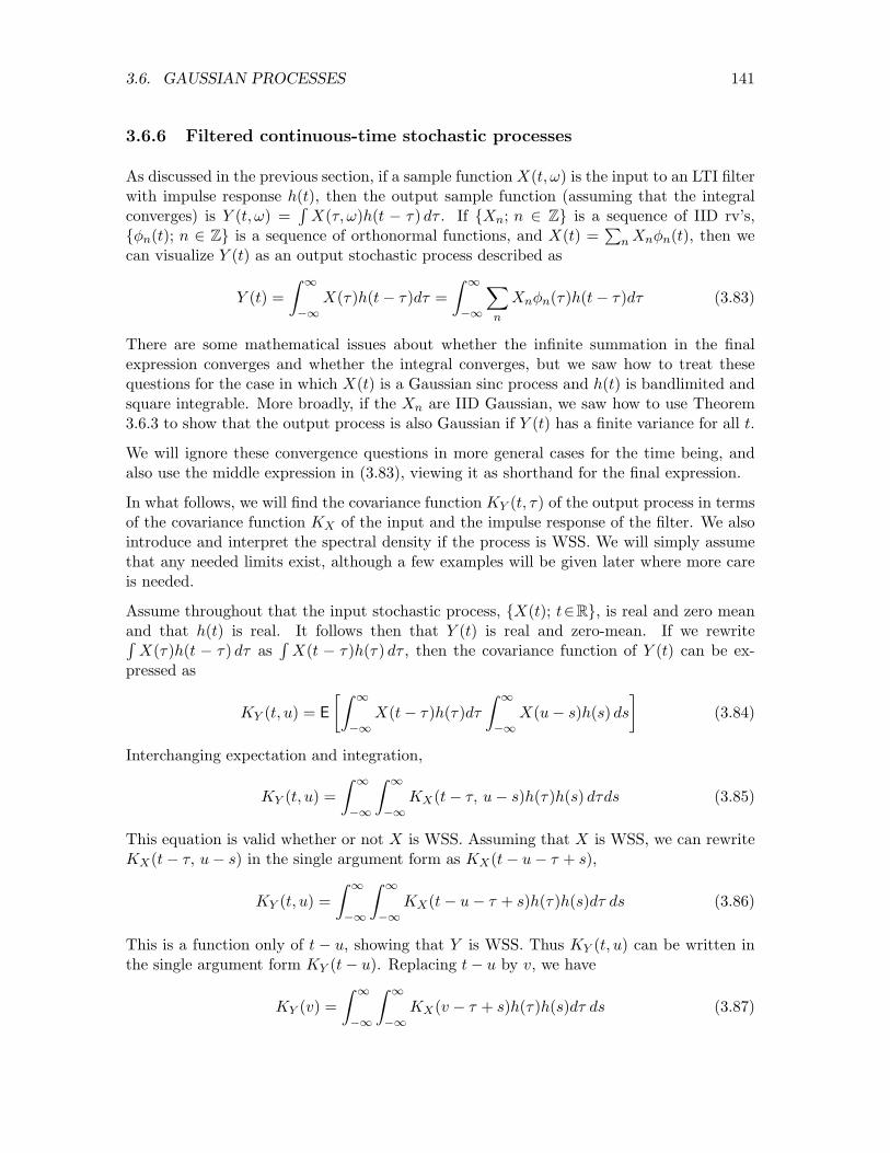
3.6. GAUSSIAN PROCESSES 141
3.6.6 Filtered continuous-time stochastic processes
As discussed in the previous section, if a sample function X(t,!) is the input to an LTI filterwith impulse response h(t), then the output sample function (assuming that the integralconverges) is Y (t,!) =
RX(⌧,!)h(t � ⌧) d⌧ . If {Xn; n 2 Z} is a sequence of IID rv’s,
{�n(t); n 2 Z} is a sequence of orthonormal functions, and X(t) =P
n Xn�n(t), then wecan visualize Y (t) as an output stochastic process described as
Y (t) =Z 1
�1X(⌧)h(t� ⌧)d⌧ =
Z 1
�1
Xn
Xn�n(⌧)h(t� ⌧)d⌧ (3.83)
There are some mathematical issues about whether the infinite summation in the finalexpression converges and whether the integral converges, but we saw how to treat thesequestions for the case in which X(t) is a Gaussian sinc process and h(t) is bandlimited andsquare integrable. More broadly, if the Xn are IID Gaussian, we saw how to use Theorem3.6.3 to show that the output process is also Gaussian if Y (t) has a finite variance for all t.
We will ignore these convergence questions in more general cases for the time being, andalso use the middle expression in (3.83), viewing it as shorthand for the final expression.
In what follows, we will find the covariance function KY (t, ⌧) of the output process in termsof the covariance function KX of the input and the impulse response of the filter. We alsointroduce and interpret the spectral density if the process is WSS. We will simply assumethat any needed limits exist, although a few examples will be given later where more careis needed.
Assume throughout that the input stochastic process, {X(t); t2R}, is real and zero meanand that h(t) is real. It follows then that Y (t) is real and zero-mean. If we rewriteR
X(⌧)h(t � ⌧) d⌧ asR
X(t � ⌧)h(⌧) d⌧ , then the covariance function of Y (t) can be ex-pressed as
KY (t, u) = E
Z 1
�1X(t� ⌧)h(⌧)d⌧
Z 1
�1X(u� s)h(s) ds
�(3.84)
Interchanging expectation and integration,
KY (t, u) =Z 1
�1
Z 1
�1KX(t� ⌧, u� s)h(⌧)h(s) d⌧ds (3.85)
This equation is valid whether or not X is WSS. Assuming that X is WSS, we can rewriteKX(t� ⌧, u� s) in the single argument form as KX(t� u� ⌧ + s),
KY (t, u) =Z 1
�1
Z 1
�1KX(t� u� ⌧ + s)h(⌧)h(s)d⌧ ds (3.86)
This is a function only of t � u, showing that Y is WSS. Thus KY (t, u) can be written inthe single argument form KY (t� u). Replacing t� u by v, we have
KY (v) =Z 1
�1
Z 1
�1KX(v � ⌧ + s)h(⌧)h(s)d⌧ ds (3.87)

142 CHAPTER 3. GAUSSIAN RANDOM VECTORS AND PROCESSES
We now interpret the right hand side of (3.87) as the convolution of three functions. To dothis, we first rewrite (3.87) as
KY (v) =Z
sh(s)
Z⌧KX(v + s� ⌧)h(⌧) d⌧
�ds (3.88)
The term in brackets is the convolution of h and KX evaluated at v + s, which we denoteas [h ⇤KX ](v + s). Now define hb(s) = h(�s). That is, hb is h reversed in time. Replacings with �s, (3.88) becomes
KY (v) =Z
shb(s)[h ⇤KX ](v � s) ds = [hb ⇤ h ⇤KX ](v) (3.89)
One of the simplest and best known results of linear systems is that convolution in the timedomain corresponds to multiplication in the Fourier transform domain. This leads us todefine spectral density.
Definition 3.6.5. The spectral density SY (f) of a WSS stochastic process {Y (t); t 2 R}is the Fourier transform of its covariance function KY (t), i.e.,
SY (f) =Z 1
�1KY (t)e�i2⇡ft dt (3.90)
We now express (3.89) in terms of spectral densities. Let H(f) be the Fourier transform ofthe impulse response h(t),
H(f) =Z 1
�1h(t)e�i2⇡ft dt (3.91)
The Fourier transform of the backward impulse response, hb(t) is then
Hb(f) =Z 1
�1hb(t)e�i2⇡ft dt =
Z 1
�1h(⌧)ei2⇡f⌧ d⌧ = H⇤(f) (3.92)
The transform of (3.89) is then
SY (f) = H⇤(f)H(f)SX(f) = |H(f)|2SX(f) (3.93)
Thus the covariance function of Y (t) is best expressed as the inverse Fourier transform,F�1[|H(f)|2SX(f)].
3.6.7 Interpretation of spectral density and covariance
First note that the covariance function of a real WSS process must be real and symmetricaround 0. Thus SX(f) and SY (f) are real and symmetric around 0. Also, since h(t) is real,|H(f)|2 must be real and symmetric around 0, which is also implied by (3.93).
Now consider a very narrow band filter around some given frequency f0. In particular,assume a filter with frequency response
H(f) =
8<:
1; for f0 � ✏/2 |f | f0 + ✏/2
0; elsewhere.

3.6. GAUSSIAN PROCESSES 143
If we pass a zero-mean WSS stochastic process {X(t)} through this filter, then from (3.93),
SY (f) =
8<:
SX(f); for f0 � ✏/2 |f | f0 + ✏/2
0; elsewhere. (3.94)
The expected power out of this filter, i.e., E⇥Y 2(t)
⇤= KY (0), is independent of t because Y
is WSS. Since KY (t) is the inverse Fourier transform of SY (f), KY (0) = E⇥Y 2(t)
⇤is given
by
E⇥Y 2(t)
⇤=Z
SY (f) df ⇡ 2✏SX(f0). (3.95)
where we assume that SX(f) is continuous and ✏ is so small that SX(f) = SX(�f0) doesnot vary appreciably from f0� ✏/2 to f0 + ✏/2. This means that the expected output powerfrom the filter is proportional to SX(f0). This output power can then be interpreted as theinput power over the range of frequencies ±(f0 � ✏/2, f0 + ✏/2). Since this is proportionalto 2✏ (the aggregate range of positive and negative frequencies in the filter passband), weinterpret spectral density as the power per unit frequency in the WSS process. This alsosays (with a little care about points of discontinuity in SX(f)) that SX(f) � 0 for all f .
Now consider the class of filtered Gaussian sinc processes again. For a Gaussian sinc processbandlimited to B, we have SX(f) = �2/2B for |f | B and SX(f) = 0 for |f | > B. If thisis filtered with frequency response H(f), bandlimited to B, then from (3.93)), we have
SY (f) =
8<:
�2|H(f)|22B for f B,
0 for f > B
There are several remarkable features about this. First, the covariance function KY (t) isdetermined by this spectral density, and since Y (t) is Gaussian, this determines all thejoint distributions of Y (t), i.e., it determines the stochastic process, aside from possibleinteractions with other stochastic processes.
Second, the spectral density, and thus all joint CDF’s depend on H(f) only through |H(f)|2.A given choice for |H(f)|2 can leave significant freedom in choosing H(f), but that freedomdoes not change the joint probability distributions of the process.
Third, since there are essentially no constraints on |H(f)| other than being nonnegative andlimited to B, any desired stationary Gaussian process bandlimited to B can be chosen inthis way. Since B is arbitrary, this limitation does not at first appear significant, althoughthis will be discussed shortly.
Fourth, we have seen that SY (f) � 0 for all f for all WSS stochastic processes. If we restrictour attention to WSS processes for which KY (0) < 1 (and we really can’t make much senseout of other processes), then
RSY (f) df < 1, so it follows that we can approximate SY (f)
by a bandlimited choice with large enough B. Since any bandlimited choice for SY (f) � 0is the spectral density of a filtered Gaussian sinc process, we see that the only constraint onKY (t) to be a covariance function is that KY (0) < 1 and SY (f) � 0 for all f . Furthermore

144 CHAPTER 3. GAUSSIAN RANDOM VECTORS AND PROCESSES
any such spectral density can be approximated (in some sense) by the spectral density of afiltered Gaussian sinc process.
The trouble with filtered Gaussian sinc processes is that realizable filters cannot be bandlim-ited. In fact, the Paley-Wiener theorem (see [19]) says says that a necessary and su�cientcondition on the Fourier transform for a non-zero square-integrable function h(t) to be 0 forall t < 0 is that
R | ln |H(f)k1+f2 df < 1. This is more than an obscure mathematical issue, since
it turns out that bandlimited stationary Gaussian processes have some peculiar propertieseven though their spectral densities closely approximate those of processes that are notbandlimited. We will not resolve these issues here, and readers are urged to exercise carewhen approximating non-bandlimited processes by bandlimited processes.
The purpose of this section has not been to imply that filtered Gaussian sinc processesprovide a universally acceptable way to deal with continuous-time stationary Gaussianprocesses. Rather these banlimited processes provide a great deal of insight into moregeneral stationary Gaussian processes and, with care, can be used to solve a large numberof engineering problems concerning these processes.
3.6.8 White Gaussian noise
Physical noise processes are often well-modeled as stationary Gaussian processes, as wehave pointed out earlier. Often they also have the characteristic that their spectral densityis quite flat over the bandwidths of interest in a given situation. In this latter situation,we can simplify and idealize the model by assuming that the spectral density is constantover all frequencies. This idealization is called white Gaussian noise. Unfortunately, thissimplification comes at a steep price — the power in such a process {W (t); t 2 R} is
E⇥|W (t)|2
⇤= KW (0) =
12⇡
Z 1
�1SW (f)df = 1 (3.96)
Thus W (t) at any given t can not even be approximated as a Gaussian rv. On the otherhand, if a stationary Gaussian process has spectral density SX(f) and is filtered withfrequency function H(f), then, from (3.93) the output process Y (t) has spectral densitySY (f) = |H(f)|2SX(f). If SX(f) is flat over the range of f where H(f) is non-zero, thenthe output Gaussian process {Y (t); t 2 R} has the same joint distributions no matter whatSX(f) is outside the bandwidth of H(f).
If a Gaussian noise process is looked at only through the outputs of various linear filters, andif its spectral density is constant over the frequency response of each filter, then we mightas well assume that the process is white and not concern ourselves with the spectral densityoutside of the range of interest. Since measurement devices generally involve filtering tosome extent (even if flat over such a broad bandwidth that it can usually be ignored), thisview of white Gaussian noise as an idealization is usually the only view that is physicallymeaningful.
In summary then, white Gaussian noise is an idealization of a Gaussian process with spectraldensity12 SW (f) = N0/2 over all f such that |f | B where B is larger than all frequencies
12N0/2 is the standard term among engineers to denote the spectral density of white noise. Spectral

3.6. GAUSSIAN PROCESSES 145
of interest. In the limit B ! 1, the covariance function of white noise can be taken tobe (N0/2)�(t) where �(t) is the Dirac unit impulse. This is a generalized function, roughlydefined by the property that for any well-behaved function a(t), we have
Ra(t)�(t) dt = a(0).
We can visualize �(t) as an idealization of a narrow pulse of unit area, narrow relative tothe smallest interval over which any a(t) of interest can change. With a little thought, Itcan be seen that this is just a another way of saying, as before, that white Gaussian noiseis an idealization of a stationary Gaussian noise process whose spectral density is constantover the frequency range of interest.
One of the nice features of white Gaussian noise is that we can view any zero-mean station-ary Gaussian process as a filtered version of white Gaussian noise. That is, a zero-meanstationary Gaussian process {Y (t); t 2 R} with spectral density SY (f) can be viewed aswhite noise of unit spectral density passed through a filter with frequency response H(f)such that |H(f)|2 = SX(f). Recall that this view was quite valuable in studying Gaussianvectors, and it is equally valuable here.
It almost appears that white Gaussian noise can be viewed as the limit of a sequence ofGaussian sinc processes where process ` has bandwidth B` and power E
⇥X2(t)
⇤= B`N0.
Thus the spectral density for process ` is N0/2 for |f | B`. For any realizable filter withfrequency response H(f), we have observed from the Paley-Wiener theorem that H(f) canonly approach 0 at a limited rate as f ! 1. Thus there is no B large enough that whitenoise filtered by H(f) is quite the same as a filtered sinc Gaussian process, although it couldcertainly be approximated that way.
The following two examples show that we have slightly oversimplified matters in viewingzero-mean stationary Gaussian processes as being characterized by their spectral densities.
Example 3.6.6 (Pathological barely visible Gaussian noise). Consider a stationaryGaussian process {X(t) ; t 2 R} for which X(t) ⇠ N (0, 1) for each t 2 R. Assume thatX(t) and X(⌧) are independent for all t, ⌧ with ⌧ 6= t. Thus KX(t, ⌧) is 1 for t = ⌧ and0 otherwise. This process is Gaussian and stationary, and its single-variable covariancefunction KX(t) is 1 for t = 0 and 0 elsewhere. It follows that SX(f) = 0 for all f . Also, ifwe express X(t) in terms of any set of orthonormal functions, we see that
RX(t)�n(t) dt = 0
WP1 for all n. In the same way, if X(t) is passed through any square-integrable linear filter,the output process is 0 WP1 for all t. Thus in a very real sense, this Gaussian process ise↵ectively 0. From a physical point of view, one could never observe such a process, becauseany physical measurement requires some type of averaging over a very small but non-zerointerval of time. The sample-average measurement over any such interval would then be 0WP1.
We can compare this pathological process to a sequence of Gaussian sinc processes withbandwidths B1 B2, . . . !1 as before. Here, however, we take the power in each processto be 1. Thus the spectral density of the `th process is (2B`)�1 for |f | B`, so the spectraldensity at each f approaches 0 with increasing `. As before, however, there isn’t any decentkind of limit for the process,
density is the power per unit frequency in a process, counting positive and negative frequencies separately.Thus if we look at the power in a bandwidth B, i.e., a frequency interval of width B in positive frequenciesand another B in negative frequencies, the noise power in that band is N0B.

146 CHAPTER 3. GAUSSIAN RANDOM VECTORS AND PROCESSES
There are a number of broad-band communication systems where the transmitted channelwaveform can be roughly modeled as a Gaussian sinc process with large bandwidth andnegligible spectral density. Such a process appears almost non-existant to other commu-nication systems, but as will be seen in Chapter 8 on detection, the signals can still bedetected, in contrast to the strange process here.
The strangeness of the pathological process in this example arises largely from the fact thatthe covariance function is not continuous. Exercise 3.25 shows that if a WSS process hasa covariance function KX(t) that is continuous at t = 0, then it is continuous everywhere.A large part of the theory for constructing orthonormal expansions for continuous randomprocesses depends on a continuous covariance function. From a more application orientedviewpoint, the properties arising from discontinuities in the covariance can not be observed(as in the example here). Thus a continuous covariance function is almost always assumed.
Example 3.6.7 (Pathological invisible Gaussian noise). Let X ⇠ N (0, 1) and let Ybe a uniform rv over (0, 1]. Let Z(t) be a stochastic process where Z(Y ) = X and Z(t) = 0for all t 6= Y . Now for any given t, the probability that Y = t is 0, so Z(t) = 0 WP1. ThusZ(t) can be viewed as Gaussian with variance 0 and, of course, KZ(t) = 0 for all t.
This is more pathological than the previous example, but is important in showing thatspecifying the covariance function of a Gaussian process does not fully specify the process.Here every sample function of this process is discontinuous, whereas the conventional zerofunction is continuous. For any finite set of epochs t1, . . . , tk, we see that X(t1), . . . ,X(tk)are all 0 WP1, so these joint distributions do not distingish this process from the all-zero process. The di↵erence between this process and the all-zero process could never bemeasured, so essentially, the covariance function, and thus the set of finite joint distributions,specify a process. However, as shown here, more intricate tools (common sense for engineersand measure theory for mathematicians) are needed to make sense of continuity for thesesample functions.
3.6.9 The Wiener process / Brownian motion
Recall that one of the major properties of the Poisson counting process (see Chapter 2)is that it has stationary and independent increments. These properties can be be definedfor arbitrary stochastic processes as well as for counting processes. They are fundamentalproperties of the Wiener process, which is also known as Brownian motion.13
Definition 3.6.6. Let a stochastic process {X(t); t2T } be defined over a set of epochs Twhere T is either the nonnegative reals or nonnegative integers. Then {X(t); t 2 T } hasstationary increments if for any epochs t1 < t2, the increment X(t2)�X(t1) has the samedistribution as X(t2 � t1)�X(0).
Definition 3.6.7. Let a stochastic process {X(t); t2T } be defined over a set of epochs Twhere T is either the nonnegative reals or nonnegative integers. Then {X(t); t � 0} has
13Brownian motion is a standard model for the motion of small particles in a gas. Norbert Wienersubstantially developed its mathematical analysis. We will discuss only the one-dimensional version of theprocess.

3.6. GAUSSIAN PROCESSES 147
independent increments if for any sequence of epochs t1 < t2 < t3 < · · · < tk, the randomvariables
[X(t2)�X(t1)], [X(t3)�X(t2)], . . . , [X(tk)�X(tk�1)]
are statistically independent.
Now consider an arbitrary process {X(t); t � 0} with independent and stationary incre-ments and with X(0) = 0. Let � be an arbitrary increment size and, for an arbitrarypositive integer n, write X(n�) as
X(n�) = [X(n�)�X((n� 1)�)] + [X((n� 1)�)�X((n� 2)�)] + · · · + [X(�)�X(0)].
Because of this, we see that E [X(n�)] = nE [X(�)] and VAR [X(n�)] = nVAR [X(�)].Thus the mean and variance of X(t) must each be linear in t. Because of the independentincrements, we can also see that KX(t, ⌧), for any ⌧ � t, is equal to VAR [X(t)]. Wesummarize this in the following theorem.
Theorem 3.6.6. Let {X(t); 0 t} have independent and stationary increments and letX(0) = 0. Then for any epochs t and ⌧ > t,
E [X(t)] = tE [X(1)]] ; KX(t, ⌧) = tVAR [X(1)] (3.97)
One interesting consequence of this is that (except in the uninteresting case of zero vari-ances) processes with independent and stationary increments cannot be stationary. Thatis, {X(t); t � 0} has stationary increments if the changes X(t)�X(t��) do not dependprobabilistically on t, whereas (essentially) the process is stationary if the process valuesthemselves, X(t) do not depend probabilistically on t. Another consequence is that theseprocesses are not meaningful over the entire time interval from �1 to +1. This is becausethe variance is growing linearly with t and must remain nonnegative for all epochs t.
The restriction that X(0) = 0 in the theorem is inessential, and the extension to the casewhere X(0) is an arbitrary rv is contained in Exercise 3.20.
Definition 3.6.8 (The Wiener process / Brownian motion). A Wiener process is azero-mean Gaussian process {X(t); t � 0} which has stationary and independent incre-ments, satisfies X(0) = 0, and has continuous sample functions WP1.
The continuity restriction rules out the addition of ‘invisible’ processes such as that in Ex-ample 3.6.7 to a continuous process with stationary and independent increments. See Feller[14] for a proof that Wiener processes exist. Given this existence, we see that E [X(t)] = 0for all t � 0 and also, from Theorem 3.6.6, KX(t, ⌧) = min(t, ⌧)�2 where �2 = E
⇥X2(1)
⇤.
Since a zero-mean Gaussian process is essentially specified by its covariance function, we seethat the Wiener process is essentially specified by the single parameter �2. Also, since thecovariance function has been derived using only the stationary and incependent incrementsproperty, we see that the added assumption about continuity is not required for specifyingall the joint CDF’s of the process.

148 CHAPTER 3. GAUSSIAN RANDOM VECTORS AND PROCESSES
A type of continuity also follows directly from the independent and stationary incrementproperty without the added requirement of continuity in the definition of a Wiener process.Consider the increment X(t + �)�X(t) for very small �. The increment has the variance��2, and by the Chebyshev inequality,
Pr{X(t + �)�X(t) > ✏} ��2
✏2.
This means that as � ! 0, the probability that X(t) changes by more than ✏ goes to zero.To understand the type of continuity implied by this, consider the sequence X(t+�),X(t+�/2),X(t + �/3), . . . for some given t, �. This sequence approaches X(t) in probability(see Section 1.7.2). This is weaker, of course, than the continuity of sample functions WP1required in the definition of a Wiener process.
Strangely enough, although the sample functions of a Wiener process have these continuityproperties, they are essentially not di↵erentiable. To see this, note that [X(t+�)�X(t)]/�has variance �2/�. This goes to 1 as � ! 0. Despite these strange properties, the Wienerprocess is widely used by engineers, and often provides sound insights into real issues.
The Poisson counting process and Wiener process are similar in the sense that both are, in asense, modeling an “integral” of independent objects. In the Poisson case, we are interestedin random point arrivals. If we view a sample function of these arrivals as a sequence of unitimpulses, then the corresponding sample function of the counting process is the integral ofthat impulse chain. The Wiener process models an accumulation or integral of individuallysmall but very dense independent disturbances (noise). One can envision the process beingintegrated as white Gaussian noise, although, as we have seen, the derivative of the Wienerprocess does not exist and white Gaussian noise does not exist except as a generalized formof stochastic process.
We now show that the Wiener process can be viewed as a limit of a sum of IID rv’s if thelimit uses the appropriate kind of scaling. Let {Yn; n � 1} be a sequence of zero-mean IIDrv’s each with finite variance �2. Consider a sequence of processes {X`(t); t � 0} where the`th process is defined in terms of {Yn; n � 1} by
X`(t) =b2`tcXk=1
2�`/2Yk.
Then E [X`(t)] = 0 and E⇥X2
` (t)⇤
= �2t, where we are ignoring the di↵erence between b2`tcand 2`t.
Note that each unit increase in ` doubles the number of IID rv’s added together in each unitof time. Note also that the magnitude of the IID rv’s are scaled down by the square root ofthis rate doubling. Thus the variance of the scaled sum for a given t remains constant as `increases. By the CLT, the distribution of this scaled sum approaches the Gaussian. It iseasy to see that the covariance of X`(t) approaches that of the Wiener process (in fact, itis only the integer approximation b2`tc ⇡ 2`t that is involved in the covariance).
We don’t want to address the issue of how a limit of a sequence of stochastic processesapproaches another process. The important thing is that a sum of (finite variance zero-

3.7. CIRCULARLY-SYMMETRIC COMPLEX RANDOM VECTORS 149
mean) rv’s can be modeled as a Wiener process with the appropriate scaling; this explainswhy the Wiener process appears in so many applications.
This completes our discussion of (real) Gaussian processes. The next section discusses thecomplex case.
3.7 Circularly-symmetric complex random vectors
Many of the (real-valued) waveforms used for communication and other purposes havethe property that their Fourier transforms are 0 except in two relatively narrow bands offrequencies, one around a positive carrier frequency f0, and the other around �f0. Suchwaveforms are often represented as
x(t) = zre(t) cos(2⇡f0t) + zim(t) sin(2⇡f0t) = <hz(t)e�2⇡if0t
i, i =
p�1.
Representing x(t) in terms of a complex ‘baseband waveform’ z(t) = zre(t) + izim(t) or interms of two real baseband waveforms, zre(t) and zim(t) is often convenient analytically,since if the bandwidth is small and f0 is large, then z(t) changes slowly relative to x(t),while still specifying the waveform exactly for a given f0.
The same relationship, X(t) = <[Z(t) exp[�2⇡if0t], is equally convenient for a stochasticprocess rather than an individual waveform in a limited bandwidth. Note however thatsin(2⇡f0t) is the same as cos(2⇡f0t) except for a small delay, 1/(4f0). Normally, we wouldnot expect the statistics of the noise to be sensitive to this small delay; in more graphicterms, we would not expect the noise to ‘know’ where our time reference t = 0 is. Thus weoften model bandpass noise so that Zre(t) and Zim(t) are identically distributed. By extend-ing this slightly, we often model bandpass noise so that Z(t) and Z(t)e�i✓ are identicallydistributed for all phases ✓. More specifically, we often model bandpass noise so that foreach t1, t2, . . . , tn, the joint distribution of the complex random vector (Z(t1), . . . , Z(tn))T
is the same as that of (Z(t1)ei✓, . . . , Z(tn)ei✓)T for each real ✓.
The purpose of the above argument is not to convince the reader that this joint distributionproperty is ‘necessary’ for band-pass noise, but simply to motivate why this kind of phaseinvariance, which is called circular symmetry, might be useful to understand. The resultshere are widely used in many branches of engineering, mathematics, and physics, but notwidely accessible in a systematic form.
3.7.1 Circular symmetry and complex Gaussian rv’s
Definition 3.7.1. A complex rv Z = Zre + iZim is Gaussian if Zre and Zim are jointlyGaussian; Z is circularly symmetric if Z and Zei✓ have the same distribution for all real ✓.
Note that if Z has a PDF and is circularly symmetric, then the PDF is constant on any circlecentered on the origin. If Z is Gaussian, then its equal probability contours are ellipses;these are circular and centered on the origin if and only if Zre and Zim are IID zero-mean

150 CHAPTER 3. GAUSSIAN RANDOM VECTORS AND PROCESSES
Gaussian. The amplitude |Z| of a circularly-symmetric Gaussian rv is Rayleigh-distributedand the phase is uniformly distributed.
If we multiply a circularly-symmetric rv Z by a complex constant c, then the amplitudeof cZ is the product of the amplitudes of Z and c; the phase is the sum of the individualphases. It is intuitively clear (from the original uniform phase of Z) that such an additionof phases maintains the circular symmetry.
A circularly-symmetric Gaussian rv Z is fully described by its variance, �2 = E [ZZ⇤] =E⇥|Z|2
⇤. The complex conjugate is necessary in the definition of variance, since E [ZZ⇤] =
E⇥Z2
re
⇤+ E
⇥Z2
im
⇤whereas E
⇥Z2
⇤= E
⇥Z2
re
⇤� E
⇥Z2
im
⇤.
Just as a Gaussian rv X of mean a and variance �2 is described as X ⇠ N (a,�2), acircularly-symmetric Gaussian rv Z of variance �2 is described as Z ⇠ CN (0,�2). Notethat the real and imaginary parts of Z are then IID with variance �2/2 each. The termi-nology allows for a complex rv with a mean a and a fluctuation that is circularly-symmetricGaussian to be referred to as CN (a,�2).
Definition 3.7.2. An n-dimensional complex random vector (complex n-rv) Z = (Z1, . . . , Zn)T
is Gaussian if the 2n real and imaginary components of Z are jointly Gaussian. It is circu-larly symmetric if the distribution of Z (i.e., the joint distribution of the real and imaginaryparts) is the same as that of ei✓Z for all phase angles ✓. It is circularly-symmetric Gaussianif it is Gaussian and circularly symmetric.
Example 3.7.1. An important example of a circularly-symmetric Gaussian rv is W =(W1, . . . ,Wn)T where the components Wk, 1 k n are statistically independent and eachis CN (0, 1). Since each Wk, is CN (0, 1), it can be seen that ei✓Wk has the same distributionas Wk. Using the independence, ei✓W then has the same distribution as W . The 2n realand imaginary components of W are IID and N (0, 1/2) so that the probability density(being careful about the factors of 1/2) is
fW (w) =1⇡n
exp
"nX
k=1
�|wk|2#
, (3.98)
where we have used the fact that |wk|2 = <(wk)2 +=(wk)2 for each k to replace a sum over2n terms with a sum over n terms.
3.7.2 Covariance and pseudo-covariance of complex n-rv’s
We saw in Section 3.3.4 that the distribution of a real zero-mean Gaussian n-rv (i.e., a vectorwith jointly-Gaussian components) is completely determined by its covariance matrix. Herewe will find that the distribution of a circularly-symmetric Gaussian n-rv is also determinedby its covariance matrix. Without circular symmetry, the covariance matrix is not su�cientto determine the distribution. In order to understand this, we first define both the covariancematrix and the pseudo-covariance matrix of a complex n-rv.
Definition 3.7.3. The covariance matrix [KZ] and the pseudo-covariance matrix [MZ] ofa zero-mean complex n-rv Z = (Z1, . . . , Zn)T are the n⇥n matrices of complex components

3.7. CIRCULARLY-SYMMETRIC COMPLEX RANDOM VECTORS 151
given respectively by
[KZ] = EhZZ †
i[MZ] = E [ZZT] , (3.99)
where Z † is the the complex-conjugate of the transpose, i.e., Z† = Z T⇤.
As shown below, [KZ ] and [MZ ] determine the covariance matrix of the real 2n-rv
Z re
Z im
�.
E [<(Zk)<(Zj)] =12< ([KZ ]kj + [MZ ]kj) ,
E [=(Zk)=(Zj)] =12< ([KZ ]kj � [MZ ]kj) ,
E [<(Zk)=(Zj)] =12= (�[KZ ]kj + [MZ ]kj) ,
E [=(Zk)<(Zj)] =12= ([KZ ]kj + [MZ ]kj) (3.100)
If Z is also Gaussian, this shows that [KZ ] and [MZ ] together specify not only the covariancebut also the distribution of
Z re
Z im
�, and thus specify the distribution of Z . We next start
to connect the notion of circular symmetry with the pseudo-covariance matrix.
Lemma 3.7.1. Let Z be a circularly-symmetric complex n-rv. Then the pseudo-covariancematrix satisfies [MZ] = 0 .
Proof: Since Z and ei✓Z have the same joint distribution for any given ✓, they havethe same pseudo-covariance matrix, i.e., [Mei✓Z ] = [MZ ]. Denote the j, ` component of[Mei✓Z ] as [Mei✓Z ]j,`. Then
[Mei✓Z ]j,` = Ehei✓Zj · ei✓Z`
i= ei2✓[MZ ]j`.
For i = ⇡/2 then, [MZ ]j,` = �[MZ ]j,`. Thus [MZ ]j,` = 0 for all j, `.
In general, [MZ ] = 0 is not enough to ensure that Z is circularly symmetric. For example,in the one dimensional case, if Zre and Zim are IID, binary equiprobable (1, -1), then[MZ ] = 0 but Z is obviously not circularly symmetric. The next theorem, however, showsthat [MZ ] = 0 is enough in the Gaussian case.
Theorem 3.7.1. Let Z be a zero-mean complex Gaussian n–rv. Then [MZ] = 0 if andonly if Z is circularly-symmetric Gaussian.
Proof: The lemma shows that [MZ ] = 0 if Z is circularly-symmetric. For the only-if side,assume [MZ ] = 0. Then [Mei✓Z ] = 0 also, so [MZ ] = [Mei✓Z ].
We must next consider [Kei✓Z ]. The j, ` component of this matrix for any j, ` is
Ehei✓Zk · e�i✓Z⇤
`
i= E [Zk · Z⇤
` ] = [KZ ]j`.

152 CHAPTER 3. GAUSSIAN RANDOM VECTORS AND PROCESSES
Thus, [Kei✓Z ] = [KZ ], so ei✓Z has the same covariance and pseudo-covariance as Z .
Since ei✓Z and Z are each zero-mean complex Gaussian, each distribution is specified byits covariance and pseudo-covariance. Since these are the same, ei✓Z and Z must have thesame distribution. This holds for all real ✓, so Z is circularly-symmetric Gaussian.
Since [MZ ] is zero for any circularly-symmetric Gaussian n-rv Z , the distribution of Z isdetermined solely by [KZ ] and is denoted as Z ⇠ CN (0, [KZ ]) where C denotes that Z isboth complex and circularly symmetric. The complex normalized IID rv of Example 3.7.1is thus denoted as W ⇠ CN (0, [In]).
The following two examples illustrate some subtleties in Theorem 3.7.1.
Example 3.7.2. Let Z = (Z1, Z2)T where Z1 ⇠ CN (0, 1) and Z2 = XZ1 where X is sta-tistically independent of Z1 and has possible values ±1 with probability 1/2 each. It is easyto see that Z2 ⇠ CN (0, 1), but the real and imaginary parts of Z1 and Z2 together are notjointly Gaussian. In fact, the joint distribution of <(Z1) and <(Z2) is concentrated on thetwo diagonal axes and the distribution of =(Z1) and =(Z2) is similarly concentrated. Thus,Z is not Gaussian. Even though Z1 and Z2 are individually circularly-symmetric Gaussian,Z is not circularly-symmetric Gaussian according to the definition. In this example, it turnsout that Z is circularly symmetric and [MZ ] =
⇥0 00 0
⇤. The example can be changed slightly,
changing the definition of Z2 to <(Z2) = X<(Z1) and =(Z2) ⇠ N (0, 1/2), where =(Z2)is statistically independent of all the other variables. Then [MZ ] is still 0, but Z is notcircularly symmetric. Thus, without the jointly-Gaussian property, the relation betweencircular symmetry and [MZ ] = 0 is not an if-and-only-if relation.
Example 3.7.3. Consider a vector Z = (Z1, Z2)T where Z1 ⇠ CN (0, 1) and Z2 = Z⇤1 . Since
<(Z2) = <(Z1) and =(Z2) = �=(Z1), we see that the four real and imaginary componentsof Z are jointly Gaussian, so Z is complex Gaussian and the theorem applies. We see that[MZ ] =
⇥0 11 0
⇤, and thus Z is Gaussian but not circularly symmetric. This makes sense,
since when Z1 is real (or approximately real), Z2 = Z1 (or Z2 ⇡ Z1) and when Z1 is pureimaginary (or close to pure imaginary), Z2 is the negative of Z1 (or Z2 ⇡ �Z1). Thus therelationship of Z2 to Z1 is certainly not phase invariant.
What makes this example interesting is that both Z1 ⇠ CN (0, 1) and Z2 ⇠ CN (0, 1). Thus,as in Example 3.7.2, it is the relationship between Z1 and Z2 that breaks up the circularly-symmetric Gaussian property. Here it is the circular symmetry that causes the problem,whereas in Example 3.7.2 it was the lack of a jointly-Gaussian distribution.
3.7.3 Covariance matrices of complex n-rv
The covariance matrix of a complex n-rv Z is [KZ ] = E⇥ZZ †⇤. The properties of these
covariance matrices are quite similar to those for real n-rv except that [KZ ] is no longersymmetric (Kkj = Kjk), but rather is Hermitian, defined as a square matrix [K] for whichKkj = K⇤
jk for all j, k. These matrices are analyzed in virtually the same way as thesymmetric matrices considered in Section 3.4.1, so we simply summarize the results weneed here.

3.7. CIRCULARLY-SYMMETRIC COMPLEX RANDOM VECTORS 153
If [K] is Hermitian, then the eigenvalues are all real and the eigenvectors q j and qk ofdistinct eigenvalues are orthogonal in the sense that q†
jqk = 0. Also if an eigenvalue hasmultiplicity `, then ` orthogonal eigenvectors can be chosen for that eigenvalue.
The eigenvalues �1, . . . ,�n, repeating each distinct eigenvalue according to its multiplicity,can be used as the elements of a diagonal matrix [⇤]. To each �j , we can associate aneigenvector q j where the eigenvectors are chosen to be orthonormal (q†
jqk = �jk). Letting[Q] be the matrix with orthonormal columns14 q1, . . . , qn, we have the relationship
[K] = [Q⇤Q�1] [Q†] = [Q�1] for [K] Hermitian. (3.101)
An n⇥ n Hermitian matrix [K] is positive semi-definite if, for all complex n-vectors b, theequation b†[K]b � 0 holds. It is positive definite if b†[K]b > 0 for all b 6= 0. By the sameargments as in the real case, we have the following lemma:
Lemma 3.7.2. If Z is a complex n-rv with covariance matrix [K], then [K] satisfies (3.101)and is positive semi-definite. It is positive definite if [K] is non-singular. Also, for anycomplex n⇥ n matrix [A], the matrix [AA†] is positive semi-definite and is positive definiteif [A] is non-singular. For any positive semi-definite [K], there is a square-root matrix[R] = [Q
p⇤Q�1] as given in (3.101) such that Z = [R]W (where W ⇠ CN (0, I)) is
circularly-symmetric Gaussian with [KZ] = [K].
We have seen that the major change in going from real n-rv’s to complex n-rv’s is a judiciousconversion of transposes into complex-conjugate transposes.
3.7.4 Linear transformations of W ⇠ CN (0, [I`])
One of the best ways to understand real Gaussian n-rv’s is to view them as linear trans-formations of an `-rv (for given `) with IID components, each N (0, 1). The same approachturns out to work equally well for circularly-symmetric Gaussian vectors. Thus let [A] bean arbitrary complex n⇥ ` matrix and let the complex n-rv Z = (Z1, . . . , Zn)T be definedby
Z = [A]W where W ⇠ CN (0, [I`]) (3.102)
The complex n-rv defined by this complex linear transformation has jointly Gaussian realand imaginary parts. To see this, represent the complex n-dimensional transformation in(3.102) by the following 2n dimensional real linear transformation:
Z re
Z im
�=
[Are] �[Aim][Aim] [Are]
� W re
W im
�, (3.103)
where Z re = <(Z ), Z im = =(Z ), [Are] = <([A]), and [A]im = =([A]). By definition, reallinear transformations on real IID Gaussian rv’s have jointly-Gaussian components. ThusZ re and Z im are jointly Gaussian and Z is a complex Gaussian n-rv.
14A square complex matrix with orthonormal columns is said to be unitary. Viewed as a transformation,Qz has the same length as z where the length of z is
pz †z .

154 CHAPTER 3. GAUSSIAN RANDOM VECTORS AND PROCESSES
The rv Z is also circularly symmetric.15 To see this, note that
[KZ ] = Eh[A]WW †[A†]
i= [AA†] [MZ ] = E [[A]WW T[AT]] = 0 (3.104)
Thus, from Theorem 3.7.1, Z is circularly-symmetric Gaussian and Z ⇠ CN (0, [AA†]).
This proves the if part of the following theorem.
Theorem 3.7.2. A complex rv Z is circularly-symmetric Gaussian if and only if it can beexpressed as Z = [A]W for a complex matrix [A] and an IID circularly-symmetric Gaussianrv W ⇠ CN (0, [I]).
Proof: For the only if part, choose [A] to be the square root matrix [R] of Lemma 3.7.2.Then Z = [R]W is circularly-symmetric Gaussian with [KZ ] = [RR†]
We now have three equivalent characterizations for circularly-symmetric Gaussian n-rv’s.First, phase invariance, second, zero pseudo-covariance, and third, linear transformationsof IID circularly symmetric Gaussian vectors. One advantage of the third characterization isthat the jointly-Gaussian requirement is automatically met, whereas the other two dependon that as a separate requirement. Another advantage of the third characterization is thatthe usual motivation for modeling rv’s as circularly-symmetric Gaussian is that they arelinear transformations of essentially IID circularly-symmetric Gaussian random vectors.
3.7.5 Linear transformations of Z ⇠ CN (0, [K])
Let Z ⇠ CN (0, [K]). If some other random vector Y can be expressed as Y = [B]Z ,then Y is also a circularly-symmetric Gaussian random vector. To see this, represent Zas Z = [A]W where W ⇠ CN (0, [I]). Then Y = [BA]W , so Y ⇠ CN (0, [BKB†]). Thishelps show why circular symmetry is important — it is invariant to linear transformations.
If [B] is 1 by n (i.e., if it is a row vector bT) then Y = bTZ is a complex rv. Thus all linearcombinations of a circularly-symmetric Gaussian random vector are circularly-symmetricGaussian rv’s.
Conversely, we now want to show that if all linear combinations of a complex random vectorZ are circularly-symmetric Gaussian, then Z must also be circularly-symmetric Gaussian.The question of being Gaussian can be separated from that of circular symmetry. Thusassume that for all complex n-vectors b, the complex rv bTZ is complex Gaussian. Itfollows that <(bTZ ) = bT
reZ re� bTimZ im is a real Gaussian rv for all choices of bre and b im.
Thus from Theorem 3.4.7, the real 2n-rv
Z re
Z im
�is a Gaussian 2n-rv. By defininition, then,
Z is complex Gaussian.
We could now show that Z is also circularly-symmetric Gaussian if bTZ is circularly-symmetric for all b, but it is just as easy, and yields a slightly stronger result, to show thatif Z is Gaussian and the pairwise linear combinations Zj + Zk are circularly-symmetric forall j, k, then Z ⇠ CN (0, [KZ ]) . If Zj +Zj is circularly symmetric for all j, then E
hZ2
j
i= 0,
15Conversely, as shown later, all circularly-symmetric Gaussian rv’s can be defined this way.

3.7. CIRCULARLY-SYMMETRIC COMPLEX RANDOM VECTORS 155
so that the main diagonal of [MZ ] is zero. If in addition, Zj + Zk is circularly symmetric,then E
⇥(Zj + Zk)2
⇤= 0. But since E
hZ2
j
i= E
⇥Z2
k
⇤= 0, we must have 2E [ZjZk] = 0. Thus
the j, k element of [MZ ] = 0. Thus if Zj + Zk is circularly symmetric for all j, k, it followsthat [MZ ] = 0 and Z is circularly symmetric.16 Summarizing,
Theorem 3.7.3. A complex random vector Z = (Z1, . . . , Zn)T is circularly-symmetricGaussian if and only if all linear combinations of Z are complex Gaussian and Zj + Zk
is circularly symmetric for all j, k.
3.7.6 The PDF of circularly-symmetric Gaussian n-rv’s
Since the probability density of a complex random variable or vector is defined in termsof the real and imaginary parts of that variable or vector, we now pause to discuss theserelationships. The major reason for using complex vector spaces and complex randomvectors is to avoid all the detail of the real and imaginary parts, but our intuition comesfrom R2 and R3, and the major source of confusion in treating complex random vectorscomes from assuming that Cn is roughly the same as Rn. This assumption causes additionalconfusion when dealing with circular symmetry.
Assume that Z ⇠ CN (0, [KZ ]), and let U =
Z re
Z im
�be the corresponding real 2n-rv. Let
[KU ] be the covariance of the real 2n-rv U . From (3.100), with [MZ ] = 0, we can express[KU ] as
[KU ] =
24
12 [Kre] �1
2 [Kim]
12 [Kim] 1
2 [Kre]
35 , (3.105)
where [Kre] is the n⇥ n matrix whose components are the real parts of the components of[KZ ] and correspondingly [Kim] is the matrix of imaginary parts.
Now suppose that (�, q) is an eigenvalue, eigenvector pair for [KZ ]. Separating [KZ ]q = �qinto real and imaginary parts,
[Kre]q re � [Kim]q im = �q re ; [Kim]q re + [Kre]q im = �q im.
Comparing this with [KU ]
qreq im
�, where [KU ] is given in (3.105), we see that �/2 is an
eigenvalue of [KU ] with eigenvector
qreq im
�. Furthermore,assuming that q is normalized
over complex n-space,
qreq im
�is normalized over real 2n-space. As a complex n-vector,
iq (where i =p�1) is a complex scalar times q . It is an eigenvector of [KZ ] but not
independent of q . The corresponding real 2n-vector�q imqre
�, is orthonormal to
qreq im
�and
is also an eigenvector of [KU ]. In addition, for any orthonormal complex n-vectors, thecorresponding real 2n-vectors are orthonormal. This establishes the following lemma.
16Example 3.7.3 showed that if Z is Gaussian with individually circularly symmetric components, thenZ is not necessarily circularly-symmetric Gaussian. This shows that the only additional requirement is forZk + Zj to be circularly-symmetric for all k, j.

156 CHAPTER 3. GAUSSIAN RANDOM VECTORS AND PROCESSES
Lemma 3.7.3. Let (�1, q1), . . . , (�n, qn) denote the n pairs of eigenvalues and orthonormaleigenvectors of the covariance matrix [KZ] of a circularly-symmetric n-rv Z. Then the real2n-rv U =
Zre
Zim
�has a covariance matrix [KU] with the 2n eigenvalue, orthonormal
eigenvector pairs
(�1
2,h
q1,req1,im
i), . . . , (
�n
2,h
qn,reqn,im
i) (
�1
2,h�q1,imq1,re
i), . . . , (
�n
2,h�qn,imqn,re
i). (3.106)
Since the determinant of a matrix is the product of the eigenvalues, we see that
det[KU ] =nY
j=1
✓�j
2
◆2
= 2�2n(det[KZ ])2 (3.107)
Recall that the probability density of Z (if it exists) is the same as the probability density ofU =
Z re
Z im
�, i.e., it is the probability density taken over the real and imaginary components
of Z . This plus (3.107) makes it easy to find the probability density for Z assuming thatZ ⇠ CN (0, [KZ ]).
Theorem 3.7.4. Assume that Z ⇠ CN (0, [KZ]) and assume that [KZ] is non-singular.Then the probability density of Z exists everywhere and is given by
fZ(z) =1
⇡n det[KZ]exp(�z†[K�1
Z ]z). (3.108)
Proof: Since [KZ ] is non-singular, its eigenvalues are all positive, so the eigenvalues of[KU ] are also positive and [KU ] is non-singular. Since Z is circularly-symmetric Gaussian,U =
Z re
Z im
�must be zero-mean Gaussian. Since U is a zero-mean Gaussian 2n-rv, its
PDF is given from (3.22) as
fU (u) =2nY
j=1
1p2⇡µj
exp(�v2j /(2µj), (3.109)
where µj is the jth eigenvalue of [KU ] and vj = aTjuj , where aj is the jth orthonormal
eigenvector of [KU ]. We have seen that the eigenvalues �j of [KZ ] are related to those of[KU ] by µj = �j/2 and µj+n = �j/2 for 1 j n. Similarly the eigenvectors can berelated by aT
j = (qTre,j , q
Tim,j) and aT
j+n = (�qTim,j , q
Tre,j). With a little calculation, we get
v2j + v2
j+n = (qTre,jz re + qT
im,jz im)2 + (�qTim,jz re + qT
re,jz im)2
= [<(q†jz )]2 + [=(q†
jz )]2 = |q†jz |2
Substituting this into (3.109) and recognizing that the density is now given directly in termsof Z ,
fZ (z ) =nY
j=1
1⇡�j
exp(�|q†jz |2/(�j).
=1
⇡n det[KZ ]exp(
nXj=1
�|q†jz |2/(�j). (3.110)

3.7. CIRCULARLY-SYMMETRIC COMPLEX RANDOM VECTORS 157
Finally, recalling that q j is the jth column of [Q],
nXj=1
|q†jz |2/�j = z †[Q⇤�1Q�1]z = z †K�1
Z z .
Substituting this into (3.110) completes the proof.
Note that (3.110) is also a useful expression for the density of circularly-symmetric Gaussiann-rv’s. The geometric picture is not as easy to interpret as for real zero-mean Gaussiann-rv’s, but the regions of equal density are still ellipsoids. In this case, however, ei✓z is onthe same ellipsoid for all phases ✓.
The following theorem summarizes circularly-symmetric Gaussian n-rv.
Theorem 3.7.5. A complex n-rv Z is circularly-symmetric Gaussian if and only if anyone of the following conditions is satisfied.
• Z is a Gaussian n-rv and has the same distribution as ei✓Z for all real �.
• Z is a zero-mean Gaussian n-rv and the pseudo-covariance matrix [MZ] is zero.
• Z can be expressed as Z = [A]W where W ⇠ CN (0, [In]).
• For non-singular [KZ], the probability density of Z is given in (3.108). For singular[KZ], (3.108) gives the density of Z after removal of the deterministically dependentcomponents.
• All linear combinations of Z are complex Gaussian and Zj+Zk is circularly symmetricfor all j, k.
Note that either all or none of these conditions are satisfied. The significance of the theoremis that any one of the conditions may be used to either establish the circularly-symmetricGaussian property or to show that it does not hold. We have also seen (in Lemma 3.7.2)that if K is the covariance matrix for any complex n-rv, then it is also the covariance matrixof some circularly-symmetric Gaussian n-rv.
3.7.7 Conditional PDF’s for circularly symmetric Gaussian rv’s
It turns out that conditional PDF’s for circularly-symmetric Gaussian rv’s are virtuallythe same as those for real-valued rv’s. Operationally, the only di↵erence is that transposesmust be replaced with Hermitian conjugates and the basic form for the unconditional realGaussian PDF must be replaced with the basic form of the unconditional complex circularlysymmetric Gaussian PDF. This is not obvious without going through all the calculationsused to find conditional PDF’s for real rv’s, but the calculations are virtually the same,so we won’t repeat them here. We simply repeat and discuss Theorem 3.5.1, modified asabove.

158 CHAPTER 3. GAUSSIAN RANDOM VECTORS AND PROCESSES
Theorem 3.7.6. Let (X1, . . . ,Xn, Y1, . . . , Ym)T be circularly symmetric and jointly Gaus-sian with the non-singular covariance matrix [K] partitioned into n + m columns and rowsas
[K] =
[KX] [KX·Y][K†
X·Y] [KY]
�[K�1] =
[B] [C][C†] [D]
�
Then the joint PDF of X = (X1, . . . ,Xn)T conditional on Y = (Y1, . . . , Ym)T is given by
fX|Y(x|y) =exp
⇢�⇣x + [B�1C]y
⌘†[B]
⇣x + [B�1C]y
⌘�
(⇡)ndet[B�1], (3.111)
The theorem can be interpreted as saying that X can be represented as X = [G]Y + V ,where Y and V are independent, circularly symmetric, and Gaussian. For a given Y = y ,the conditional density of X can be denoted as CN (�[B�1C]y , [B�1]). The notationCN ([A], [K]) here means that the rv has a mean [A] and a fluctuation around [A] which iscircularly symmetric Gaussian with covariance [B]. Thus, in this case, X , conditional onY = y , is cicularly symmetric with covariance [B]�1 around the mean [B�1C].
The matrix [G] = �[B�1C] and the covariance matrix of V is [B�1]. As in Theorem 3.5.2,the matrices [G] and [KV ] can be expressed directly in terms of the joint covariances of Xand Y as
G = [KX·Y K�1Y ] (3.112)
[KV ] = [KX ]� [KX ·Y K�1Y K†
X ·Y ] (3.113)
Conversely, if X can be expressed as X = GY + V where Y and V are independent andeach circularly-symmetric Gaussian, then it is easy to see that (X T,Y T)T must be circularlysymmetric Gaussian. Using the resultant symmetry between X and Y , we see that theremust be a matrix [H] and a rv Z so that Y = HX +Z where X and Z are independent.We will see how this is used for estimation in Section 10.5
3.7.8 Circularly-symmetric Gaussian processes
In this section, we modify Section 3.6 on continuous-time Gaussian processes to brieflyoutline the properties of circularly-symetric Gaussian processes.
Definition 3.7.4. A circularly-symmetric Gaussian process {X(t); t 2 R} is a complexstochastic process such that for all positive integers k and all choices of epochs t1, . . . , tk 2 R,the complex n-rv with components X(t1), . . . ,X(tk) is a circularly-symmetric Gaussian n-rv.
Now assume that {X(t); t 2 R} is a circularly-symmetric Gaussian process. Since eachn-rv (X(t1), . . . ,X(tk))T is circularly symmetric, the corresponding pseudo-covariance ma-trix is 0 and the covariance matrix specifies the distribution of (X(t1), . . . ,X(tk))T. It

3.7. CIRCULARLY-SYMMETRIC COMPLEX RANDOM VECTORS 159
follows then that the pseudo-covariance function, MX(t, ⌧) = E [X(t)X(⌧)] = 0 for all t, ⌧and the covariance function KX(t, ⌧) = E [X(t)X⇤(⌧)] for all t, ⌧ specifies all finite jointdistributions.
A convenient way of generating a circularly-symmetric Gaussian process is to start with asequence of (complex) orthonormal functions {�n(t); n 2 Z} and a sequence of independentcircularly-symmetric Gaussian rv’s {Xn ⇠ CN (0,�2
n); n 2 Z}. Then ifP
n �2n�2
n(t) < 1for all t, it follows, as in Theorem 3.6.3 for ordinary Gaussian processes, that X(t) =P
n Xn�n(t) is a circularly-symmetric Gaussian process.
One convenient such orthonormal expansion is the set of functions �n(t) = ei2⇡nt/T fort 2 (�T/2, T/2) used in the Fourier series over that time interval. The interpretation hereis very much like that in Example 3.6.5, but here the functions are complex, the rv’s arecircularly symmetric Gaussian, and the arithmetic is over C.
Another particularly convenient such expansion is the sinc-function expansion of Section3.6.4. The sinc functions are real, but the expansion is now over the complex field usingcircularly symmetric rv’s. It is intuitively plausible in this case that the process is circularlysymmetric, since the real and imaginary parts of the process are identically distributed.
A complex stochastic process {X(t); t 2 R} can be filtered by a complex filter with impulseresponse h(t). The output is then the complex convolution Y (⌧) =
RX(t)h(⌧ � t) dt. If
X(t) is a circularly symmetric Gaussian process expressed as an orthonormal expansion,then by looking at Y (⌧) over say ⌧1, . . . , ⌧k, we can argue as before that {Y (⌧); ⌧ 2 R} is acircularly symmetric process if its power is finite at all ⌧ . When circularly symmetric sincprocesses are passed through filters, we have a broad class of circularly symmetric processes.
The definition of stationarity is the same for complex stochastic processes as for (real)stochastic processes, but the CDF over say X(t1), . . . ,X(tk) is now over both the realand imaginary parts of those complex rv’s. If X(t1), . . . ,X(tk) are circularly symmetricGaussian, however, then these distributions are determined by the covariance matrices.Thus, circularly symmetric Gaussian processes are stationary if and only if the covariancefunction satisfies KX(t, t+u)) = KX(0, u).
For a stationary circularly-symmetric Gaussian process {X(t); t 2 R}, the covariance func-tion can be expressed as a function of a single variable, KX(u). This function must beHermition (i.e., it must satisfy KX(t) = K⇤
X(�t)). The Fourier transform of a Hermi-tian function must be real, and by repeating the argument in Section 3.6.7, we see thatthis fourier transform must be nonnegative. This Fourier transform is called the spectraldensity of {X(t); t 2 R}.
The spectral density of a stationary circularly-symmetric Gaussian process has the same in-terpretation as the spectral density of a (real) stationary Gaussian process. White Gaussiannoise is defined and interpreted the same way as in the real case, and can be approximatedin the same way by Gaussian sinc processes.
It is important to understand that these very close analogies between real and complexGaussian processes are actually between real and circularly-symmetric Gaussian processes.A complex Gaussian process that is not circularly symmetric does not have very nice proper-ties and is perhaps better thought of as a pair of processes, one real and one pure imaginary.

160 CHAPTER 3. GAUSSIAN RANDOM VECTORS AND PROCESSES
3.8 Summary
The sum of su�ciently many rv’s that are not too dependent tends toward the Gaussiandistribution, and multiple such sums tend toward a jointly-Gaussian distribution. Therequirements for a set of n rv’s to be jointly Gaussian are far more stringent than therequirement that each be Gaussian alone, but fortunately, as above, the conditions thatlead individual rv’s to be Gaussian often also lead multiple rv’s to be jointly Gaussian.Theorem 3.4.8 collects 4 sets of necessary and su�cient conditions for zero-mean rv’s to bejointly Gaussian. Non-zero-mean rv’s are jointly Gaussian if their fluctuations are jointlyGaussian. Finally, a random vector is defined to be Gaussian if its components are jointlyGaussian.
The distribution of a Gaussian vector Z is completely specified by its mean Z and covariancematrix [KZ ]. The distribution is denoted as N (Z , [KZ ]).
If X1,X2, . . . ,Xn, Y1, . . . , Ym are zero mean and jointly Gaussian with a non-singular co-variance matrix, then the conditional density fX |Y (x | y) is jointly Gaussian for each y .The covariance of this conditional distribution is [KX ]� [KX ·Y K�1
Y KTX ·Y ], which does not
depend on the particular sample value y . The conditional mean, [KX ·Y K�1Y ]y , depends
linearly on y . This situation can be equivalently formulated as X = [G]Y + V , where Vis a zero-mean Gaussian n-rv independent of Y . Using the symmetry between the roles ofX and Y , we have Y = [H]X + Z where X and Z are independent.
A stochastic process {X(t); t 2 T } is a Gaussian process if, for all finite sets t1, . . . , tkof epochs, the rv’s X(t1), . . . ,X(tk) are jointly Gaussian. If T is R or R+, then Gaussianprocesses can be easily generated as orthonormal expansions. When a Gaussian orthonormalexpansion is used as the input to a linear filter, the output is essentially also a Gaussianprocess.
A stochastic process is stationary if all finite joint distributions are invariant to time shifts.It is WSS if the covariance function and mean are invariant to time shifts. A zero-meanGaussian process is stationary if the covariance function is invariant to time shifts, i.e., ifKX(t, t+u) = KX(0, u). Thus a stationary zero-mean Gaussian process is determined byits single-variable covariance function KX(u). A stationary zero-mean Gaussian process isalso essentially determined by its spectral density, which is the Fourier transform of KX(u).
The spectral density SX(f) is interpreted as the process’s power per unit frequency atfrequency f . If a stationary zero-mean Gaussian process has a positive spectral densityequal to a constant value, say N0/2, over all frequencies of interest, it is called whiteGaussian noise. Approximating SX(f) as constant over all f is often convenient, but impliesinfinite aggregate power, which is both mathematically and physically absurd. The Gaussiansinc process also models white Gaussian noise over an arbitrarily broad but finite band offrequencies.
Circularly-symmetric rv’s are complex random variables for which the distribution over thereal and imaginary plane is circularly symmetric. A random vector Z is circularly symmetricif Z and ei✓Z have the same distribution for all phases �. Theorem 3.7.5 collects 5 sets ofnecessary and su�cient conditions for complex random vectors to be circularly-symmetricGaussian.

3.9. EXERCISES 161
Vectors and processes of circularly-symmetric Gaussian rv’s have many analogies with or-dinary Gaussian random vectors and processes, and many of the equations governing thereal case can be converted to the circularly-symmetric case simply by replacing transposesby Hermitian transposes. This is true for conditional distributions also. Unfortunately, thisextreme simplicity relating the equations sometimes hides more fundamental di↵erences.Complex Gaussian random vectors and processes that are not circularly symmetric are usu-ally best modeled as separate real and imaginary parts, since almost all of the insights thatwe might try to transfer from the real to complex case fail except when circular symmetryis present.
3.9 Exercises
Exercise 3.1. a) Let X, Y be IID rv’s, each with density fX(x) = ↵ exp(�x2/2). In part(b), we show that ↵ must be 1/
p2⇡ in order for fX(x) to integrate to 1, but in this part,
we leave ↵ undetermined. Let S = X2 + Y 2. Find the probability density of S in terms of↵.
b) Prove from part (a) that ↵ must be 1/p
2⇡ in order for S, and thus X and Y , to berandom variables. Show that E [X] = 0 and that E
⇥X2
⇤= 1.
c) Find the probability density of R =p
S. R is called a Rayleigh rv.
Exercise 3.2. a) By expanding in a power series in (1/2)r2�2, show that
exp✓
r2�2
2
◆= 1 +
r2�2
2+
r4�4
2(22)+ · · · + r2k�2k
k!2k+ · · · .
b) By expanding erZ in a power series in rZ, show that
gZ(r) = E⇥erZ
⇤= 1 + rE [Z] +
r2E⇥Z2
⇤2
+ · · · +rkE
⇥Zi⇤
(k)!+ · · · .
c) By matching powers of r between parts (a) and (b), show that for all integer k � 1,
EhZ2k
i=
(2k)!�2k
k!2k= (2k � 1)(2k � 3) · · · (3)(1)�2k ; E
hZ2k+1
i= 0.
Exercise 3.3. Let X and Z be IID normalized Gaussian random variables. Let Y =|Z|Sgn(X), where Sgn(X) is 1 if X � 0 and �1 otherwise. Show that X and Y are eachGaussian, but are not jointly Gaussian. Sketch the contours of equal joint probabilitydensity.
Exercise 3.4. a) Let X1 ⇠ N (0,�21) and let X2 ⇠ N (0,�2
2) be independent of X1. Con-volve the density of X1 with that of X2 to show that X1 + X2 is Gaussian, N (0,�2
1 + �22).

162 CHAPTER 3. GAUSSIAN RANDOM VECTORS AND PROCESSES
b) Let W1,W2 be IID normalized Gaussian rv’s . Show that a1W1 + a2W2 is Gaussian,N (0, a2
1+a22. Hint: You could repeat all the equations of part a), but the insightful approach
is to let Xi = aiWi for i = 1, 2 and then use part a) directly.
c) Combine part (b) with induction to show that all linear combinations of IID normalizedGaussian rv’s are Gaussian.
Exercise 3.5. a) Let U be an n-rv with mean m and covariance [K] whose MGF is givenby (3.18). Let X = rTU for an arbitrary real vector r . Show that the MGF of X is givenby gX(r) = exp
⇥rE [X] + r2�2
X/2⇤
and relate E [X] and �2X to m and [K].
b) Show that U is a Gaussian rv.
Exercise 3.6. a) Let Z ⇠ N (0, [K]) be n-dimensional. By expanding in a power series in(1/2)rT[K] r , show that
gZ (r) = exprT[K]r
2
�= 1 +
Pj,k rjrkKj,k
2+ · · · +
⇣Pj,k rjrkKj,k
⌘m
2mm!+ · · · .
b) By expanding erjZj in a power series in rjZj for each j, show that
gZ (r) = E
24exp
0@X
j
rjZj
1A35 =
1Xj1=0
· · ·1X
jn=0
rj11
(j1)!· · · rjn
n
(jn)!EhZj1
1 . . . Zjnn
i.
c) Let D = {j1, j2, . . . , j2m} be a set of 2m distinct integers each between 1 and n. Considerthe term rj1rj2 · · · rj2mE [Zj1Zj2 · · ·Zj2m ] in part (b). By comparing with the set of terms inpart (a) containing the same product rj1rj2 · · · rj2m , show that
E [Zj1Zj2 · · ·Zj2m ] =P
j1j2...j2mKj1j2Kj3j4 · · ·Kj2m�1j2m
2mm!,
where the sum is over all permutations (j1, j2, . . . , j2m) of the set D.
d) Find the number of permutations of D that contain the same set set of unordered pairs({j1, j2}, . . . , {j2m�1, j2m}). For example, ({1, 2}, {3, 4}) is the same set of unordered pairsas ({3, 4}, {2, 1}). Show that
E [Zj1Zj2 · · ·Zjj2m ] =X
j1,j2,... ,j2m
Kj1j2Kj3j4 · · ·Kj2m�1j2m , (3.114)
where the sum is over distinct sets of unordered pairs of the set D. Note: another wayto say the same thing is that the sum is over the set of all permutations of D for whichj2k�1 < j2k for 1 k m and j2k�1 < j2k+1 for 1 ki m� 1.
e) To find EhZj1
1 · · ·Zjnn
i, where j1 + j2 + · · · + jn = 2m, construct the random variables
U1, . . . , U2m, where U1, . . . , Uj1 are all identically equal to Z1, where Uj1+1, . . . , Uj1+j2 areidentically equal to Z2, etc., and use (i) to find E [U1U2 · · ·U2m]. Use this formula to findE⇥Z2
1Z2Z3⇤, E
⇥Z2
1Z22
⇤, and E [Z1]4.

3.9. EXERCISES 163
Exercise 3.7. Let [Q] be an orthonormal matrix. Show that the squared distance betweenany two vectors z and y is equal to the squared distance between [Q]z and [Q]y .
Exercise 3.8. a) Let [K] =⇥ .75
.25.25.75
⇤. Show that 1 and 1/2 are eigenvalues of [K] and
find the normalized eigenvectors. Express [K] as [Q⇤Q�1] where [⇤] is diagonal and [Q] isorthonormal.
b) Let [K 0] = ↵[K] for real ↵ 6= 0. Find the eigenvalues and eigenvectors of [K 0]. Don’t usebrute force—think!
c) Find the eigenvalues and eigenvectors of [Km], where [Km] is the mth power of [K].
Exercise 3.9. Let X and Y be jointly Gaussian with means mX , mY , variances �2X , �2
Y ,and normalized covariance ⇢. Find the conditional density fX|Y (x | y).
Exercise 3.10. a) Let X and Y be zero-mean jointly Gaussian with variances �2X , �2
Y ,and normalized covariance ⇢. Let V = Y 3. Find the conditional density fX|V (x | v). Hint:This requires no computation.
b) Let U = Y 2 and find the conditional density of fX|U (x | u). Hint: first understand whythis is harder than part a).
Exercise 3.11. a) Let (X T,Y T) have a non-singular covariance matrix [K]. Show that[KX ] and [KY ] are positive definite, and thus non-singular.
b) Show that the matrices [B] and [D] in (3.39) are also positive definite and thus non-singular.
Exercise 3.12. Let X and Y be jointly-Gaussian rv’s with means mX and mY , covari-ance matrices [KX ] and [KY ] and cross covariance matrix [KX ·Y ]. Find the conditionalprobability density fX |Y (x | y). Assume that the covariance of (X T,Y T) is non-singular.Hint: think of the fluctuations of X and Y .
Exercise 3.13. a) Let W be a normalized IID Gaussian n-rv and let Y be a Gaussianm-rv. Suppose we would like the joint covariance E [WY T] to be some arbitrary real-valuedn ⇥m matrix [K]. Find the matrix [A] such that Y = [A]W achieves the desired jointcovariance. Note: this shows that any real-valued n ⇥ m matrix is the joint covariancematrix for some choice of random vectors.
b) Let Z be a zero-mean Gaussian n-rv with non-singular covariance [KZ ], and let Y be aGaussian m-rv. Suppose we would like the joint covariance E [ZY T] to be some arbitraryn ⇥ m matrix [K 0]. Find the matrix [B] such that Y = [B]Z achieves the desired jointcovariance. Note: this shows that any real valued n ⇥ m matrix is the joint covariancematrix for some choice of random vectors Z and Y where [KZ ] is given (and non-singular).
c) Now assume that Z has a singular covariance matrix in part b). Explain the constraintsthis places on possible choices for the joint covariance E [ZY T]. Hint: your solution shouldinvolve the eigenvectors of [KZ ].

164 CHAPTER 3. GAUSSIAN RANDOM VECTORS AND PROCESSES
Exercise 3.14. a) Let W = (W1,W2, . . . ,W2n)T be a 2n dimensional IID normalizedGaussian rv. Let S2n = W 2
1 + W 22 + · · · + W 2
2n. Show that S2n is an nth order Erlangrv with parameter 1/2, i.e., that fS2n(s) = 2�nsn�1e�s/2/(n � 1)!. Hint: look at S2 fromExercise 3.1.
b) Let R2n =p
S2n. Find the probability density of R2n.
c) Let v2n(r) be the volume of a 2n dimensional sphere of radius r and let b2n(r) be thesurface area of that sphere, i.e., b2n(r) = dv2n(r)/dr. The point of this exercise is to showhow to calculate these quantities. By considering an infinitesimally thin spherical shell ofthickness � at radius r, show that
fR2n(r) = b2n(r)fW (w) |W :W TW=r2 .
d) Calculate b2n(r) and v2n(r). Note that for any fixed � ⌧ r, the volume within � of thesurface of a sphere of radius r to the total volume of the sphere approaches 1 with increasingn.
Exercise 3.15. a) Solve directly for [B], [C], and [D] in (3.39) for the one dimensionalcase where n = m = 1. Show that (3.40) agrees with (3.37)
Exercise 3.16. a) Express [B], [C], and [D], as defined in (3.39), in terms of [KX ], [KY ]and [KX ·Y ] by multiplying the block expression for [K] by that for [K]�1. You can checkyour solutions against those in (3.46) to (3.48). Hint: You can solve for [B] and [C] bylooking at only two of the four block equations in [KK�1]. You can use the symmetrybetween X and Y to solve for [D].
b) Use your result in part a) for [C] plus the symmetry between X and Y to show that
[BKX ·Y K�1Y ] = [K�1
X KX ·Y D]
c) For the formulations X = [G]Y +V and Y = [H]X +Z where X and Y are zero-mean,jointly Gaussian and have a non-singular combined covariance matrix, show that
[K�1V G] = [HTK�1
Z ] (3.115)
Hint: This is almost trivial from part b), (3.43), (3.44), and the symmetry.
Exercise 3.17. Let X and Z be statistically independent Gaussian rv’s of arbitrary di-mension n and m respectively. Let Y = [H]X + Z where [H] is an arbirary real n ⇥mmatrix.
a) Explain why X1, . . . ,Xn, Z1, . . . , Zm must be jointly Gaussian rv’s. Then explain whyX1, . . . ,Xn, Y1, . . . , Ym must be jointly Gaussian.
b) Show that if [KX ] and [KZ ] are non-singular, then the combined covariance matrix [K]for (X1, . . . ,Xn, Y1, . . . , Ym)T must be non-singular.

3.9. EXERCISES 165
Exercise 3.18. a) Verify (3.56) for k = 0 by the use of induction on (3.54).
b Verify (3.56) for k = 0 directly from (3.55)
c) Verify (3.56) for k > 0 by using induction on k.
d) Verify that
limn!1
E [X(n)X(n + k)] =�2↵k
1� ↵2.
Exercise 3.19. Let {X(t); t2<} be defined by X(t) = tA for all t 2 < where A ⇠ N(0, 1).Show that this is a Gaussian process. Find its mean for each t and find its covariancefunction. Note: The purpose of this exercise is to show that Gaussian processes can be verydegenerate and trivial.
Exercise 3.20. Let {X(t); t � 0} be a stochastic process with independent and stationaryincrements and let X(0) be an arbitrary random variable. Show that E [X(t)] = E [X(0)] +tE [X(1)�X(0)] and that
KX(t, ⌧) = VAR [X(0)] + t [VAR [X(1)]� VAR [X(0)]] .
Exercise 3.21. a) Let X(t) = R cos(2⇡ft + ✓) where R is a Rayleigh rv and the rv ✓ isindependent of R and uniformly distributed over the interval 0 to 2⇡. Show that E [X(t)] =0.
b) Show that E [X(t)X(t + ⌧)] = 12E
⇥R2
⇤cos(2⇡f⌧).
c) Show that X(t); t2< is a Gaussian process.
Exercise 3.22. Let h(t) be a real square-integrable function whose Fourier transform is 0for |f | > B for some B > 0. Show that
Pn h2(2Bt� n) = (1/2B)
Rh2(⌧) d⌧ for all t 2 R.
Hint: find the sampling theorem expansion for a time shifted sinc function.
Exercise 3.23. a) Let Z = (Z1, . . . , Zn)T be a circularly-symmetric n-rv. Show that Zk
is circularly symmetric for each k, 1 k n. Hint: use the definition directly (you cannotassume that Z is also Gaussian).
b) Show that Z1 + Z2 is circularly symmetric. For any complex n-vector c, show that cTZis a circularly symmetric rv.
Exercise 3.24. Let A be a complex Gaussian rv, i.e., A = A1 + iA2 where A1 and A2 arezero-mean jointly-Gaussian real rv’s with variances �2
1 and �22 respectively.
a) Show that E [AA⇤] = �21 + �2
2.
b) Show that
E⇥(AA⇤)2
⇤= 3�4
1 + 3�42 + 2�2
1�22 + 4 (E [A1A2])2 .

166 CHAPTER 3. GAUSSIAN RANDOM VECTORS AND PROCESSES
c) Show that E⇥(AA⇤)2
⇤� 2 (E [AA⇤])2 with equality if and only if A1 and A2 are IID.
Hint: Lower bound (E [A1A2])2 by 0.
d Show that VAR [AA⇤] � (E [AA⇤])2.
Exercise 3.25. Let KX(t) be the covariance function of a WSS process {X(t); t 2 <}.Show that if KX(t) is continuous at t = 0, then it is continuous everywhere. Hint: Youmust show that lim�!0 E [X(0)(X(t + �)�X(t))] = 0 for all t. Use the Schwarz inequality.