1

Gaussian Naïve Bayes, and Logistic Regression

Machine Learning 10-701

Tom M. Mitchell Machine Learning Department

Carnegie Mellon University

January 25, 2010

Required reading: •  Mitchell draft chapter (see course website)

Recommended reading: •  Bishop, Chapter 3.1.3, 3.1.4 •  Ng and Jordan paper (see course website)

Recently: •  Bayes classifiers to learn P(Y|X) •  MLE and MAP estimates for parameters of P •  Conditional independence •  Naïve Bayes make Bayesian learning practical •  Text classification

Today: •  Naïve Bayes and continuous variables Xi:

•  Gaussian Naïve Bayes classifier •  Learn P(Y|X) directly

•  Logistic regression, Regularization, Gradient ascent •  Naïve Bayes or Logistic Regression?

•  Generative vs. Discriminative classifiers

2

Naïve Bayes in a Nutshell Bayes rule:

Assuming conditional independence among Xi’s:

So, classification rule for Xnew = < X1, …, Xn > is:

What if we have continuous Xi ? Eg., image classification: Xi is real-valued ith pixel

3

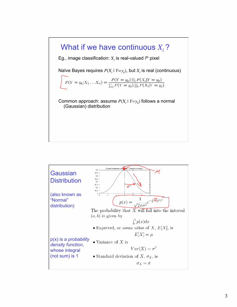
What if we have continuous Xi ? Eg., image classification: Xi is real-valued ith pixel

Naïve Bayes requires P(Xi | Y=yk), but Xi is real (continuous)

Common approach: assume P(Xi | Y=yk) follows a normal (Gaussian) distribution

Gaussian Distribution

(also known as “Normal” distribution)

p(x) is a probability density function, whose integral (not sum) is 1

4

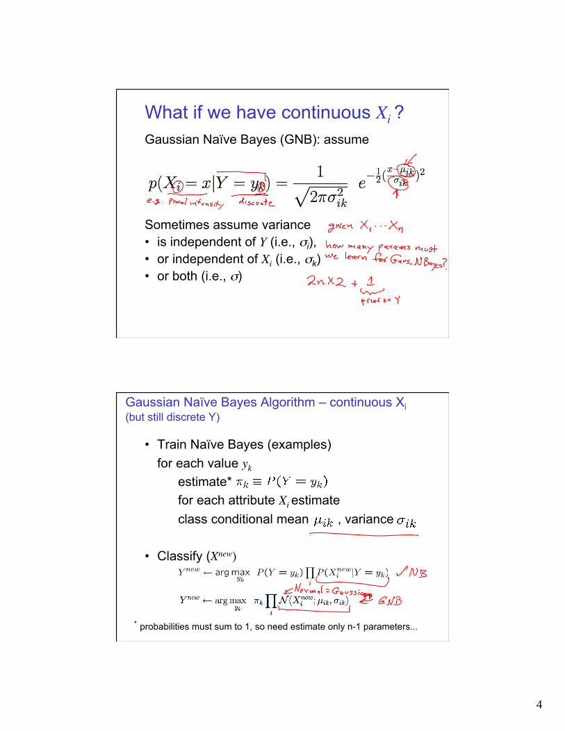
What if we have continuous Xi ? Gaussian Naïve Bayes (GNB): assume

Sometimes assume variance •  is independent of Y (i.e., σi), •  or independent of Xi (i.e., σk) •  or both (i.e., σ)

Gaussian Naïve Bayes Algorithm – continuous Xi (but still discrete Y)

•  Train Naïve Bayes (examples) for each value yk estimate* for each attribute Xi estimate class conditional mean , variance

•  Classify (Xnew)

* probabilities must sum to 1, so need estimate only n-1 parameters...

5

Estimating Parameters: Y discrete, Xi continuous

Maximum likelihood estimates: jth training example

δ(z)=1 if z true, else 0

ith feature kth class

How many parameters must we estimate for Gaussian Naïve Bayes if Y has k possible values, X=<X1, … Xn>?

6

What is form of decision surface for Gaussian Naïve Bayes classifier? eg., if we assume attributes have same variance, indep of Y ( )

GNB Example: Classify a person’s cognitive state, based on brain image

•  reading a sentence or viewing a picture? •  reading the word describing a “Tool” or “Building”? •  answering the question, or getting confused?

7

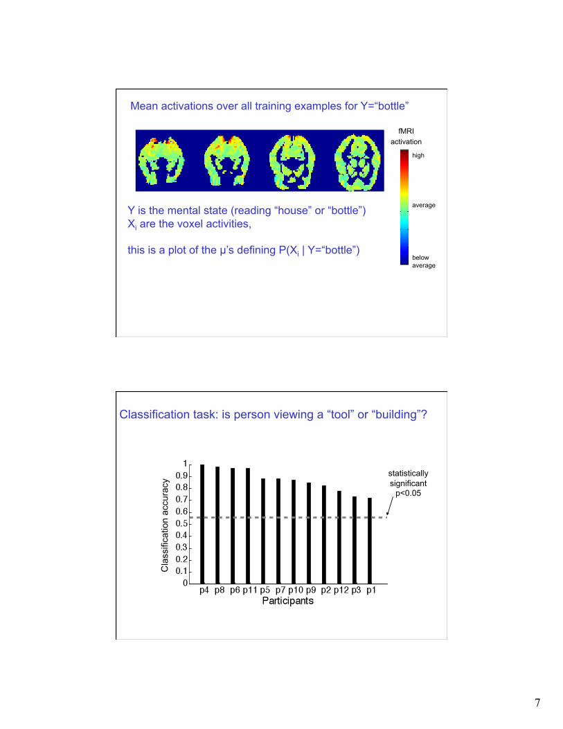
Y is the mental state (reading “house” or “bottle”) Xi are the voxel activities,

this is a plot of the µ’s defining P(Xi | Y=“bottle”)

fMRI activation

high

below average

average

Mean activations over all training examples for Y=“bottle”

Classification task: is person viewing a “tool” or “building”?

statistically significant

p<0.05

Cla

ssifi

catio

n ac

cura

cy

8

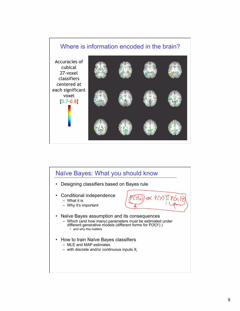
Where is information encoded in the brain?

Accuracies of cubical 27-voxel classifiers

centered at each significant

voxel [0.7-0.8]

Naïve Bayes: What you should know •  Designing classifiers based on Bayes rule

•  Conditional independence –  What it is –  Why it’s important

•  Naïve Bayes assumption and its consequences –  Which (and how many) parameters must be estimated under

different generative models (different forms for P(X|Y) ) •  and why this matters

•  How to train Naïve Bayes classifiers –  MLE and MAP estimates –  with discrete and/or continuous inputs Xi

9

Questions to think about: •  Can you use Naïve Bayes for a combination of

discrete and real-valued Xi?

•  How can we easily model just 2 of n attributes as dependent?

•  What does the decision surface of a Naïve Bayes classifier look like?

•  How would you select a subset of Xi’s?

Logistic Regression

Machine Learning 10-701

Tom M. Mitchell Machine Learning Department

Carnegie Mellon University

January 25, 2010

Required reading: •  Mitchell draft chapter (see course website) Recommended reading: •  Bishop, Chapter 3.1.3, 3.1.4 •  Ng and Jordan paper (see course website)

10

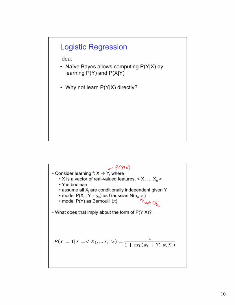
Logistic Regression Idea: •  Naïve Bayes allows computing P(Y|X) by

learning P(Y) and P(X|Y)

•  Why not learn P(Y|X) directly?

•  Consider learning f: X Y, where •  X is a vector of real-valued features, < X1 … Xn > •  Y is boolean •  assume all Xi are conditionally independent given Y •  model P(Xi | Y = yk) as Gaussian N(µik,σi) •  model P(Y) as Bernoulli (π)

•  What does that imply about the form of P(Y|X)?

11

Derive form for P(Y|X) for continuous Xi

Very convenient!

implies

implies

implies

12

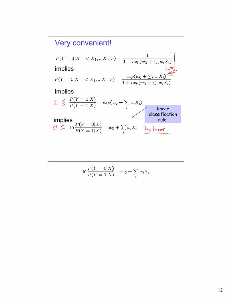
Very convenient!

implies

implies

implies

linear classification

rule!

13

Logistic function

Logistic regression more generally •  Logistic regression in more general case,

where y ∈ {y1 ... yR} : learn R-1 sets of weights

for k<R

for k=R

14

Training Logistic Regression: MCLE •  we have L training examples:

•  maximum likelihood estimate for parameters W

•  maximum conditional likelihood estimate

Training Logistic Regression: MCLE •  Choose parameters W=<w0, ... wn> to

maximize conditional likelihood of training data

•  Training data D = •  Data likelihood = •  Data conditional likelihood =

where

15

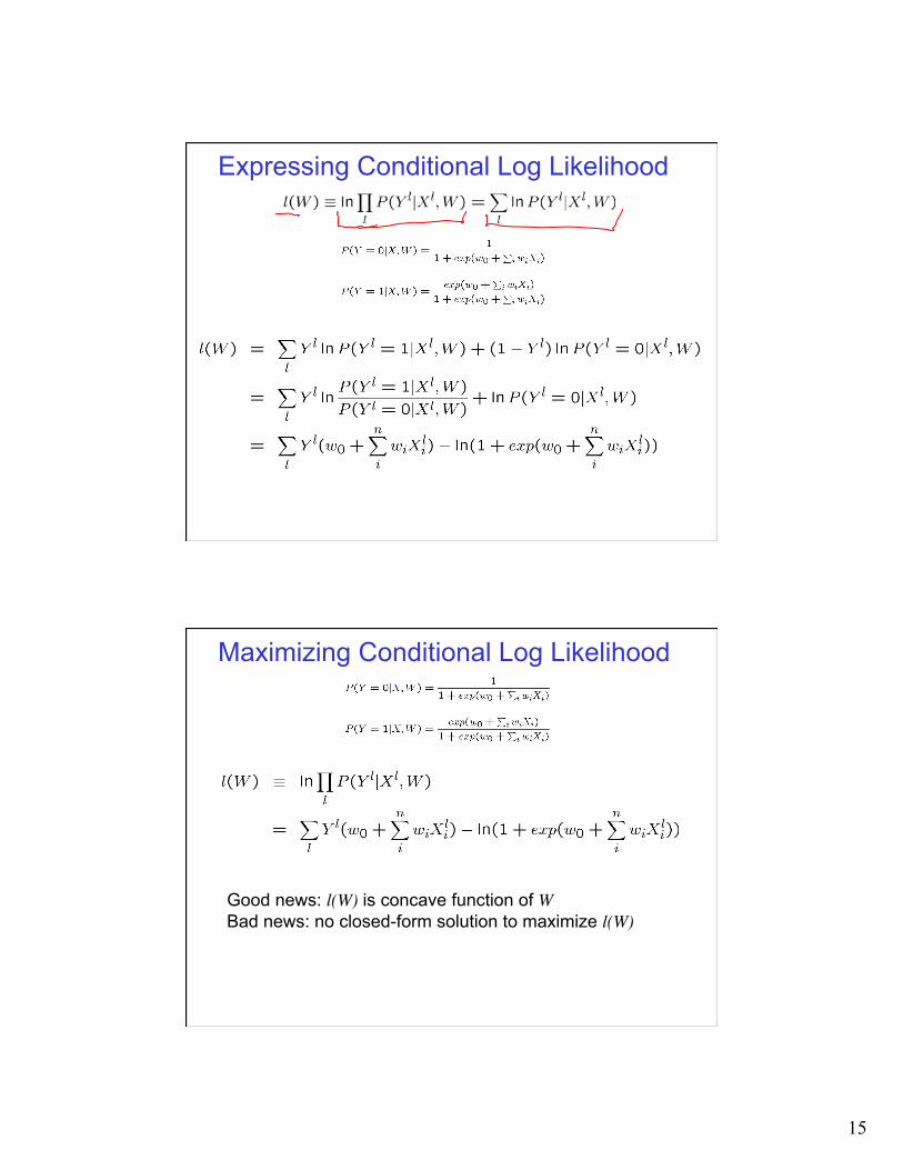
Expressing Conditional Log Likelihood

Maximizing Conditional Log Likelihood

Good news: l(W) is concave function of W Bad news: no closed-form solution to maximize l(W)

16

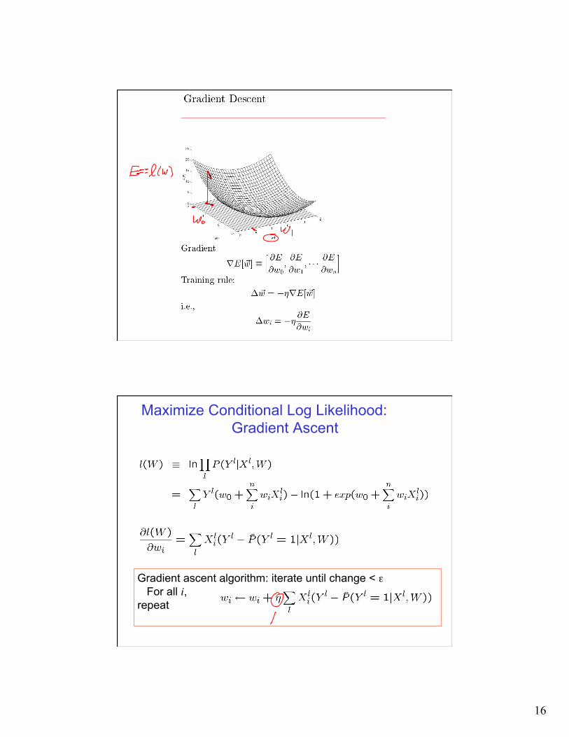
Maximize Conditional Log Likelihood: Gradient Ascent

Gradient ascent algorithm: iterate until change < ε For all i, repeat

17

That’s all for M(C)LE. How about MAP?

•  One common approach is to define priors on W –  Normal distribution, zero mean, identity covariance

•  Helps avoid very large weights and overfitting •  MAP estimate

•  let’s assume Gaussian prior: W ~ N(0, σ)

MLE vs MAP •  Maximum conditional likelihood estimate

•  Maximum a posteriori estimate with prior W~N(0,σI)

18

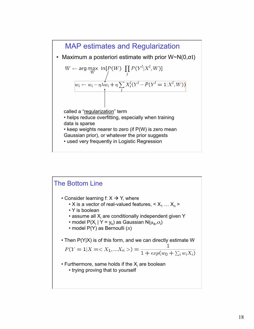
MAP estimates and Regularization •  Maximum a posteriori estimate with prior W~N(0,σI)

called a “regularization” term •  helps reduce overfitting, especially when training data is sparse •  keep weights nearer to zero (if P(W) is zero mean Gaussian prior), or whatever the prior suggests •  used very frequently in Logistic Regression

•  Consider learning f: X Y, where •  X is a vector of real-valued features, < X1 … Xn > •  Y is boolean •  assume all Xi are conditionally independent given Y •  model P(Xi | Y = yk) as Gaussian N(µik,σi) •  model P(Y) as Bernoulli (π)

•  Then P(Y|X) is of this form, and we can directly estimate W

•  Furthermore, same holds if the Xi are boolean •  trying proving that to yourself

The Bottom Line