GAS-LIQUID REACTIONS

INFLUENCE OF LIQUID BULK AND MASS TRANSFER ON PROCESS PERFORMANCE

GAS-LIQUID REACTIONS

INFLUENCE OF LIQUID BULK AND MASS TRANSFER ON PROCESS PERFORMANCE

PROEFSCHRIFT

ter verkrijging van de graad van doctor aan de Universiteit Twente,

op gezag van de rector magnificus, prof.dr. F.A. van Vught,

volgens besluit van het College voor Promoties in het openbaar te verdedigen

op vrijdag 19 oktober 2001 te 16.45 uur

door

Edwin Pieter van Elk

Geboren op 15 september 1971 te Poortugaal

Dit proefschrift is goedgekeurd door de promotor

prof.dr.ir. G.F. Versteeg

en de referent

dr.ir. P.C. Borman

DSM Research, Shell Global Solutions International and Procede Twente BV supported parts of the research presented in this thesis. © October 2001 E.P. van Elk, Doetinchem, The Netherlands

No part of this book may be reproduced in any form by print, photoprint, microfilm or any other means without written permission from the author / publisher. Niets uit deze uitgave mag worden verveelvoudigd en / of openbaar gemaakt door middel van druk, fotokopie, microfilm of op welke andere wijze dan ook zonder voorafgaande schriftelijke toestemming van de schrijver / uitgever.

Elk, Edwin Pieter van Gas-liquid reactions – Influence of liquid bulk and mass transfer on process performance – Thesis Twente University – With index, references and summary in Dutch ISBN 90 – 365 16498 Key words: mass transfer; penetration theory; reactor model; limit cycles; bifurcation

7

Contents

Contents 7

Summary 11

Samenvatting 15

1. General introduction 21 1. Gas-liquid contactors .......................................................................................................23 2. Gas-liquid mass transfer..................................................................................................23 3. This thesis ..........................................................................................................................24

3.1 Systems without the presence of a well-mixed liquid bulk ......................25 3.2 Systems with the presence of a liquid bulk..................................................25 3.3 Limit cycles .......................................................................................................26

References ................................................................................................................................26

2. Applicability of the penetration theory for gas -liquid mass transfer in

systems without a liquid bulk 29 Abstract.....................................................................................................................................30 1. Introduction.......................................................................................................................31 2. Theory ................................................................................................................................31

2.1 Introduction.......................................................................................................31 2.2 Higbie penetration model................................................................................32 2.3 Extension of penetration model for systems without liquid bulk ............34 2.4 Velocity profile .................................................................................................35 2.5 Mass transfer flux.............................................................................................35 2.6 Numerical treatment ........................................................................................36

3. Results................................................................................................................................36 3.1 Introduction.......................................................................................................36 3.2 Physical absorption..........................................................................................37 3.3 Absorption and irreversible 1,0-reaction......................................................42 3.4 Absorption and irreversible 1,1-reaction......................................................47

4. Design implications.........................................................................................................53 5. Conclusions.......................................................................................................................54

Contents

8

Acknowledgement.................................................................................................................. 55 Notation.................................................................................................................................... 55 References................................................................................................................................ 57

3. Implementation of the penetration model in dynamic modelling of gas -

liquid processes with the presence of a liquid bulk 59 Abstract .................................................................................................................................... 60 1. Introduction...................................................................................................................... 61 2. Theory ............................................................................................................................... 63

2.1 Introduction ...................................................................................................... 63 2.2 Micro model ..................................................................................................... 63 2.3 Macro model..................................................................................................... 65 2.4 Overall reactor model ..................................................................................... 66 2.5 Enhancement factor and utilisation factor................................................... 69

3. Numerical treatment........................................................................................................ 70 4. Validation results............................................................................................................. 71

4.1 Introduction...................................................................................................... 71 4.2 Physical absorption......................................................................................... 72 4.3 Equilibrium reaction in a batch reactor........................................................ 74 4.4 Absorption and irreversible 1,0-reaction..................................................... 76

5. Applications...................................................................................................................... 79 5.1 Introduction...................................................................................................... 79 5.2 Absorption and irreversible 1,0-reaction..................................................... 80 5.3 Absorption and irreversible 1,1-reaction..................................................... 82 5.4 Instantaneous reaction without enhancement............................................. 88 5.5 Equilibrium reaction ....................................................................................... 90

6. Conclusions...................................................................................................................... 91 Acknowledgement.................................................................................................................. 92 Notation.................................................................................................................................... 92 References................................................................................................................................ 95

4. Stability and dynamic behaviour of gas -liquid mass trans fer accompanied by irreversible reaction 99

Abstract .................................................................................................................................. 100 1. Introduction.................................................................................................................... 101

Contents

9

1.1 Single phase systems .....................................................................................101 1.2 Gas-liquid systems .........................................................................................101

2. Theory ..............................................................................................................................103 2.1 Introduction.....................................................................................................103 2.2 Rigorous model ..............................................................................................103 2.3 Simple model (2 ODE’s) and perturbation analysis.................................106 2.4 Approximate model (3 ODE’s) and bifurcation analysis ........................108

3. Results..............................................................................................................................110 3.1 Introduction.....................................................................................................110 3.2 Case 1 and 2 (rigorous model) .....................................................................112 3.3 Case 1 and 2 (simple model) ........................................................................113 3.4 Case 1 and 2 (approximate model)..............................................................114 3.5 Case 3 and 4 (rigorous and approximate model) ......................................116 3.6 Case 5 and 6 (rigorous and approximate model) ......................................118

4. Conclusions.....................................................................................................................120 Acknowledgement ................................................................................................................121 Notation ..................................................................................................................................121 References ..............................................................................................................................123

5. Stability and dynamic behaviour of a hydroformylation reactor –

Influence of mass transfer in the kinetics controlled regime 127 Abstract...................................................................................................................................128 1. Introduction.....................................................................................................................129 2. Theory ..............................................................................................................................130

2.1 Introduction.....................................................................................................130 2.2 Rigorous model ..............................................................................................131 2.3 Bifurcation analysis .......................................................................................134 2.4 Approximate model (4 ODE’s)....................................................................135 2.5 Saturation and utilisation ..............................................................................137

3. Results..............................................................................................................................138 3.1 Introduction.....................................................................................................138 3.2 Steady state utilization, saturation and conversion...................................139 3.3 Bifurcation analysis (approximate model).................................................141 3.4 Dynamic system behaviour..........................................................................142

4. Conclusions.....................................................................................................................146

Contents

10

Acknowledgement................................................................................................................ 146 Notation.................................................................................................................................. 147 References.............................................................................................................................. 148

6. The influence of staging on the stability of gas -liquid reactors 151 Abstract .................................................................................................................................. 152 1. Introduction.................................................................................................................... 153 2. Theory ............................................................................................................................. 153

2.1 Introduction.................................................................................................... 153 2.2 Approximate model and bifurcation analysis ........................................... 154

3. Results ............................................................................................................................. 156 3.1 Introduction.................................................................................................... 156 3.2 Single reactor (configuration 1 and 5) ....................................................... 157 3.3 Two reactors in series (configuration 2, 3 and 4)..................................... 158 3.4 Results overview............................................................................................ 160 3.5 Discussion....................................................................................................... 162

4. Conclusions.................................................................................................................... 162 Acknowledgement................................................................................................................ 163 Notation.................................................................................................................................. 163 References.............................................................................................................................. 165

Publications 167

Dankwoord 169

Levensloop 173

11

Summary Many important chemical processes involve mass transfer of one or more species from the gaseous phase to the liquid phase. In the liquid phase the species from the gas phase are converted by a chemical reaction with species already present in the liquid phase. Typical examples of industrially important processes where this phenomenon is found include gas purification, oxidation, chlorination, hydrogenation and hydroformylation processes. In behalf of the design of new reactors and the optimisation of existing reactors, advanced reactor models are required. In general, models of gas-liquid contactors consist of two main parts: the micro model and the macro model respectively. The micro model describes the interphase mass transfer between gas and liquid phase and the macro model describes the mixing behaviour in both phases. Both parts of the overall model can be solved sequential, but solving micro and macro model simultaneously is preferred because of optimisation of computational time. The phenomenon of gas-liquid mass transfer is not new and has been intensively studied by scientists in the past (the stagnant film model was first described in 1923 (W.G. Whitman, Chem. Metall. Eng. 29)). Despite of this, it was concluded that some phenomena of gas-liquid mass transfer can be regarded as nearly completely unexplained. In this thesis some of these phenomena have been studied. The Higbie penetration micro model is used as a basis for the development of some new reactor models in this thesis. The influence of the liquid bulk on the mass transfer has been studied. Special attention has been paid to the dynamical behaviour and stability of gas-liquid reactors and the influence of mass transfer limitations on the dynamics. Also, some important differences between the results of the Higbie penetration model and the stagnant film model are illustrated. Analytical solution of micro models for mass transfer accompanied by chemical reaction is restricted to asymptotic cases in which many simplifying assumptions had to be made (e.g. reaction kinetics are simple and the rate of the reaction is either very fast or very slow compared to the mass transfer). For all other situations numerical techniques are required for solving the coupled mass balances of the micro model. In

Summary

12

this thesis mostly numerical solution techniques have been applied. Where possible, analytical solutions of asymptotic cases have been used to check the validity of the numerical solution method. By modifying one of the boundary conditions of the Higbie penetration model it has been studied how the mass transfer can be affected by the presence of the liquid bulk. In a packed column the liquid flows as a thin layer over the structured or dumped packing. It has been examined whether or not the penetration model can be applied for these situations. Both physical absorption and absorption accompanied by first and second order chemical reaction have been investigated. From model calculations it is concluded that the original penetration theory, with assuming the presence of a well-mixed liquid bulk, can be applied also to systems where no liquid bulk is present, provided that the liquid layer has sufficient thickness.

For packed columns this means, in terms of Sherwood number, Sh≥4 for both physical absorption and absorption accompanied by a first order reaction. In case of a second

order 1,1-reaction a second criterion Sh≥4 ab DD / has to be fulfilled. For very thin

liquid layers (Sh<4 or Sh<4 ab DD / ), the original penetration model may give

erroneous results, depending on the exact physical and chemical parameters, and the modified model is required. Most numerical models of gas-liquid reactors make use of the physically less realistic stagnant film model because implementation of the stagnant film model is relatively easy using the Hinterland concept1. The combination of stagnant film model and Hinterland concept can successfully predict many phenomena of gas-liquid reactors. The Higbie penetration model is however preferred as a micro model because it is physically more realistic. Direct implementation of the Hinterland concept is not possible with the Higbie penetration model. In this thesis advanced numerical techniques have been applied to develop a new model that implements the Higbie

1 The Hinterland concept assumes the reaction phase to consist of a stagnant film and a well-mixed bulk. Inflow and outflow of species to and from the reactor proceeds via the non-reaction phase or via the bulk of the reaction phase, but never via the stagnant film.

Summary

13

penetration model for the phenomenon mass transfer accompanied by chemical reaction in well-mixed two-phase reactors. By comparing the model results with analytical asymptotic solutions it is concluded that the model predicts the reactor satisfactorily. It is shown that for many asymptotic cases the results of this new model coincide with the results of the stagnant film model with Hinterland concept. For some special conditions, differences can exist between the results obtained using the stagnant film model with Hinterland concept and the implementation of the Higbie penetration model. An important result is that for 1,1-reactions the saturation of the liquid phase with gas phase species does not approach zero with increasing reaction rate (increasing Hatta number), contrary to what is predicted by the film model with Hinterland concept. Another important deviation can be found at the specific conditions of a so-called instantaneous reaction in combination

with the absence of chemical enhancement of mass transfer (Ha>>Ea∞ and Ea∞=2). Application of the penetration model does not provide any numerical difficulties, while application of the stagnant film model would lead to a discontinuity in the concentration gradient. Another disadvantage of the Hinterland concept is that it can strictly only be applied to isothermal systems, whereas in the systems investigated in this thesis the reaction enthalpy is an important parameter that may significantly influence the phenomena of gas-liquid mass transfer. In this thesis a rigorous model has been developed that simulates the dynamic behaviour of stirred non-isothermal gas-liquid reactors by simultaneously solving the Higbie penetration model for the phenomenon mass transfer accompanied by chemical reaction and the dynamic gas and liquid phase component and heat balances. This is achieved by coupling the ordinary differential equations of the macro model mass and heat balances to the partial differential equations of the penetration model. Such a model has not been published in literature before, but results in a very reliable dynamic reactor model that can be applied over a wide range of conditions. Using the newly developed rigorous reactor model it is shown that dynamic instability (limit cycles) can occur in gas-liquid reactors. The influence of mass transfer limitations on these limit cycles has been studied and is has been found that mass transfer limitations make the process more stable.

Summary

14

Although the rigorous model is believed to be a very accurate model, it has the disadvantage that due to the complex numerical methods applied it is a time-consuming model. In behalf of a more efficient prediction of the possible occurrence of limit cycles, the reactor model was simplified. The simplified model is suited for the prediction of limit cycles using a stability analysis. A stability analysis is a very efficient method to predict the dynamic behaviour and stability of a system of ordinary differential equations by linearisation of the governing non-linear ODE’s in the neighbourhood of the steady state and analysing the Eigenvalues. This method is very powerful for attaining design rules for stable operation of stirred gas-liquid reactors. The influence of mass transfer limitations on the limit cycles is predicted very well using the simplified model, though small discrepancies are found with the more accurate rigorous model. The developed reactor models have been used to model the dynamics of a new, to be developed, industrial hydroformylation reactor. At a certain design of the reactor, the model predicts serious and undesired limit cycles. These conditions have to be avoided by an appropriate reactor design. Hydroformylation reactions are often characterised by a negative reaction order in carbon monoxide. Model calculations described in this thesis show that this can lead to interesting phenomena: at certain process conditions, an improvement of the mass transfer (higher kla, for example due to better mixing) can give rise to a less stable reactor, without increasing the conversion. This unusual phenomenon is explained by the negative reaction order of carbon monoxide. Apparently, the increasing hydrogen and carbon monoxide concentrations cancel each other out and the overall reaction rate remains unchanged. The increasing hydrogen and carbon monoxide concentrations do however make the process more sensitive for the occurrence of limit cycles. Finally, a start has been made with studying the influence of macro-mixing on the dynamical behaviour of gas-liquid reactors. For this purpose a cascade of two reactors in series is compared to a single reactor. The first results indicate that a cascade of reactors in series provides a dynamically more stable design. The total required cooling surface to prevent the occurrence of temperature-concentration limit cycles decreases significantly with increasing number of reactors in series. The first reactor in the cascade is the one with the highest risk of dynamic instability.

15

Samenvatting Een aantal belangrijke chemische processen wordt gekenmerkt door stofoverdracht van een of meerdere componenten van de gasfase naar een vloeistoffase. In de vloeistoffase vindt vervolgens een chemische reactie plaats tussen de uit de gasfase afkomstige component(en) en een reeds in de vloeistoffase aanwezige component. Enkele voorbeelden van industrieel belangrijke processen waarbij dit verschijnsel zich voordoet zijn: gas-zuivering, oxidatie, chlorering, hydrogenering en hydroformylering. Ten behoeve van het ontwerpen van nieuwe reactoren en het optimaliseren van bestaande reactoren zijn geavanceerde reactormodellen noodzakelijk. Modellen van gas-vloeistof contactapparaten bestaan in het algemeen uit twee afzonderlijke delen, te weten het micromodel en het macromodel. Het micromodel beschrijft de stofoverdracht tussen gas en vloeistof, terwijl het macro model het menggedrag in beide fasen beschrijft. Beide delen worden sequentieel of bij voorkeur simultaan opgelost en vormen zo het reactormodel. Het optreden van gas-vloeistof stofoverdracht wordt reeds geruime tijd wetenschappelijk bestudeerd (het film model dateert uit 1923 (W.G. Whitman, Chem. Metall. Eng. 29)). Desondanks zijn er nog diverse fenomenen niet volledig verklaard. In dit proefschrift wordt een aantal van deze fenomenen bestudeerd. Als micromodel wordt gebruik gemaakt van het Higbie penetratiemodel bij de ontwikkeling van een aantal nieuwe reactormodellen. De invloed van de vloeistofbulk op de stofoverdracht wordt bestudeerd. Bijzondere aandacht wordt geschonken aan het dynamisch gedrag en de dynamische stabiliteit van gas-vloeistof reactoren en hoe dit wordt beïnvloed door het optreden van stofoverdrachtslimiteringen. Daarnaast worden enkele verschillen tussen het Higbie penetratiemodel en het stagnante film model belicht. Analytische uitwerking van met name de micro-modellen is beperkt tot een aantal eenvoudige situaties (onder meer zeer eenvoudig reactie-mechanisme en zeer hoge of juist zeer lage reactiesnelheid in relatie tot de stofoverdrachtssnelheid). In dit proefschrift is grotendeels gebruik gemaakt van numerieke methodes om de modellen op te lossen. Ter controle zijn, waar mogelijk, limitsituaties vergeleken met analytische oplossingen om zo de numerieke oplosmethodes te controleren.

Samenvatting

16

Door aanpassing van één van de randvoorwaarden van het penetratiemodel is bestudeerd of, onder welke omstandigheden en in welke mate de absorptiesnelheid wordt beïnvloed door de aanwezigheid van de vloeistofbulk. In een gepakte kolom kan de vloeistof bijvoorbeeld in een dunne laag over de gestructureerde of gestorte pakking stromen. Onderzocht is of in dergelijke situaties het penetratiemodel nog toegepast kan worden. Fysische absorptie alsmede door 1,0- en 1,1-reacties chemisch versnelde stofoverdracht is bestudeerd. Uit de modelberekeningen blijkt dat het penetratiemodel met de aanname van de aanwezigheid van een goed gemengde vloeistofbulk ook kan worden toegepast bij afwezigheid van zo’n vloeistofbulk, mits de dikte van de vloeistoflaag een bepaalde minimaal benodigde waarde heeft. Voor gepakte kolommen kan dit worden uitgedrukt

in een Sherwood-criterium. Indien Sh≥4 kan het penetratiemodel worden toegepast voor fysische absorptie of absorptie met 1,0-reactie. Bij 1,1-reacties geldt een aanvullende eis

dat Sh≥4 ab DD / . Indien aan deze criteria niet wordt voldaan dan kan de berekende

absorptiesnelheid hoger zijn dan de werkelijke absorptiesnelheid. Ten behoeve van de modellering van geroerde gas-vloeistof reactoren wordt, mede door de relatief eenvoudige implementatie, veelal gebruik gemaakt van het film model in combinatie met het Achterland concept1. Deze combinatie kan in veel situaties succesvol worden toegepast, doch het penetratie model en het surface renewal model zijn fysisch meer realistisch en verdienen derhalve de voorkeur boven het film model. Directe toepassing van het Achterland concept in combinatie met het penetratie model is echter niet mogelijk. In dit proefschrift wordt gebruik gemaakt van geavanceerde numerieke technieken ten behoeve van de ontwikkeling van een nieuw model waarin het Higbie penetratiemodel voor stofoverdracht met chemische reactie in goed gemengde gas-vloeistof reactoren is geïmplementeerd.

1 Het Achterland concept veronderstelt dat de reactiefase bestaat uit een stagnante film en een goed gemengde bulk. Instroom en uitstroom van componenten naar en van de reactor verloopt via de niet-reactiefase of via de bulk van de reactiefase, doch nooit via de stagnante film.

Samenvatting

17

De resultaten van het model komen in limietsituaties grotendeels overeen met de resultaten verkregen met de combinatie van film model en Achterland concept. Er is echter ook een aantal specifieke condities waarbij de resultaten van het nieuw ontwikkelde model significant anders zijn dan de resultaten verkregen met bestaande modellen. Een belangrijk resultaat is dat voor 1,1-reacties de verzadiging van de vloeistoffase met de gasfasecomponent niet naar nul convergeert met toenemende reactiesnelheid (toenemend Hatta kental) terwijl dit volgens het film model met Achterland concept wel zo is. Een andere bijzonderheid treedt op onder de specifieke omstandigheden waarbij een zogenaamde instantane reactie optreedt in combinatie met

de afwezigheid van chemische versnelling (Ha>>Ea∞ and Ea∞=2). Toepassing van het penetratiemodel geeft hier geen enkele moeilijkheid terwijl de toepassing van het film model resulteert in een discontinuïteit in de concentratiegradiënt. Een ander nadeel van het Achterland concept is dat het een isotherm model is, terwijl bij de systemen welke in dit proefschrift zijn bestudeerd de reactie-enthalpie een belangrijke parameter is die van grote invloed kan zijn op de verkregen resultaten. In dit proefschrift is derhalve een rigoureus model ontwikkeld waarmee het penetratie model en het geroerde tank model simultaan worden opgelost door koppeling van de differentiaal vergelijkingen van de massa- en energiebalansen van het geroerde tank model aan de partiele differentiaal vergelijkingen van het penetratiemodel. Dit resulteert in een geavanceerd en uiterst betrouwbaar dynamisch reactormodel dat niet eerder in de literatuur beschreven is. Met behulp van het rigoureuze reactormodel is aangetoond dat dynamische instabiliteit (oscillaties) kan optreden in gas-vloeistof reactoren. Onderzocht is eveneens hoe deze oscillaties worden beïnvloed door stofoverdrachtslimiteringen. Het blijkt dat eventuele stofoverdrachtslimiteringen het systeem stabieler maken. Hoewel het rigoureuze model een zeer nauwkeurig model is, heeft het wel het nadeel dat het als gevolg van de grote hoeveelheid gekoppelde (partiele) differentiaal vergelijkingen een tijdrovend model is. Voor een efficiëntere voorspelling van de oscillaties is het reactormodel vereenvoudigd. Dit vereenvoudigde model blijkt succesvol te kunnen worden ingezet om het optreden van oscillaties te voorspellen door middel van een stabiliteitsanalyse. Een stabiliteitsanalyse is een zeer efficiënte methode om het dynamisch gedrag en de stabiliteit van een systeem van gewone differentiaal

Samenvatting

18

vergelijkingen (DV) te voorspellen door middels van een linearisatie van de niet-lineaire DV’s in de nabijheid van de stationaire toestand gevolgd door een analyse van de Eigenwaarden. De invloed van stofoverdrachtslimiteringen op de oscillaties wordt door het vereenvoudigde model goed voorspelt, hoewel er kleine verschillen bestaan ten opzichte van de resultaten verkregen met het rigoureuze model. De nieuwe modellen zijn gebruikt om het dynamisch gedrag van een nieuw te ontwerpen industriële hydroformyleringsreactor te bestuderen. Onder bepaalde ontwerpcondities voorspelt het model ongewenste oscillaties. Deze condities dienen derhalve vermeden te worden bij het reactorontwerp. Hydroformyleringsreacties hebben vaak een negatieve reactieorde in koolmonoxide. Uit modelberekeningen blijkt dat dit onder specifieke omstandigheden kan leiden tot interessante verschijnselen: een verbetering van de stofoverdracht (hogere kla, bijvoorbeeld door harder te roeren) kan in een specifiek regime leiden tot een minder stabiele reactor, terwijl de conversie niet verandert of zelfs kan dalen. Dit ongewone verschijnsel kan worden verklaard door de negatieve reactieorde in koolmonoxide. Klaarblijkelijk heffen de toenemende concentraties van waterstof en koolmonoxide elkaar op en blijft de resulterende reactiesnelheid onveranderd. De toenemende concentraties van waterstof en koolmonoxide maken het proces echter wel gevoeliger voor het optreden van oscillaties. Tot slot is een eerste aanzet gegeven om de invloed van macro-menging op het dynamisch gedrag van gas-vloeistof reactoren te bestuderen. Hiertoe is een cascade van twee reactoren in serie vergeleken met een enkele reactor. De eerste resultaten wijzen erop dat het plaatsen van meerdere reactoren in serie resulteert in een dynamisch stabieler ontwerp. Het totaal benodigde koeloppervlak om temperatuuroscillaties te voorkomen is aanzienlijk kleiner bij plaatsing van reactoren in serie. De grootste risico’s voor instabiliteit treden op in de eerste reactor in de cascade.

19

20

21

CHAPTER 1

General introduction

1. General introduction

Chapter 1

22

Chapter 1

23

1. Gas-liquid contactors Gas-liquid contactors are frequently encountered in chemical process industry. In these contactors a gas phase and a liquid phase are brought into contact with each other and mass transfer between the gas and the liquid phase takes place. Often, but not necessarily, the mass transfer is accompanied by the simultaneous occurrence of a chemical reaction. A good understanding of the behaviour of gas-liquid contactors is essential for design purposes. Gas-liquid contactors exist in a number of configurations. Mass transfer can take place from the gas phase to the liquid phase as well as from the liquid phase to the gas phase. Chemical reactions may occur in the gas and/or in the liquid phase respectively. Gas and liquid phases can have various mixing patterns (plug flow, well stirred, plug flow with axial dispersion, etc.). This thesis focuses on gas-liquid contactors where one or more species are transferred from the gas phase to the liquid phase, optionally followed by a chemical reaction in the liquid phase. Industrially important examples of such gas-liquid processes include gas purification, oxidation, chlorination, hydrogenation and hydroformylation processes. Chapter 2 of this thesis focuses on gas-liquid contactors without the presence of a liquid bulk. Chapter 3 to 6 focus on gas-liquid reactors with the presence of a well-stirred liquid bulk.

2. Gas-liquid mass transfer A numerical model of a gas-liquid contactor typically consists of two main parts: the micro model, describing the mass transfer between the gas and the liquid phase and the macro model describing the mixing pattern within the individual gas and liquid phases. Frequently applied micro models include: 1. The stagnant film model (Whitman, 1923). 2. The Higbie penetration model (Higbie, 1935). 3. The Danckwerts surface renewal model (Danckwerts, 1951). 4. The film penetration model (Dobbins, 1956 and Toor & Marchello, 1958).

Chapter 1

24

The stagnant film model assumes the presence of a stagnant liquid film, while the penetration model and the surface renewal model approach the gas-liquid mass transfer using dynamic absorption in small liquid elements at the contact surface. In this thesis the Higbie penetration model is selected because: 1. As pointed out by Westerterp et al. (1990) and Versteeg et al. (1987) the Higbie

penetration model is physically more realistic than the stagnant film model. 2. Chapter 3 to 6 of this thesis go into the subject of modelling the dynamic behaviour

of gas-liquid reactors. The stagnant film model is not a dynamic model and thus less suited for modelling dynamic processes. The Higbie penetration model is a dynamic micro model and can be applied in dynamic models.

3. In this thesis some phenomena are described for which the stagnant film model may fail or at least be less accurate.

4. The Higbie penetration model was favoured to the Danckwerts surface renewal model because the Higbie penetration model is easier to implement and can describe all phenomena discussed in this thesis.

3. This thesis Gas-liquid mass transfer has been studied scientifically for a long period of time (the stagnant film model was first published in 1923 by Whitman). In spite of this, there still exist no satisfactory design criteria for all phenomena of gas-liquid mass transfer that may occur. This is mainly due to restrictions in mathematically solving the governing compound or mass balances. However, modern computer technology now makes it possible to numerically solve these complex models. In this thesis, the following phenomena of gas-liquid mass transfer are discussed: 1. In Chapter 2, the influence of the absence of a liquid bulk on the mass transfer flux

is studied. 2. In Chapter 3, the implementation of the penetration model in dynamic macro

models for ideally stirred gas-liquid reactors is described. This chapter also discusses some differences between the penetration model and the stagnant film model.

3. In Chapters 4 to 6, the influence of gas-liquid mass transfer on the dynamic stability of gas-liquid reactors is described.

Chapter 1

25

3.1 Systems without the presence of a well-mixed liquid bulk

One of the boundary conditions of the penetration model is that the concentration gradient at infinite distance of the mass transfer surface is equal to zero. This boundary condition restricts the applicability of the penetration model to systems with a sufficiently large liquid bulk (Versteeg et al., 1989). Some gas-liquid contactors are characterised by the absence of a liquid bulk, a very thin layer of liquid flows over a solid surface. An example of such a contactor is an absorption column equipped with structured packing elements. In Chapter 2 of this thesis, the boundary conditions of the penetration model are modified such that the penetration theory can be applied to systems where no liquid bulk is present. The differences with systems with a liquid bulk are discussed and criteria for application of the penetration model are given. This work is for example important for the modelling of CO2 and/or H2S absorption in gas treatment with aqueous amine solutions in packed columns as pointed out by Knaap et al. (2000). 3.2 Systems with the presence of a liquid bulk

In modelling of well-mixed gas-liquid reactors, the most frequently applied micro model is the stagnant film model. Implementation of the stagnant film model in the overall reactor model is relatively easy using the Hinterland concept (see Westerterp et al., 1990), although only applied to first order irreversible reactions. In literature no model has been presented with which the Higbie penetration model is implemented as part of a dynamic overall gas-liquid reactor model, therefore such a model has been developed in this thesis. In Chapter 3 the new model, where the Higbie penetration model is implemented in a dynamic macro model of well-mixed gas-liquid reactors, is presented. This results in a very reliable and widely applicable reactor model based on the physically realistic penetration theory. Although in most situations it is found that the new model gives similar results as compared to the Hinterland concept, Chapter 3 also discusses some interesting differences between both models.

Chapter 1

26

3.3 Limit cycles

Multiplicity, stability and dynamics of single phase reactors is described intensively in literature (e.g. Westerterp et al., 1990). Analytical design rules for stable operation are available, provided that the system can be described sufficiently accurate with a system of two ordinary differential equations. An example of such a system is a cooled single phase continuously ideally stirred tank reactor (Vleeschhouwer and Fortuin, 1990). Prediction of the dynamics of ideally stirred gas-liquid reactors is more complex and only a few papers are devoted to this subject. As pointed out by Vleeschhouwer (Vleeschhouwer et al., 1992) accurate prediction of the dynamic behaviour of industrial gas-liquid reactors is very important because badly designed reactors can lead to dynamic instability (limit cycles). Generally, the occurrence of limit cycles has to be avoided, because they may adversely affect product quality, downstream operations, catalyst deactivation and can lead to serious difficulty in process control and therefore unsafe operations. One of the main incentives of this thesis was to improve the available design rules for stable operation of gas-liquid reactors. In Chapter 4 general applicable design rules for stable operation of well-mixed gas-liquid reactors are developed and validated. These design rules are an extension of the work presented by Vleeschhouwer et al. (1990). The influence of mass transfer on the occurrence of limit cycles is discussed. In Chapter 5 the stability of an industrial hydroformylation reactor is modelled. Special attention has been paid to the effect of the mass transfer coefficient on the stability and conversion of the hydroformylation process. In Chapter 6 the influence of putting more stirred gas-liquid reactors in series on the design rules is discussed.

References Danckwerts, P.V., (1951), Significance of liquid-film coefficients in gas absorption, Ind. Eng. Chem. 43, 1460-1467.

Chapter 1

27

Dobbins, W.E., (1956), in: McCable, M.L. and Eckenfelder, W.W. (Eds.), Biological treatment of sewage and industrial wastes, Part 2-1, Reinhold, New York. Higbie, R., (1935), The rate of absorption of a pure gas into a still liquid during short periods of exposure, Trans. Am. Inst. Chem. Eng. 35, 36-60. Knaap, M.C., Oude Lenferink, J.E., Versteeg, G.F. and Elk, E.P. van, (2000), Differences in local absorption rates of CO2 as observed in numerically comparing tray columns and packed columns, 79th annual Gas Processors Association convention, 82-94.

Toor, H.L. and Marchello, J.M., (1958), Film-penetration model for mass transfer and heat transfer, AIChE Journal 4, 97-101. Versteeg, G.F., Blauwhoff, P.M.M. and Swaaij, W.P.M. van, (1987), The effect of diffusivity on gas-liquid mass transfer in stirred vessels. Experiments at atmospheric and elevated pressures, Chem. Eng. Sci.42, 1103-1119. Versteeg, G.F., Kuipers J.A.M., Beckum, F.P.H. van and Swaaij, W.P.M. van, (1989), Mass transfer with complex reversible chemical reactions – I. Single reversible chemical reaction, Chem. Eng. Sci. 44, 2295-2310. Vleeschhouwer, P.H.M. and Fortuin, J.M.H., (1990), Theory and experiments concerning the stabilty of a reacting system in a CSTR, AIChE Journal 36, 961-965. Vleeschhouwer, P.H.M., Garton, R.D. and Fortuin, J.M.H., (1992), Analysis of limit cycles in an industrial oxo reactor, Chem. Eng. Sci. 47, 2547-2552. Westerterp, K.R., Swaaij, W.P.M. van and Beenackers, A.A.C.M., (1990), Chemical Reactor Design and Operation, Wiley, New York. Whitman, W.G., (1923), Preliminary experimental confirmation of the two-film theory of gas absorption, Chem. Metall. Eng. 29, 146-148.

Chapter 1

28

29

CHAPTER 2

Applicability of the penetration theory for gas-liquid

mass transfer in systems without a liquid bulk

2. Applicability of the penetration theory for gas-

liquid mass transfer in systems without a liquid bulk

Chapter 2

30

Abstract Frequently applied micro models for gas-liquid mass transfer all assume the presence of a liquid bulk. However, some systems are characterised by the absence of a liquid bulk, a very thin layer of liquid flows over a solid surface. An example of such a process is absorption in a column equipped with structured packing elements. The Higbie penetration model (Higbie, 1935) was slightly modified, so that it can describe systems without liquid bulk. A comparison is made between the results obtained with the modified model and the results that would be obtained when applying the original penetration theory for systems with a liquid bulk. Both physical absorption and absorption accompanied by first and second order chemical reaction have been investigated. It is concluded that the original penetration theory can be applied for systems without liquid bulk, provided that the liquid layer has sufficient thickness

(δ>d*pen). For packed columns this means, in terms of Sherwood number, Sh≥4. In case

of a 1,1-reaction with Ha>0.2 a second criterion is Sh≥4 ab DD / . For very thin liquid

layers (Sh<4 or Sh<4 ab DD / ), the original penetration model may give erroneous

results, depending on the exact physical and chemical parameters, and the modified model is required. Experiments are required to confirm the results found in this numerical study.

Chapter 2

31

1. Introduction Mass transfer from a gas phase to a liquid phase proceeds via the interfacial area. Micro models are required to model this interphase transport of mass that may take place in combination with a chemical reaction. Frequently applied micro models are the stagnant film model in which mass transfer is

postulated to proceed via stationary molecular diffusion in a stagnant film of thickness δ

(Whitman, 1923), the penetration model in which the residence time θ of a fluid element at the interface is the characteristic parameter (Higbie, 1935), the surface renewal model in which a probability of replacement is introduced (Danckwerts, 1951) and the film-penetration model which is a two-parameter model combining the stagnant film model and the penetration model (Dobbins, 1956 and Toor & Marchello, 1958). All micro models mentioned above assume the presence of a well-mixed liquid bulk. This may limit the application of these models to systems where a liquid bulk is present, for example absorption in a tray column or mass transfer in a stirred tank reactor. The question arises whether it is also possible to apply the micro models for systems where no liquid bulk is present, for example absorption in a column with structured or random packing elements, where thin liquid layers flow over the packing. In this chapter, the penetration model approach is adapted, so that it can describe systems without a liquid bulk. Next, a comparison is made between the results obtained with the modified model and the results that would be obtained when applying the original penetration theory for systems with a liquid bulk.

2. Theory 2.1 Introduction

The problem considered is gas-liquid mass transfer followed by an irreversible first or second order chemical reaction:

(l)(l)(l)(g) dcb DCBA γγγ +→+ (2.1)

Chapter 2

32

with the following overall reaction rate equation:

nRa BAkR ]][[= (2.2)

where γb=n=0 in case of a first order reaction and γb=n=1 in case of a second order reaction. The mathematical model used is based on the following assumptions: 1. Mass transfer of component A takes place from the gas phase to a liquid layer that

flows over a vertical contact surface (i.e. a packing or a reactor wall) 2. The mass transfer in the gas phase is described with the stagnant film model. The

conditions are chosen so that the gas phase mass transfer is no limiting factor. 3. The mass transfer in the liquid phase is described according to the penetration model

approach. 4. The reaction takes place in the liquid phase only. 5. The liquid phase components (B, C and D) are non-volatile. 6. Axial dispersion in the liquid layer can be neglected. 7. The velocity profile in the liquid layer is either plug flow or a fully developed

parabolic velocity profile (laminar flow). 8. The possible influence of temperature effects on micro scale is neglected. 2.2 Higbie penetration model

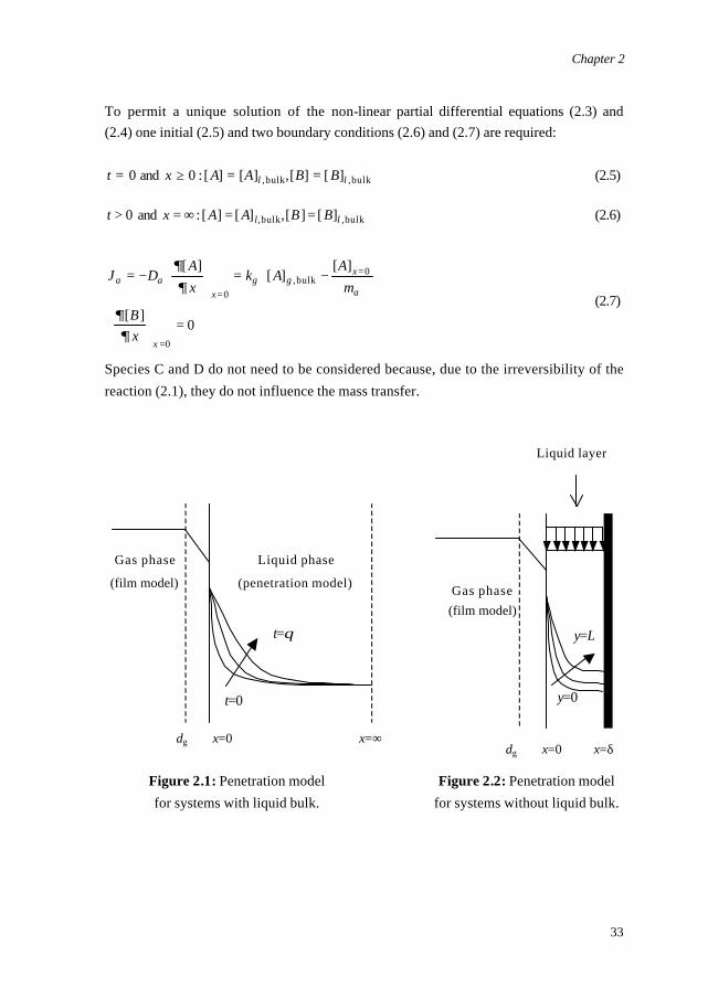
First, the standard penetration theory is discussed (Figure 2.1). The phenomenon of mass transfer accompanied by a chemical reaction is governed by the following equations:

aa RxAD

tA −=

2

2 ][][∂

∂∂

∂ (2.3)

abb RxBD

tB γ

∂∂

∂∂ −=

2

2 ][][ (2.4)

Chapter 2

33

To permit a unique solution of the non-linear partial differential equations (2.3) and (2.4) one initial (2.5) and two boundary conditions (2.6) and (2.7) are required:

bulk,bulk, ][][,][][:0and0 ll BBAAxt ==≥= (2.5)

bulk,bulk, ][][,][][:and0 ll BBAAxt ==∞=> (2.6)

0][

][][

][

0

0bulk,

0

=

−=

−=

=

=

=

x

a

xgg

xaa

xB

mA

AkxA

DJ

∂∂

∂∂

(2.7)

Species C and D do not need to be considered because, due to the irreversibility of the reaction (2.1), they do not influence the mass transfer.

Figure 2.1: Penetration model for systems with liquid bulk.

Figure 2.2: Penetration model for systems without liquid bulk.

Gas phase (film model)

Liquid layer

y=0

Gas phase

(film model)

Liquid phase

(penetration model)

δg x=0 x=∞

t=0

t=θ

δg x=0 x=δ

y=L

Chapter 2

34

2.3 Extension of penetration model for systems without liquid bulk

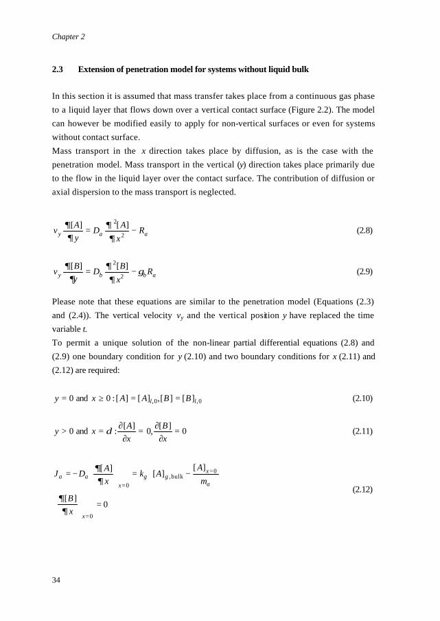
In this section it is assumed that mass transfer takes place from a continuous gas phase to a liquid layer that flows down over a vertical contact surface (Figure 2.2). The model can however be modified easily to apply for non-vertical surfaces or even for systems without contact surface. Mass transport in the x direction takes place by diffusion, as is the case with the penetration model. Mass transport in the vertical (y) direction takes place primarily due to the flow in the liquid layer over the contact surface. The contribution of diffusion or axial dispersion to the mass transport is neglected.

aay RxAD

yAv −=

2

2 ][][∂

∂∂∂ (2.8)

abby RxBD

yBv γ

∂∂

∂∂ −=

2

2 ][][ (2.9)

Please note that these equations are similar to the penetration model (Equations (2.3) and (2.4)). The vertical velocity vy and the vertical position y have replaced the time variable t. To permit a unique solution of the non-linear partial differential equations (2.8) and (2.9) one boundary condition for y (2.10) and two boundary conditions for x (2.11) and (2.12) are required:

0,0, ][][,][][:0and0 ll BBAAxy ==≥= (2.10)

0][,0][:and0 =∂

∂=∂

∂=>xB

xAxy δ (2.11)

0][

][][][

0

0bulk,

0

=

−=

−=

=

=

=

x

a

xgg

xaa

xB

mA

AkxADJ

∂∂

∂∂

(2.12)

Chapter 2

35

Please note that the boundary condition for x=∞ (Equation (2.6)) has been replaced by a

boundary condition for x=δ (Equation (2.11)). Equation (2.11) is a mathematical formulation for the fact that no species can diffuse through the solid surface. 2.4 Velocity profile

The velocity profile, required to solve the model, is limited by two extremes: 1. Plug flow, the velocity vy is independent of the position x. 2. Laminar flow with no-slip boundary condition, the velocity vy at the wall is zero.

Assuming a parabolic velocity profile vy can be calculated from

−=

2

max 1δx

vv y (2.13)

The maximum velocity vmax is found at the gas-liquid interface and can be calculated from:

µδρ

2

2

maxg

v = (2.14)

The most likely situation is that at t=0, the velocity profile is a plug flow profile. At t>0 the velocity profile gradually changes from plug flow to parabolic. The actual (average)

mass transfer flux between t=0 and t=θ will be in between the mass transfer flux for plug flow and for parabolic velocity profile depending on the contact length L. 2.5 Mass transfer flux

The mass transfer flux is calculated as the average flux over the contact time θ (penetration model) or the contact length L (layer model):

txA

DJx

aa d][1

0 0bulk, ∫

=

−=

θ

∂∂

θ (2.15)

Chapter 2

36

yxA

DL

JL

xaa d

][1

0 0layer, ∫

=

−=

∂∂

(2.16)

2.6 Numerical treatment

In the penetration theory, the concentration profiles are time-dependent: they develop a solution of a system of coupled non-linear parabolic partial differential equations subject to specified initial and two-point boundary conditions. The approach used to solve these equations is based on the method presented by Versteeg et al. (1989). However, the special error-function transformation used by Versteeg et al. was not implemented, because this can only be used for systems with a liquid bulk present.

3. Results 3.1 Introduction

The main goal of this chapter is to investigate what are the differences between the results obtained with the penetration model for systems with liquid bulk and the results obtained with the modified model for systems where a thin liquid layer flows over a vertical contact surface. Three different kinds of absorption have been investigated: physical absorption (section 3.2), absorption and irreversible 1,0 reaction (section 3.3) and finally absorption and irreversible 1,1 reaction (section 3.4). Both plug flow and parabolic velocity profiles in

the liquid layer were studied. All the important parameters ([A], [B], Da, Db, kR, δ, kl, ma, vmax) have been varied over a wide range. It was found that most results could be summarised into only a few plots, using dimensionless numbers. The important dimensionless numbers used are:

bulk,

layer,

a

a

J

J=η (2.17)

Chapter 2

37

θ

δδ

iii

DdX

4pen== (2.18)

l

an

R

k

DBkHa

][= (2.19)

ga

l

AmA

Sat][

][ 0

= (2.20)

3.2 Physical absorption

First consider physical absorption (kR=0). The analytical solution of the absorption flux for the penetration model is given by:

( )lgala AAmkJ ][][bulk, −= (2.21) As a basecase, the following conditions were taken: kl=5· 10-5 m/s, ma=0.5, [A]g=100 mol/m3, Da=1· 10-9 m2/s, plug flow velocity in layer with vy=0.1 m/s. The corresponding

penetration depth (dpen) is 45 µm. The mass transfer flux found with the modified mo del is given for layers of different thickness in Table 2.1.

Table 2.1: Mass transfer flux (mol/m2s) as a function of layer thickness, results are valid for basecase.

layer model Ja,bulk Ja,dpen Ja,dpen/2 Ja,dpen/4 Ja,dpen/8 Ja,dpen/16

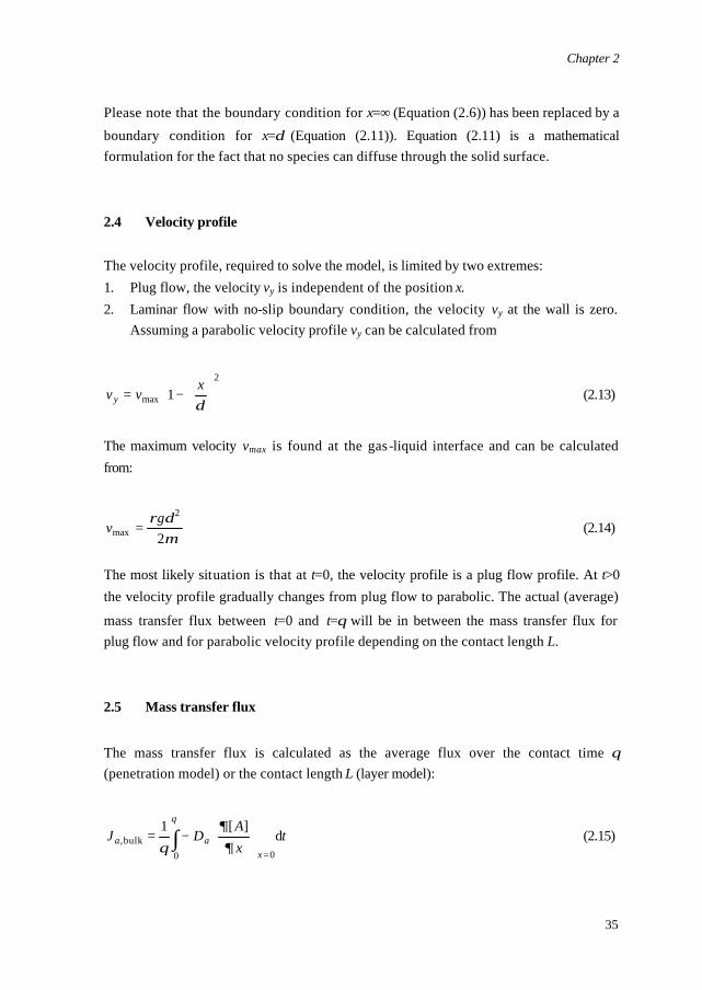
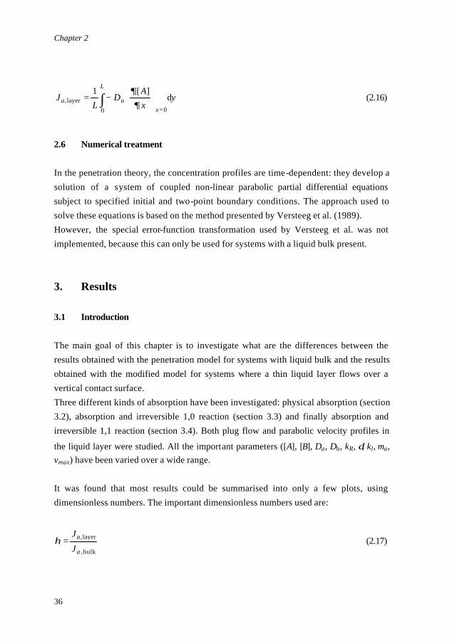
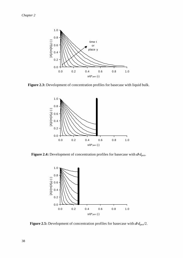
0.0025 0.00249 0.00206 0.00111 0.00055 0.00028 Figure 2.3 Figure 2.4 Figure 2.5 - - -

It is found (Table 2.1) that the mass transfer flux decreases with decreasing layer

thickness. If the layer has a thickness of at least the penetration depth (δ>dpen) the mass transfer flux approaches a value that corresponds to the mass transfer flux according to the penetration theory (Ja,dpen=Ja,bulk).

Chapter 2

38

0.0

0.2

0.4

0.6

0.8

1.0

0.0 0.2 0.4 0.6 0.8 1.0

x/d*pen (-)

[A]l/

(m[A

]g)

(-)

time tor

place y

Figure 2.3: Development of concentration profiles for basecase with liquid bulk.

0.0

0.2

0.4

0.6

0.8

1.0

0.0 0.2 0.4 0.6 0.8 1.0

x/d*pen (-)

[A]l/

(m[A

]g)

(-)

Figure 2.4: Development of concentration profiles for basecase with δ=dpen.

0.0

0.2

0.4

0.6

0.8

1.0

0.0 0.2 0.4 0.6 0.8 1.0

x/d*pen (-)

[A]l/

(m[A

]g)

(-)

Figure 2.5: Development of concentration profiles for basecase with δ=dpen/2.

Chapter 2

39

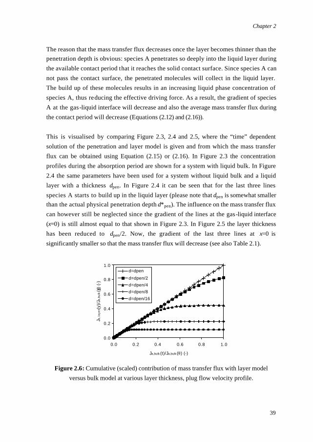
The reason that the mass transfer flux decreases once the layer becomes thinner than the penetration depth is obvious: species A penetrates so deeply into the liquid layer during the available contact period that it reaches the solid contact surface. Since species A can not pass the contact surface, the penetrated molecules will collect in the liquid layer. The build up of these molecules results in an increasing liquid phase concentration of species A, thus reducing the effective driving force. As a result, the gradient of species A at the gas-liquid interface will decrease and also the average mass transfer flux during the contact period will decrease (Equations (2.12) and (2.16)). This is visualised by comparing Figure 2.3, 2.4 and 2.5, where the “time” dependent solution of the penetration and layer model is given and from which the mass transfer flux can be obtained using Equation (2.15) or (2.16). In Figure 2.3 the concentration profiles during the absorption period are shown for a system with liquid bulk. In Figure 2.4 the same parameters have been used for a system without liquid bulk and a liquid layer with a thickness dpen. In Figure 2.4 it can be seen that for the last three lines species A starts to build up in the liquid layer (please note that dpen is somewhat smaller than the actual physical penetration depth d*pen). The influence on the mass transfer flux can however still be neglected since the gradient of the lines at the gas-liquid interface (x=0) is still almost equal to that shown in Figure 2.3. In Figure 2.5 the layer thickness has been reduced to dpen/2. Now, the gradient of the last three lines at x=0 is significantly smaller so that the mass transfer flux will decrease (see also Table 2.1).

0.0

0.2

0.4

0.6

0.8

1.0

0.0 0.2 0.4 0.6 0.8 1.0

Ja,bulk (t)/Ja,bulk (θ) (-)

Ja,l

ay

er(y

)/Ja

,bu

lk(

) (-

)

d=dpen

d=dpen/2

d=dpen/4

d=dpen/8

d=dpen/16

Figure 2.6: Cumulative (scaled) contribution of mass transfer flux with layer model

versus bulk model at various layer thickness, plug flow velocity profile.

Chapter 2

40

This is also shown in Figure 2.6, where the cumulative flux of the layer model during the contact period is plotted (vertical axis) against the cumulative flux of the penetration model (horizontal axis). Initially, the cumulative flux is independent of the layer thickness (lower left corner of Figure 2.6) and at a certain moment, depending on the layer thickness, the flux of the layer model falls behind that of the penetration model because species A builds up in the liquid layer and reduces the driving force for mass transfer. The results presented in Table 2.1 are valid for the basecase only. In Table 2.2, the results are generalised by conversion in a dimensionless mass transfer efficiency compared to a system with liquid bulk (Equation (2.17)). Variation of various system parameters over a wide range showed that Table 2.2 is valid for any value of kl, ma, [A]g, [A]l

0, Da and vy (plug flow velocity profile).

Table 2.2: Mass transfer efficiency compared to system with liquid bulk, results are valid for physical absorption (plug flow profile).

ηd*pen ηdpen ηdpen/2 ηdpen/4 ηdpen/8 ηdpen/16 1.00 1.00 0.82 0.44 0.22 0.11

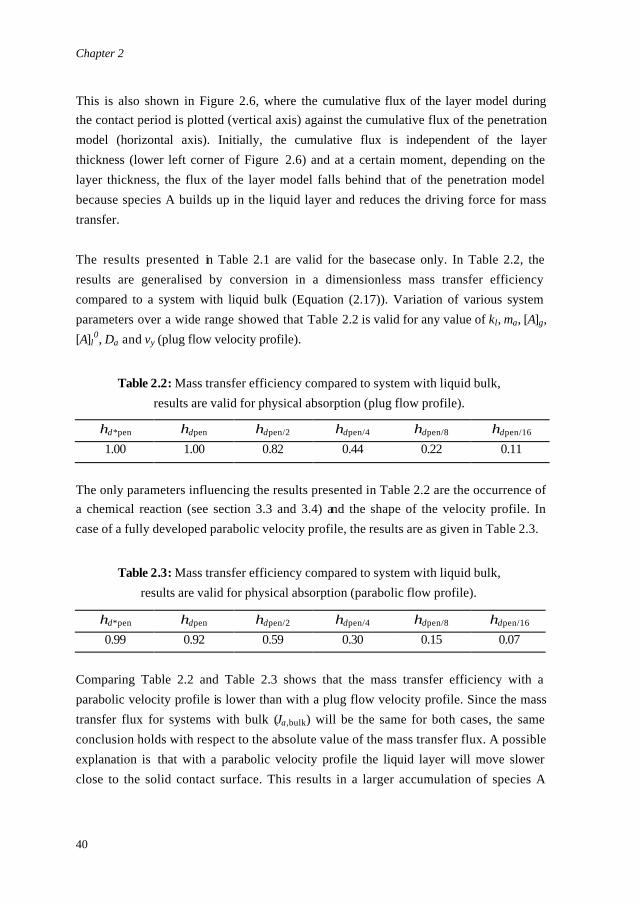
The only parameters influencing the results presented in Table 2.2 are the occurrence of a chemical reaction (see section 3.3 and 3.4) and the shape of the velocity profile. In case of a fully developed parabolic velocity profile, the results are as given in Table 2.3.

Table 2.3: Mass transfer efficiency compared to system with liquid bulk, results are valid for physical absorption (parabolic flow profile).

ηd*pen ηdpen ηdpen/2 ηdpen/4 ηdpen/8 ηdpen/16 0.99 0.92 0.59 0.30 0.15 0.07

Comparing Table 2.2 and Table 2.3 shows that the mass transfer efficiency with a parabolic velocity profile is lower than with a plug flow velocity profile. Since the mass transfer flux for systems with bulk (Ja,bulk) will be the same for both cases, the same conclusion holds with respect to the absolute value of the mass transfer flux. A possible explanation is that with a parabolic velocity profile the liquid layer will move slower close to the solid contact surface. This results in a larger accumulation of species A

Chapter 2

41

close to the solid contact surface (close to y=δ) and thus lowers the driving force and the mass transfer flux. It is found (Table 2.3) that if the layer has a thickness of at least the physical penetration

depth (δ>d*pen) the mass transfer flux approaches a maximum that corresponds to the mass transfer flux according to the penetration theory. The requirement of a layer

thickness of at least d*pen is obvious, because this is the maximum distance that species A can penetrate during the contact time. If the liquid layer has a thickness above this, species A will not at all reach the solid contact surface and the flux will not be affected by it. The fact that in case of a plug flow velocity profile the minimum required thickness

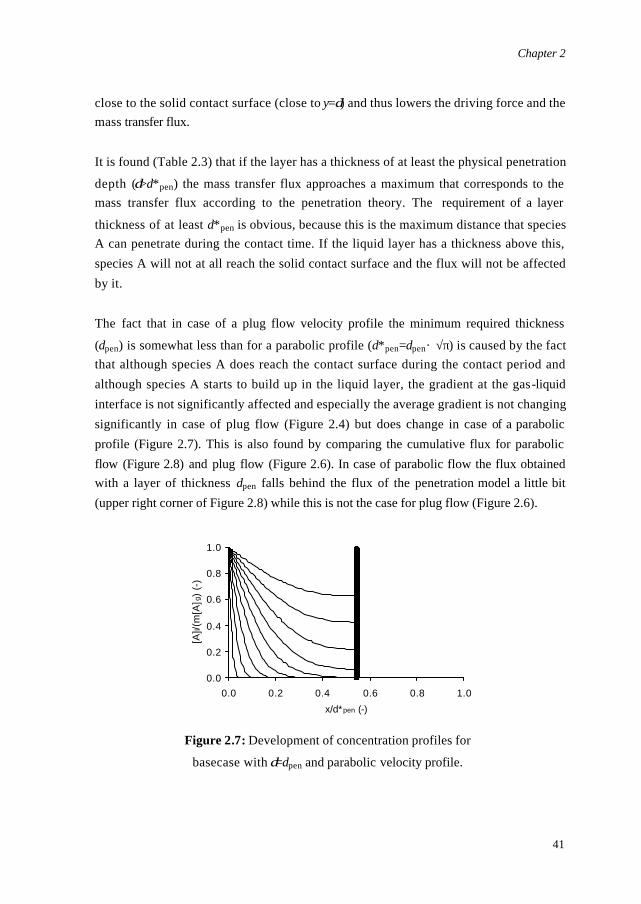
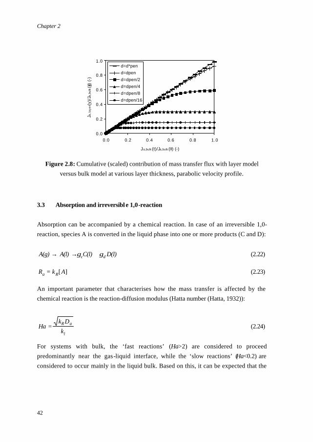
(dpen) is somewhat less than for a parabolic profile (d*pen=dpen· √π) is caused by the fact that although species A does reach the contact surface during the contact period and although species A starts to build up in the liquid layer, the gradient at the gas-liquid interface is not significantly affected and especially the average gradient is not changing significantly in case of plug flow (Figure 2.4) but does change in case of a parabolic profile (Figure 2.7). This is also found by comparing the cumulative flux for parabolic flow (Figure 2.8) and plug flow (Figure 2.6). In case of parabolic flow the flux obtained with a layer of thickness dpen falls behind the flux of the penetration model a little bit (upper right corner of Figure 2.8) while this is not the case for plug flow (Figure 2.6).

0.0

0.2

0.4

0.6

0.8

1.0

0.0 0.2 0.4 0.6 0.8 1.0

x/d*pen (-)

[A]l/

(m[A

]g)

(-)

Figure 2.7: Development of concentration profiles for

basecase with δ=dpen and parabolic velocity profile.

Chapter 2

42

0.0

0.2

0.4

0.6

0.8

1.0

0.0 0.2 0.4 0.6 0.8 1.0

Ja,bulk (t)/Ja,bulk (θ) (-)

Ja,l

ay

er(y

)/Ja

,bu

lk(

) (-

)

d=d*pen

d=dpen

d=dpen/2

d=dpen/4

d=dpen/8

d=dpen/16

Figure 2.8: Cumulative (scaled) contribution of mass transfer flux with layer model

versus bulk model at various layer thickness, parabolic velocity profile.

3.3 Absorption and irreversibl e 1,0-reaction

Absorption can be accompanied by a chemical reaction. In case of an irreversible 1,0-reaction, species A is converted in the liquid phase into one or more products (C and D):

D(l)C(l)A(l)A(g) dc γγ +→→ (2.22)

][ AkR Ra = (2.23) An important parameter that characterises how the mass transfer is affected by the chemical reaction is the reaction-diffusion modulus (Hatta number (Hatta, 1932)):

l

aR

kDk

Ha = (2.24)

For systems with bulk, the ‘fast reactions’ (Ha>2) are considered to proceed predominantly near the gas-liquid interface, while the ‘slow reactions’ (Ha<0.2) are considered to occur mainly in the liquid bulk. Based on this, it can be expected that the

Chapter 2

43

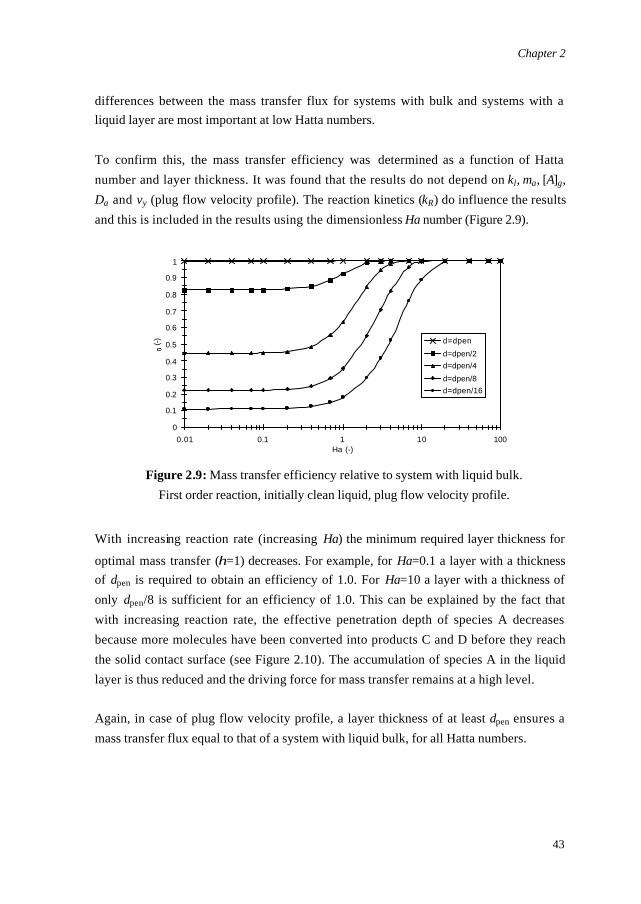
differences between the mass transfer flux for systems with bulk and systems with a liquid layer are most important at low Hatta numbers. To confirm this, the mass transfer efficiency was determined as a function of Hatta number and layer thickness. It was found that the results do not depend on kl, ma, [A]g, Da and vy (plug flow velocity profile). The reaction kinetics (kR) do influence the results and this is included in the results using the dimensionless Ha number (Figure 2.9).

0

0.1

0.2

0.3

0.4

0.5

0.6

0.7

0.8

0.9

1

0.01 0.1 1 10 100Ha (-)

(-) d=dpen

d=dpen/2

d=dpen/4

d=dpen/8

d=dpen/16

Figure 2.9: Mass transfer efficiency relative to system with liquid bulk. First order reaction, initially clean liquid, plug flow velocity profile.

With increasing reaction rate (increasing Ha) the minimum required layer thickness for

optimal mass transfer (η=1) decreases. For example, for Ha=0.1 a layer with a thickness of dpen is required to obtain an efficiency of 1.0. For Ha=10 a layer with a thickness of only dpen/8 is sufficient for an efficiency of 1.0. This can be explained by the fact that with increasing reaction rate, the effective penetration depth of species A decreases because more molecules have been converted into products C and D before they reach the solid contact surface (see Figure 2.10). The accumulation of species A in the liquid layer is thus reduced and the driving force for mass transfer remains at a high level. Again, in case of plug flow velocity profile, a layer thickness of at least dpen ensures a mass transfer flux equal to that of a system with liquid bulk, for all Hatta numbers.

Chapter 2

44

0.0

0.2

0.4

0.6

0.8

1.0

0.0 0.2 0.4 0.6 0.8 1.0

x/d (-)

[A]l/

(m[A

]g)

(-)

Figure 2.10: Development of concentration profiles for Ha=10 with δ=dpen/8.

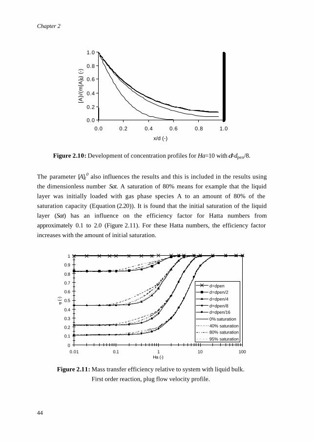
The parameter [A]l

0 also influences the results and this is included in the results using the dimensionless number Sat. A saturation of 80% means for example that the liquid layer was initially loaded with gas phase species A to an amount of 80% of the saturation capacity (Equation (2.20)). It is found that the initial saturation of the liquid layer (Sat) has an influence on the efficiency factor for Hatta numbers from approximately 0.1 to 2.0 (Figure 2.11). For these Hatta numbers, the efficiency factor increases with the amount of initial saturation.

0

0.1

0.2

0.3

0.4

0.5

0.6

0.7

0.8

0.9

1

0.01 0.1 1 10 100Ha (-)

(-)

d=dpen

d=dpen/2

d=dpen/4

d=dpen/8

d=dpen/16

0% saturation

40% saturation

80% saturation

95% saturation

Figure 2.11: Mass transfer efficiency relative to system with liquid bulk.

First order reaction, plug flow velocity profile.

Chapter 2

45

To explain this result, the three different regions have to be discussed separately. For low Hatta numbers (Ha<0.1) the mass transfer flux decreases linear with (1-Sat), this will be the same for systems with and without liquid bulk, so that the efficiency is not dependent of Sat. For high Hatta numbers (Ha>2) the reaction is so fast that the saturation decreases to zero very fast and the initial saturation (Sat) does not at all influence the flux. Again, the efficiency is not a function of Sat. In the intermediate region (0.1<Ha<2) the situation is more complex, the flux is dependent of Sat, but varies not linear with (1-Sat). In this region, the mass transfer is affected by the chemical reaction as well as the diffusion process. The diffusion process itself is however influenced by the presence of the solid contact surface. As can be seen from Figure 2.11 this becomes more important with decreasing layer thickness (the relative difference in efficiency between a saturation of 0% and 95% increases with decreasing layer thickness, see Table 2.4). This can be understood if one realises that the influence of the pre-saturation (Sat) decreases in the intermediate region with decreasing layer thickness. Thin liquid layers are saturated faster than thicker layers during the contact period. The consequence of this is that the negative influence of pre-saturation on the absorption flux is (relatively) more important with increasing layer thickness.

Table 2.4: Relative influence of initial saturation on the mass transfer efficiency as a function of layer thickness (plug flow, Ha=0.4).

dpen dpen/2 dpen/4 dpen/8 dpen/16

ηSat=0%

ηSat=95%

1.00 1.00

0.848 0.905

0.485 0.583

0.248 0.311

0.125 0.158

%0

%95

=

=

Sat

Sat

ηη

1.00

1.07

1.20

1.25

1.26

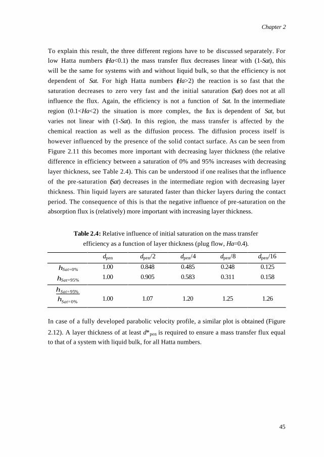
In case of a fully developed parabolic velocity profile, a similar plot is obtained (Figure

2.12). A layer thickness of at least d*pen is required to ensure a mass transfer flux equal to that of a system with liquid bulk, for all Hatta numbers.

Chapter 2

46

0

0.1

0.2

0.3

0.4

0.5

0.6

0.7

0.8

0.9

1

0.01 0.1 1 10 100

Ha (-)

(-)

d=d*pen

d=dpen

d=dpen/2

d=dpen/4

d=dpen/8

d=dpen/16

Figure 2.12: Mass transfer efficiency relative to system with liquid bulk.

First order reaction, initially clean liquid, parabolic velocity profile.

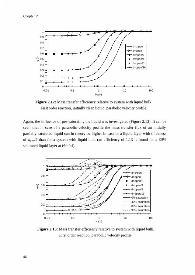
Again, the influence of pre-saturating the liquid was investigated (Figure 2.13). It can be seen that in case of a parabolic velocity profile the mass transfer flux of an initially partially saturated liquid can in theory be higher in case of a liquid layer with thickness of dpen/2 than for a system with liquid bulk (an efficiency of 1.13 is found for a 95% saturated liquid layer at Ha=0.4).

0

0.2

0.4

0.6

0.8

1

0.01 0.1 1 10 100Ha (-)

(-)

d=d*pen

d=dpen

d=dpen/2

d=dpen/4

d=dpen/8

d=dpen/16

0% saturation

40% saturation

80% saturation

95% saturation

Figure 2.13: Mass transfer efficiency relative to system with liquid bulk.

First order reaction, parabolic velocity profile.

Chapter 2

47

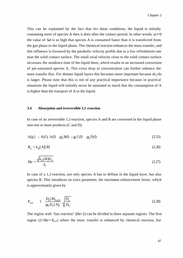
This can be explained by the fact that for these conditions, the liquid is initially containing more of species A then it does after the contact period. In other words, at t=0 the value of Sat is so high that species A is consumed faster than it is transferred from the gas phase to the liquid phase. The chemical reaction enhances the mass transfer, and this influence is favoured by the parabolic velocity profile due to a low refreshment rate near the solid contact surface. The small axial velocity close to the solid contact surface increases the residence time of the liquid there, which results in an increased conversion of pre-saturated species A. This extra drop in concentration can further enhance the mass transfer flux. For thinner liquid layers this becomes more important because dvy/dx is larger. Please note that this is not of any practical importance because in practical situations the liquid will initially never be saturated so much that the consumption of A is higher than the transport of A to the liquid. 3.4 Absorption and irreversible 1,1-reaction

In case of an irreversible 1,1-reaction, species A and B are converted in the liquid phase into one or more products (C and D):

(l)(l)(l)(l)(l(g dcb DCBA);A)A γγγ +→+→ (2.25)

]][[ BAkR Ra = (2.26)

l

aR

kDBk

Ha][

= (2.27)

In case of a 1,1-reaction, not only species A has to diffuse in the liquid layer, but also species B. This introduces an extra parameter, the maximum enhancement factor, which is approximately given by

b

a

ab

ba D

DAD

BDE

+≅∞

i

bulk

][][

1γ

(2.28)

The region with ‘fast reaction’ (Ha>2) can be divided in three separate regions. The first

region (2<Ha<<Ea∞) where the mass transfer is enhanced by chemical reaction, but

Chapter 2

48

where the supply of species B is not a limiting factor. The second region (Ha>>Ea∞) where the supply of species B is a limiting factor. The third region is the intermediate

area (Ha≈Ea∞) where a transformation from the first regime to the second regime occurs. In case of a liquid layer, there is no bulk concentration of B and the following expression was used:

b

a

ab

ba D

DAD

BDE

+≅∞

i

0

][][

1γ

(2.29)

Again the mass transfer efficiency was determined as a function of Hatta number and

layer thickness. It was found that the results depend on the value of Ea∞. It was also

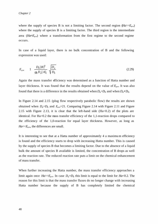
found that there is a difference in the results obtained when Da=Db and when Da≠Db. In Figure 2.14 and 2.15 (plug flow respectively parabolic flow) the results are shown

obtained when Da=Db and Ea∞=21. Comparing Figure 2.14 with Figure 2.11 and Figure 2.15 with Figure 2.13, it is clear that the left-hand side (Ha<0.2) of the plots are identical. For Ha>0.2 the mass transfer efficiency of the 1,1-reaction drops compared to the efficiency of the 1,0-reaction for equal layer thickness. However, as long as

Ha<<Ea∞, the differences are small. It is interesting to see that at a Hatta number of approximately 4 a maximu m efficiency is found and the efficiency starts to drop with increasing Hatta number. This is caused by the supply of species B that becomes a limiting factor. Due to the absence of a liquid bulk the amount of species B available is limited, the concentration of B drops as well as the reaction rate. The reduced reaction rate puts a limit on the chemical enhancement of mass transfer. When further increasing the Hatta number, the mass transfer efficiency approaches a

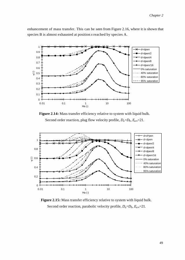
limit again once Ha>>Ea∞. In case Da=Db this limit is equal to the limit for Ha<0.2. The reason for this limit is that the mass transfer fluxes do no longer change with increasing Hatta number because the supply of B has completely limited the chemical

Chapter 2

49

enhancement of mass transfer. This can be seen from Figure 2.16, where it is shown that species B is almost exhausted at position x reached by species A.

0

0.1

0.2

0.3

0.4

0.5

0.6

0.7

0.8

0.9

1

0.01 0.1 1 10 100Ha (-)

(-)

d=dpen

d=dpen/2

d=dpen/4

d=dpen/8

d=dpen/16

0% saturation

40% saturation

80% saturation

95% saturation

Figure 2.14: Mass transfer efficiency relative to system with liquid bulk.

Second order reaction, plug flow velocity profile, Da=Db, Ea∞=21.

0

0.2

0.4

0.6

0.8

1

0.01 0.1 1 10 100Ha (-)

(-)

d=d*pen

d=dpen

d=dpen/2

d=dpen/4

d=dpen/8

d=dpen/16

0% saturation

40% saturation

80% saturation

95% saturation

Figure 2.15: Mass transfer efficiency relative to system with liquid bulk.

Second order reaction, parabolic velocity profile, Da=Db, Ea∞=21.

Chapter 2

50

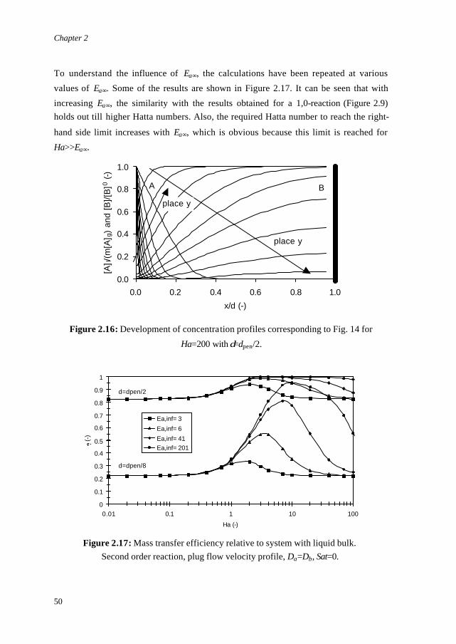
To understand the influence of Ea∞, the calculations have been repeated at various

values of Ea∞. Some of the results are shown in Figure 2.17. It can be seen that with

increasing Ea∞, the similarity with the results obtained for a 1,0-reaction (Figure 2.9) holds out till higher Hatta numbers. Also, the required Hatta number to reach the right-

hand side limit increases with Ea∞, which is obvious because this limit is reached for

Ha>>Ea∞.

0.0

0.2

0.4

0.6

0.8

1.0

0.0 0.2 0.4 0.6 0.8 1.0

x/d (-)

[A] l/

(m[A

] g)

an

d [

B]/

[B]0

(-)

place y

place y

A B

Figure 2.16: Development of concentration profiles corresponding to Fig. 14 for

Ha=200 with δ=dpen/2.

0

0.1

0.2

0.3

0.4

0.5

0.6

0.7

0.8

0.9

1

0.01 0.1 1 10 100

Ha (-)

(-)

Ea,inf= 3

Ea,inf= 6

Ea,inf= 41

Ea,inf= 201

d=dpen/2

d=dpen/8

Figure 2.17: Mass transfer efficiency relative to system with liquid bulk. Second order reaction, plug flow velocity profile, Da=Db, Sat=0.

Chapter 2

51

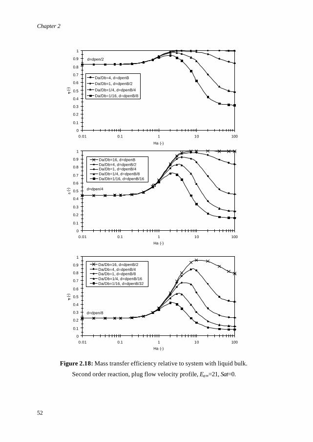
Finally, we looked at the effect of changing the ratio between Da and Db. To keep the

value of Ea∞ for the reference system with liquid bulk the same, also the concentration

of species B was adjusted, so that Ea∞ did not change. The results are shown in Figure 2.18. Again, the left-hand side of the plots is not changing and for Ha<0.2 an efficiency

of 1.0 is obtained if the condition δ≥dpen is fulfilled. In the right-hand side of the plots it can however be seen that the right limit changes with the ratio Da/Db. It can also be seen that with increasing Da/Db the plot becomes more identical with the plot of a 1,0-reaction system (Figure 2.9). This is obvious because with increasing Da/Db, the penetration depth of species B becomes smaller compared to the penetration depth of species A. In other words, with increasing Da/Db the thickness of the liquid layer becomes less limiting for species B, because in the plots the penetration depth of species

A was used as a base for the different lines. For Ha>>Ea∞ an efficiency of 1.0 is

obtained if the condition δ≥dpen,b is fulfilled (Figure 2.18).

Chapter 2

52

0

0.1

0.2

0.3

0.4

0.5

0.6

0.7

0.8

0.9

1

0.01 0.1 1 10 100

Ha (-)

(-)

Da/Db=4, d=dpenB

Da/Db=1, d=dpenB/2

Da/Db=1/4, d=dpenB/4

Da/Db=1/16, d=dpenB/8

d=dpen/2

0

0.1

0.2

0.3

0.4

0.5

0.6

0.7

0.8

0.9

1

0.01 0.1 1 10 100

Ha (-)

(-)

Da/Db=16, d=dpenBDa/Db=4, d=dpenB/2Da/Db=1, d=dpenB/4Da/Db=1/4, d=dpenB/8Da/Db=1/16, d=dpenB/16

d=dpen/4

0

0.1

0.2

0.3

0.4

0.5

0.6

0.7

0.8

0.9

1

0.01 0.1 1 10 100

Ha (-)

(-)

Da/Db=16, d=dpenB/2Da/Db=4, d=dpenB/4Da/Db=1, d=dpenB/8Da/Db=1/4, d=dpenB/16Da/Db=1/16, d=dpenB/32

d=dpen/8

Figure 2.18: Mass transfer efficiency relative to system with liquid bulk.

Second order reaction, plug flow velocity profile, Ea∞=21, Sat=0.

Chapter 2

53

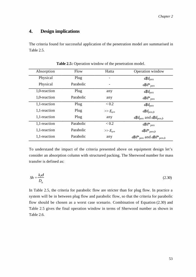
4. Design implications The criteria found for successful application of the penetration model are summarised in Table 2.5.

Table 2.5: Operation window of the penetration model.

Absorption Flow Hatta Operation window

Physical Plug - δ≥dpen Physical Parabolic - δ≥d*pen

1,0-reaction Plug any δ≥dpen 1,0-reaction Parabolic any δ≥d*pen 1,1-reaction Plug < 0.2 δ≥dpen 1,1-reaction Plug >> Ea∞ δ≥dpen,b 1,1-reaction Plug any δ≥dpen and δ≥dpen,b 1,1-reaction Parabolic < 0.2 δ≥d*pen 1,1-reaction Parabolic >> Ea∞ δ≥d*pen,b 1,1-reaction Parabolic any δ≥d*pen and δ≥d*pen,b

To understand the impact of the criteria presented above on equipment design let’s consider an absorption column with structured packing. The Sherwood number for mass transfer is defined as:

a

l

Dk

Shδ

= (2.30)

In Table 2.5, the criteria for parabolic flow are stricter than for plug flow. In practice a system will be in between plug flow and parabolic flow, so that the criteria for parabolic flow should be chosen as a worst case scenario. Combination of Equation (2.30) and Table 2.5 gives the final operation window in terms of Sherwood number as shown in Table 2.6.

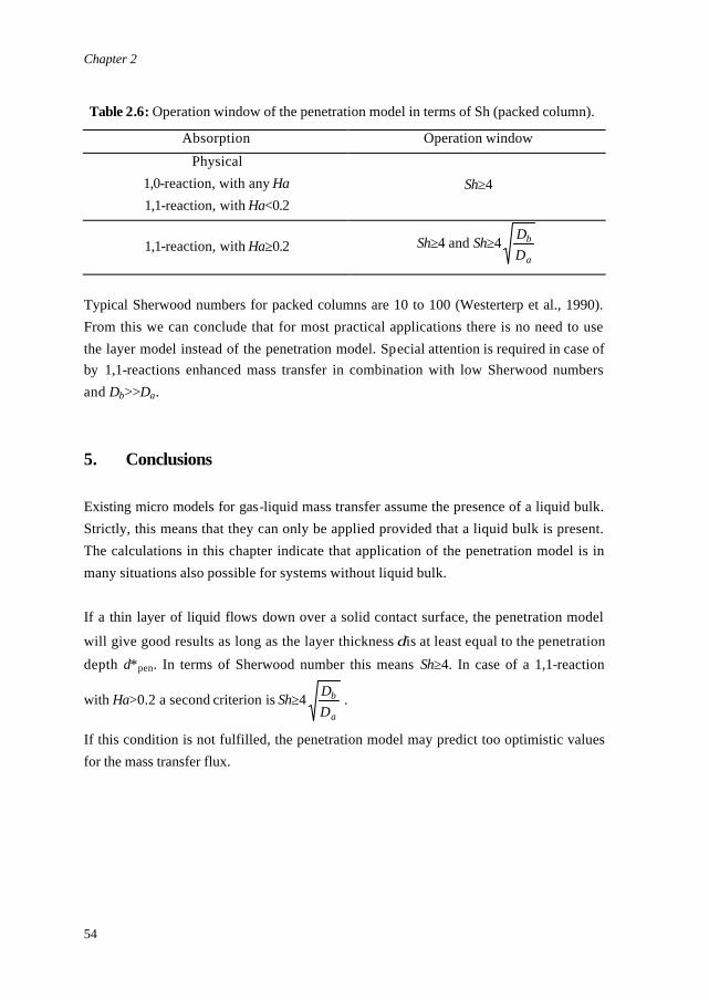
Chapter 2

54

Table 2.6: Operation window of the penetration model in terms of Sh (packed column).

Absorption Operation window

Physical 1,0-reaction, with any Ha 1,1-reaction, with Ha<0.2

Sh≥4

1,1-reaction, with Ha≥0.2 Sh≥4 and Sh≥4a

b

DD

Typical Sherwood numbers for packed columns are 10 to 100 (Westerterp et al., 1990). From this we can conclude that for most practical applications there is no need to use the layer model instead of the penetration model. Special attention is required in case of by 1,1-reactions enhanced mass transfer in combination with low Sherwood numbers and Db>>Da.

5. Conclusions Existing micro models for gas-liquid mass transfer assume the presence of a liquid bulk. Strictly, this means that they can only be applied provided that a liquid bulk is present. The calculations in this chapter indicate that application of the penetration model is in many situations also possible for systems without liquid bulk. If a thin layer of liquid flows down over a solid contact surface, the penetration model

will give good results as long as the layer thickness δ is at least equal to the penetration

depth d*pen. In terms of Sherwood number this means Sh≥4. In case of a 1,1-reaction

with Ha>0.2 a second criterion is Sh≥4a

b

DD .

If this condition is not fulfilled, the penetration model may predict too optimistic values for the mass transfer flux.

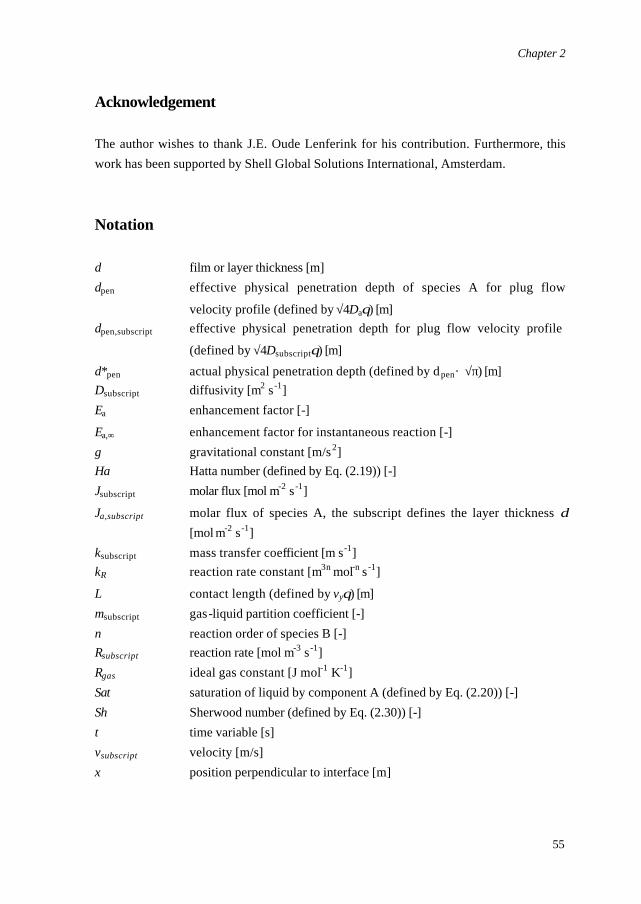
Chapter 2

55

Acknowledgement The author wishes to thank J.E. Oude Lenferink for his contribution. Furthermore, this work has been supported by Shell Global Solutions International, Amsterdam.

Notation d film or layer thickness [m] dpen effective physical penetration depth of species A for plug flow

velocity profile (defined by √4Daθ) [m] dpen,subscript effective physical penetration depth for plug flow velocity profile

(defined by √4Dsubscriptθ) [m]

d*pen actual physical penetration depth (defined by dpen· √π) [m] Dsubscript diffusivity [m2 s -1] Ea enhancement factor [-]

Ea,∞ enhancement factor for instantaneous reaction [-] g gravitational constant [m/s2] Ha Hatta number (defined by Eq. (2.19)) [-] Jsubscript molar flux [mol m-2 s -1]

Ja,subscript molar flux of species A, the subscript defines the layer thickness δ [mol m-2 s -1]

ksubscript mass transfer coefficient [m s-1] kR reaction rate constant [m3n mol-n s -1]

L contact length (defined by vyθ) [m] msubscript gas-liquid partition coefficient [-] n reaction order of species B [-] Rsubscript reaction rate [mol m-3 s -1] Rgas ideal gas constant [J mol-1 K-1] Sat saturation of liquid by component A (defined by Eq. (2.20)) [-] Sh Sherwood number (defined by Eq. (2.30)) [-] t time variable [s] vsubscript velocity [m/s] x position perpendicular to interface [m]

Chapter 2

56

X dimensionless layer thickness (defined by Eq. (2.18)) [m] y position parallel to interface [m] [] concentration [mol m-3] []subscript concentration, the subscript defines the position [mol m-3] Greek letters

δ film or layer thickness [m]

γ stoichiometric constant [-]

η efficiency compared to system with liquid bulk (relative flux) (defined by Eq. (2.17)) [-]

µ dynamic viscosity [Pa s]

θ contact time according to penetration model (defined by 4Da / πkl2) [s]

ρ density [kg m-3] Subscripts 0 initial value a,b,c,d of respectively species A, B, C or D bulk at bulk conditions g gas phase i interface i species i l liquid phase layer for systems without liquid bulk max maximum pen according to penetration theory x in x direction y in y direction

Chapter 2

57

References Danckwerts, P.V., (1951), Significance of liquid-film coefficients in gas absorption, Ind. Eng. Chem. 43, 1460-1467. Dobbins, W.E., (1956), in: McCable, M.L. and Eckenfelder, W.W. (Eds.), Biological treatment of sewage and industrial wastes, Part 2-1, Reinhold, New York. Hatta, S., (1932), Tech. Rep. Tohoku Imp. Univ. 10, 119. Higbie, R., (1935), The rate of absorption of a pure gas into a still liquid during short periods of exposure, Trans. Am. Inst. Chem. Eng. 35, 36-60. Toor, H.L. and Marchello, J.M., (1958), Film-penetration model for mass transfer and heat transfer, AIChE Journal 4, 97-101. Versteeg, G.F., Kuipers J.A.M., Beckum, F.P.H. van and Swaaij, W.P.M. van, (1989), Mass transfer with complex reversible chemical reactions – I. Single reversible chemical reaction, Chem. Eng. Sci. 44, 2295-2310. Westerterp, K.R., Swaaij, W.P.M. van and Beenackers, A.A.C.M., (1990), Chemical Reactor Design and Operation, Wiley, New York. Whitman, W.G., (1923), Preliminary experimental confirmation of the two-film theory of gas absorption, Chem. Metall. Eng. 29, 146-148.

Chapter 2

58

59

CHAPTER 3

Implementation of the penetration model in dynamic

modelling of gas-liquid processes with the presence

of a liquid bulk

3. Implementation of the penetration model in

dynamic modelling of gas-liquid processes with the

presence of a liquid bulk

Chapter 3

60

Abstract Analytical solution of models for gas-liquid reactors is restricted to a few asymptotic cases, while most numerical models make use of the physically less realistic stagnant film model. A model was developed that simulates the dynamic behaviour of gas-liquid tank reactors by simultaneously solving the Higbie penetration model for the phenomenon mass transfer accompanied by chemical reaction and the dynamic gas and liquid phase component balances. The model makes it possible to implement an alternative for the Hinterland concept1, which is usually used together with the stagnant film model. In contrast to many other numerical and analytical models the present model can be used for a wide range of conditions, the entire range of Hatta numbers, (semi-)batch reactors, multiple complex reactions and equilibrium reactions, components with different diffusion coefficients and also for systems with more than one gas phase component. By comparing the model results with analytical asymptotic solutions it was concluded that the model predicts the dynamic behaviour of the reactor satisfactorily. It is shown that under some circumstances substantial differences exist between the exact numerical and existing approximate results. It is also shown that for some special cases, differences can exist between the results obtained using the stagnant film model with Hinterland concept and the implementation of the Higbie penetration model. Experiments are required to confirm the special phenomena found in this numerical study.

1 The Hinterland concept assumes the reaction phase to consist of a stagnant film and a well-mixed bulk. Inflow and outflow of species to and from the reactor proceeds via the non-reaction phase or via the bulk of the reaction phase, but never via the stagnant film.

Chapter 3

61

1. Introduction Many chemical processes involve mass transfer of one or more gaseous components to a liquid phase in which a chemical reaction occurs. Typical examples include gas purification, oxidation, chlorination, hydrogenation (Doraiswamy et al., 1984) and hydroformylation processes. For the selection of a reactor type it is important to classify gas-liquid transfer processes on the magnitude of the reaction-diffusion modulus (Hatta number (Hatta, 1932)). The “fast reactions” (Ha>2) are considered to proceed predominantly near the gas-liquid interface, while the “slow reactions” (Ha<0.2) are considered to occur mainly in the liquid bulk. For reactions with 0.2<Ha<2, that are also frequently encountered in the chemical process industry, no distinct reaction region can be defined. In the general case the description of a gas-liquid reactor consists of the following parts: the macro model, describing the overall gas and liquid phases, and the micro model, describing the gas-liquid interphase transport of mass and/or heat in combination with the chemical reaction. Often applied, idealised, macro models are the plug flow (PFR) model and the ideal stirred tank (CISTR) model. Other possibilities include the plug flow with axial dispersion and the tanks in series model respectively (see Westerterp et al., 1990). Frequently used micro models are the stagnant film model in which mass transfer is

postulated to proceed via stationary molecular diffusion in a stagnant film of thickness δ

(Whitman, 1923), the penetration model in which the residence time θ of a fluid element at the interface is the characteristic parameter (Higbie, 1935), the surface renewal model in which a probability of replacement is introduced (Danckwerts, 1951) and the film-penetration model which is a two-parameter model combining the stagnant film and the penetration model (Dobbins, 1956 and Toor & Marchello, 1958). Solution of these micro models for mass transfer accompanied by chemical reaction analytically is restricted to cases in which many simplifying assumptions are made, e.g. reaction kinetics are simple and the rate of the reaction is either very fast or very slow

Chapter 3

62

(Sherwood et al. (1952); Danckwerts et al. (1954); Olander et al. (1960) and Huang et al. (1965)). Other authors have developed approximate analytical solutions (Krevelen et al. (1948); Onda et al. (1970); DeCoursey et al. (1982); Hikita et al. (1982)). For all other situations numerical techniques are required for solving the coupled mass balances. Overall dynamic gas-liquid reactor models can be solved in two fundamentally different ways: sequential respectively simultaneous solution of the micro and macro model. If the penetration model is used as micro model and the gas and or liquid bulk concentrations may vary significantly during the residence time of the liquid element at the mass transfer interface (e.g. the liquid bulk is not at steady state or at equilibrium), the simultaneous strategy constitutes the only correct approach. Because of its simplicity and relative ease of implementation in the overall gas-liquid reactor model (e.g. using a numerical analogy of the Hinterland concept (Westerterp et al., 1990)), the film theory is often used in numerical studies (Landau (1992); Parulekar et al. (1996)). Both these articles deal with steady state models only. Romainen and Salmi (1991) have published two papers in which a dynamic film-penetration theory is adopted. The film theory and Hinterland concept can, in many cases be applied successful. However, the penetration model and the surface renewal model are preferred since they are physically more realistic models (Westerterp et al. (1990); Versteeg et al. (1987)). Since it is not possible to implement the Hinterland analogy directly for these models, a dynamic reactor model is required that uses a somewhat different approach. Until now no such model has been published in literature. In this chapter a dynamic gas-liquid reactor model is presented which simultaneously solves the Higbie penetration model and an instationary CISTR for the gas and the liquid phase respectively. The model is suited for the phenomenon mass transfer with complex (ir)reversible chemical reaction(s) and is valid for the entire range of Hatta numbers. This chapter concentrates on describing and validating the model. A more practical application of the model for analysing the dynamics of gas-liquid processes is given in Chapter 4 and 5 of this thesis (van Elk et al. (1999)).

Chapter 3

63

2. Theory 2.1 Introduction

The problem considered is a dynamic gas-liquid reactor with mass transfer followed by an (ir)reversible chemical reaction of general order with respect to both reactants and products:

(l)(l)(l)(g) dcb DCBA γγγ ++ ←→ (3.1) with the following overall reaction rate equation:

vtsrvtsrR

qpnmqpnmRa DCBAkDCBAkR ][][][][][][][][ ,,,,,,,, −= (3.2)

The reaction rate expression is based on order-kinetics. If p,q,r and s are zero, a reversible 1,1-reaction is obtained. An irreversible 1,1-reaction is obtained by putting kR,r,s,t,v to zero. Other reactions, including multiple (in)dependent reactions, or other kinetics, like Langmuir-Hinshelwood, can easily be included in the present model. For simplicity reasons only one reaction and only one gas phase component is considered in this chapter. Also for simplicity reasons, isothermal models were assumed, the temperature can however be implemented as additional component via implementation of the energy balance. The mass transfer in the gas phase is described with the stagnant film model while for the liquid phase the penetration model is used. Further postulations in the actual dynamic reactor model are: 1. Both the gas and the liquid bulk can be assumed to be a CISTR. 2. The reaction only takes place in the liquid phase. 3. The contact time is substantially smaller than the liquid phase residence time. 2.2 Micro model

For the penetration model the balances for each species for the phenomenon mass transfer followed by a chemical reaction yields the following set of equations:

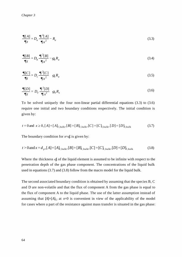
Chapter 3

64

aa RxAD

tA −=

2

2 ][][∂

∂∂

∂ (3.3)

abb RxBD

tB γ

∂∂

∂∂ −=

2

2 ][][ (3.4)

acc RxCD

tC γ

∂∂

∂∂ +=

2

2 ][][ (3.5)

add RxD

DtD

γ∂

∂∂

∂+= 2

2 ][][ (3.6)

To be solved uniquely the four non-linear partial differential equations (3.3) to (3.6) require one initial and two boundary conditions respectively. The initial condition is given by:

bulk,bulk,bulk,bulk, ][][,][][,][][,][][,0and0 llll DDCCBBAAxt ====≥= (3.7)

The boundary condition for x=δp is given by:

bulk,bulk,bulk,bulk, ][][,][][,][][,][][,and0 llllp DDCCBBAAxt =====> δ (3.8)

Where the thickness δp of the liquid element is assumed to be infinite with respect to the penetration depth of the gas phase component. The concentrations of the liquid bulk used in equations (3.7) and (3.8) follow from the macro model for the liquid bulk. The second associated boundary condition is obtained by assuming that the species B, C and D are non-volatile and that the flux of component A from the gas phase is equal to the flux of component A to the liquid phase. The use of the latter assumption instead of assuming that [A]=[A]l,i at x=0 is convenient in view of the applicability of the model for cases where a part of the resistance against mass transfer is situated in the gas phase:

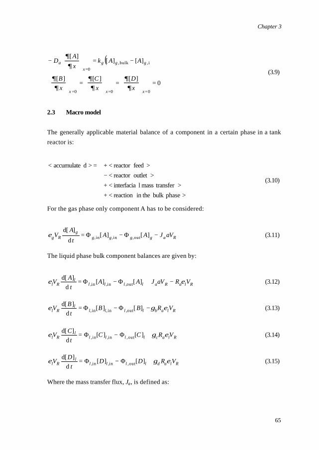
Chapter 3

65

( )

0][][][

][][][

000

i,bulk,0

=

=

=

−=

−

===

=

xxx

gggx

a

xD

xC

xB

AAkxA

D

∂∂

∂∂

∂∂

∂∂

(3.9)

2.3 Macro model

The generally applicable material balance of a component in a certain phase in a tank reactor is:

>phasebulk in thereaction < > transfermass linterfacia<

>outletreactor < >feedreactor < = >daccumulate<

++

+−

(3.10)

For the gas phase only component A has to be considered:

Raggggg

Rg aVJAAt

AV −Φ−Φ= ][][

d

]d[out,in,in,ε (3.11)

The liquid phase bulk component balances are given by:

RlaRalllll

Rl VRaVJAAt

AV εε −+Φ−Φ= ][][d

]d[out,in,in, (3.12)

Rlablllll

Rl VRBBt

BV εγε −Φ−Φ= ][][d

]d[out,in,in, (3.13)

Rlaclllll

Rl VRCCt

CV εγε +Φ−Φ= ][][d

]d[out,in,in, (3.14)

Rladlllll

Rl VRDDt

DV εγε +Φ−Φ= ][][d

]d[out,in,in, (3.15)

Where the mass transfer flux, Ja, is defined as:

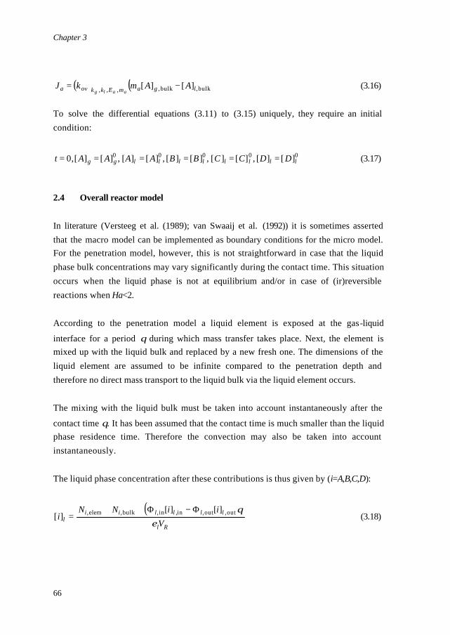
Chapter 3

66

( ) ( )bulk,bulk,,,, ][][ lgamEkkova AAmkJaalg

−= (3.16) To solve the differential equations (3.11) to (3.15) uniquely, they require an initial condition:

00000 ][][,][][,][][,][][,][][,0 llllllllgg DDCCBBAAAAt ====== (3.17) 2.4 Overall reactor model

In literature (Versteeg et al. (1989); van Swaaij et al. (1992)) it is sometimes asserted that the macro model can be implemented as boundary conditions for the micro model. For the penetration model, however, this is not straightforward in case that the liquid phase bulk concentrations may vary significantly during the contact time. This situation occurs when the liquid phase is not at equilibrium and/or in case of (ir)reversible reactions when Ha<2. According to the penetration model a liquid element is exposed at the gas-liquid

interface for a period θ during which mass transfer takes place. Next, the element is mixed up with the liquid bulk and replaced by a new fresh one. The dimensions of the liquid element are assumed to be infinite compared to the penetration depth and therefore no direct mass transport to the liquid bulk via the liquid element occurs. The mixing with the liquid bulk must be taken into account instantaneously after the

contact time θ. It has been assumed that the contact time is much smaller than the liquid phase residence time. Therefore the convection may also be taken into account instantaneously. The liquid phase concentration after these contributions is thus given by (i=A,B,C,D):

( )Rl

lllliil V

iiNNi

εθout,out,in,in,bulk,elem, ][][

][Φ−Φ++

= (3.18)

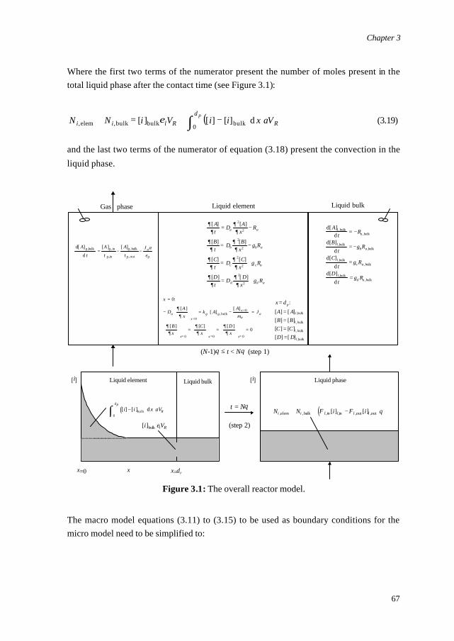
Chapter 3

67

Where the first two terms of the numerator present the number of moles present in the total liquid phase after the contact time (see Figure 3.1):

( )∫ ⋅−+=+ p

RRlii aVxiiViNNδ

ε0 bulkbulkbulk,elem, d][][][ (3.19)

and the last two terms of the numerator of equation (3.18) present the convection in the liquid phase.

∂∂

∂∂

∂∂

∂∂

γ

∂∂

∂∂

γ

∂∂

∂∂

γ

[ ] [ ]

[ ] [ ]

[ ] [ ]

[ ] [ ]

At

D Ax

R

Bt

D Bx

R

Ct

D Cx

R

Dt

D Dx

R

a a

b b a

c c a

d d a

= −

= −

= +

= +

2

2

2

2

2

2

2

2

d[ ]d

d[ ]d

d[ ]d

d[ ]d

,,

,,

,,

,,

At R

Bt

R

Ct

R

Dt

R

la

lb a

lc a

ld a

bulkbulk

bulkbulk

bulkbulk

bulkbulk

= −

= −

=

=

γ

γ

γ

x

A AB BC CD D

p

l

l

l

l

=

====

δ :

[ ] [ ][ ] [ ][ ] [ ][ ] [ ]

,

,

,

,

bulk

bulk

bulk

bulk

x

DA

xk A

A

mJ

Bx

Cx

Dx

ax

g gx

aa

x x x

=

−

= −

=

=

=

=

=

=

= = =

0

0

0

0

0 0 0

:

[ ][ ]

[ ]

[ ] [ ] [ ]

,∂

∂

∂∂

∂∂

∂∂

bulk

d[ ]

d

[ ] [ ], ,

,

,

,

A

t

A A J ag g

g

g

g

a

g

bulk in

in

bulk

out= − −

τ τ ε

( )[ ] [ ] di i x aVR

p

− ⋅∫ bulk0

δ

x=0 x x=δp

Liquid element Liquid bulk [i] Liquid phase [i]

[ ]i Vl Rbulk ε

( )N N i ii i l l l l, , , , , ,[ ] [ ]elem bulk in in out out+ + −Φ Φ θ

Liquid bulk Liquid element

(step 2)

t = Nθ

(N-1)θ ≤ t < Nθ (step 1)

Gas phase

Figure 3.1: The overall reactor model.

The macro model equations (3.11) to (3.15) to be used as boundary conditions for the micro model need to be simplified to:

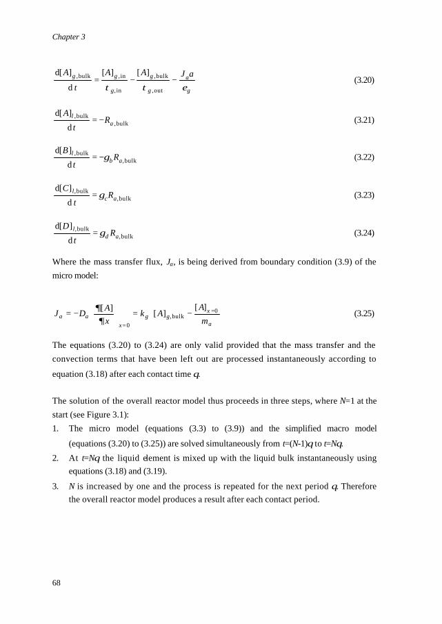
Chapter 3

68

g

a

g

g

g

gg aJAA

t

A

εττ−−=

out,

bulk,

in,

in,bulk, ][][

d

]d[ (3.20)

bulk,bulk,

d

]d[a

l Rt

A−= (3.21)

bulk,bulk,

d

]d[ab

l Rt

Bγ−= (3.22)

bulk,bulk,

d

]d[ac

l Rt

Cγ= (3.23)

bulk,bulk,

d

]d[ad

l Rt

Dγ= (3.24)

Where the mass transfer flux, Ja, is being derived from boundary condition (3.9) of the micro model:

−=

−= =

= a

xgg

xaa m

AAk

xADJ 0

bulk,0

][][][

∂∂ (3.25)

The equations (3.20) to (3.24) are only valid provided that the mass transfer and the convection terms that have been left out are processed instantaneously according to

equation (3.18) after each contact time θ. The solution of the overall reactor model thus proceeds in three steps, where N=1 at the start (see Figure 3.1): 1. The micro model (equations (3.3) to (3.9)) and the simplified macro model

(equations (3.20) to (3.25)) are solved simultaneously from t=(N-1)θ to t=Nθ.

2. At t=Nθ the liquid element is mixed up with the liquid bulk instantaneously using equations (3.18) and (3.19).

3. N is increased by one and the process is repeated for the next period θ. Therefore the overall reactor model produces a result after each contact period.

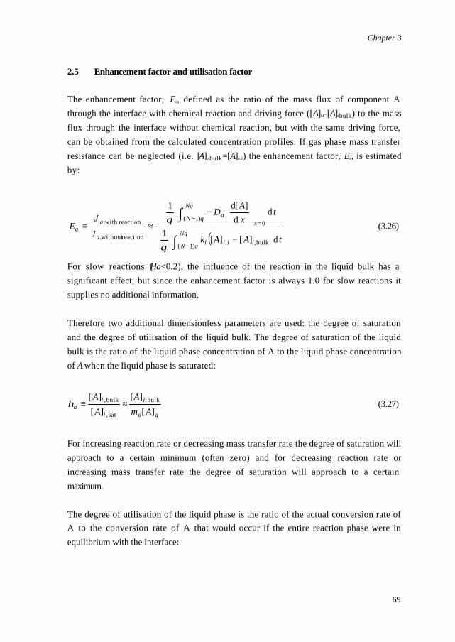
Chapter 3

69

2.5 Enhancement factor and utilisation factor

The enhancement factor, Ea, defined as the ratio of the mass flux of component A through the interface with chemical reaction and driving force ([A]l,i-[A]l,bulk) to the mass flux through the interface without chemical reaction, but with the same driving force, can be obtained from the calculated concentration profiles. If gas phase mass transfer resistance can be neglected (i.e. [A]g ,bulk=[A]g,i) the enhancement factor, Ea, is estimated by:

( )∫

∫

−

−=

−

−

≈≡θ

θ

θ

θ

θ

θN

N lll

N

Nx

a

a,

a,a

tAAk

txA

D

J

JE

)1( bulk,i,

)1(0

reactionwithout

reaction with

d][][1

dd

]d[1

(3.26)

For slow reactions (Ha<0.2), the influence of the reaction in the liquid bulk has a significant effect, but since the enhancement factor is always 1.0 for slow reactions it supplies no additional information. Therefore two additional dimensionless parameters are used: the degree of saturation and the degree of utilisation of the liquid bulk. The degree of saturation of the liquid bulk is the ratio of the liquid phase concentration of A to the liquid phase concentration of A when the liquid phase is saturated:

ga

l

l

la Am

A

A

A

][

][

][

][ bulk,

sat,

bulk, ≈≡η (3.27)

For increasing reaction rate or decreasing mass transfer rate the degree of saturation will approach to a certain minimum (often zero) and for decreasing reaction rate or increasing mass transfer rate the degree of saturation will approach to a certain maximum. The degree of utilisation of the liquid phase is the ratio of the actual conversion rate of A to the conversion rate of A that would occur if the entire reaction phase were in equilibrium with the interface:

Chapter 3

70

Rsat,)1(

)1(

V

1

laN

N

aN

N

dtR

dt

ε

ξθη θ

θ

θ

θ

∫∫

−

−≈ (3.28)

For increasing reaction rate or decreasing mass transfer rate the degree of utilisation will approach to a certain minimum (often zero) and for decreasing reaction rate or increasing mass transfer rate the degree of utilisation will approach to a certain maximum.

3. Numerical treatment In the penetration model the concentration profiles are time-dependent: they develop a solution of a system of coupled non-linear parabolic partial differential equations subject to specified initial and two point boundary conditions. The approach used to solve these models is based on the method presented by Versteeg et al. (1989), however, in the discretisation scheme two additional gridlines are introduced for the ordinary differential equations of the macro model that have to be solved simultaneously. The implicit discretisation method used is known as the Baker and Oliphant (1960) discretisation. For the time derivative a three-point backward discretisation is used (with superscript j indicating the time level) leading to (i=A,B,C,D):

tiii

ti jjj

∆+−

→−+

2][][4][3][ 11

∂∂

(3.29)

The finite difference form of the reactor model thus leads to relations between concentrations in five grid points for the micro model, four grid points for the gas phase macro model and three grid points for the liquid phase macro model, clustered as “molecules” as shown in Fig. 3.2. Only for j=0 these molecules are not possible, because no grid points with time index -1 exist. Therefore in the first step a two-point backward discretisation (Euler) is used at cost of lower order truncation error.

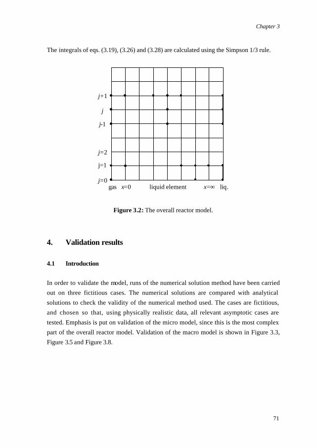
Chapter 3

71

The integrals of eqs. (3.19), (3.26) and (3.28) are calculated using the Simpson 1/3 rule.

liquid element liq.gas x=∞

j-1

j

j+1

j=2

j=1

j=0x=0

Figure 3.2: The overall reactor model.

4. Validation results 4.1 Introduction

In order to validate the model, runs of the numerical solution method have been carried out on three fictitious cases. The numerical solutions are compared with analytical solutions to check the validity of the numerical method used. The cases are fictitious, and chosen so that, using physically realistic data, all relevant asymptotic cases are tested. Emphasis is put on validation of the micro model, since this is the most complex part of the overall reactor model. Validation of the macro model is shown in Figure 3.3, Figure 3.5 and Figure 3.8.

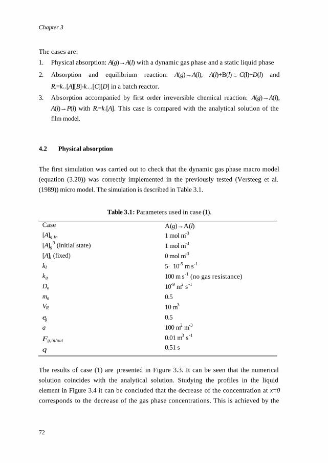
Chapter 3

72

The cases are:

1. Physical absorption: A(g)→A(l) with a dynamic gas phase and a static liquid phase

2. Absorption and equilibrium reaction: A(g)→A(l), A(l)+B(l) ←→ C(l)+D(l) and

Ra=k1,1[A][B]-k-1 ,-1[C][D] in a batch reactor.

3. Absorption accompanied by first order irreversible chemical reaction: A(g)→A(l),

A(l)→P(l) with Ra=k1[A]. This case is compared with the analytical solution of the film model.

4.2 Physical absorption

The first simulation was carried out to check that the dynamic gas phase macro model (equation (3.20)) was correctly implemented in the previously tested (Versteeg et al. (1989)) micro model. The simulation is described in Table 3.1.

Table 3.1: Parameters used in case (1).

Case [A]g,in [A]g

0 (initial state) [A]l (fixed) kl kg Da ma VR

εg a

Φg,in/out

θ

A(g)→A(l) 1 mol m-3 1 mol m-3 0 mol m-3

5· 10-5 m s-1 100 m s-1 (no gas resistance) 10-9 m2 s -1 0.5 10 m3 0.5 100 m2 m-3 0.01 m3 s -1

0.51 s

The results of case (1) are presented in Figure 3.3. It can be seen that the numerical solution coincides with the analytical solution. Studying the profiles in the liquid element in Figure 3.4 it can be concluded that the decrease of the concentration at x=0 corresponds to the decrease of the gas phase concentrations. This is achieved by the

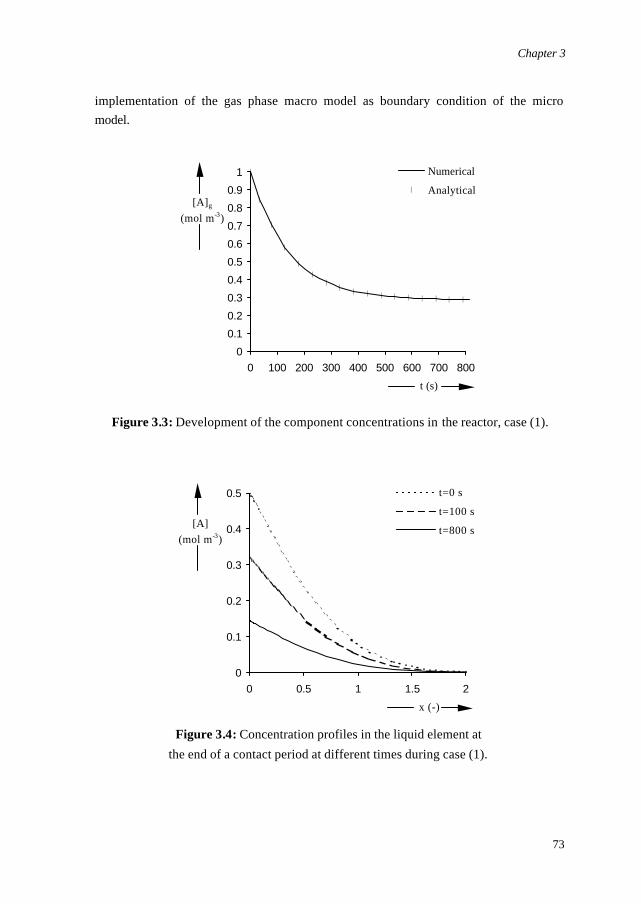
Chapter 3

73

implementation of the gas phase macro model as boundary condition of the micro model.

0

0.1

0.2

0.3

0.4

0.5

0.6

0.7

0.8

0.9

1

0 100 200 300 400 500 600 700 800

t (s)

[A]g

(mol m-3)

Numerical

Analytical

Figure 3.3: Development of the component concentrations in the reactor, case (1).

0

0.1

0.2

0.3

0.4

0.5

0 0.5 1 1.5 2

x (-)

[A](mol m-3)

t=0 s

t=100 s

t=800 s

Figure 3.4: Concentration profiles in the liquid element at

the end of a contact period at different times during case (1).

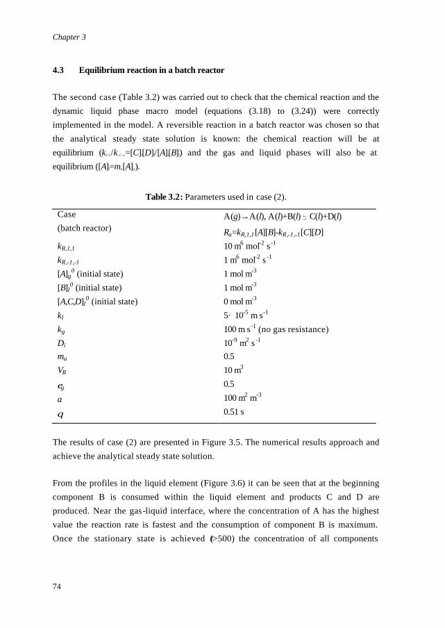
Chapter 3

74

4.3 Equilibrium reaction in a batch reactor

The second case (Table 3.2) was carried out to check that the chemical reaction and the dynamic liquid phase macro model (equations (3.18) to (3.24)) were correctly implemented in the model. A reversible reaction in a batch reactor was chosen so that the analytical steady state solution is known: the chemical reaction will be at equilibrium (k1,1/k-1 ,-1=[C]l[D]l/[A]l[B]l) and the gas and liquid phases will also be at equilibrium ([A]l=ma[A]g).

Table 3.2: Parameters used in case (2).

Case (batch reactor)

A(g)→A(l), A(l)+B(l) →← C(l)+D(l)

Ra=kR,1,1[A][B]-kR,-1,-1[C][D] kR,1,1 kR,-1,-1 [A]g

0 (initial state) [B]l

0 (initial state) [A,C,D]l

0 (initial state) kl kg Di ma VR

εg a

θ

10 m6 mol-2 s -1 1 m6 mol-2 s -1 1 mol m-3 1 mol m-3

0 mol m-3 5· 10-5 m s-1 100 m s-1 (no gas resistance) 10-9 m2 s -1 0.5 10 m3 0.5 100 m2 m-3

0.51 s

The results of case (2) are presented in Figure 3.5. The numerical results approach and achieve the analytical steady state solution. From the profiles in the liquid element (Figure 3.6) it can be seen that at the beginning component B is consumed within the liquid element and products C and D are produced. Near the gas-liquid interface, where the concentration of A has the highest value the reaction rate is fastest and the consumption of component B is maximum. Once the stationary state is achieved (t>500) the concentration of all components

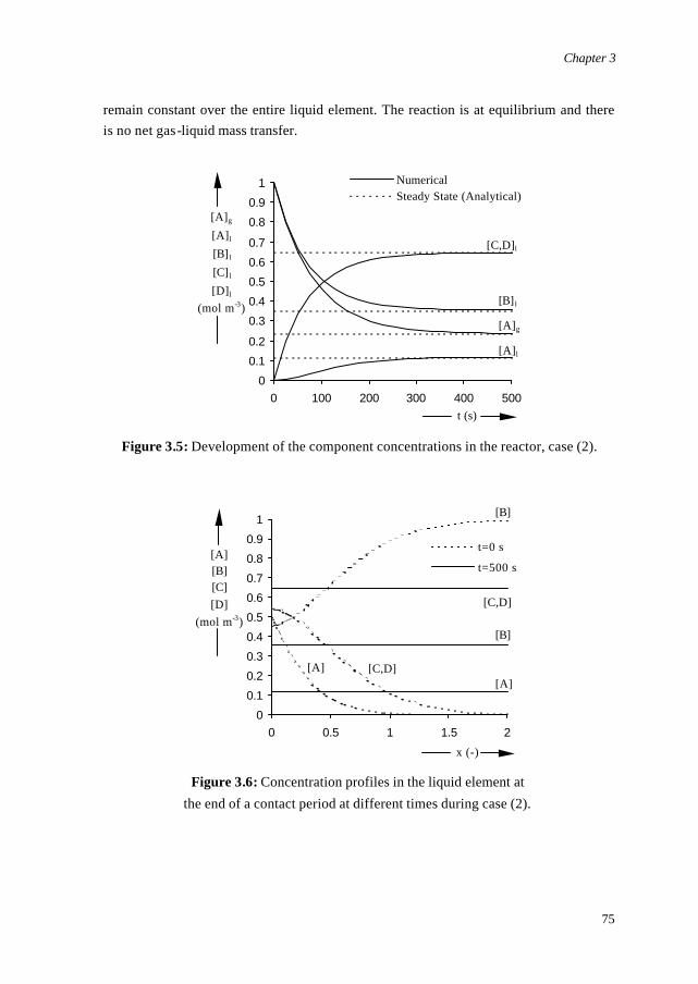
Chapter 3

75

remain constant over the entire liquid element. The reaction is at equilibrium and there is no net gas-liquid mass transfer.

0

0.1

0.2

0.3

0.4

0.5

0.6

0.7

0.8

0.9

1

0 100 200 300 400 500

t (s)

[A]g

[A]l

[B] l

[C] l

[D]l

(mol m-3)

NumericalSteady State (Analytical)

[B] l

[A]g

[A]l

[C,D]l

Figure 3.5: Development of the component concentrations in the reactor, case (2).

0

0.1

0.2

0.3

0.4

0.5

0.6

0.7

0.8

0.9

1

0 0.5 1 1.5 2

x (-)

[A][B][C][D]

(mol m-3)

t=0 s

t=500 s

[A]

[B]

[C,D]

[B]

[C,D]

[A]

Figure 3.6: Concentration profiles in the liquid element at

the end of a contact period at different times during case (2).

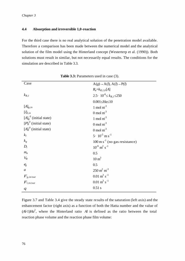
Chapter 3

76

4.4 Absorption and irreversible 1,0-reaction

For the third case there is no real analytical solution of the penetration model available. Therefore a comparison has been made between the numerical model and the analytical solution of the film model using the Hinterland concept (Westerterp et al. (1990)). Both solutions must result in similar, but not necessarily equal results. The conditions for the simulation are described in Table 3.3.

Table 3.3: Parameters used in case (3).

Case kR,1 [A]g,in [i]l,in [A]g

0 (initial state) [P]l

0 (initial state) [A]l

0 (initial state) kl kg Di ma VR

εg a

Φg,in/out

Φl,in/out

θ

A(g)→A(l), A(l)→P(l) Ra=kR,1,0[A]

2.5· 10-6≤ kR,1≤250

0.001≤Ha≤10 1 mol m-3 0 mol m-3 1 mol m-3 0 mol m-3

0 mol m-3 5· 10-5 m s-1 100 m s-1 (no gas resistance) 10-9 m2 s -1 0.5 10 m3 0.5 250 m2 m-3 0.01 m3 s -1

0.01 m3 s -1

0.51 s

Figure 3.7 and Table 3.4 give the steady state results of the saturation (left axis) and the enhancement factor (right axis) as a function of both the Hatta number and the value of (Al-1)Ha2, where the Hinterland ratio Al is defined as the ratio between the total reaction phase volume and the reaction phase film volume:

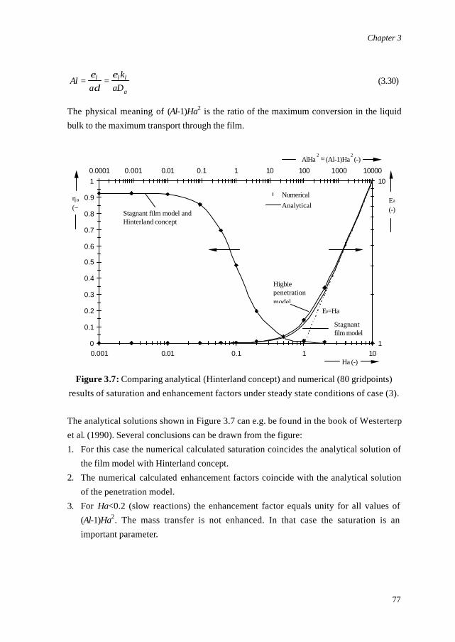
Chapter 3

77

a

lll

aDk

aAl

εδ

ε== (3.30)

The physical meaning of (Al-1)Ha2 is the ratio of the maximum conversion in the liquid bulk to the maximum transport through the film.

0

0.1

0.2

0.3

0.4

0.5

0.6

0.7

0.8

0.9

1

0.001 0.01 0.1 1 10Ha (-)

ηα

(−)

1

10

0.0001 0.001 0.01 0.1 1 10 100 1000 10000

AlHa2 ≈ (Al-1)Ha

2 (-)

Ea

(-)

NumericalAnalytical

Ea=Ha

Stagnant film model

Higbie penetration model

Stagnant film model and Hinterland concept

Figure 3.7: Comparing analytical (Hinterland concept) and numerical (80 gridpoints)

results of saturation and enhancement factors under steady state conditions of case (3). The analytical solutions shown in Figure 3.7 can e.g. be found in the book of Westerterp et al. (1990). Several conclusions can be drawn from the figure: 1. For this case the numerical calculated saturation coincides the analytical solution of

the film model with Hinterland concept. 2. The numerical calculated enhancement factors coincide with the analytical solution

of the penetration model. 3. For Ha<0.2 (slow reactions) the enhancement factor equals unity for all values of

(Al-1)Ha2. The mass transfer is not enhanced. In that case the saturation is an important parameter.

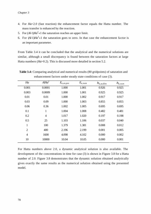
Chapter 3

78

4. For Ha>2.0 (fast reaction) the enhancement factor equals the Hatta number. The mass transfer is enhanced by the reaction.

5. For (Al-1)Ha2«1 the saturation reaches an upper limit. 6. For (Al-1)Ha2»1 the saturation goes to zero. In that case the enhancement factor is

an important parameter. From Table 3.4 it can be concluded that the analytical and the numerical solutions are similar, although a small discrepancy is found between the saturation factors at large Hatta numbers (Ha>0.2). This is discussed more detailed in section 5.2.

Table 3.4: Comparing analytical and numerical results (80 gridpoints) of saturation and enhancement factors under steady state conditions of case (3).

Ha AlHa2 Ea,an,pen Ea,num ηa,an,film ηa,num 0.001 0.003 0.01 0.03 0.06 0.1 0.2 0.5 1 2 4 10

0.0001 0.0009 0.01 0.09 0.36

1 4 25 100 400 1600 10000

1.000 1.000 1.000 1.000 1.002 1.004 1.017 1.103 1.379 2.196 4.098 10.04

1.001 1.001 1.002 1.003 1.005 1.008 1.020 1.106 1.381 2.199 4.102 10.05

0.926 0.925 0.917 0.855 0.695 0.482 0.197 0.037 0.008 0.001 0.000 0.000

0.925 0.925 0.917 0.855 0.695 0.481 0.198 0.040 0.012 0.005 0.002 0.001

For Hatta numbers above 2.0, a dynamic analytical solution is also available. The development of the concentrations in time for case (3) is shown in Figure 3.8 for a Hatta number of 2.0. Figure 3.8 demonstrates that the dynamic solution obtained analytically gives exactly the same results as the numerical solution obtained using the presented model.

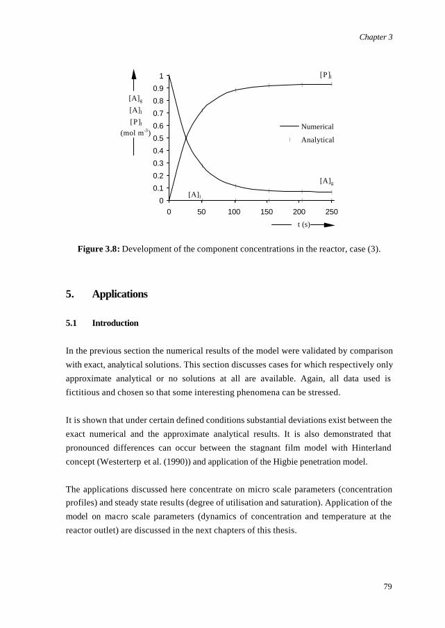
Chapter 3

79

0

0.1

0.2

0.3

0.4

0.5

0.6

0.7

0.8

0.9

1

0 50 100 150 200 250

t (s)

[A]g

[A]l

[P]l

(mol m-3)Numerical

Analytical

[P]l

[A]g

[A]l

Figure 3.8: Development of the component concentrations in the reactor, case (3).

5. Applications 5.1 Introduction

In the previous section the numerical results of the model were validated by comparison with exact, analytical solutions. This section discusses cases for which respectively only approximate analytical or no solutions at all are available. Again, all data used is fictitious and chosen so that some interesting phenomena can be stressed. It is shown that under certain defined conditions substantial deviations exist between the exact numerical and the approximate analytical results. It is also demonstrated that pronounced differences can occur between the stagnant film model with Hinterland concept (Westerterp et al. (1990)) and application of the Higbie penetration model. The applications discussed here concentrate on micro scale parameters (concentration profiles) and steady state results (degree of utilisation and saturation). Application of the model on macro scale parameters (dynamics of concentration and temperature at the reactor outlet) are discussed in the next chapters of this thesis.

Chapter 3

80

5.2 Absorption and irreversible 1,0-reaction

Additional simulations were performed for case (3), varying the specific contact area a from 2.5 m-1 till 2500 m-1. The steady state results are shown in Figure 3.9 together with the analytical solution of the stagnant film model with Hinterland concept.

0

0.1

0.2

0.3

0.4

0.5

0.6

0.7

0.8

0.9

1

0.001 0.01 0.1 1 10Ha (-)

ηα

(−)

Penetration model (numerical)Film model and Hinterland concept (analytical)

a=250 m-1

a=2500 m-1

a=25 m-1

a=2.5 m-1

Figure 3.9: Comparing analytical (Hinterland concept) and numerical results of

saturation under steady state conditions of case (3), varying the specific contact area from 2.5 m-1 to 2500 m-1.

For a specific contact area of 2.5, 25 and 250 m-1 the solution of the stagnant film model seems to coincide the solution of the penetration theory. However, at a specific higher contact areas, e.g. 2500 m-1, there is a substantial discrepancy between the solutions of both models. The penetration theory predicts substantial larger liquid phase concentrations for Hatta numbers above 0.2 than predicted by the film model with Hinterland concept. For Hatta numbers below 0.2 no discrepancy is found. The reason for this discrepancy is that the film model with Hinterland concept assumes a stagnant film, not being part of the liquid bulk, whereas the penetration model

Chapter 3

81

assumes liquid elements that are mixed up with the liquid bulk after each contact time. Therefore, the species present inside the liquid element are considered part of the liquid phase and for specific conditions this results in a larger liquid phase concentration. For processes controlled by the rate of the kinetics (Ha<0.2), these two different methods give equal results because most species are present inside the liquid bulk and the excess of species present in the liquid element (the last term of Equation (3.19)) can be neglected. For processes controlled completely or partly by the rate of the mass transfer (Ha>0.2), these two different methods give different results because the excess of species present in the liquid element (the last term of Equation (3.19)) can no longer be neglected compared to the total amount of species present in the liquid phase (Equation (3.19)). The above mentioned explanation means that the discrepancy must exist for all situations where Ha>0.2, independent of the specific contact area a. How to explain that in Figure 3.9 a discrepancy is only visible for a=2500 m-1? This is because of the scale of the y-axis in Figure 3.9. The cases for specific contact areas of 2.5, 25 and 250 m-1 have the same discrepancies between the film model with Hinterland concept and the presented implementation of the penetration theory, but the differences are not visible because of the scale of the y-axis. From Table 3.5 it is clear that there is a discrepancy for all cases once Ha>0.2.

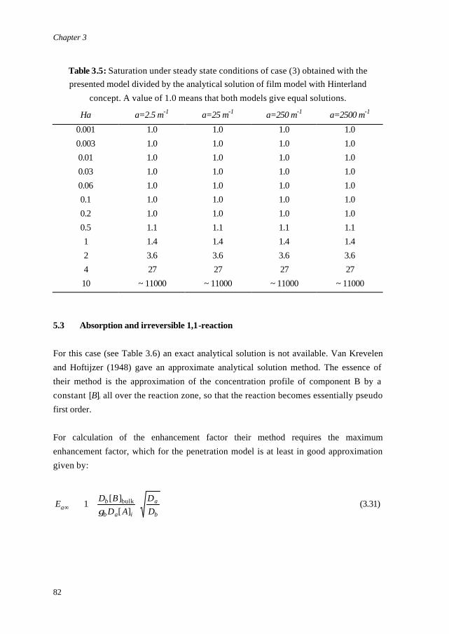
Chapter 3

82

Table 3.5: Saturation under steady state conditions of case (3) obtained with the presented model divided by the analytical solution of film model with Hinterland

concept. A value of 1.0 means that both models give equal solutions.

Ha a=2.5 m-1 a=25 m-1 a=250 m-1 a=2500 m-1

0.001 0.003 0.01 0.03 0.06 0.1 0.2 0.5 1 2 4 10

1.0 1.0 1.0 1.0 1.0 1.0 1.0 1.1 1.4 3.6 27

~ 11000

1.0 1.0 1.0 1.0 1.0 1.0 1.0 1.1 1.4 3.6 27

~ 11000

1.0 1.0 1.0 1.0 1.0 1.0 1.0 1.1 1.4 3.6 27

~ 11000

1.0 1.0 1.0 1.0 1.0 1.0 1.0 1.1 1.4 3.6 27

~ 11000 5.3 Absorption and irreversible 1,1-reaction

For this case (see Table 3.6) an exact analytical solution is not available. Van Krevelen and Hoftijzer (1948) gave an approximate analytical solution method. The essence of their method is the approximation of the concentration profile of component B by a constant [B]I all over the reaction zone, so that the reaction becomes essentially pseudo first order. For calculation of the enhancement factor their method requires the maximum enhancement factor, which for the penetration model is at least in good approximation given by:

b

a

iab

ba D

DAD

BDE

+≅∞ ][

][1 bulk

γ (3.31)

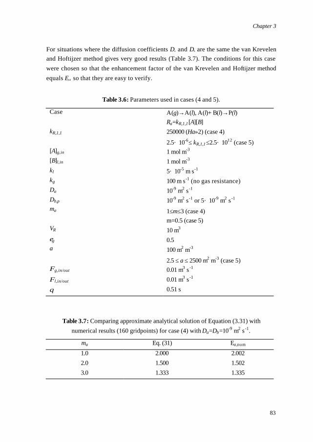
Chapter 3

83

For situations where the diffusion coefficients Da and Db are the same the van Krevelen and Hoftijzer method gives very good results (Table 3.7). The conditions for this case were chosen so that the enhancement factor of the van Krevelen and Hoftijzer method equals Ea∞ so that they are easy to verify.

Table 3.6: Parameters used in cases (4 and 5).

Case kR,1,1 [A]g,in [B]l,in kl kg Da Db,p ma VR

εg a

Φg,in/out

Φl,in/out

θ

A(g)→A(l), A(l)+ B(l)→P(l) Ra=kR,1,1[A][B] 250000 (Ha»2) (case 4)

2.5· 10-6≤ kR,1,1≤2.5· 1012 (case 5) 1 mol m-3 1 mol m-3 5· 10-5 m s-1 100 m s-1 (no gas resistance) 10-9 m2 s -1 10-9 m2 s -1 or 5· 10-9 m2 s -1

1≤m≤3 (case 4) m=0.5 (case 5) 10 m3 0.5 100 m2 m-3

2.5 ≤ a ≤ 2500 m2 m-3 (case 5) 0.01 m3 s -1

0.01 m3 s -1

0.51 s

Table 3.7: Comparing approximate analytical solution of Equation (3.31) with numerical results (160 gridpoints) for case (4) with Da=Db=10-9 m2 s -1.

ma Eq. (31) Ea,num

1.0 2.0 3.0

2.000 1.500 1.333

2.002 1.502 1.335

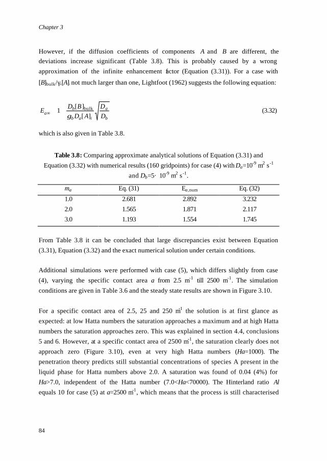
Chapter 3

84

However, if the diffusion coefficients of components A and B are different, the deviations increase significant (Table 3.8). This is probably caused by a wrong approximation of the infinite enhancement factor (Equation (3.31)). For a case with

[B]bulk/γb[A]i not much larger than one, Lightfoot (1962) suggests the following equation:

b

a

iab

ba D

DAD

BDE][

][1 bulk

γ+≅∞ (3.32)

which is also given in Table 3.8.

Table 3.8: Comparing approximate analytical solutions of Equation (3.31) and Equation (3.32) with numerical results (160 gridpoints) for case (4) with Da=10-9 m2 s -1

and Db=5· 10-9 m2 s -1.

ma Eq. (31) Ea,num Eq. (32)

1.0 2.0 3.0

2.681 1.565 1.193

2.892 1.871 1.554

3.232 2.117 1.745

From Table 3.8 it can be concluded that large discrepancies exist between Equation (3.31), Equation (3.32) and the exact numerical solution under certain conditions. Additional simulations were performed with case (5), which differs slightly from case (4), varying the specific contact area a from 2.5 m-1 till 2500 m-1. The simulation conditions are given in Table 3.6 and the steady state results are shown in Figure 3.10. For a specific contact area of 2.5, 25 and 250 m-1 the solution is at first glance as expected: at low Hatta numbers the saturation approaches a maximum and at high Hatta numbers the saturation approaches zero. This was explained in section 4.4, conclusions 5 and 6. However, at a specific contact area of 2500 m-1, the saturation clearly does not approach zero (Figure 3.10), even at very high Hatta numbers (Ha=1000). The penetration theory predicts still substantial concentrations of species A present in the liquid phase for Hatta numbers above 2.0. A saturation was found of 0.04 (4%) for Ha>7.0, independent of the Hatta number (7.0<Ha<70000). The Hinterland ratio Al equals 10 for case (5) at a=2500 m-1, which means that the process is still characterised

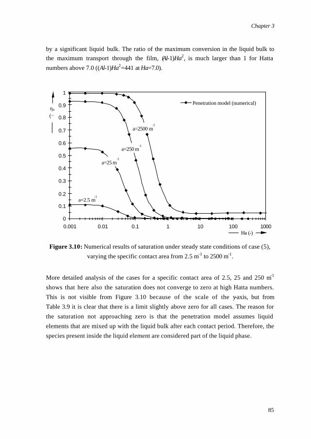
Chapter 3

85

by a significant liquid bulk. The ratio of the maximum conversion in the liquid bulk to the maximum transport through the film, (Al-1)Ha2, is much larger than 1 for Hatta numbers above 7.0 ((Al-1)Ha2=441 at Ha=7.0).

0

0.1

0.2

0.3

0.4

0.5

0.6

0.7

0.8

0.9

1

0.001 0.01 0.1 1 10 100 1000Ha (-)

ηα

(−)

Penetration model (numerical)

a=250 m-1

a=2500 m-1

a=25 m-1

a=2.5 m-1

Figure 3.10: Numerical results of saturation under steady state conditions of case (5),

varying the specific contact area from 2.5 m-1 to 2500 m-1.

More detailed analysis of the cases for a specific contact area of 2.5, 25 and 250 m-1 shows that here also the saturation does not converge to zero at high Hatta numbers. This is not visible from Figure 3.10 because of the scale of the y-axis, but from Table 3.9 it is clear that there is a limit slightly above zero for all cases. The reason for the saturation not approaching zero is that the penetration model assumes liquid elements that are mixed up with the liquid bulk after each contact period. Therefore, the species present inside the liquid element are considered part of the liquid phase.

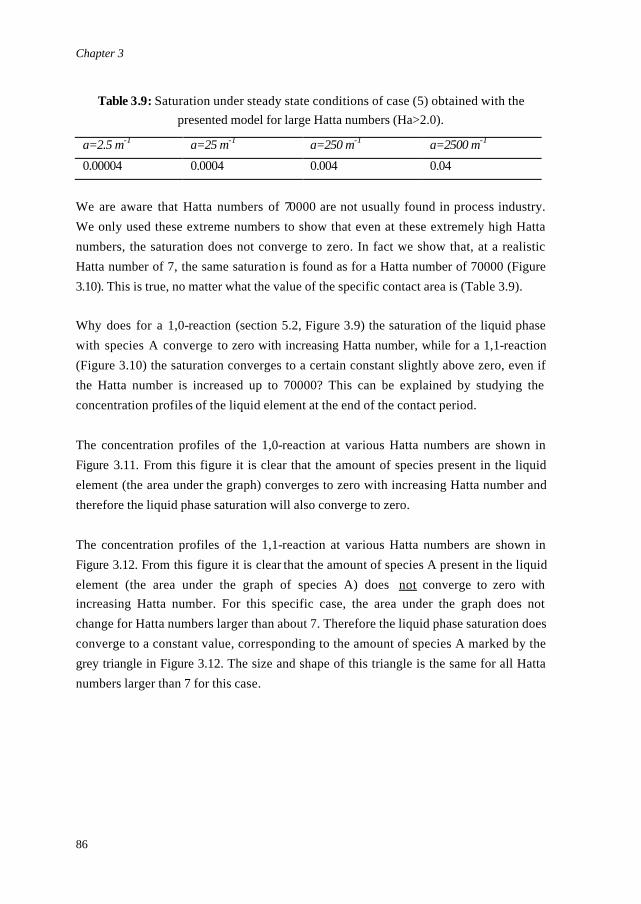
Chapter 3

86

Table 3.9: Saturation under steady state conditions of case (5) obtained with the presented model for large Hatta numbers (Ha>2.0).

a=2.5 m-1 a=25 m-1 a=250 m-1 a=2500 m-1

0.00004 0.0004 0.004 0.04

We are aware that Hatta numbers of 70000 are not usually found in process industry. We only used these extreme numbers to show that even at these extremely high Hatta numbers, the saturation does not converge to zero. In fact we show that, at a realistic Hatta number of 7, the same saturation is found as for a Hatta number of 70000 (Figure 3.10). This is true, no matter what the value of the specific contact area is (Table 3.9). Why does for a 1,0-reaction (section 5.2, Figure 3.9) the saturation of the liquid phase with species A converge to zero with increasing Hatta number, while for a 1,1-reaction (Figure 3.10) the saturation converges to a certain constant slightly above zero, even if the Hatta number is increased up to 70000? This can be explained by studying the concentration profiles of the liquid element at the end of the contact period. The concentration profiles of the 1,0-reaction at various Hatta numbers are shown in Figure 3.11. From this figure it is clear that the amount of species present in the liquid element (the area under the graph) converges to zero with increasing Hatta number and therefore the liquid phase saturation will also converge to zero. The concentration profiles of the 1,1-reaction at various Hatta numbers are shown in Figure 3.12. From this figure it is clear that the amount of species A present in the liquid element (the area under the graph of species A) does not converge to zero with increasing Hatta number. For this specific case, the area under the graph does not change for Hatta numbers larger than about 7. Therefore the liquid phase saturation does converge to a constant value, corresponding to the amount of species A marked by the grey triangle in Figure 3.12. The size and shape of this triangle is the same for all Hatta numbers larger than 7 for this case.

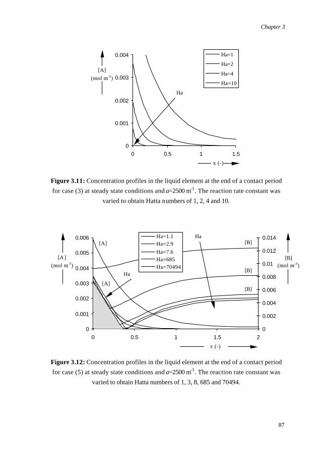
Chapter 3

87

0

0.001

0.002

0.003

0.004

0 0.5 1 1.5

x (-)

[A](mol m-3)

Ha=1

Ha=2

Ha=4

Ha=10

Ha

Figure 3.11: Concentration profiles in the liquid element at the end of a contact period for case (3) at steady state conditions and a=2500 m-1. The reaction rate constant was

varied to obtain Hatta numbers of 1, 2, 4 and 10.

0

0.001

0.002

0.003

0.004

0.005

0.006

0 0.5 1 1.5 2

x (-)

[A ](mol m-3)

0

0.002

0.004

0.006

0.008

0.01

0.012

0.014

[B](mol m-3)

Ha=1.1Ha=2.9Ha=7.6Ha=685Ha=70494

Ha

Ha[A]

[A]

[B]

[B]

[B]

Figure 3.12: Concentration profiles in the liquid element at the end of a contact period for case (5) at steady state conditions and a=2500 m-1. The reaction rate constant was

varied to obtain Hatta numbers of 1, 3, 8, 685 and 70494.

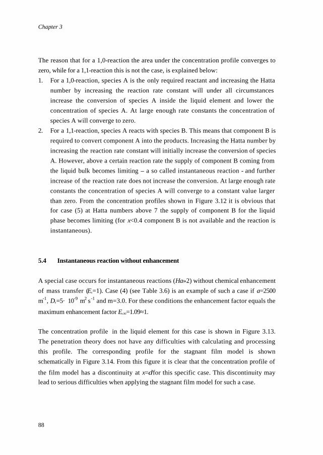
Chapter 3

88

The reason that for a 1,0-reaction the area under the concentration profile converges to zero, while for a 1,1-reaction this is not the case, is explained below: 1. For a 1,0-reaction, species A is the only required reactant and increasing the Hatta

number by increasing the reaction rate constant will under all circumstances increase the conversion of species A inside the liquid element and lower the concentration of species A. At large enough rate constants the concentration of species A will converge to zero.

2. For a 1,1-reaction, species A reacts with species B. This means that component B is required to convert component A into the products. Increasing the Hatta number by increasing the reaction rate constant will initially increase the conversion of species A. However, above a certain reaction rate the supply of component B coming from the liquid bulk becomes limiting – a so called instantaneous reaction - and further increase of the reaction rate does not increase the conversion. At large enough rate constants the concentration of species A will converge to a constant value larger than zero. From the concentration profiles shown in Figure 3.12 it is obvious that for case (5) at Hatta numbers above 7 the supply of component B for the liquid phase becomes limiting (for x<0.4 component B is not available and the reaction is instantaneous).

5.4 Instantaneous reaction without enhancement

A special case occurs for instantaneous reactions (Ha»2) without chemical enhancement of mass transfer (Ea=1). Case (4) (see Table 3.6) is an example of such a case if a=2500 m-1, Db=5· 10-9 m2 s -1 and m=3.0. For these conditions the enhancement factor equals the

maximum enhancement factor Ea∞=1.09≈1. The concentration profile in the liquid element for this case is shown in Figure 3.13. The penetration theory does not have any difficulties with calculating and processing this profile. The corresponding profile for the stagnant film model is shown schematically in Figure 3.14. From this figure it is clear that the concentration profile of

the film model has a discontinuity at x=δ for this specific case. This discontinuity may lead to serious difficulties when applying the stagnant film model for such a case.

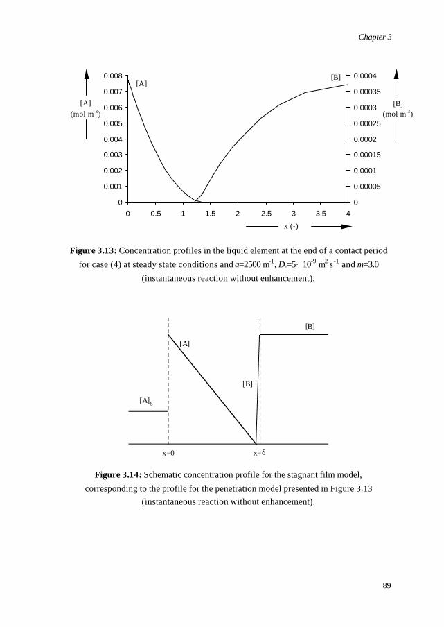
Chapter 3

89

0

0.001

0.002

0.003

0.004

0.005

0.006

0.007

0.008

0 0.5 1 1.5 2 2.5 3 3.5 4

x (-)

[A](mol m-3)

0

0.00005

0.0001

0.00015

0.0002

0.00025

0.0003

0.00035

0.0004

[B](mol m-3)

[A][B]

Figure 3.13: Concentration profiles in the liquid element at the end of a contact period for case (4) at steady state conditions and a=2500 m-1, Db=5· 10-9 m2 s -1 and m=3.0

(instantaneous reaction without enhancement).

x = δ x =0

[ B ]

[ A ]

[ B ]

[ A ] g

Figure 3.14: Schematic concentration profile for the stagnant film model, corresponding to the profile for the penetration model presented in Figure 3.13

(instantaneous reaction without enhancement).

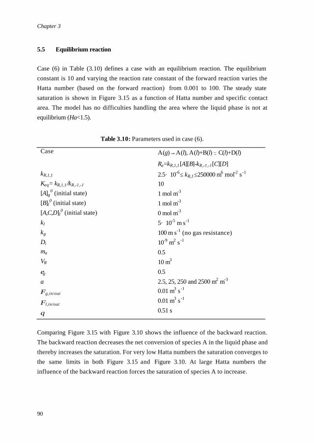
Chapter 3

90

5.5 Equilibrium reaction

Case (6) in Table (3.10) defines a case with an equilibrium reaction. The equilibrium constant is 10 and varying the reaction rate constant of the forward reaction varies the Hatta number (based on the forward reaction) from 0.001 to 100. The steady state saturation is shown in Figure 3.15 as a function of Hatta number and specific contact area. The model has no difficulties handling the area where the liquid phase is not at equilibrium (Ha<1.5).

Table 3.10: Parameters used in case (6).

Case

A(g)→A(l), A(l)+B(l) →← C(l)+D(l)

Ra=kR,1,1[A][B]-kR,-1,-1[C][D] kR,1,1 Keq= kR,1,1/kR,-1,-1 [A]g

0 (initial state) [B]l

0 (initial state) [A,C,D]l

0 (initial state) kl kg Di ma VR

εg a

Φg,in/out

Φl,in/out

θ

2.5· 10-6≤ kR,1≤250000 m6 mol-2 s -1 10 1 mol m-3 1 mol m-3

0 mol m-3 5· 10-5 m s-1 100 m s-1 (no gas resistance) 10-9 m2 s -1 0.5 10 m3 0.5 2.5, 25, 250 and 2500 m2 m-3

0.01 m3 s -1

0.01 m3 s -1

0.51 s

Comparing Figure 3.15 with Figure 3.10 shows the influence of the backward reaction. The backward reaction decreases the net conversion of species A in the liquid phase and thereby increases the saturation. For very low Hatta numbers the saturation converges to the same limits in both Figure 3.15 and Figure 3.10. At large Hatta numbers the influence of the backward reaction forces the saturation of species A to increase.

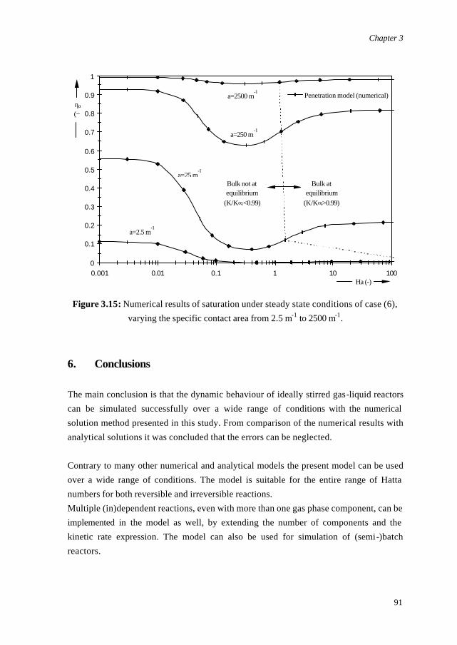
Chapter 3

91

0

0.1

0.2

0.3

0.4

0.5

0.6

0.7

0.8

0.9

1

0.001 0.01 0.1 1 10 100Ha (-)

ηα

(−)

Penetration model (numerical)

a=250 m-1

a=2500 m-1

a=25 m-1

a=2.5 m-1

Bulk atequilibrium

(K/Keq>0.99)

Bulk not atequilibrium

(K/Keq<0.99)

Figure 3.15: Numerical results of saturation under steady state conditions of case (6), varying the specific contact area from 2.5 m-1 to 2500 m-1.

6. Conclusions The main conclusion is that the dynamic behaviour of ideally stirred gas-liquid reactors can be simulated successfully over a wide range of conditions with the numerical solution method presented in this study. From comparison of the numerical results with analytical solutions it was concluded that the errors can be neglected. Contrary to many other numerical and analytical models the present model can be used over a wide range of conditions. The model is suitable for the entire range of Hatta numbers for both reversible and irreversible reactions. Multiple (in)dependent reactions, even with more than one gas phase component, can be implemented in the model as well, by extending the number of components and the kinetic rate expression. The model can also be used for simulation of (semi-)batch reactors.

Chapter 3

92

Since the Hinterland concept requires a constant mass transfer flux from the liquid film or element to the liquid bulk phase, the Hinterland concept is not directly applicable to the penetration models. The model presented in this study successfully uses a different approach to implement the simultaneous solution of the Higbie penetration and the dynamic gas-liquid macro model. Under some circumstances substantial differences exist between the exact numerical and existing approximate results. For specific cases substantial differences can exist between the results obtained using the stagnant film model with Hinterland concept and the presented implementation of the Higbie penetration model. Experiments are required to determine which model predicts the actual behaviour best. The numerical model presented in this study is especially useful for complex systems for which no analytical solutions exist and for which the stagnant film model in not accurate.

Acknowledgement This work has been supported by DSM Research, Geleen.

Notation a specific surface area [m2 m-3] A component A [-]

Al Hinterland ratio (defined by εl / δa) [-] B component B [-] C component C [-] D component D [-] Dsubscript diffusivity [m2 s -1] Esubscript enhancement factor [-]

Esubscript∞ ditto for instantaneous reaction [-] Ha Hatta number defined by (kR,m,n,p,q[A]m-1[B]n[C]p[D]qDa)0.5/kl [-]

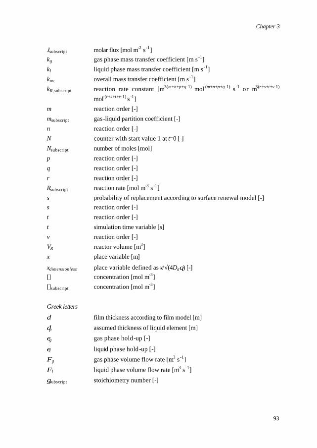
Chapter 3

93

Jsubscript molar flux [mol m-2 s -1] kg gas phase mass transfer coefficient [m s -1] kl liquid phase mass transfer coefficient [m s -1] kov overall mass transfer coefficient [m s -1] kR,subscript reaction rate constant [m3(m+n+p+q-1) mol-(m+n+p+q-1) s -1 or m3(r+s+t+v-1)

mol-(r+s+t+v-1) s -1] m reaction order [-] msubscript gas-liquid partition coefficient [-] n reaction order [-] N counter with start value 1 at t=0 [-] Nsubscript number of moles [mol] p reaction order [-] q reaction order [-] r reaction order [-] Rsubscript reaction rate [mol m-3 s -1] s probability of replacement according to surface renewal model [-] s reaction order [-] t reaction order [-] t simulation time variable [s] v reaction order [-] VR reactor volume [m3] x place variable [m]

xdimensionless place variable defined as x/√(4Daθ) [-] [] concentration [mol m-3] []subscript concentration [mol m-3] Greek letters

δ film thickness according to film model [m]

δp assumed thickness of liquid element [m]

εg gas phase hold-up [-]

εl liquid phase hold-up [-]

Φg gas phase volume flow rate [m3 s -1]

Φl liquid phase volume flow rate [m3 s -1]

γsubscript stoichiometry number [-]

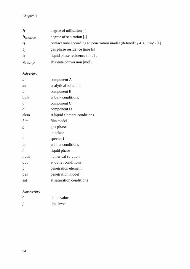
Chapter 3

94

η degree of utilisation [-]

ηsubscript degree of saturation [-]

θ contact time according to penetration model (defined by 4Da / πkl2) [s]

τg gas phase residence time [s]

τl liquid phase residence time [s]

ξsubscript absolute conversion [mol] Subscripts a component A an analytical solution b component B bulk at bulk conditions c component C d component D elem at liquid element conditions film film model g gas phase i interface i species i in at inlet conditions l liquid phase num numerical solution out at outlet conditions p penetration element pen penetration model sat at saturation conditions Superscripts 0 initial value j time level

Chapter 3

95

References Baker, G.A. and Oliphant, T.A., (1960), An implicit, numerical method for solving the two-dimensional heat equation, Quart. Appl. Math. 17, 361-373. Danckwerts, P.V., (1951), Significance of liquid-film coefficients in gas absorption, Ind. Eng. Chem. 43, 1460-1467. Danckwerts, P.V. and Kennedy, A.M., (1954), Kinetics of liquid-film process in gas absorption. Part 1: Models of the absorption process, Trans. Inst. Chem. Eng. 32, 49-53. DeCoursey, W.J., (1982), Enhancement factors for gas absorption with reversible reaction, Chem. Eng. Sci. 37, 1483-1489. Dobbins, W.E., (1956), in: McCable, M.L. and Eckenfelder, W.W. (Eds.), Biological treatment of sewage and industrial wastes, Part 2-1, Reinhold, New York. Doraiswamy, L.K. and Sharma, M.M., (1984), Heterogeneous reactions, Vol. 2, Wiley, New York. Elk, E.P. van, Borman, P.C., Kuipers, J.A.M. and Versteeg, G.F., (1999), Modelling of gas-liquid reactors – stability and dynamic behaviour of gas-liquid mass transfer accompanied by irreversible reaction, Chem. Eng. Sci. 54, 4869-4879. (Chapter 4 of this thesis). Hatta, S., (1932), Tech. Rep. Tohoku Imp. Univ., 10, 119. Higbie, R., (1935), The rate of absorption of a pure gas into a still liquid during short periods of exposure, Trans. Am. Inst. Chem. Eng. 35, 36-60. Hikita, H., Asai, S., Yano, A. and Nose, H., (1982), Kinetics of absorption of carbon dioxide into aqueous sodium sulfite solutions, AIChE Journal 28, 1009-1015. Huang, C.-J. and Kuo, C.-H., (1965), Mathematical models for mass transfer accompanied by reversible chemical reaction, AIChE Journal 11, 901-910.

Chapter 3

96

Krevelen, D.W. van and Hoftijzer, P.J., (1948), Kinetics of gas-liquid reactions. Part 1: General theory, Rec. Trav. Chim. 67, 563-568. Landau, L., (1992), Desorption with a chemical reaction, Chem. Eng. Sci. 47, 1601-1606. Leightfoot E.N., (1962), Approximate expressions for predicting the effect of fast second-order chemical reaction on interphase mass-transfer rates, Chem. Eng. Sci. 17, 1007-1011. Olander, D.R., (1960), Simultaneous mass transfer and equilibrium chemical reaction, AIChE Journal 6, 233-239. Onda, K., Sada, E., Kobayashi, T. and Fujine, M., (1970), Gas absorption accompanied with complex chemical reactions – I. Reversible chemical reactions, Chem. Eng. Sci. 25, 753-760. Parulekar, S.J. and Saidina Amin, N.A., (1996), Complex gas-liquid reactions: Feedback from bulk liquid to liquid-side film, Chem. Eng. Sci. 51, 2079-2088. Romanainen, J.J. and Salmi, T., (1991), Numerical strategies in solving gas-liquid reactor models – 1. Stagnant films and a steady state CSTR, Comput. Chem. Eng. 15, 769-781. Romanainen, J.J. and Salmi, T., (1991), Numerical strategies in solving gas-liquid reactor models – 2. Transient films and dynamic tank reactors, Comput. Chem. Eng. 15, 783-795. Sherwood, T.K. and Pigford, R.L., (1952), Absorption and extraction, p. 332, McGraw-Hill, New York. Swaaij, W.P.M. van and Versteeg, G.F., (1992), Mass transfer accompanied with complex reversible chemical reactions in gas-liquid systems: an overview, Chem. Eng. Sci. 47, 3181-3195.

Chapter 3

97

Toor, H.L. and Marchello, J.M., (1958), Film-penetration model for mass transfer and heat transfer, AIChE Journal 4, 97-101. Versteeg, G.F., Blauwhoff, P.M.M. and Swaaij, W.P.M. van, (1987), The effect of diffusivity on gas-liquid mass transfer in stirred vessels. Experiments at atmospheric and elevated pressures, Chem. Eng. Sci.42, 1103-1119. Versteeg, G.F., Kuipers J.A.M., Beckum, F.P.H. van and Swaaij, W.P.M. van, (1989), Mass transfer with complex reversible chemical reactions – I. Single reversible chemical reaction, Chem. Eng. Sci. 44, 2295-2310. Westerterp, K.R., Swaaij, W.P.M. van and Beenackers, A.A.C.M., (1990), Chemical Reactor Design and Operation, Wiley, New York. Whitman, W.G., (1923), Preliminary experimental confirmation of the two-film theory of gas absorption, Chem. Metall. Eng. 29, 146-148.

Chapter 3

98

99

CHAPTER 4

Stability and dynamic behaviour of gas-liquid mass

transfer accompanied by irreversible reaction

4. Stability and dynamic behaviour of gas-liquid

mass transfer accompanied by irreversible reaction

Chapter 4

100

Abstract The dynamic behaviour and stability of single phase reacting systems has been investigated thoroughly in the past and design rules for stable operation are available from literature. The dynamic behaviour of gas-liquid processes is considerably more complex and has received relatively little attention. General design rules for stable operation are not available. A rigorous gas-liquid reactor model is used to demonstrate the possible existence of dynamic instability (limit cycles) in gas-liquid processes. The model is also used to demonstrate that the design rules of Vleeschhouwer et al. (1992) are restricted to a specific asymptotic case. A new approximate model is presented that after implementation in bifurcation software packages can be used to obtain general applicable design rules for stable operation of ideally stirred gas-liquid reactors. The rigorous reactor model and the approximate design rules cover the whole range from kinetics controlled to mass transfer controlled systems and are powerful tools for designing gas-liquid reactors.

Chapter 4

101

1. Introduction 1.1 Single phase systems

Multiplicity, stability and dynamic behaviour of single phase reacting systems has been investigated intensively in the past. During the last 50 years a lot of papers have been devoted to this subject. Most papers (Bilous and Amundson, 1955; Aris and Amundson, 1958; Uppal et al., 1974 and 1976; Olsen and Epstein, 1993) deal with purely theoretical treatment of multiplicity and stability in single phase reactors, while other papers (Baccaro et al., 1970; Vejtasa and Schmitz, 1970; Vleeschhouwer and Fortuin, 1990; Heiszwolf and Fortuin, 1997) discuss both experimental and theoretical work. From all these papers one general and important conclusion can be drawn: whenever a system can be described sufficiently accurate by two ordinary differential equations (ODE’s) with respect to time (one heat and one material balance, like an irreversible single phase first order reaction in a CISTR reactor), the occurrence of instability is easily predicted by analysing the characteristics of the linearised system of equations for process conditions in the neighbourhood of the steady state. 1.2 Gas-liquid systems

Prediction of the dynamic behaviour of gas-liquid two phase reactors is usually more complex, since these systems involve: 1) more than two component balances, i.e. ODE’s and 2) mass transfer between the gas and the liquid phase. In literature only a few papers (Hoffman et al., 1975; Sharma et al., 1976; Huang and Varma, 1981 (two papers); Singh et al., 1982; Vleeschhouwer et al., 1992) dealt with the (dynamic) behaviour of gas-liquid processes. In none of these papers a general applicable methodology is presented to predict the dynamic behaviour of gas-liquid reactors. Huang and Varma (1981) treat the dynamic behaviour of gas-liquid reactions in non-adiabatic stirred tank reactors. Unfortunately, this paper is only applicable for the specific case of pseudo-first-order gas-liquid reactions in the so called fast reaction

Chapter 4

102

regime. For this specific case the key features of the system can be described by two ODE’s (a gas phase material and an overall heat balance) and a technique similar to that for single phase reactors can be applied to investigate the dynamic behaviour. Vleeschhouwer et al. (1992) treat the analysis of the dynamic behaviour of an industrial oxo reactor. However, this gas-liquid process is also described by only one material balance of the liquid phase component and a heat balance of the liquid phase. The gas phase components are not taken into account at all. This means that the process is simplified to a pseudo-first order single phase reacting system. This implies constant liquid phase concentrations of the gas phase components which is strictly only valid for systems with a completely saturated liquid phase (slow reaction regime and not too large Hinterland ratio’s (see Westerterp et al., 1990)). In the current chapter two new models are introduced: 1. a rigorous model that can accurately describe the dynamic behaviour of gas-liquid

reactors over a wide range of conditions. 2. an approximate model that can be used to obtain design rules for stable operation of

gas-liquid reactors. The rigorous model simultaneously solves the Higbie penetration model (partial differential equations) and the gas phase and liquid phase material balances (ODE’s) for all components. Moreover, the heat balances for both phases are taken into account on macro as well as on micro scale. The model is an improved (non-isothermal) version of the model presented and validated in Chapter 3 of this thesis (van Elk et al., 1999). Using the rigorous model it is shown that the phenomenon limit cycle (dynamic instability) found for single phase reactors can also exist in gas-liquid reactors, even if mass transfer limitations are important. Generally, these sustained oscillations have to be avoided, because they may adversely affect product quality, downstream operations, catalyst deactivation and can lead to serious difficulty in process control and to unsafe operations. It is shown that the design rules of Vleeschhouwer et al. (1992) are not generally applicable for gas-liquid reacting systems. The rigorous model has one major disadvantage: it is not suited to create a so called stability map that characterises the dynamic behaviour of the system as a function of certain selected system parameters.

Chapter 4

103

The approximate prediction is however suited to create such stability maps from which design rules can be obtained. Our approximate method is more general than the design rules presented by Huang and Varma (1981) or Vleeschhouwer et al. (1992). The rigorous model, which takes into account all relevant phenomena, is still required in order to check the approximate results for a chosen set of operating conditions.

2. Theory 2.1 Introduction

The problem considered is a dynamic gas-liquid reactor with mass transfer followed by an irreversible second order chemical reaction:

(l)(l)(l)(g) dcb DCBA γγγ +→+ (4.1)

with the following overall reaction rate equation:

]][[/1,1,0 BAekR RTE

Raact−= (4.2)

The mathematical models used are based on the following assumptions: 1. The mass transfer in the gas phase is described with the stagnant film model. 2. The mass transfer in the liquid phase is described with the penetration model. 3. The contact time according to the penetration model is small compared to the liquid

phase residence time. 4. Both the gas and the liquid phase are assumed to be perfectly mixed (i.e. CISTR’s). 5. The reaction takes place in the liquid phase only. 6. The liquid phase components (B, C and D) are non-volatile. 2.2 Rigorous model

For the penetration model the phenomenon of mass transfer accompanied by a chemical reaction is governed by the following equations for mass and heat:

Chapter 4

104

aa RxAD

tA −=

2

2 ][][∂

∂∂

∂ (4.3)

abb RxBD

tB γ

∂∂

∂∂ −=

2

2 ][][ (4.4)

( )lPl

R

lPl C

HR

x

T

Ct

T

,2

2

, ρ∂

∂

ρλ

∂

∂ ∆−−= (4.5)

To permit an unique solution of the non-linear partial differential equations (4.3) to (4.5) one initial (4.6) and two boundary conditions (4.7) and (4.8) are required:

bulk,bulk,bulk, ,][][,][][:0and0 lll TTBBAAxt ===≥= (4.6)

bulk,bulk,bulk, ,][][,][][:and0 lllp TTBBAAxt ====> δ (4.7)

( )0bulk,0

0

0bulk,

0

0][

][][

][

==

=

=

=

−=

−=

=

−=

−=

xggx

T

x

a

xgg

xaa

TThxT

J

xB

mA

AkxA

DJ

∂∂

λ

∂∂

∂∂

(4.8)

The material and energy balances describing the system on macro scale are:

g

a

g

ggg aJAA

t

A

ετ−

−= bulk,in,bulk, ][][

d

]d[ (4.9)

ggPg

T

g

ggg

CaJTT

t

T

ερτ ,

in,

d

d−

−= (4.10)

bulk,bulk,in,bulk, ][][

d]d[

al

a

l

lll RaJAA

tA

−+−

=ετ

(4.11)

Chapter 4

105

bulk,bulk,in,bulk, ][][

d]d[

abl

lll RBB

tB

γτ

−−

= (4.12)

( )lPl

R

RllPl

l

llPl

T

l

lll

CH

RVC

TTUAC

aJTT

tT

,,

cool

,

in, )(dd

ρερερτ∆−

+−

−+−

= (4.13)

The overall rigorous mathematical model (see Figure 4.1) combines the micro and macro model equations (4.3) to (4.13) by simu ltaneously solving the micro and macro model. The macro model is coupled to the micro model by the boundary conditions. The isothermal version of the model is described and validated in Chapter 3 of this thesis (van Elk et al., 1999). According to the penetration model a liquid element is exposed at the gas-liquid

interface for a period θ during which mass transfer and accompanying chemical transformation takes place. Subsequently, the element is instantaneously swept to the ideally mixed liquid bulk and replaced by a new fresh one. The dimensions of the liquid

element are assumed to be infinite compared to the penetration depth δp and therefore no direct mass and heat transport to the liquid bulk via the liquid element occurs:

bulk,bulk,in,bulk, ][][

d]d[

al

lll RAA

tA

−−

=τ

(4.14)

The liquid phase concentration directly after the element has been swept to the ideally mixed liquid bulk is:

Rl

iil V

NNi

εbulk,elem,][

+= (4.15)

The numerator represents the amount of moles present in the liquid phase after the

contact time θ (see Fig. 1):

( )∫ ⋅−+=+p

RRlii aVxiiViNNδ

ε0 bulkbulkbulk,elem, d][][][ (4.16)

For the heat balance a similar procedure is used.

Chapter 4

106

∂∂

∂∂

∂∂

∂∂

γ

∂∂

λρ

∂∂ ρ

[ ] [ ]

[ ] [ ]

, ,

At

D Ax

R

Bt

D Bx

R

Tt C

Tx

R HC

a a

b b a

l P l

R

l P l

= −

= −

= −

2

2

2

2

2

2

∆

d[ ]

d

[ ] [ ]

d[ ]

d

[ ] [ ]

, ,,

, ,,

A

t

A AR

B

t

B BR

l l l

la

l l l

lb a

bulk ,in bulkbulk

bulk ,in bulkbulk

=−

−

=−

−

τ

τγ

x

A A

B B

T T

p

l

l

l

=

=

=

=

δ :

[ ] [ ]

[ ] [ ],

,

,

bulk

bulk

bulk

d[ ]

d

[ ] [ ], , ,A

t

A A J ag g g

g

a

g

bulk in bulk=−

−τ ε

( )

x

DA

xk A

A

mJ

B

x

T

xh T T J

ax

g gx

aa

x

xg g x T

=

−

= −

=

=

−

= − =

=

=

=

==

0

0

0

0

0

00

:

[ ][ ]

[ ]

[ ]

,

,

∂

∂

∂

∂

λ∂

∂

bulk

bulk

dd

,

,

Tt

T T J aC

g g g

g

T

g P g g=

−−in

τ ρ ε dd

( ),

, ,

Tt

T T UA T TC V

R HC

l l l

l

l

l P l l R

R

l P l=

−−

−−in cool

τ ρ ε ρ∆

( )[ ] [ ] di i x aVR− ⋅∫ bulk0

x=0 x x=δp

Liquid element Liquid bulk [i] Liquid phase [i]

N N+

[ ] ε

Liquid bulk Liquid element

(step 2)

t = Nθ

(N-1)θ ≤ t < Nθ (step 1)

Gas phase

Figure 4.1: The rigorous reactor model.

2.3 Simple model (2 ODE’s) and perturbation analysis

The question arises whether or not the stability of gas-liquid reactors can be predicted without having to solve completely the complicated and time consuming rigorous reactor model presented in the previous section. This is interesting for two reasons: 1. The rigorous reactor model requires much computational efforts.

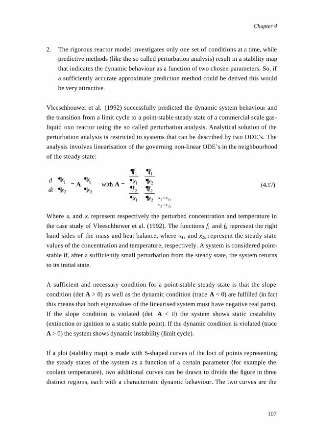
Chapter 4

107

2. The rigorous reactor model investigates only one set of conditions at a time, while predictive methods (like the so called perturbation analysis) result in a stability map that indicates the dynamic behaviour as a function of two chosen parameters. So, if a sufficiently accurate approximate prediction method could be derived this would be very attractive.

Vleeschhouwer et al. (1992) successfully predicted the dynamic system behaviour and the transition from a limit cycle to a point-stable steady state of a commercial scale gas-liquid oxo reactor using the so called perturbation analysis. Analytical solution of the perturbation analysis is restricted to systems that can be described by two ODE’s. The analysis involves linearisation of the governing non-linear ODE’s in the neighbourhood of the steady state:

s

s

xxxxx

fxf

xf

xf

x

x

x

x

dtd

22

112

2

1

2

2

1

1

1

2

1

2

1 with

=

=

=

=

∂∂

∂∂

∂∂

∂∂

∂

∂

∂

∂AA (4.17)

Where x1 and x2 represent respectively the perturbed concentration and temperature in the case study of Vleeschhower et al. (1992). The functions f1 and f2 represent the right hand sides of the mass and heat balance, where x1s and x2s represent the steady state values of the concentration and temperature, respectively. A system is considered point-stable if, after a sufficiently small perturbation from the steady state, the system returns to its initial state. A sufficient and necessary condition for a point-stable steady state is that the slope condition (det A > 0) as well as the dynamic condition (trace A < 0) are fulfilled (in fact this means that both eigenvalues of the linearised system must have negative real parts). If the slope condition is violated (det A < 0) the system shows static instability (extinction or ignition to a static stable point). If the dynamic condition is violated (trace A > 0) the system shows dynamic instability (limit cycle). If a plot (stability map) is made with S-shaped curves of the loci of points representing the steady states of the system as a function of a certain parameter (for example the coolant temperature), two additional curves can be drawn to divide the figure in three distinct regions, each with a characteristic dynamic behaviour. The two curves are the

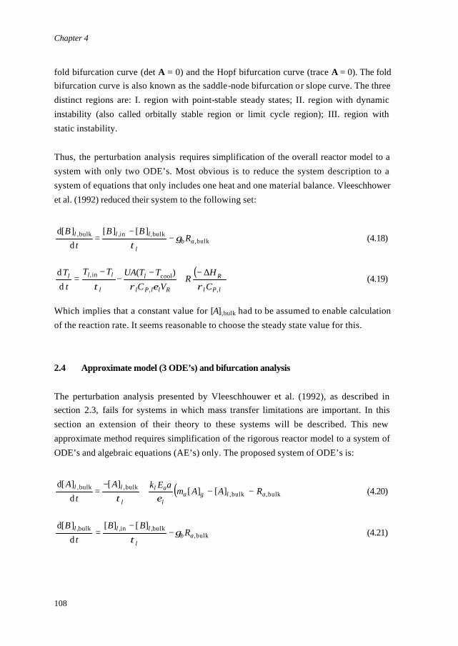
Chapter 4

108

fold bifurcation curve (det A = 0) and the Hopf bifurcation curve (trace A = 0). The fold bifurcation curve is also known as the saddle-node bifurcation or slope curve. The three distinct regions are: I. region with point-stable steady states; II. region with dynamic instability (also called orbitally stable region or limit cycle region); III. region with static instability. Thus, the perturbation analysis requires simplification of the overall reactor model to a system with only two ODE’s. Most obvious is to reduce the system description to a system of equations that only includes one heat and one material balance. Vleeschhower et al. (1992) reduced their system to the following set:

bulk,bulk,in,bulk, ][][

d]d[

abl

lll RBB

tB

γτ

−−

= (4.18)

( )lPl

R

RllPl

l

l

lll

CH

RVC

TTUATT

tT

,,

coolin, )(dd

ρερτ∆−

+−

−−

= (4.19)

Which implies that a constant value for [A]l,bulk had to be assumed to enable calculation of the reaction rate. It seems reasonable to choose the steady state value for this. 2.4 Approximate model (3 ODE’s) and bifurcation analysis

The perturbation analysis presented by Vleeschhouwer et al. (1992), as described in section 2.3, fails for systems in which mass transfer limitations are important. In this section an extension of their theory to these systems will be described. This new approximate method requires simplification of the rigorous reactor model to a system of ODE’s and algebraic equations (AE’s) only. The proposed system of ODE’s is:

( ) bulk,bulk,bulk,bulk, ][][

][d]d[

algal

al

l

ll RAAmaEkA

tA

−−+−

=ετ

(4.20)

bulk,bulk,in,bulk, ][][

d]d[

abl

lll RBB

tB

γτ

−−

= (4.21)

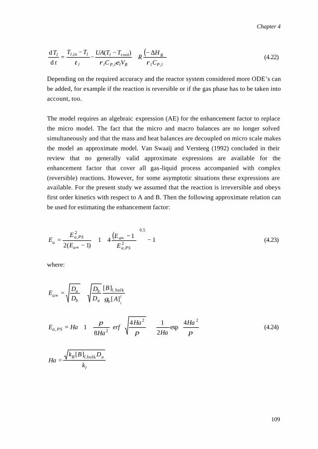
Chapter 4

109

( )lPl

R

RllPl

l

l

lll

CH

RVC

TTUATT

tT

,,

coolin, )(dd

ρερτ∆−

+−

−−

= (4.22)

Depending on the required accuracy and the reactor system considered more ODE’s can be added, for example if the reaction is reversible or if the gas phase has to be taken into account, too. The model requires an algebraic expression (AE) for the enhancement factor to replace the micro model. The fact that the micro and macro balances are no longer solved simultaneously and that the mass and heat balances are decoupled on micro scale makes the model an approximate model. Van Swaaij and Versteeg (1992) concluded in their review that no generally valid approximate expressions are available for the enhancement factor that cover all gas-liquid process accompanied with complex (reversible) reactions. However, for some asymptotic situations these expressions are available. For the present study we assumed that the reaction is irreversible and obeys first order kinetics with respect to A and B. Then the following approximate relation can be used for estimating the enhancement factor:

( )

−

−+−

= ∞

∞

1141)1(2

5.0

2,

2,

PSa

a

a

PSaa E

EE

EE (4.23)

where:

ib

l

a

b

b

aa

lA

B

DD

DDE

][

][ bulk,

γ+=∞

+

+=

πππ 22

2,4

exp2

14

81

HaHa

Haerf

HaHaE PSa (4.24)

l

alR

k

DBkHa bulk,][

=

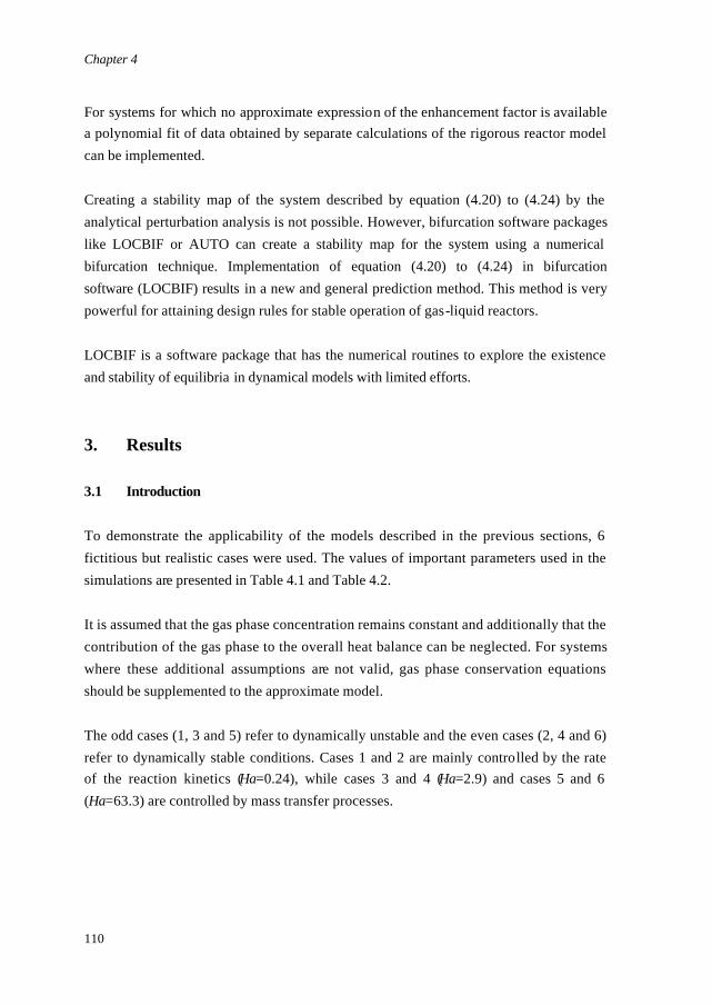
Chapter 4

110

For systems for which no approximate expression of the enhancement factor is available a polynomial fit of data obtained by separate calculations of the rigorous reactor model can be implemented. Creating a stability map of the system described by equation (4.20) to (4.24) by the analytical perturbation analysis is not possible. However, bifurcation software packages like LOCBIF or AUTO can create a stability map for the system using a numerical bifurcation technique. Implementation of equation (4.20) to (4.24) in bifurcation software (LOCBIF) results in a new and general prediction method. This method is very powerful for attaining design rules for stable operation of gas-liquid reactors. LOCBIF is a software package that has the numerical routines to explore the existence and stability of equilibria in dynamical models with limited efforts.

3. Results 3.1 Introduction

To demonstrate the applicability of the models described in the previous sections, 6 fictitious but realistic cases were used. The values of important parameters used in the simulations are presented in Table 4.1 and Table 4.2. It is assumed that the gas phase concentration remains constant and additionally that the contribution of the gas phase to the overall heat balance can be neglected. For systems where these additional assumptions are not valid, gas phase conservation equations should be supplemented to the approximate model. The odd cases (1, 3 and 5) refer to dynamically unstable and the even cases (2, 4 and 6) refer to dynamically stable conditions. Cases 1 and 2 are mainly controlled by the rate of the reaction kinetics (Ha=0.24), while cases 3 and 4 (Ha=2.9) and cases 5 and 6 (Ha=63.3) are controlled by mass transfer processes.

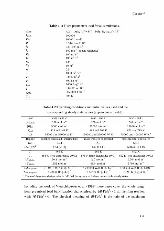
Chapter 4

111

Table 4.1: Fixed parameters used for all simulations.

Case kR0,1,1 Eact R kl kg Da Db m a VR εl a Φl

ρl CP,l λ ∆HR Tl,in

A(g)→A(l), A(l)+ B(l)→P(l) / Ra=kR,1,1[A][B] 500000 90000 J mol-1 8.314 J mol-1 K-1 3.5· 10-5 m s-1 100 m s-1 (no gas resistance) 10-9 m2 s-1 10-9 m2 s-1 1.0 10 m3 0.5 1000 m2 m-3 0.005 m3 s-1

800 kg m-3 2000 J kg-1 K-1 0.02 W m-1 K-1 -160000 J mol-1 303 K

Table 4.2:Operating conditions and initial values used and the corresponding steady state values (approximate model).

Case case 1 and 2 case 3 and 4 case 5 and 6 [A]g,bulk [B]l,in Tcool UA

100 mol m-3 5000 mol m-3

425 and 441 K 35000 and 55000 W K-1

100 mol m-3 25000 mol m-3

469 and 507 K 150000 and 250000 W K-1

5.0 mol m-3 25000 mol m-3

673 and 715 K 75000 and 100000 W K-1

Regime Has

(Al-1)Ha2

kinetics controlled / intermediate 0.24

0.94 (≈1.0)

mass transfer controlled 2.9

140 (>1.0)

mass transfer controlled 63.3

66074 (>>1.0)

Ts T0

[A]l,bulk,s [B]l,bulk,s

468 K 488 K (step disturbance 20°C)

50.1 mol m-3 1558 mol m-3

565 K 575 K (step disturbance 10°C)

2.0 mol m-3 4354 mol m-3

842 K 852 K (step disturbance 10°C)

0.004 mol m-3 3760 mol m-3

UAdesign rule

Tcool design rule > 50418 W/K (Fig. 4.5) *

> 438 K (Fig. 4.5) * > 214848 W/K (Fig. 4.7) *

> 509 K (Fig. 4.7) * > 98934 W/K (Fig. 4.10) *

> 693 K (Fig. 4.10) * * If one of these two design rules is fulfilled the system will show point stable steady states.

Including the work of Vleeschhouwer et al. (1992) these cases cover the whole range from pre-mixed feed bulk reaction characterised by (Al-1)Ha2<<1 till fast film reaction with (Al-1)Ha2>>1. The physical meaning of (Al-1)Ha2 is the ratio of the maximum

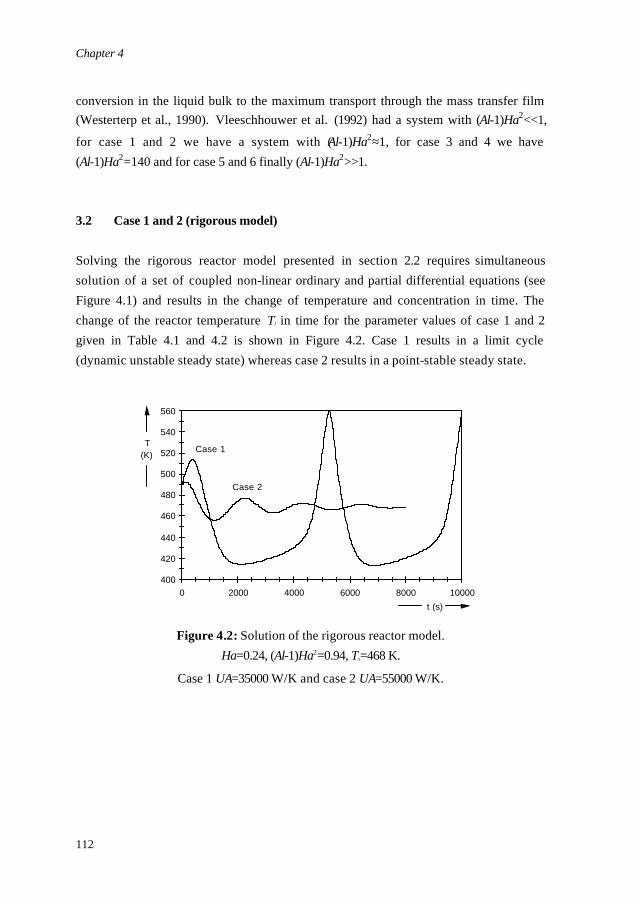
Chapter 4

112

conversion in the liquid bulk to the maximum transport through the mass transfer film (Westerterp et al., 1990). Vleeschhouwer et al. (1992) had a system with (Al-1)Ha2<<1,

for case 1 and 2 we have a system with (Al-1)Ha2≈1, for case 3 and 4 we have (Al-1)Ha2=140 and for case 5 and 6 finally (Al-1)Ha2>>1. 3.2 Case 1 and 2 (rigorous model)

Solving the rigorous reactor model presented in section 2.2 requires simultaneous solution of a set of coupled non-linear ordinary and partial differential equations (see Figure 4.1) and results in the change of temperature and concentration in time. The change of the reactor temperature Tl in time for the parameter values of case 1 and 2 given in Table 4.1 and 4.2 is shown in Figure 4.2. Case 1 results in a limit cycle (dynamic unstable steady state) whereas case 2 results in a point-stable steady state.

400

420

440

460

480

500

520

540

560

0 2000 4000 6000 8000 10000

t (s)

T(K)

Case 1

Case 2

Figure 4.2: Solution of the rigorous reactor model. Ha=0.24, (Al-1)Ha2=0.94, Ts=468 K.

Case 1 UA=35000 W/K and case 2 UA=55000 W/K.

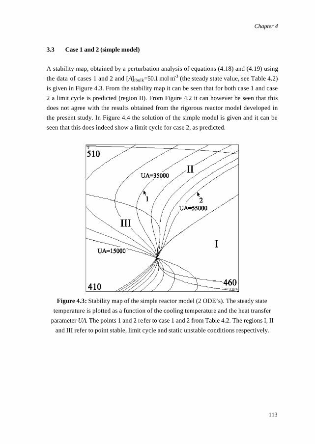
Chapter 4

113

3.3 Case 1 and 2 (simple model)

A stability map, obtained by a perturbation analysis of equations (4.18) and (4.19) using the data of cases 1 and 2 and [A]l,bulk=50.1 mol m-3 (the steady state value, see Table 4.2) is given in Figure 4.3. From the stability map it can be seen that for both case 1 and case 2 a limit cycle is predicted (region II). From Figure 4.2 it can however be seen that this does not agree with the results obtained from the rigorous reactor model developed in the present study. In Figure 4.4 the solution of the simple model is given and it can be seen that this does indeed show a limit cycle for case 2, as predicted.

Figure 4.3: Stability map of the simple reactor model (2 ODE’s). The steady state temperature is plotted as a function of the cooling temperature and the heat transfer

parameter UA. The points 1 and 2 refer to case 1 and 2 from Table 4.2. The regions I, II and III refer to point stable, limit cycle and static unstable conditions respectively.

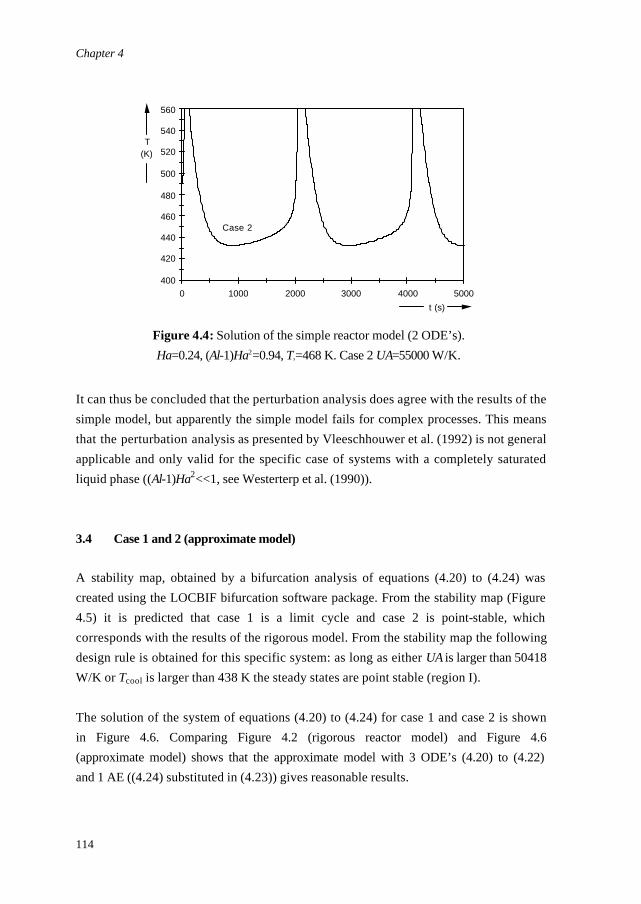
Chapter 4

114

400

420

440

460

480

500

520

540

560

0 1000 2000 3000 4000 5000

t (s)

T(K)

Case 2

Figure 4.4: Solution of the simple reactor model (2 ODE’s). Ha=0.24, (Al-1)Ha2=0.94, Ts=468 K. Case 2 UA=55000 W/K.

It can thus be concluded that the perturbation analysis does agree with the results of the simple model, but apparently the simple model fails for complex processes. This means that the perturbation analysis as presented by Vleeschhouwer et al. (1992) is not general applicable and only valid for the specific case of systems with a completely saturated liquid phase ((Al-1)Ha2<<1, see Westerterp et al. (1990)). 3.4 Case 1 and 2 (approximate model)

A stability map, obtained by a bifurcation analysis of equations (4.20) to (4.24) was created using the LOCBIF bifurcation software package. From the stability map (Figure 4.5) it is predicted that case 1 is a limit cycle and case 2 is point-stable, which corresponds with the results of the rigorous model. From the stability map the following design rule is obtained for this specific system: as long as either UA is larger than 50418 W/K or Tcool is larger than 438 K the steady states are point stable (region I). The solution of the system of equations (4.20) to (4.24) for case 1 and case 2 is shown in Figure 4.6. Comparing Figure 4.2 (rigorous reactor model) and Figure 4.6 (approximate model) shows that the approximate model with 3 ODE’s (4.20) to (4.22) and 1 AE ((4.24) substituted in (4.23)) gives reasonable results.

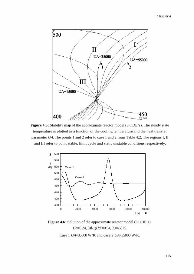
Chapter 4

115

Figure 4.5: Stability map of the approximate reactor model (3 ODE’s). The steady state

temperature is plotted as a function of the cooling temperature and the heat transfer parameter UA. The points 1 and 2 refer to case 1 and 2 from Table 4.2. The regions I, II

and III refer to point stable, limit cycle and static unstable conditions respectively.

400

420

440

460

480

500

520

540

560

0 2000 4000 6000 8000 10000

t (s)

T(K) Case 1

Case 2

Figure 4.6: Solution of the approximate reactor model (3 ODE’s). Ha=0.24, (Al-1)Ha2=0.94, Ts=468 K.

Case 1 UA=35000 W/K and case 2 UA=55000 W/K.

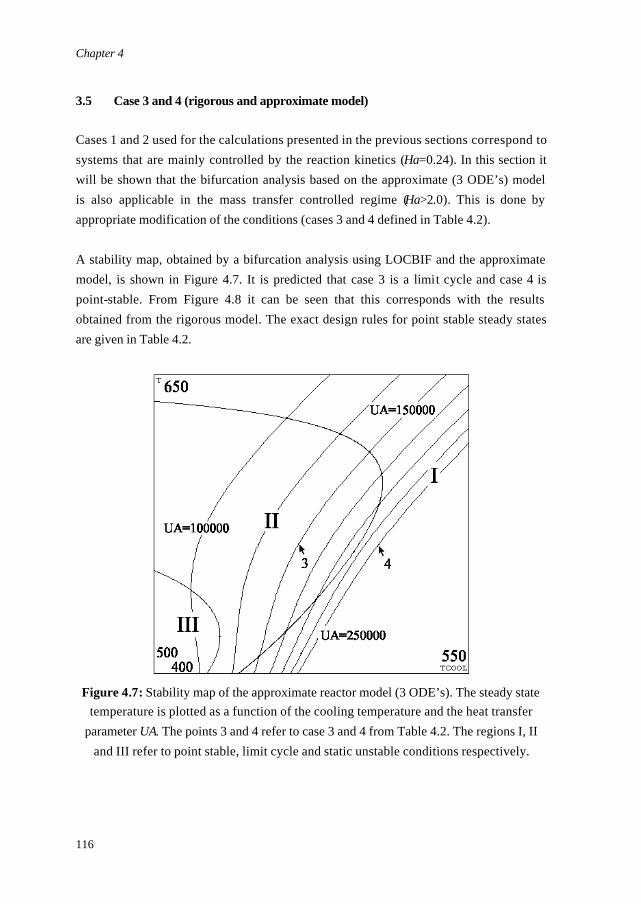
Chapter 4

116

3.5 Case 3 and 4 (rigorous and approximate model)

Cases 1 and 2 used for the calculations presented in the previous sections correspond to systems that are mainly controlled by the reaction kinetics (Ha=0.24). In this section it will be shown that the bifurcation analysis based on the approximate (3 ODE’s) model is also applicable in the mass transfer controlled regime (Ha>2.0). This is done by appropriate modification of the conditions (cases 3 and 4 defined in Table 4.2). A stability map, obtained by a bifurcation analysis using LOCBIF and the approximate model, is shown in Figure 4.7. It is predicted that case 3 is a limit cycle and case 4 is point-stable. From Figure 4.8 it can be seen that this corresponds with the results obtained from the rigorous model. The exact design rules for point stable steady states are given in Table 4.2.

Figure 4.7: Stability map of the approximate reactor model (3 ODE’s). The steady state temperature is plotted as a function of the cooling temperature and the heat transfer

parameter UA. The points 3 and 4 refer to case 3 and 4 from Table 4.2. The regions I, II and III refer to point stable, limit cycle and static unstable conditions respectively.

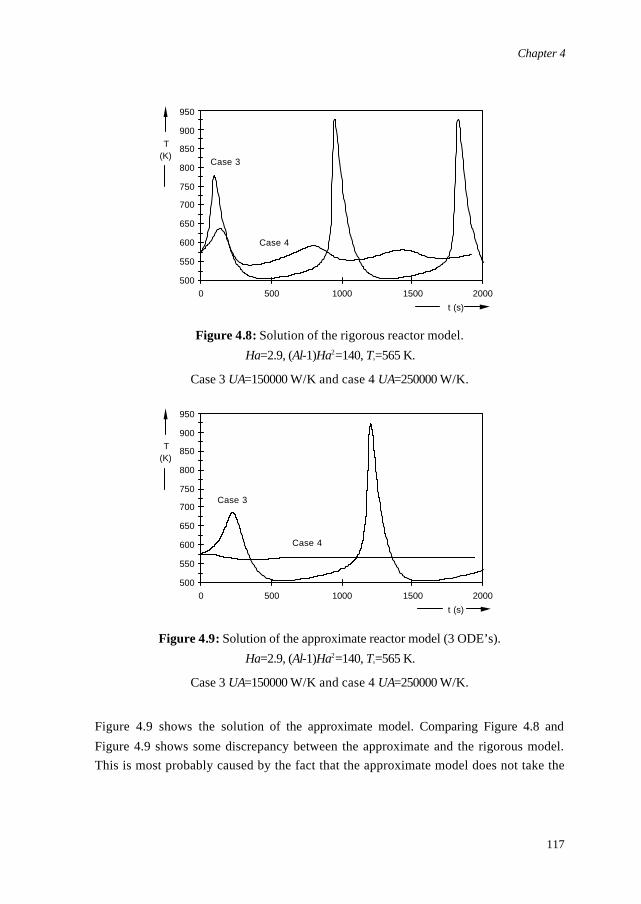
Chapter 4

117

500

550

600

650

700

750

800

850

900

950

0 500 1000 1500 2000

t (s)

T(K)

Case 3

Case 4

Figure 4.8: Solution of the rigorous reactor model.

Ha=2.9, (Al-1)Ha2=140, Ts=565 K.

Case 3 UA=150000 W/K and case 4 UA=250000 W/K.

500

550

600

650

700

750

800

850

900

950

0 500 1000 1500 2000

t (s)

T(K)

Case 3

Case 4

Figure 4.9: Solution of the approximate reactor model (3 ODE’s). Ha=2.9, (Al-1)Ha2=140, Ts=565 K.

Case 3 UA=150000 W/K and case 4 UA=250000 W/K.

Figure 4.9 shows the solution of the approximate model. Comparing Figure 4.8 and Figure 4.9 shows some discrepancy between the approximate and the rigorous model. This is most probably caused by the fact that the approximate model does not take the

Chapter 4

118

temperature profile on micro scale into account (Vas Bhat et al., 1997). Moreover, for these cases the heat of reaction in produced mainly in the mass transfer film near the gas-liquid interface, contrary to the approximate rigorous method which assumes bulk heat generation. 3.6 Case 5 and 6 (rigorous and approximate model)

Cases 3 and 4 are mainly controlled by mass transfer (Ha=2.9, (Al-1)Ha2=140), but the concentration of the gas phase component A in the liquid bulk is not yet completely zero ([A]l,bulk=2.0 mol m-3). Cases 5 and 6 are characterised by a very fast reaction (Ha=63.3, (Al-1)Ha2>>1), so that the liquid bulk is fully depleted ([A]l,bulk=0.004 mol m-3). This is achieved by appropriate modification of the conditions (Table 4.2).

Figure 4.10: Stability map of the approximate reactor model (3 ODE’s). The steady

state temperature is plotted as a function of the cooling temperature and the heat transfer parameter UA. The points 5 and 6 refer to case 5 and 6 from Table 4.2. The regions I, II

and III refer to point stable, limit cycle and static unstable conditions respectively.

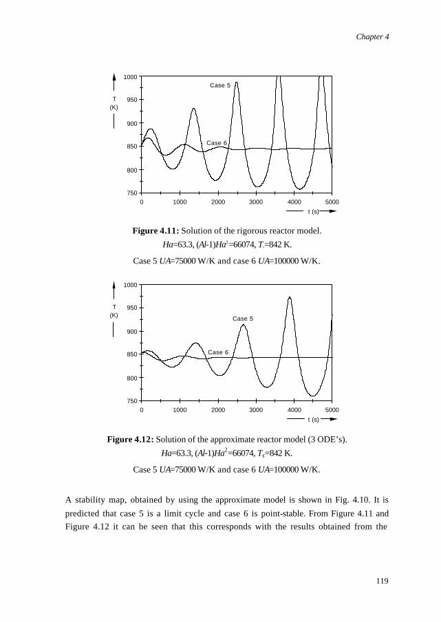
Chapter 4

119

750

800

850

900

950

1000

0 1000 2000 3000 4000 5000

t (s)

T(K)

Case 5

Case 6

Figure 4.11: Solution of the rigorous reactor model.

Ha=63.3, (Al-1)Ha2=66074, Ts=842 K.

Case 5 UA=75000 W/K and case 6 UA=100000 W/K.

750

800

850

900

950

1000

0 1000 2000 3000 4000 5000

t (s)

T(K) Case 5

Case 6

Figure 4.12: Solution of the approximate reactor model (3 ODE’s). Ha=63.3, (Al-1)Ha2=66074, Ts=842 K.

Case 5 UA=75000 W/K and case 6 UA=100000 W/K.

A stability map, obtained by using the approximate model is shown in Fig. 4.10. It is predicted that case 5 is a limit cycle and case 6 is point-stable. From Figure 4.11 and Figure 4.12 it can be seen that this corresponds with the results obtained from the

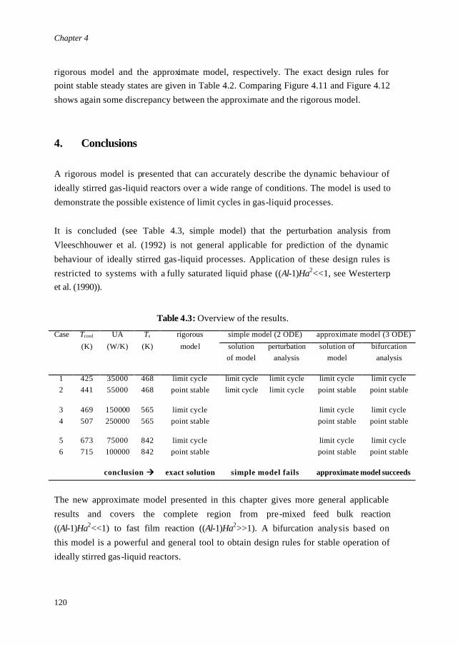
Chapter 4

120

rigorous model and the approximate model, respectively. The exact design rules for point stable steady states are given in Table 4.2. Comparing Figure 4.11 and Figure 4.12 shows again some discrepancy between the approximate and the rigorous model.

4. Conclusions A rigorous model is presented that can accurately describe the dynamic behaviour of ideally stirred gas-liquid reactors over a wide range of conditions. The model is used to demonstrate the possible existence of limit cycles in gas-liquid processes. It is concluded (see Table 4.3, simple model) that the perturbation analysis from Vleeschhouwer et al. (1992) is not general applicable for prediction of the dynamic behaviour of ideally stirred gas-liquid processes. Application of these design rules is restricted to systems with a fully saturated liquid phase ((Al-1)Ha2<<1, see Westerterp et al. (1990)).

Table 4.3: Overview of the results.

Case Tcool UA Ts rigorous simple model (2 ODE) approximate model (3 ODE)

(K) (W/K) (K) model

solution of model

perturbation analysis

solution of model

bifurcation analysis

1 2

425 441

35000 55000

468 468

limit cycle point stable

limit cycle limit cycle

limit cycle limit cycle

limit cycle point stable

limit cycle point stable

3 4

469 507

150000 250000

565 565

limit cycle point stable

limit cycle point stable

limit cycle point stable

5 6

673 715

75000 100000

842 842

limit cycle point stable

limit cycle point stable

limit cycle point stable

conclusion àà exact solution simple model fails approximate model succeeds

The new approximate model presented in this chapter gives more general applicable results and covers the complete region from pre-mixed feed bulk reaction ((Al-1)Ha2<<1) to fast film reaction ((Al-1)Ha2>>1). A bifurcation analysis based on this model is a powerful and general tool to obtain design rules for stable operation of ideally stirred gas-liquid reactors.

Chapter 4

121

The decoupling of mass and heat balances on micro scale increases the error of the approximate model and the corresponding bifurcation analysis (especially in the fast reaction regime). Therefore, the rigorous reactor model should be used to check the obtained design rules and to investigate the dynamic system behaviour more detailed.

Acknowledgement This work has been supported by DSM Research, Geleen.

Notation a specific surface area [m2 m-3] A heat transfer area [m2] A component A [-]

Al Hinterland ratio (defined by εlkl / aDa) [-] B component B [-] C component C [-] CP heat capacity [J kg -1 K-1] D component D [-] Dsubscript diffusivity [m2 s -1] Eact activation energy [J mol-1] Esubscript enhancement factor [-] hg gas phase heat transfer coefficient [W m-2 K-1]

-∆HR heat of reaction based on R [J mol-1] Ha Hatta number defined as (kR [B]Da)0.5/kl [-] Jsubscript molar flux [mol m-2 s -1] JT heat flux [W m-2] kg gas phase mass transfer coefficient [m s -1] kl liquid phase mass transfer coefficient [m s -1] kR,m,n reaction rate constant [m3(m+n-1) mol-(m+n-1) s -1] m reaction order [-] msubscript gas-liquid partition coefficient [-] n reaction order [-]

Chapter 4

122

N counter with start value 1 at t=0 [-] Nsubscript number of moles [mol] Rsubscript reaction rate [mol m-3 s -1] Rgas ideal gas constant [J mol-1 K-1] t simulation time variable [s] T temperature [K] U heat transfer coefficient [W m-2 K-1] VR reactor volume [m3] x place variable [m]

xdimensionless place variable defined as x/√(4Daθ) [-] [] concentration [mol m-3] []subscript concentration [mol m-3] Greek letters

δp assumed thickness of liquid element [m]

εg gas phase hold-up [-]

εl liquid phase hold-up [-]

Φl liquid volume flow [m3 s -1]

γsubscript stoichiometry number [-]

λ thermal conductivity [W m-1 K-1]

θ contact time according to penetration model (defined by 4Da / πkl2) [s]

ρ density [kg m-3]

τl liquid phase residence time [s] Subscripts 0 initial value a component A b component B bulk at bulk conditions c component C cool cooling medium d component D g gas phase i interface

Chapter 4

123

i species i in at inlet conditions l liquid phase s steady state value T temperature

References Aris, R. and Amundson, N.R., (1958), An analysis of chemical reactor stability and control – part I to III, Chem. Eng. Sci. 7, 121-155. Baccaro, G.P., Gaitonde, N.Y. and Douglas, J.M., (1970), An experimental study of oscillating reactors, AIChE Journal 16, 249-254. Bilous, O. and Amundson, N.R., (1955), Chemical reactor stability and sensitivity, AIChE Journal 1, 513-521. Elk, E.P. van, Borman, P.C., Kuipers, J.A.M. and Versteeg, G.F., (2000), Modelling of gas-liquid reactors – implementation of the penetration model in dynamic modelling of gas-liquid processes with the presence of a liquid bulk, Chem. Eng. J. 76, 223-237. (Chapter 3 of this thesis). Heiszwolf, J.J. and Fortuin, M.H., (1997), Design procedure for stable operations of first-order reaction systems in a CSTR, AIChE Journal 43, 1060-1068. Hoffman, L.A., Sharma, S. and Luss, D., (1975), Steady state multiplicity of adiabatic gas-liquid reactors: I. The single reactor case, AIChE Journal 21, 318-326. Huang, D. T.-J. and Varma, A., (1981), Steady-state and dynamic behavior of fast gas-liquid reactions in non-adiabatic continuous stirred tank reactors, Chem. Eng. J. 21, 47-57. Huang, D. T.-J. and Varma, A., (1981), Steady-state uniqueness and multiplicity of nonadiabatic gas-liquid CSTRs, AIChE Journal 27, 481-489.

Chapter 4

124

Olsen, R.J. and Epstein, I.R., (1993), Bifurcation analysis of chemical reaction mechanisms. II. Hopf bifurcation analysis, J. of Chem. Phys. 98, 2805-2822. Sharma, S., Hoffman, L.A. and Luss, D., (1976), Steady state multiplicity of adiabatic gas-liquid reactors: II. The two consecutive reactions case, AIChE Journal 22, 324-331. Singh, C.P.P. and Shah, Y.T., (1982), The effect of gas feed temperature on the steady state multiplicity of an adiabatic CSTR with a fast pseudo-first-order reaction, Chem. Eng. J. 23, 101-104. Swaaij, W.P.M. van and Versteeg, G.F., (1992), Mass transfer accompanied with complex reversible chemical reaction in gas-liquid systems: an overview, Chem. Eng. Sci. 47, 3181-3195. Uppal, A., Ray, W.H. and Poore, A.B., (1974), On the dynamic behavior of continuous stirred tank reactors, Chem. Eng. Sci. 29, 967-985. Uppal, A., Ray, W.H. and Poore, A.B., (1976), The classification of the dynamic behavior of continuous sirred tank reactors – Influence of reactor residence time, Chem. Eng. Sci. 31, 205-214. Vas Bhat, R.D., Swaaij, W.P.M. van, Benes, N.E., Kuipers, J.A.M. and Versteeg, G.F., (1997), Non-isothermal gas absorption with reversible chemical reaction, Chem. Eng. Sci. 52, 4079-4094. Vejtassa, S.A. and Schmitz, R.A., (1970), An experimental study of steady state multiplicity and stability in an adiabatic stirred reactor, AIChE Journal 16, 410-419. Vleeschhouwer, P.H.M. and Fortuin, J.M.H., (1990), Theory and experiments concerning the stabilty of a reacting system in a CSTR, AIChE Journal 36, 961-965. Vleeschhouwer, P.H.M., Garton, R.D. and Fortuin, J.M.H., (1992), Analysis of limit cycles in an industrial oxo reactor, Chem. Eng. Sci. 47, 2547-2552.

Chapter 4

125

Westerterp, K.R., Swaaij, W.P.M. van and Beenackers, A.A.C.M., (1990), Chemical Reactor Design and Operation, Wiley, New York.

Chapter 4

126

127

CHAPTER 5

Stability and dynamic behaviour of a

hydroformylation reactor – Influence of mass

transfer in the kinetics controlled regime

5. Stability and dynamic behaviour of a

hydroformylation reactor – Influence of mass

transfer in the kinetics controlled regime

Chapter 5

128

Abstract In behalf of the development of new hydroformylation reactors, a study was initiated to examine the dynamics of hydroformylation processes. The current chapter presents the results of applying the rigorous reactor model (van Elk et al., 1999 and 2000) and the approximate reactor model (van Elk et al., 1999) on a new, to be developed, hydroformylation reactor with complex kinetics. The reaction considered is first order in the olefin and the catalyst concentration, while the apparent reaction order in hydrogen (H2) varies between 0 and 1 and in carbon monoxide (CO) between -1 and 1, depending on the hydrogen and carbon monoxide concentrations respectively. The influence of the cooler design and the mass transfer on the dynamic behaviour is investigated in the kinetic controlled regime. It is shown that this reactor will show oscillatory behaviour under certain realistic operating conditions. From stability analysis it was found that the desired steady state (temperature, conversion) exists for a wide range of mass transfer parameters. However, the cases are only statically similar, but dynamically show an important difference: for some conditions the steady state is found to be dynamically stable, while for other conditions the same steady state is found to be dynamically unstable (limit cycle). This unusual phenomenon is possible due to the negative reaction order in CO.

Chapter 5

129

1. Introduction With respect to the development of a new hydroformylation reactor, a study was initiated to examine the dynamics of hydroformylation processes. The dynamic behaviour of a reactor in general and especially of a hydroformylation reactor is a very important part of the reactor design. A literature survey indicated that undesired sustained temperature oscillations may exist in hydroformylation reactors under certain circumstances (Vleeschhouwer et al., 1992). In plant operation, these conditions have to be avoided because they may adversely affect product quality, catalyst degradation and downstream operations and can lead to serious difficulty in process control and unsafe reactor operations. Two models to be used as design tools have been developed and validated: 1. A rigorous reactor model (van Elk et al., 1999 and 2000). 2. An approximate reactor model for stability analysis (van Elk et al., 1999). The models are used to investigate the influence of the cooler design and the mass transfer coefficient and/or contact area on the stability and dynamic behaviour of the reactor. The rigorous model (van Elk et al., 1999 and 2000) requires a minimum amount of model assumptions and simplifications moreover it takes all relevant phenomena into account. The rigorous model is based on the following major assumptions: 1. The mass transfer in the gas phase is described with the stagnant film model. 2. The mass transfer in the liquid phase is described with the Higbie (Higbie, 1935)

penetration model. 3. The contact time according to the penetration model is small compared to the

liquid-phase residence time. 4. Both the gas and the liquid-phase are assumed to be perfectly mixed (i.e. CISTRs). The approximate model (van Elk et al., 1999) is a much simpler one based on some additional assumptions. This model takes only the key phenomena into account. The model consists of liquid-phase material balances (ordinary differential equations) and an approximate algebraic expression for the enhancement factor. The approximate model is based on the following additional assumptions:

Chapter 5

130

1. The influence of mass transfer is sufficiently accurate described by an approximate and explicit analytical expression for the enhancement factor (Ea).

2. The influence of temperature profiles on micro scale can be neglected. 3. The resistance to mass transfer in the gas-phase can be neglected. 4. The influence of the gas phase heat balance can be neglected or alternatively the

gas and liquid phase heat balances can be combined into one overall heat balance. 5. The gas-phase concentration is constant or alternatively the gas-phase partial

pressure is constant. This assumption is fulfilled when a sufficiently fast partial pressure regulation is present.

The approximate model is very useful to create stability maps from which design rules for stable operation can be obtained. Using the more accurate rigorous model as a final check-up for the chosen set of operating conditions is however recommended. Illustrative examples (van Elk et al., 1999) showed that for fictitious gas-liquid reactors, with simple first or second order kinetics, operating conditions can be created where oscillations (limit cycles) are found. It was also shown that the approximate model is a very useful tool for predicting the regions where instabilities take place and more important to find design rules which ensure stable operation. The current study presents the results of applying both the rigorous and the approximate reactor model on a hydroformylation process with more complex kinetics. It is shown that this reactor will show oscillatory behaviour under certain realistic operating conditions. The current study thus shows that limit cycles can be expected to exist for real industrial designs and not only for fictitious non-existing reactors and/or processes.

2. Theory 2.1 Introduction

Hydroformylation is a chemical process in which the addition of hydrogen and carbon monoxide to an olefinic double bond takes place. The product is a mixture of normal- and iso-aldehyde and alcohols. The hydroformylation reaction is catalysed homogeneously by Group VIII metals (e.g. Ir, Co, Rh). The introduction of various ligands to the catalyst (e.g. Co2(CO)6[P(n-C4H9)3]2) and the operating conditions (i.e.

Chapter 5

131

pressure, temperature and CO/H2-ratio) can have a significant influence on the selectivity. The problem considered is a gas-liquid hydroformylation reactor with mass transfer of hydrogen and carbon monoxide, followed by an irreversible reaction of complex kinetics:

)aldehyde()olefine( )(CO )(H 2 llgg →++ (5.1) The complex kinetics equation used in this study is:

( ) ( )2CO2H2

2/0 ][1

][][1

][]][[COK

COHK

HcatalystolefinekR RTER

act

++= − (5.2)

Thus, the reaction is assumed to be first order in the olefin and catalyst concentration, while the apparent reaction order in H2 can vary between 0 and 1 and in CO between -1 and 1, depending on the hydrogen and carbon monoxide concentrations respectively. Due to e.g. economical and technical reasons for the reactor design the following design constraints are assumed: 1. Total gas phase pressure about 10 bar. 2. Molar H2/CO-ratio in gas-phase near unity. 3. Operating temperature of about 100 °C. 4. Catalyst concentration of 0.5 mol/m3. 5. Conversion of about 50%. 6. Mass transfer rate (kla) between 0.025 and 0.2 1/s. 7. Cooling capacity UA and cooling temperature Tcool to be determined for stable

operation. The chosen kinetic data and operating conditions of the reactor are representative for a family of hydroformylation processes. 2.2 Rigorous model

The rigorous reactor model as described by van Elk et al. (1999 and 2000) considers all species on micro as well as on macro scale. However, over 99% of the calculation time is required for the micro scale model (i.e. the Higbie penetration model). To reduce the

Chapter 5

132

required calculation time almost by a factor two it was decided to include only species H2, CO and olefin in the micro model used for the hydroformylation reactor model. The other species and parameters (i.e. temperature, aldehyde and catalyst) are considered on macro scale only. This simplification is allowed for this specific hydroformylation process provided that: 1. The influence of the temperature profile on micro scale is negligible due to a good

heat transfer between the gas and the liquid phase. 2. The reaction is irreversible, so that the aldehyde concentration does not influence

the reaction rate. 3. The catalyst concentration will be constant all over the reactor on micro as well as

on macro scale. The micro model for the phenomenon mass transfer accompanied by a chemical reaction is thus governed by the following equations:

RxHD

tH −=

22

2

H22 ][][

∂∂

∂∂ (5.3)

RxCOD

tCO −=

2

2

CO][][

∂∂

∂∂ (5.4)

Rx

olefinDt

olefin −=2

2

olefin][][

∂∂

∂∂ (5.5)

To permit a unique solution of the non-linear partial differential equations (5.3) to (5.5) one initial (5.6) and two boundary conditions (5.7) and (5.8) are required:

olefin CO,,Hi where,][][:0and0 2bulk, ==≥= liixt (5.6)

olefin CO, ,H i where,]i[]i[ :and0 2bulk, ===> lpxt δ (5.7)

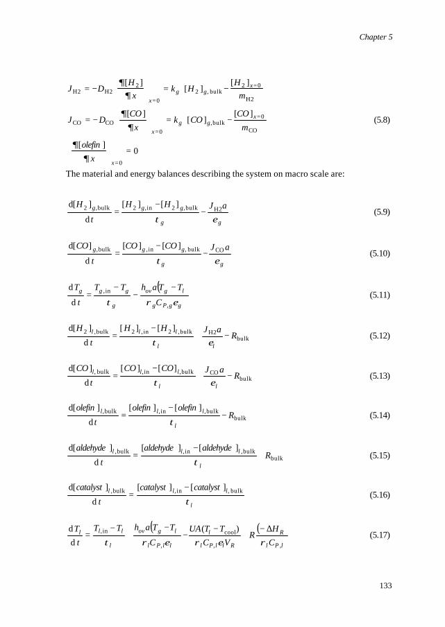
Chapter 5

133

0][

][][

][

][][

][

0

CO

0bulk,

0COCO

H2

02bulk,2

0

2H2H2

=

−=

−=

−=

−=

=

=

=

=

=

x

xgg

x

xgg

x

xolefin

mCO

COkx

CODJ

mH

Hkx

HDJ

∂∂

∂∂

∂∂

(5.8)

The material and energy balances describing the system on macro scale are:

gg

ggg aJHH

t

H

ετH2bulk,2in,2bulk,2 ][][

d

]d[−

−= (5.9)

gg

ggg aJCOCO

t

CO

ετCObulk,in,bulk, ][][

d

]d[−

−= (5.10)

( )ggPg

lgov

g

ggg

C

TTahTT

t

T

ερτ ,

in,

d

d −−

−= (5.11)

bulkH2bulk,2in,2bulk,2 ][][

d

]d[R

aJHH

t

H

ll

lll −+−

=ετ

(5.12)

bulkCObulk,in,bulk, ][][

d

]d[R

aJCOCO

t

CO

ll

lll −+−

=ετ

(5.13)

bulkbulk,in,bulk, ][][

d

]d[R

olefinolefin

t

olefin

l

lll −−

=τ

(5.14)

bulkbulk,in,bulk, ][][

d

]d[R

aldehydealdehyde

t

aldehyde

l

lll +−

=τ

(5.15)

l

lll catalystcatalyst

t

catalyst

τbulk,in,bulk, ][][

d

]d[ −= (5.16)

( ) ( )lPl

R

RllPl

l

llPl

lgov

l

lll

CH

RVC

TTUAC

TTahTT

tT

,,

cool

,

in, )(dd

ρερερτ∆−

+−

−−

+−

= (5.17)

Chapter 5

134

The overall rigorous mathematical model combines the micro and macro model equations (5.3) to (5.17) by simultaneously solving the micro and macro model. The macro model is coupled to the micro model by the boundary conditions. The exact numerical implementation is described and validated in Chapter 3 of this thesis (van Elk et al., 2000). 2.3 Bifurcation analysis

Bifurcation analysis is an efficient technique that allows analysis of the static and dynamic stability of processes without having to solve completely the dynamic equations describing the system. Various authors (e.g. Huang and Varma (1981a), Vleeschhouwer et al. (1992), Heiszwolf and Fortuin (1997), Van Elk et al. (1999) discuss the theory of bifurcation analysis applied on ideally stirred tank reactors. A system is considered point-stable if, after a sufficiently small perturbation from the steady state, the system returns to its initial state (i.e. asymptotic damping or spiral point, see Fig. 5.1). If the slope condition is violated the system shows static instability (extinction or ignition to a static stable point, see Fig. 5.1). If the dynamic condition is violated the system shows dynamic instability (limit cycle, see Fig. 5.1). If a stability map (like Fig. 5.3) is made with S-shaped curves of the loci of points representing the steady states of the system as a function of a certain parameter (for example the coolant temperature), two additional curves can be drawn to divide the figure in three distinct regions, each with a characteristic dynamic behaviour. The two curves are the fold bifurcation curve and the Hopf bifurcation curve. The three distinct regions are: I. region with point-stable steady states; II. region with dynamic instability (also called orbitally stable region or limit cycle region); III. region with static instability. Region I can be further divided in two separate regions by the double Eigenvalue curve (DEV). Region Ia shows asymptotic damping and region Ib spiral point behaviour. The dynamic behaviour of the system in each of the four regions is schematically shown in Fig. 5.1.

Chapter 5

135

TSS t

Region Ia - StableAsymptotic damping

T

TSS t

Regio Ib - StableSpiral point

T

TSS t

Region II - Dynamic unstableLimit cycle close to Hopf

T

TSS t

Region II - Dynamic unstableLimit cycle far from Hopf

T

TSS t

Region III - Static unstableTransition ignition

T

TSS t

Region III - Static unstableTransition extinction

T

Figure 5.1: Schematic presentation of various kinds of dynamic behaviour of a system after a step disturbance. The dotted horizontal line indicates the desired steady state.

Application of the bifurcation analysis requires simplification of the rigorous reactor model to an approximate reactor model consisting of a system of ordinary differential and algebraic equations. 2.4 Approximate model (4 ODE’s)

The rigorous reactor model is too complicated for a bifurcation analysis. Therefore, the rigorous reactor model must be simplified to an approximate model with only ordinary differential and algebraic equations. The simplest system of ODEs in agreement with the assumptions given in section 1 is (assuming that the liquid feed is free of H2 and CO):

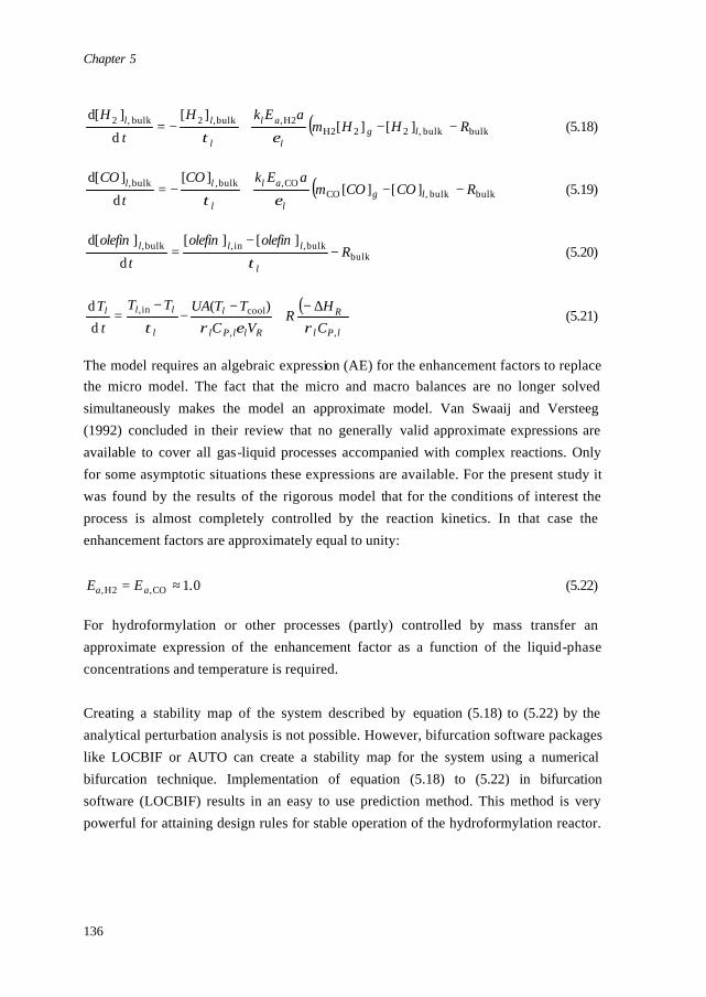
Chapter 5

136

( ) bulkbulk,22H2H2,bulk,2bulk,2 ][][

][

d

]d[RHHm

aEkH

t

Hlg

l

al

l

ll −−+−=ετ

(5.18)

( ) bulkbulk,COCO,bulk,bulk, ][][

][

d

]d[RCOCOm

aEkCO

t

COlg

l

al

l

ll −−+−=ετ

(5.19)

bulkbulk,in,bulk, ][][

d

]d[R

olefinolefin

t

olefin

l

lll −−

=τ

(5.20)

( )lPl

R

RllPl

l

l

lll

CH

RVC

TTUATT

tT

,,

coolin, )(dd

ρερτ∆−

+−

−−

= (5.21)

The model requires an algebraic expression (AE) for the enhancement factors to replace the micro model. The fact that the micro and macro balances are no longer solved simultaneously makes the model an approximate model. Van Swaaij and Versteeg (1992) concluded in their review that no generally valid approximate expressions are available to cover all gas-liquid processes accompanied with complex reactions. Only for some asymptotic situations these expressions are available. For the present study it was found by the results of the rigorous model that for the conditions of interest the process is almost completely controlled by the reaction kinetics. In that case the enhancement factors are approximately equal to unity:

0.1CO,H2, ≈= aa EE (5.22) For hydroformylation or other processes (partly) controlled by mass transfer an approximate expression of the enhancement factor as a function of the liquid-phase concentrations and temperature is required. Creating a stability map of the system described by equation (5.18) to (5.22) by the analytical perturbation analysis is not possible. However, bifurcation software packages like LOCBIF or AUTO can create a stability map for the system using a numerical bifurcation technique. Implementation of equation (5.18) to (5.22) in bifurcation software (LOCBIF) results in an easy to use prediction method. This method is very powerful for attaining design rules for stable operation of the hydroformylation reactor.

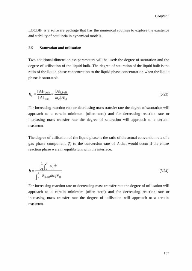
Chapter 5

137

LOCBIF is a software package that has the numerical routines to explore the existence and stability of equilibria in dynamical models. 2.5 Saturation and utilisation

Two additional dimensionless parameters will be used: the degree of saturation and the degree of utilisation of the liquid bulk. The degree of saturation of the liquid bulk is the ratio of the liquid phase concentration to the liquid phase concentration when the liquid phase is saturated:

ga

l

l

la Am

A

A

A

][

][

][

][ bulk,

sat,

bulk, ≈≡η (5.23)

For increasing reaction rate or decreasing mass transfer rate the degree of saturation will approach to a certain minimum (often zero) and for decreasing reaction rate or increasing mass transfer rate the degree of saturation will approach to a certain maximum. The degree of utilisation of the liquid phase is the ratio of the actual conversion rate of a gas phase component (A) to the conversion rate of A that would occur if the entire reaction phase were in equilibrium with the interface:

Rsat,0

0

V

1

la

a

dtR

dt

ε

ξθη θ

θ

∫∫

≈ (5.24)

For increasing reaction rate or decreasing mass transfer rate the degree of utilisation will approach to a certain minimum (often zero) and for decreasing reaction rate or increasing mass transfer rate the degree of utilisation will approach to a certain maximum.

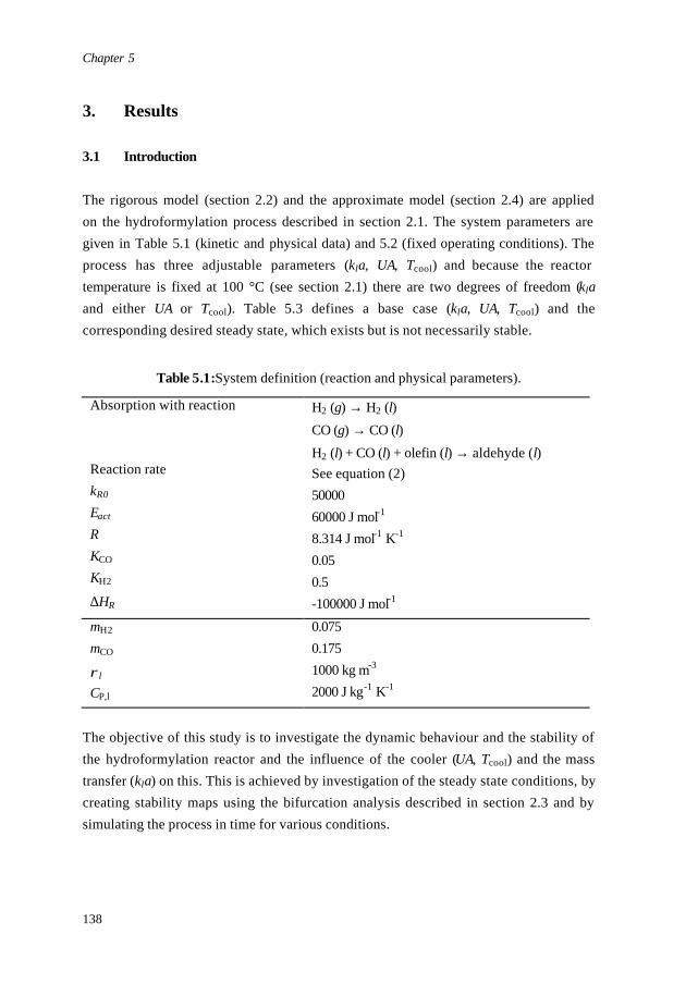
Chapter 5

138

3. Results 3.1 Introduction

The rigorous model (section 2.2) and the approximate model (section 2.4) are applied on the hydroformylation process described in section 2.1. The system parameters are given in Table 5.1 (kinetic and physical data) and 5.2 (fixed operating conditions). The process has three adjustable parameters (kla, UA, Tcool) and because the reactor temperature is fixed at 100 °C (see section 2.1) there are two degrees of freedom (kla and either UA or Tcool). Table 5.3 defines a base case (kla, UA, Tcool) and the corresponding desired steady state, which exists but is not necessarily stable.

Table 5.1:System definition (reaction and physical parameters).

Absorption with reaction Reaction rate kR0 Eact R KCO KH2

∆HR

H2 (g) → H2 (l)

CO (g) → CO (l)

H2 (l) + CO (l) + olefin (l) → aldehyde (l) See equation (2) 50000 60000 J mol-1 8.314 J mol-1 K-1 0.05 0.5 -100000 J mol-1

mH2

mCO

ρl CP,l

0.075 0.175 1000 kg m-3 2000 J kg-1 K-1

The objective of this study is to investigate the dynamic behaviour and the stability of the hydroformylation reactor and the influence of the cooler (UA, Tcool) and the mass transfer (kla) on this. This is achieved by investigation of the steady state conditions, by creating stability maps using the bifurcation analysis described in section 2.3 and by simulating the process in time for various conditions.

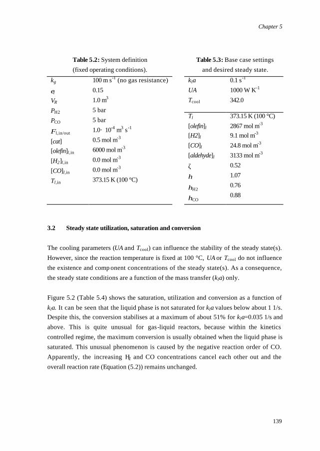
Chapter 5

139

Table 5.2: System definition (fixed operating conditions).

Table 5.3: Base case settings and desired steady state.

kla UA Tcool

0.1 s-1 1000 W K-1 342.0

kg

εl VR PH2 PCO

Φl,in/out

[cat] [olefin]l,in [H2]l,in [CO]l,in Tl,in

100 m s-1 (no gas resistance) 0.15 1.0 m3 5 bar 5 bar 1.0· 10-4 m3 s -1

0.5 mol m-3 6000 mol m-3 0.0 mol m-3 0.0 mol m-3 373.15 K (100 °C)

Tl [olefin]l [H2]l [CO]l [aldehyde]l

ζ

η

ηH2

ηCO

373.15 K (100 °C) 2867 mol m-3 9.1 mol m-3 24.8 mol m-3 3133 mol m-3 0.52 1.07 0.76 0.88

3.2 Steady state utilization, saturation and conversion

The cooling parameters (UA and Tcool) can influence the stability of the steady state(s). However, since the reaction temperature is fixed at 100 °C, UA or Tcool do not influence the existence and comp onent concentrations of the steady state(s). As a consequence, the steady state conditions are a function of the mass transfer (kla) only. Figure 5.2 (Table 5.4) shows the saturation, utilization and conversion as a function of kla. It can be seen that the liquid phase is not saturated for kla values below about 1 1/s. Despite this, the conversion stabilises at a maximum of about 51% for kla=0.035 1/s and above. This is quite unusual for gas-liquid reactors, because within the kinetics controlled regime, the maximum conversion is usually obtained when the liquid phase is saturated. This unusual phenomenon is caused by the negative reaction order of CO. Apparently, the increasing H2 and CO concentrations cancel each other out and the overall reaction rate (Equation (5.2)) remains unchanged.

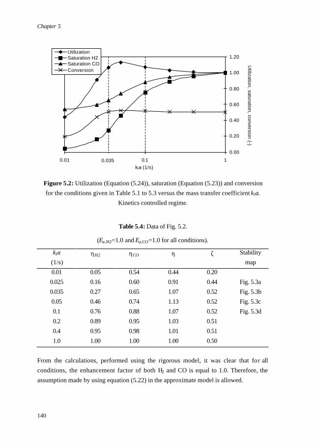
Chapter 5

140

0.00

0.20

0.40

0.60

0.80

1.00

1.20

0.01 0.1 1

kla (1/s)

Utiliza

tion

, satu

ratio

n, co

nve

rsion

(-)

UtilizationSaturation H2Saturation COConversion

0.035

Figure 5.2: Utilization (Equation (5.24)), saturation (Equation (5.23)) and conversion for the conditions given in Table 5.1 to 5.3 versus the mass transfer coefficient kla.

Kinetics controlled regime.

Table 5.4: Data of Fig. 5.2.

(Ea,H2=1.0 and Ea,CO=1.0 for all conditions).

kla (1/s)

ηH2 ηCO η ζ Stability map

0.01 0.025 0.035 0.05 0.1 0.2 0.4 1.0

0.05 0.16 0.27 0.46 0.76 0.89 0.95 1.00

0.54 0.60 0.65 0.74 0.88 0.95 0.98 1.00

0.44 0.91 1.07 1.13 1.07 1.03 1.01 1.00

0.20 0.44 0.52 0.52 0.52 0.51 0.51 0.50

Fig. 5.3a Fig. 5.3b Fig. 5.3c Fig. 5.3d

From the calculations, performed using the rigorous model, it was clear that for all conditions, the enhancement factor of both H2 and CO is equal to 1.0. Therefore, the assumption made by using equation (5.22) in the approximate model is allowed.

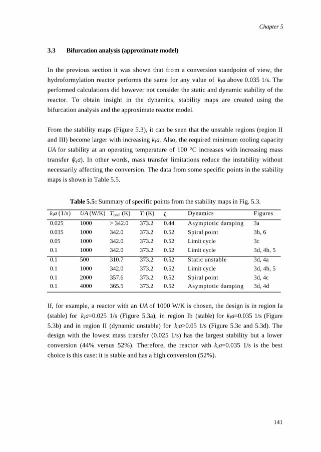
Chapter 5

141

3.3 Bifurcation analysis (approximate model)

In the previous section it was shown that from a conversion standpoint of view, the hydroformylation reactor performs the same for any value of kla above 0.035 1/s. The performed calculations did however not consider the static and dynamic stability of the reactor. To obtain insight in the dynamics, stability maps are created using the bifurcation analysis and the approximate reactor model. From the stability maps (Figure 5.3), it can be seen that the unstable regions (region II and III) become larger with increasing kla. Also, the required minimum cooling capacity UA for stability at an operating temperature of 100 °C increases with increasing mass transfer (kla). In other words, mass transfer limitations reduce the instability without necessarily affecting the conversion. The data from some specific points in the stability maps is shown in Table 5.5.

Table 5.5: Summary of specific points from the stability maps in Fig. 5.3.

k la (1/s) UA (W/K) Tcool (K) Tl (K) ζ Dynamics Figures

0.025 0.035 0.05 0.1

1000 1000 1000 1000

> 342.0 342.0 342.0 342.0

373.2 373.2 373.2 373.2

0.44 0.52 0.52 0.52

Asymptotic damping Spiral point Limit cycle Limit cycle

3a 3b, 6 3c 3d, 4b, 5

0.1 0.1 0.1 0.1

500 1000 2000 4000

310.7 342.0 357.6 365.5

373.2 373.2 373.2 373.2

0.52 0.52 0.52 0.52

Static unstable Limit cycle Spiral point Asymptotic damping

3d, 4a 3d, 4b, 5 3d, 4c 3d, 4d

If, for example, a reactor with an UA of 1000 W/K is chosen, the design is in region Ia (stable) for kla=0.025 1/s (Figure 5.3a), in region Ib (stable) for kla=0.035 1/s (Figure 5.3b) and in region II (dynamic unstable) for kla>0.05 1/s (Figure 5.3c and 5.3d). The design with the lowest mass transfer (0.025 1/s) has the largest stability but a lower conversion (44% versus 52%). Therefore, the reactor with kla=0.035 1/s is the best choice is this case: it is stable and has a high conversion (52%).

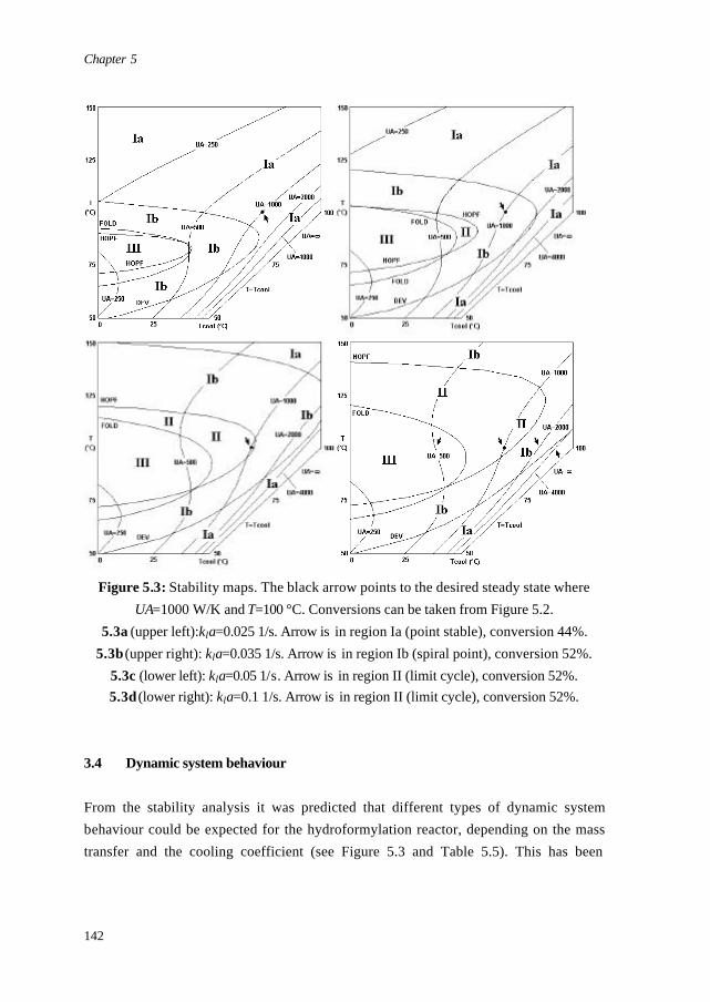
Chapter 5

142

Figure 5.3: Stability maps. The black arrow points to the desired steady state where

UA=1000 W/K and T=100 °C. Conversions can be taken from Figure 5.2. 5.3a (upper left):kla=0.025 1/s. Arrow is in region Ia (point stable), conversion 44%.

5.3b (upper right): kla=0.035 1/s. Arrow is in region Ib (spiral point), conversion 52%. 5.3c (lower left): kla=0.05 1/s. Arrow is in region II (limit cycle), conversion 52%. 5.3d (lower right): kla=0.1 1/s. Arrow is in region II (limit cycle), conversion 52%.

3.4 Dynamic system behaviour

From the stability analysis it was predicted that different types of dynamic system behaviour could be expected for the hydroformylation reactor, depending on the mass transfer and the cooling coefficient (see Figure 5.3 and Table 5.5). This has been

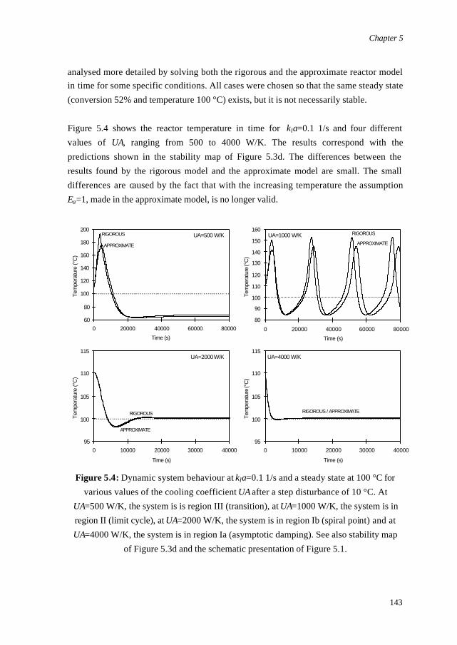
Chapter 5

143

analysed more detailed by solving both the rigorous and the approximate reactor model in time for some specific conditions. All cases were chosen so that the same steady state (conversion 52% and temperature 100 °C) exists, but it is not necessarily stable. Figure 5.4 shows the reactor temperature in time for kla=0.1 1/s and four different values of UA, ranging from 500 to 4000 W/K. The results correspond with the predictions shown in the stability map of Figure 5.3d. The differences between the results found by the rigorous model and the approximate model are small. The small differences are caused by the fact that with the increasing temperature the assumption Ea=1, made in the approximate model, is no longer valid.

60

80

100

120

140

160

180

200

0 20000 40000 60000 80000

Time (s)

Tem

pera

ture

(°C

)

RIGOROUS

APPROXIMATE

UA=500 W/K

95

100

105

110

115

0 10000 20000 30000 40000

Time (s)

Tem

pera

ture

(°C

)

APPROXIMATE

RIGOROUS

UA=2000 W/K

95

100

105

110

115

0 10000 20000 30000 40000

Time (s)

Tem

pera

ture

(°C

)

RIGOROUS / APPROXIMATE

UA=4000 W/K

80

90

100

110

120

130

140

150

160

0 20000 40000 60000 80000

Time (s)

Tem

pera

ture

(°C

)

RIGOROUS

APPROXIMATE

UA=1000 W/K

Figure 5.4: Dynamic system behaviour at kla=0.1 1/s and a steady state at 100 °C for

various values of the cooling coefficient UA after a step disturbance of 10 °C. At UA=500 W/K, the system is is region III (transition), at UA=1000 W/K, the system is in region II (limit cycle), at UA=2000 W/K, the system is in region Ib (spiral point) and at UA=4000 W/K, the system is in region Ia (asymptotic damping). See also stability map

of Figure 5.3d and the schematic presentation of Figure 5.1.

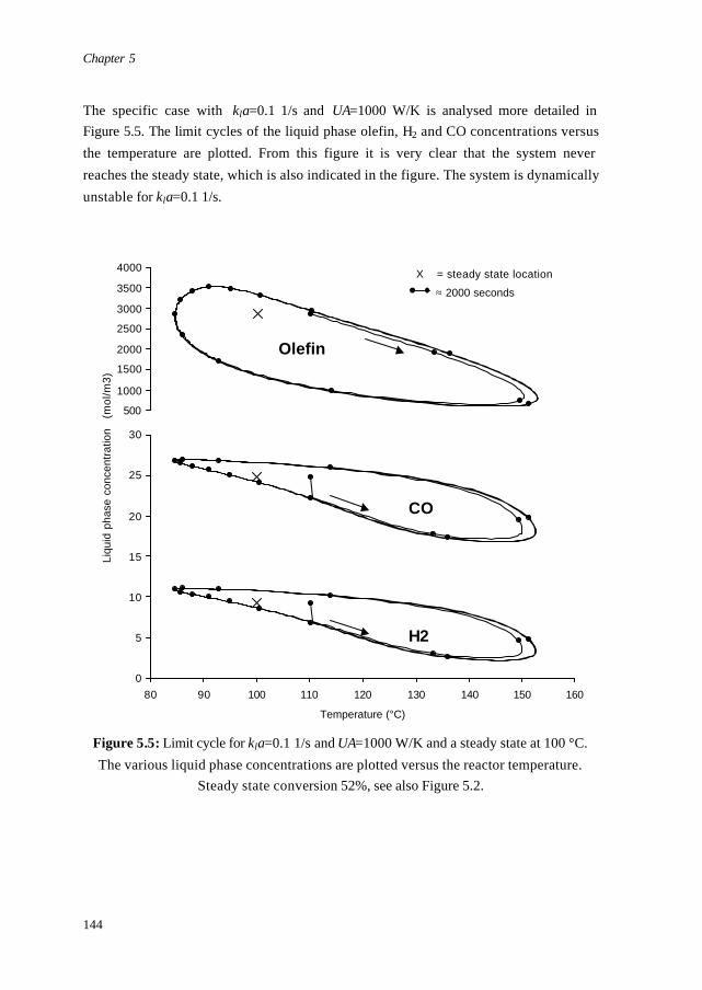
Chapter 5

144

The specific case with kla=0.1 1/s and UA=1000 W/K is analysed more detailed in Figure 5.5. The limit cycles of the liquid phase olefin, H2 and CO concentrations versus the temperature are plotted. From this figure it is very clear that the system never reaches the steady state, which is also indicated in the figure. The system is dynamically unstable for kla=0.1 1/s.

500

1000

1500

2000

2500

3000

3500

4000

(mo

l/m

3)

X = steady state location

Olefin

≈ 2000 seconds

0

5

10

15

20

25

30

80 90 100 110 120 130 140 150 160

Temperature (°C)

Liq

uid

ph

ase

co

nce

ntr

atio

n

CO

H2

Figure 5.5: Limit cycle for kla=0.1 1/s and UA=1000 W/K and a steady state at 100 °C. The various liquid phase concentrations are plotted versus the reactor temperature.

Steady state conversion 52%, see also Figure 5.2.

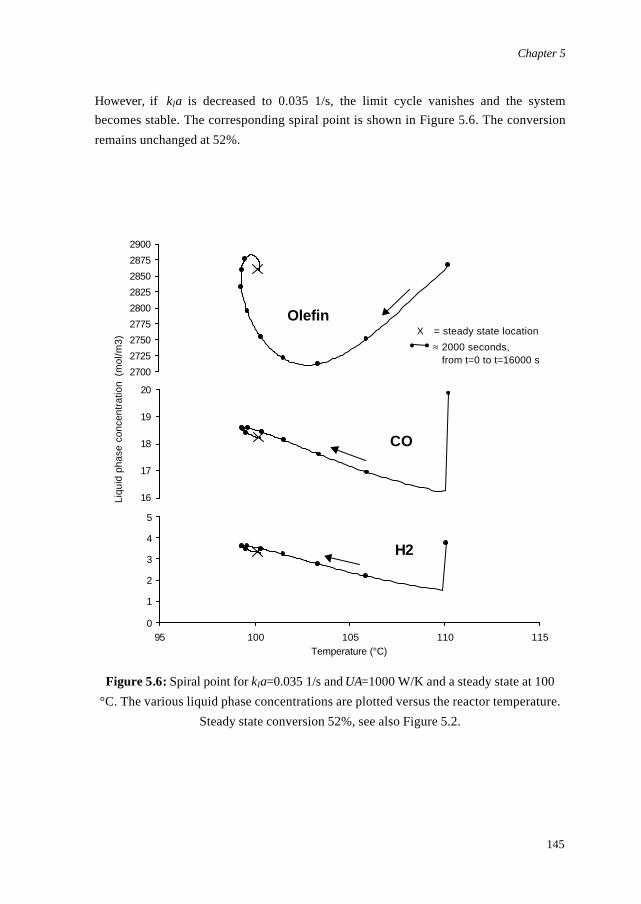
Chapter 5

145

However, if kla is decreased to 0.035 1/s, the limit cycle vanishes and the system becomes stable. The corresponding spiral point is shown in Figure 5.6. The conversion remains unchanged at 52%.

2700

2725

2750

2775

2800

2825

2850

2875

2900

(mo

l/m3

) X = steady state locationOlefin

≈ 2000 seconds, from t=0 to t=16000 s

16

17

18

19

20

Liq

uid

ph

ase

co

nce

ntr

atio

n

CO

0

1

2

3

4

5

95 100 105 110 115Temperature (°C)

H2

Figure 5.6: Spiral point for kla=0.035 1/s and UA=1000 W/K and a steady state at 100 °C. The various liquid phase concentrations are plotted versus the reactor temperature.

Steady state conversion 52%, see also Figure 5.2.

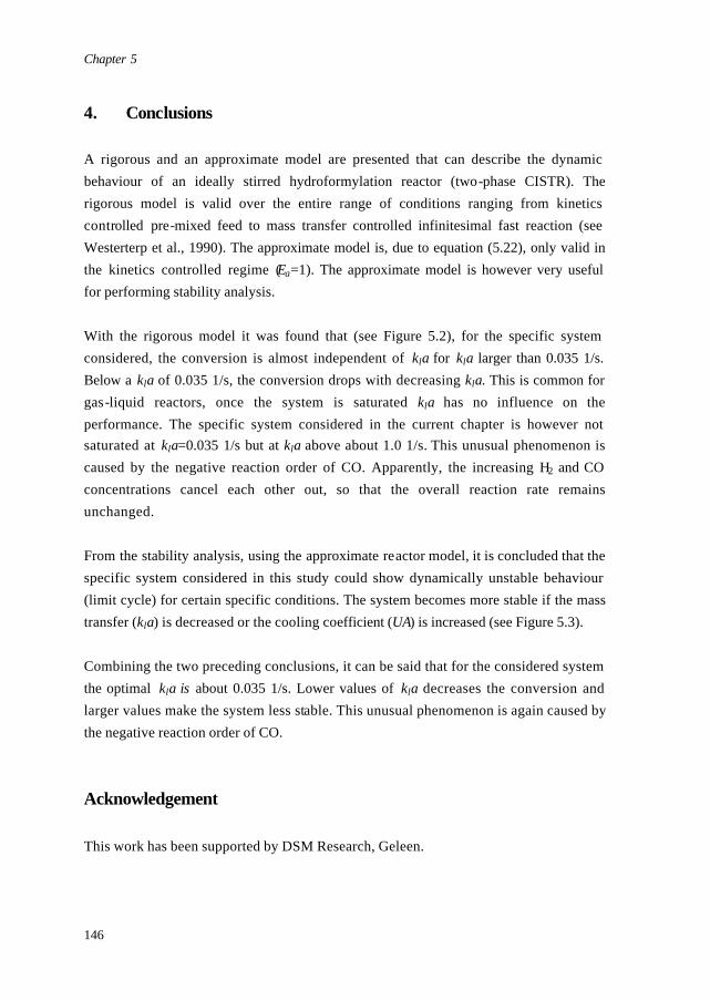
Chapter 5

146

4. Conclusions A rigorous and an approximate model are presented that can describe the dynamic behaviour of an ideally stirred hydroformylation reactor (two-phase CISTR). The rigorous model is valid over the entire range of conditions ranging from kinetics controlled pre-mixed feed to mass transfer controlled infinitesimal fast reaction (see Westerterp et al., 1990). The approximate model is, due to equation (5.22), only valid in the kinetics controlled regime (Ea=1). The approximate model is however very useful for performing stability analysis. With the rigorous model it was found that (see Figure 5.2), for the specific system considered, the conversion is almost independent of kla for kla larger than 0.035 1/s. Below a kla of 0.035 1/s, the conversion drops with decreasing kla. This is common for gas-liquid reactors, once the system is saturated kla has no influence on the performance. The specific system considered in the current chapter is however not saturated at kla=0.035 1/s but at kla above about 1.0 1/s. This unusual phenomenon is caused by the negative reaction order of CO. Apparently, the increasing H2 and CO concentrations cancel each other out, so that the overall reaction rate remains unchanged. From the stability analysis, using the approximate reactor model, it is concluded that the specific system considered in this study could show dynamically unstable behaviour (limit cycle) for certain specific conditions. The system becomes more stable if the mass transfer (kla) is decreased or the cooling coefficient (UA) is increased (see Figure 5.3). Combining the two preceding conclusions, it can be said that for the considered system the optimal kla is about 0.035 1/s. Lower values of kla decreases the conversion and larger values make the system less stable. This unusual phenomenon is again caused by the negative reaction order of CO.

Acknowledgement This work has been supported by DSM Research, Geleen.

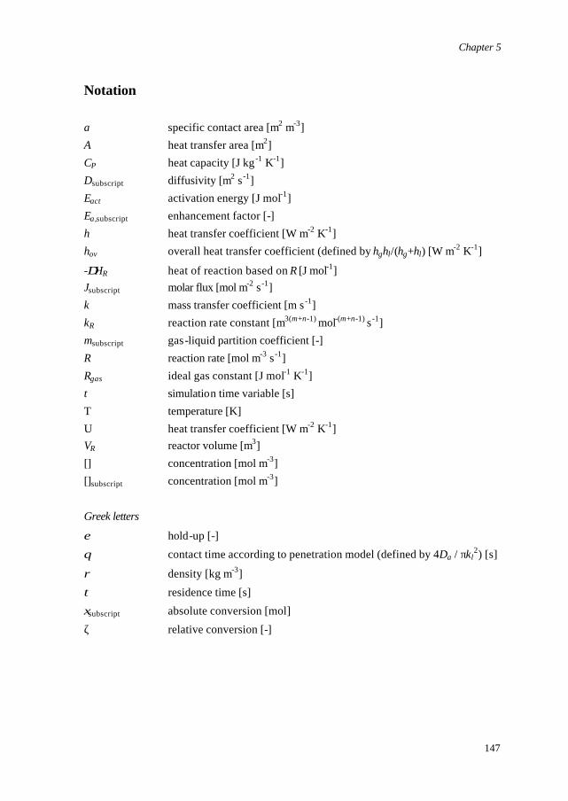
Chapter 5

147

Notation a specific contact area [m2 m-3] A heat transfer area [m2] CP heat capacity [J kg -1 K-1] Dsubscript diffusivity [m2 s -1] Eact activation energy [J mol-1] Ea,subscript enhancement factor [-] h heat transfer coefficient [W m-2 K-1] hov overall heat transfer coefficient (defined by hghl/(hg+hl) [W m-2 K-1]

-∆HR heat of reaction based on R [J mol-1] Jsubscript molar flux [mol m-2 s -1] k mass transfer coefficient [m s -1] kR reaction rate constant [m3(m+n-1) mol-(m+n-1) s -1] msubscript gas-liquid partition coefficient [-] R reaction rate [mol m-3 s -1] Rgas ideal gas constant [J mol-1 K-1] t simulation time variable [s] T temperature [K] U heat transfer coefficient [W m-2 K-1] VR reactor volume [m3] [] concentration [mol m-3] []subscript concentration [mol m-3] Greek letters

ε hold-up [-]

θ contact time according to penetration model (defined by 4Da / πkl2) [s]

ρ density [kg m-3]

τ residence time [s]

ξsubscript absolute conversion [mol]

ζ relative conversion [-]

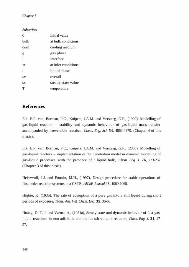
Chapter 5

148

Subscripts 0 initial value bulk at bulk conditions cool cooling medium g gas phase i interface in at inlet conditions l liquid phase ov overall ss steady state value T temperature

References Elk, E.P. van, Borman, P.C., Kuipers, J.A.M. and Versteeg, G.F., (1999), Modelling of gas-liquid reactors – stability and dynamic behaviour of gas-liquid mass transfer accompanied by irreversible reaction, Chem. Eng. Sci. 54, 4869-4879. (Chapter 4 of this thesis). Elk, E.P. van, Borman, P.C., Kuipers, J.A.M. and Versteeg, G.F., (2000), Modelling of gas-liquid reactors – implementation of the penetration model in dynamic modelling of gas-liquid processes with the presence of a liquid bulk, Chem. Eng. J. 76, 223-237. (Chapter 3 of this thesis). Heiszwolf, J.J. and Fortuin, M.H., (1997), Design procedure for stable operations of first-order reaction systems in a CSTR, AIChE Journal 43, 1060-1068. Higbie, R., (1935), The rate of absorption of a pure gas into a still liquid during short periods of exposure, Trans. Am. Inst. Chem. Eng. 35, 36-60. Huang, D. T.-J. and Varma, A., (1981a), Steady-state and dynamic behavior of fast gas-liquid reactions in non-adiabatic continuous stirred tank reactors, Chem. Eng. J. 21, 47-57.

Chapter 5

149

Swaaij, W.P.M. van and Versteeg, G.F., (1992), Mass transfer accompanied with complex reversible chemical reaction in gas-liquid systems: an overview, Chem. Eng. Sci. 47, 3181-3195. Vleeschhouwer, P.H.M., Garton, R.D. and Fortuin, J.M.H., (1992), Analysis of limit cycles in an industrial oxo reactor, Chem. Eng. Sci. 47, 2547-2552. Westerterp, K.R., Swaaij, W.P.M. van and Beenackers, A.A.C.M., (1990), Chemical Reactor Design and Operation, Wiley, New York.

Chapter 5

150

151

CHAPTER 6

The influence of staging on the stability of gas-liquid

reactors

6. The influence of staging on the stability of gas-

liquid reactors

Chapter 6

152

Abstract Prediction of the dynamic behaviour and stability of gas-liquid reactors has obtained relatively limited attention in literature. The publications available are restricted to ideally mixed reactors. In the current work, a start is made with studying the influence of macro-mixing on the dynamical behaviour of gas-liquid reactors. This is achieved by applying the methodology developed by van Elk et al. (1999) on a cascade of two reactors in series and comparing this to a single reactor of the same total volume. It is concluded that for the system investigated in this study, a cascade of two CISTRs in series provides a more stable reactor design than a single CISTR reactor. A cascade of two CISTRs results in a higher conversion and a lower minimum required cooling surface to guarantee both static an dynamic stability. It turned out that both the highest conversion and the lowest heat transfer area were obtained by putting two CISTRs of equal size in the cascade.

Chapter 6

153

1. Introduction Prediction of the dynamic behaviour of gas-liquid reactors has gained little interest in literature (Hoffman et al., 1975; Sharma et al., 1976; Huang and Varma, 1981a and 1981b; Singh et al., 1982; Vleeschhouwer et al., 1992; van Elk et al., 1999 and 2001). Only van Elk et al. (1999 and 2001) presented a methodology to predict the dynamic behaviour of ideally mixed gas-liquid reactors in all regimes from pre-mixed feed bulk reaction to fast film reaction. All authors consider only reactors that are ideally mixed with respect to both gas and liquid phase respectively, while other types of macro mixing are not considered. Also the work from van Elk et al. (1999 and 2001) is restricted to a single ideally mixed gas-liquid reactor. In this study, a start is made to investigate the influence of macro-mixing on the dynamic behaviour of gas-liquid reactors by applying the methodology presented by van Elk et al. (1999 and 2001) on a cascade of two reactors in series and comparing the results with a single reactor.

2. Theory 2.1 Introduction

The problem considered is the same as discussed in Chapter 4 of this thesis, a dynamic gas-liquid reactor with mass transfer followed by an irreversible second order chemical reaction:

(l)(l)(l)(g) dcb DCBA γγγ +→+ (6.1)

with the following overall reaction rate equation:

]][[/1,1,0 BAekR RTE

Raact−= (6.2)

The mathematical model used is based on the same assumptions as in Chapter 4 of this thesis, the only difference being that different patterns of macro mixing for the liquid phase are considered by putting two reactors in series:

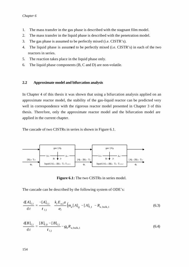
Chapter 6

154

1. The mass transfer in the gas phase is described with the stagnant film model. 2. The mass transfer in the liquid phase is described with the penetration model. 3. The gas phase is assumed to be perfectly mixed (i.e. CISTR’s). 4. The liquid phase is assumed to be perfectly mixed (i.e. CISTR’s) in each of the two

reactors in series. 5. The reaction takes place in the liquid phase only. 6. The liquid phase components (B, C and D) are non-volatile. 2.2 Approximate model and bifurcation analysis

In Chapter 4 of this thesis it was shown that using a bifurcation analysis applied on an approximate reactor model, the stability of the gas-liquid reactor can be predicted very well in correspondence with the rigorous reactor model presented in Chapter 3 of this thesis. Therefore, only the approximate reactor model and the bifurcation model are applied in the current chapter. The cascade of two CISTRs in series is shown in Figure 6.1.

gas: [A]g

VR,1 As,1

R1 J1

liquid: [A] l,1 [B] l,1 Tl,1 Tcool,1

gas: [A]g

VR,2 As,2

R2 J2

liquid: [A] l,2 [B]l,2 Tl,2 Tcool,2

[A]l,1 [B] l,1 Tl,1

Φl

[B]l,0 Tl,0

Φl

[A]l,2 [B] l,2 Tl,2

Φl

Figure 6.1: The two CISTRs in series model. The cascade can be described by the following system of ODE’s:

( ) bulk,1,,11,

1,

,11, ][][][

d

]d[alga

l

al

l

ll RAAmaEkA

t

A−−+

−=

ετ (6.3)

bulk,1,1,

,10,1, ][][

d

]d[ab

l

lll RBB

t

Bγ

τ−

−= (6.4)

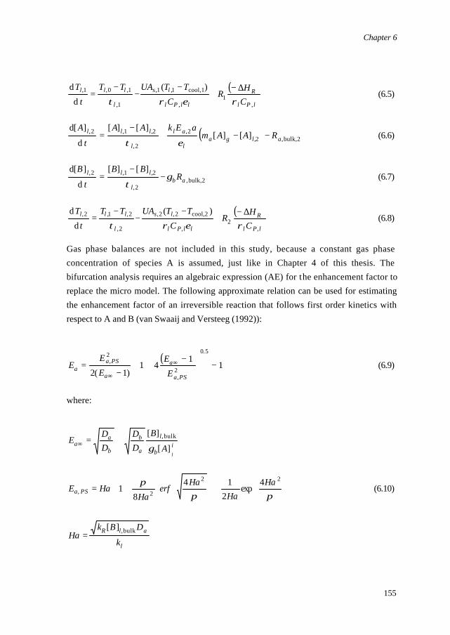
Chapter 6

155

( )lPl

R

llPl

ls

l

lll

CH

RC

TTUATT

t

T

,1

,

cool,11,1,

1,

1,0,1, )(

d

d

ρερτ∆−

+−

−−

= (6.5)

( ) bulk,2,,22,

2,

,21,2, ][][][][

d

]d[alga

l

al

l

lll RAAmaEkAA

t

A−−+

−=

ετ (6.6)

bulk,2,2,

,21,2, ][][

d

]d[ab

l

lll RBB

t

Bγ

τ−

−= (6.7)

( )lPl

R

llPl

ls

l

lll

CH

RC

TTUATT

t

T

,2

,

cool,22,2,

2,

2,1,2, )(

d

d

ρερτ∆−

+−

−−

= (6.8)

Gas phase balances are not included in this study, because a constant gas phase concentration of species A is assumed, just like in Chapter 4 of this thesis. The bifurcation analysis requires an algebraic expression (AE) for the enhancement factor to replace the micro model. The following approximate relation can be used for estimating the enhancement factor of an irreversible reaction that follows first order kinetics with respect to A and B (van Swaaij and Versteeg (1992)):

( )

−

−+

−= ∞

∞

11

41)1(2

5.0

2,

2,

PSa

a

a

PSaa E

EE

EE (6.9)

where:

ib

l

a

b

b

aa

lA

B

DD

DD

E][

][ bulk,

γ+=∞

+

+=

πππ 22

2,4

exp2

14

81

HaHa

Haerf

HaHaE PSa (6.10)

l

alR

k

DBkHa bulk,][

=

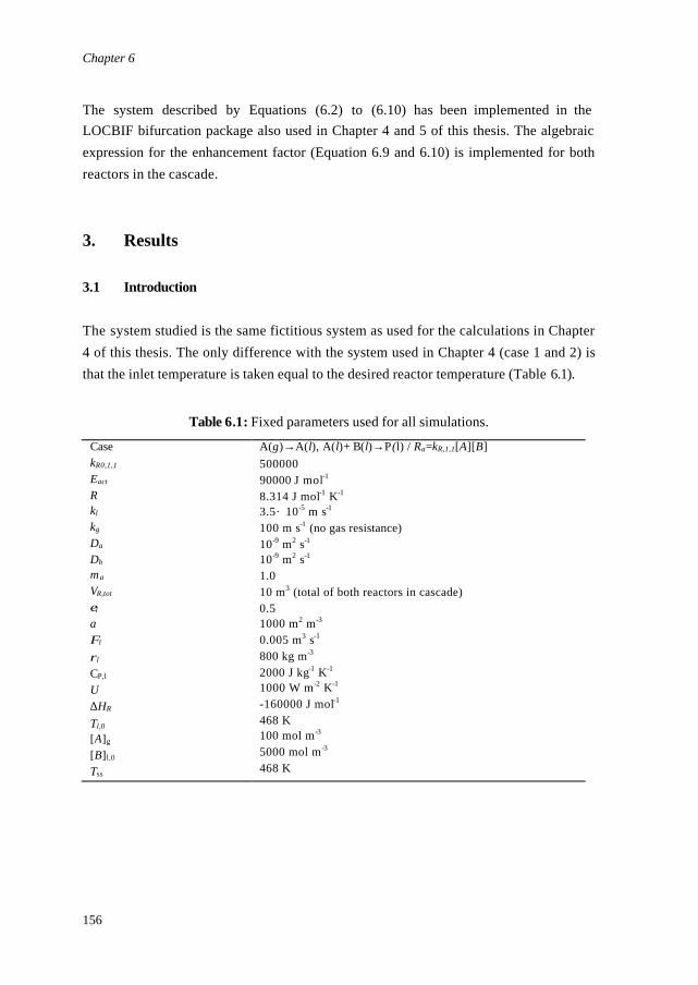
Chapter 6

156

The system described by Equations (6.2) to (6.10) has been implemented in the LOCBIF bifurcation package also used in Chapter 4 and 5 of this thesis. The algebraic expression for the enhancement factor (Equation 6.9 and 6.10) is implemented for both reactors in the cascade.

3. Results 3.1 Introduction

The system studied is the same fictitious system as used for the calculations in Chapter 4 of this thesis. The only difference with the system used in Chapter 4 (case 1 and 2) is that the inlet temperature is taken equal to the desired reactor temperature (Table 6.1).

Table 6.1: Fixed parameters used for all simulations.

Case kR0,1,1 Eact R kl kg Da Db m a VR,tot εl a Φl

ρl CP,l U ∆HR Tl,0

[A]g

[B]l,0 Tss

A(g)→A(l), A(l)+ B(l)→P(l) / Ra=kR,1,1[A][B] 500000 90000 J mol-1 8.314 J mol-1 K-1 3.5· 10-5 m s-1 100 m s-1 (no gas resistance) 10-9 m2 s-1 10-9 m2 s-1 1.0 10 m3 (total of both reactors in cascade) 0.5 1000 m2 m-3 0.005 m3 s-1

800 kg m-3 2000 J kg-1 K-1 1000 W m-2 K-1 -160000 J mol-1 468 K 100 mol m-3 5000 mol m-3 468 K

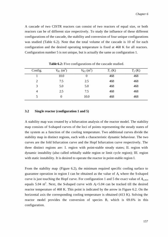
Chapter 6

157

A cascade of two CISTR reactors can consist of two reactors of equal size, or both reactors can be of different size respectively. To study the influence of these different configurations of the cascade, the stability and conversion of four unique configurations was studied (Table 6.2). Note that the total volume of the cascade is 10 m3 for each configuration and the desired operating temperature is fixed at 468 K for all reactors. Configuration number 5 is not unique, but is actually the same as configuration 1.

Table 6.2: Five configurations of the cascade studied.

Config. VR1 (m3) VR2 (m3) T1 (K) T2 (K)

1 2 3 4 5

10.0 7.5 5.0 2.5 0

0 2.5 5.0 7.5 10.0

468 468 468 468 468

468 468 468 468 468

3.2 Single reactor (configuration 1 and 5)

A stability map was created by a bifurcation analysis of the reactor model. The stability map consists of S-shaped curves of the loci of points representing the steady states of the system as a function of the cooling temperature. Two additional curves divide the stability map in distinct regions, each with a characteristic dynamic behaviour. The two curves are the fold bifurcation curve and the Hopf bifurcation curve respectively. The three distinct regions are: I. region with point-stable steady states; II. region with dynamic instability (also called orbitally stable region or limit cycle region); III. region with static instability. It is desired to operate the reactor in point-stable region I. From the stability map (Figure 6.2), the minimum required specific cooling surface to guarantee operation in region I can be obtained as the value of As where the S-shaped curve is just touching the Hopf curve. For configuration 1 and 5 the exact value of As,min equals 5.04 m-1. Next, the S-shaped curve with As=5.04 can be tracked till the desired reactor temperature of 468 K. This point is indicated by the arrow in Figure 6.2. On the horizontal axis the corresponding cooling temperature is obtained (413 K). Solving the reactor model provides the conversion of species B, which is 69.6% in this configuration.

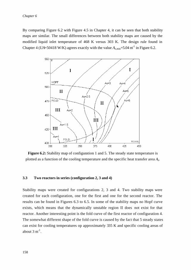
Chapter 6

158

By comparing Figure 6.2 with Figure 4.5 in Chapter 4, it can be seen that both stability maps are similar. The small differences between both stability maps are caused by the modified liquid inlet temperature of 468 K versus 303 K. The design rule found in Chapter 4 (UA=50418 W/K) agrees exactly with the value As,min=5.04 m-1 in Figure 6.2.

Figure 6.2: Stability map of configuration 1 and 5. The steady state temperature is plotted as a function of the cooling temperature and the specific heat transfer area As.

3.3 Two reactors in series (configuration 2, 3 and 4)

Stability maps were created for configurations 2, 3 and 4. Two stability maps were created for each configuration, one for the first and one for the second reactor. The results can be found in Figures 6.3 to 6.5. In some of the stability maps no Hopf curve exists, which means that the dynamically unstable region II does not exist for that reactor. Another interesting point is the fold curve of the first reactor of configuration 4. The somewhat different shape of the fold curve is caused by the fact that 5 steady states can exist for cooling temperatures op approximately 335 K and specific cooling areas of about 3 m-1.

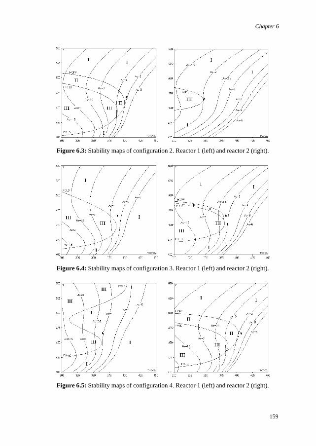
Chapter 6

159

Figure 6.3: Stability maps of configuration 2. Reactor 1 (left) and reactor 2 (right).

Figure 6.4: Stability maps of configuration 3. Reactor 1 (left) and reactor 2 (right).

Figure 6.5: Stability maps of configuration 4. Reactor 1 (left) and reactor 2 (right).

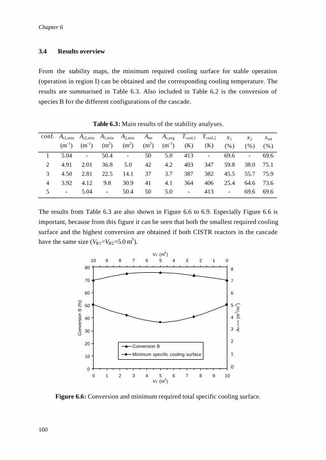
Chapter 6

160

3.4 Results overview

From the stability maps, the minimum required cooling surface for stable operation (operation in region I) can be obtained and the corresponding cooling temperature. The results are summarised in Table 6.3. Also included in Table 6.2 is the conversion of species B for the different configurations of the cascade.

Table 6.3: Main results of the stability analyses.

conf. As1,min (m-1)

As2,min (m-1)

A1,min (m2)

A2,min (m2)

Atot

(m2) As,avg (m-1)

Tcool,1

(K) Tcool,2

(K) ξ1

(%) ξ2

(%) ξtot (%)

1 2 3 4 5

5.04 4.91 4.50 3.92

-

- 2.01 2.81 4.12 5.04

50.4 36.8 22.5 9.8 -

- 5.0 14.1 30.9 50.4

50 42 37 41 50

5.0 4.2 3.7 4.1 5.0

413 403 387 364

-

- 347 382 406 413

69.6 59.8 45.5 25.4

-

- 38.0 55.7 64.6 69.6

69.6 75.1 75.9 73.6 69.6

The results from Table 6.3 are also shown in Figure 6.6 to 6.9. Especially Figure 6.6 is important, because from this figure it can be seen that both the smallest required cooling surface and the highest conversion are obtained if both CISTR reactors in the cascade have the same size (VR1=VR2=5.0 m3).

0

10

20

30

40

50

60

70

80

0 1 2 3 4 5 6 7 8 9 10V2 (m3)

Con

vers

ion

B (

%)

012345678910V1 (m3)

As

,min (

m2 /m

3 )

Conversion B

Minimum specific cooling surface

8

7

6

5

4

3

2

1

0

Figure 6.6: Conversion and minimum required total specific cooling surface.

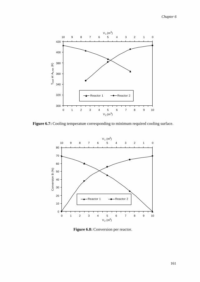
Chapter 6

161

300

320

340

360

380

400

420

0 1 2 3 4 5 6 7 8 9 10

V2 (m3)

T coo

l at

As,

min

(K

)

012345678910

V1 (m3)

Reactor 1 Reactor 2

Figure 6.7: Cooling temperature corresponding to minimum required cooling surface.

0

10

20

30

40

50

60

70

80

0 1 2 3 4 5 6 7 8 9 10

V2 (m3)

Co

nve

rsio

n B

(%

)

012345678910

V1 (m3)

Reactor 1 Reactor 2

Figure 6.8: Conversion per reactor.

Chapter 6

162

0

1

2

3

4

5

6

0 1 2 3 4 5 6 7 8 9 10

V2 (m3)

As,

min

(m

2/m

3)

012345678910

V1 (m3)

Reactor 1 Reactor 2

Figure 6.9: Minimum required specific cooling surface per reactor.

3.5 Discussion

From Table 6.3 and Figure 6.6 it can be seen that configuration 3 leads to the smallest requirements for the heat transfer area and also yields the highest conversion. The first and second reactor requires slightly different cooling temperatures (387 and 382 respectively), which may not be very practical. However, the cooling surfaces presented in Table 6.3 are minimum values and can be increased if desired. Slightly increasing the heat transfer area of the second reactor in the cascade from 14 to 15 m2 will increase the required cooling temperature of that reactor to 387 K, so that both reactors can use the same cooling medium. The total required cooling surface would then become 38 m2.

4. Conclusions A start is made by investigating the influence of macro mixing on the dynamic stability of gas-liquid reactors. It is concluded that for the system investigated in this study, a cascade of two CISTRs in series provides a more stable reactor design than a single

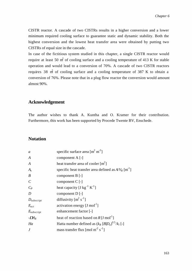
Chapter 6

163

CISTR reactor. A cascade of two CISTRs results in a higher conversion and a lower minimum required cooling surface to guarantee static and dynamic stability. Both the highest conversion and the lowest heat transfer area were obtained by putting two CISTRs of equal size in the cascade. In case of the fictitious system studied in this chapter, a single CISTR reactor would require at least 50 m2 of cooling surface and a cooling temperature of 413 K for stable operation and would lead to a conversion of 70%. A cascade of two CISTR reactors requires 38 m2 of cooling surface and a cooling temperature of 387 K to obtain a conversion of 76%. Please note that in a plug flow reactor the conversion would amount almost 90%.

Acknowledgement The author wishes to thank A. Kuntha and O. Kramer for their contribution. Furthermore, this work has been supported by Procede Twente BV, Enschede.

Notation a specific surface area [m2 m-3] A component A [-] A heat transfer area of cooler [m2] As specific heat transfer area defined as A/VR [m-1] B component B [-] C component C [-] CP heat capacity [J kg -1 K-1] D component D [-] Dsubscript diffusivity [m2 s -1] Eact activation energy [J mol-1] Esubscript enhancement factor [-]

-∆HR heat of reaction based on R [J mol-1] Ha Hatta number defined as (kR [B]Da)0.5/kl [-] J mass transfer flux [mol m-2 s -1]

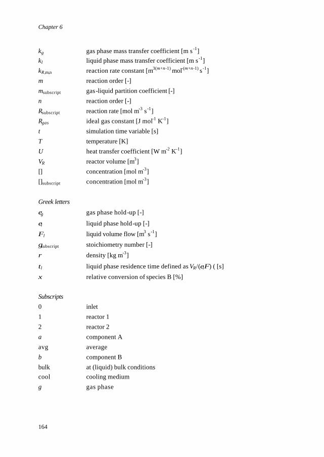
Chapter 6

164

kg gas phase mass transfer coefficient [m s -1] kl liquid phase mass transfer coefficient [m s -1] kR,m,n reaction rate constant [m3(m+n-1) mol-(m+n-1) s -1] m reaction order [-] msubscript gas-liquid partition coefficient [-] n reaction order [-] Rsubscript reaction rate [mol m-3 s -1] Rgas ideal gas constant [J mol-1 K-1] t simulation time variable [s] T temperature [K] U heat transfer coefficient [W m-2 K-1] VR reactor volume [m3] [] concentration [mol m-3] []subscript concentration [mol m-3] Greek letters

εg gas phase hold-up [-]

εl liquid phase hold-up [-]

Φl liquid volume flow [m3 s -1]

γsubscript stoichiometry number [-]

ρ density [kg m-3]

τl liquid phase residence time defined as VR/(εlΦ) ( [s]

ξ relative conversion of species B [%] Subscripts 0 inlet 1 reactor 1 2 reactor 2 a component A avg average b component B bulk at (liquid) bulk conditions cool cooling medium g gas phase

Chapter 6

165

l liquid phase min minimum ss steady state value T temperature

References Elk, E.P. van, Borman, P.C., Kuipers, J.A.M. and Versteeg, G.F., (1999), Modelling of gas-liquid reactors – stability and dynamic behaviour of gas-liquid mass transfer accompanied by irreversible reaction, Chem. Eng. Sci. 54, 4869-4879. (Chapter 4 of this thesis) Elk, E.P. van, Borman, P.C., Kuipers, J.A.M. and Versteeg, G.F., (2001), Modelling of gas-liquid reactors – stability and dynamic behaviour of a hydroformylation reactor - influence of mass transfer in the kinetics controlled regime, Chem. Eng. Sci. 56, 1491-1500. (Chapter 5 of this thesis) Hoffman, L.A., Sharma, S. and Luss, D., (1975), Steady state multiplicity of adiabatic gas-liquid reactors: I. The single reactor case, AIChE Journal 21, 318-326. Huang, D. T.-J. and Varma, A., (1981a), Steady-state and dynamic behavior of fast gas-liquid reactions in non-adiabatic continuous stirred tank reactors, Chem. Eng. J. 21, 47-57. Huang, D. T.-J. and Varma, A., (1981b), Steady-state uniqueness and multiplicity of nonadiabatic gas-liquid CSTRs, AIChE Journal 27, 481-489. Sharma, S., Hoffman, L.A. and Luss, D., (1976), Steady state multiplicity of adiabatic gas-liquid reactors: II. The two consecutive reactions case, AIChE Journal 22, 324-331. Swaaij, W.P.M. van and Versteeg, G.F., (1992), Mass transfer accompanied with complex reversible chemical reaction in gas-liquid systems: an overview, Chem. Eng. Sci. 47, 3181-3195.

Chapter 6

166

Vleeschhouwer, P.H.M., Garton, R.D. and Fortuin, J.M.H., (1992), Analysis of limit cycles in an industrial oxo reactor, Chem. Eng. Sci. 47, 2547-2552.

167

Publications This thesis

Elk, E.P. van, Borman, P.C., Kuipers, J.A.M. and Versteeg, G.F., (1999), Modelling of gas-liquid reactors – stability and dynamic behaviour of gas-liquid mass transfer accompanied by irreversible reaction, Chem. Eng. Sci. 54, 4869-4879. Elk, E.P. van, Borman, P.C., Kuipers, J.A.M. and Versteeg, G.F., (2000), Modelling of gas-liquid reactors – implementation of the penetration model in dynamic modelling of gas-liquid processes with the presence of a liquid bulk, Chem. Eng. J. 76, 223-237. Elk, E.P. van, Borman, P.C., Kuipers, J.A.M. and Versteeg, G.F., (2001), Modelling of gas-liquid reactors – stability and dynamic behaviour of a hydroformylation reactor - influence of mass transfer in the kinetics controlled regime, Chem. Eng. Sci. 56, 1491-1500. Elk, E.P. van, Knaap, M.C. and Versteeg, G.F., (2002), Application of the penetration theory for gas-liquid mass transfer in systems without a liquid bulk, submitted for publication to Chem. Eng. Comm. Other work

Knaap, M.C., Oude Lenferink, J.E., Versteeg, G.F. and Elk, E.P. van, (2000), Differences in local absorption rates of CO2 as observed in numerically comparing tray columns and packed columns, 79th annual Gas Processors Association convention, 82-94.

Publications

168

169

Dankwoord Bij wetenschappelijke publicaties is het niet ongebruikelijk dat er drie, vier of zelfs vijf auteurs worden vermeld. Op de omslag van een proefschrift wordt echter slechts één naam vermeld, terwijl juist een proefschrift een stukje werk is dat slechts tot stand kan komen dankzij de inspanning van velen. In dit deel van het proefschrift, ongetwijfeld het meest gelezen deel, wil ik hen bedanken. Als eerste wil ik mijn promotor, Geert Versteeg, bedanken voor het gestelde vertrouwen en het bieden van de gelegenheid een promotieonderzoek uit te voeren. Minstens zo belangrijk is de bijdrage van Hans Kuipers geweest, waarvoor eveneens mijn dank. Zonder de releverende discussies met Geert over stofoverdracht en vloeistofpakketjes en met Hans over partiële differentiaalvergelijkingen met differentiërende randvoorwaarden was dit proefschrift nooit tot stand gekomen. Mijn promotieonderzoek was onmogelijk geweest zonder de steun van DSM Research te Geleen. In het bijzonder de prettige contacten met Peter Borman waren zeer constructief en stimulerend. Ik wil Peter dan ook bedanken voor het gestelde vertrouwen en voor zijn inbreng in dit proefschrift. Daarnaast ben ik erg blij dat Peter in de promotiecommissie plaats heeft willen nemen als referent. Tevens bedank ik Bart Smits, die in een later stadium feilloos een aantal van de taken van Peter heeft overgenomen. Bart, die bovendien onverstoorbaar de wat ondankbare taak uitvoerde om goedkeuring te regelen voor publicatie van een artikel waarvan hij zelf geen coauteur was. Ook de steun van Shell Global Solutions International te Amsterdam heeft bijgedragen aan het tot stand komen van een deel van dit proefschrift. In dit verband noem ik in het bijzonder Mariëtte Knaap, die wellicht een veel grotere inbreng heeft gehad bij één van de publicaties dan zij zich bewust is. Mariëtte, tevens bedankt voor je enthousiasme en morele steun. In de vorm van afstudeeropdrachten, stageplaatsen en jaaropdrachten werd een belangrijke bijdrage geleverd door Jelle Ernst Oude Lenferink, Apirome Kuntha en Onno Kramer. Aan Jelle Ernst heb ik een uitstekende basis voor een van de hoofdstukken uit dit proefschrift te danken in de vorm van een knap stukje

Dankwoord

170

programmeerwerk en een publicatie. Apirome (or should I call you Andrew) kwam helemaal uit Thailand ingevlogen en wist niet alleen te verrassen met heerlijke lekkernijen en cadeautjes, maar heeft ook een uitstekend stuk werk neergezet. Onno tenslotte leverde behalve nog meer vragen ook een hoop antwoorden met betrekking tot regeltechnische aspecten. Ook Vivek Renade, tijdens zijn verblijf aan de universiteit Twente eveneens actief op het gebied van limit cycles, en zijn afstudeerder Diederick Lutters wil ik bedanken voor hun inbreng. Tijdens mijn promotiewerkzaamheden had ik veelvuldig prettige contacten met diverse medewerkers van de Universiteit Twente. Het zou te ver voeren alle medewerkers hier bij naam en toenaam te vermelden, doch ik wil in het bijzonder alle (ex-)bewoners (medewerkers, promovendi, postdocs, TwAIO's, studenten) van het Vlugterlaboratorium bedanken voor de gezelligheid en de onovertroffen sfeer. Ik noem in het bijzonder de technici (Benno, Henk-Jan, Wim, Gerrit, Olaf), terug van weggeweest en terecht onmisbaar bevonden Nicole Haitjema, mijn collega-AMCers Martin van Sint-Annaland en Wim Brilman en niet te vergeten Rik Akse en Robert Meijer. Voor computerproblemen (en oplossingen) kon ik gelukkig altijd aankloppen bij de medewerkers van de Service Groep Automatisering (SGA) en in dit verband noem ik in het bijzonder Jan Heezen. Van de andere ondersteunende diensten benadruk ik met name de medewerkers van de faculteitsbibliotheek en de portiers. Eveneens bewoners van het Vlugterlaboratorium, maar een vermelding apart verdienen mijn directe collega's. Zij waren onmisbaar als het aankomt op motivatie, doorzettingsvermogen, begrip en Quake. Zonder de anderen tekort te willen doen noem ik bij naam Bert Heesink, Glenn Rexwinkel, Henk ter Maat, Rob Emonds en Piet Ijben. Glenn Rexwinkel en Henk ter Maat wil ik beiden nogmaals vermelden om ze te bedanken voor hun inzet als paranimfen. Tenslotte, wil ik ook enkele vrienden en mijn ouders bedanken. Erik Thüss voor de vele gezellige dinsdagavonden, Arjan Kroonen en zijn vrouw Marian De Kleermaeker voor de broodnodige ontspanning en motortrips (Let the good times roll). Mijn ouders, met name voor het feit dat ze mij van meet af aan hebben gesteund in mijn studie en op belangrijke momenten altijd daar waren.

Dankwoord

171

Uiteraard mag ik mijn vrouw Nathalie niet onvermeld laten voor ruim 11 jaar lief en gelukkig weinig leed. Nathalie, bedankt voor je flexibiliteit. We hebben het gesmurft. Bedankt! Edwin.

Dankwoord

172

173

Levensloop Edwin van Elk werd op 15 september 1971 te Poortugaal geboren. Aldaar werd lager onderwijs genoten aan de rooms -katholieke Dom Camara school. Va naf 1983 werd te Rotterdam de rooms -katholieke scholengemeenschap Sint Montfoort bezocht waar in 1988 het HAVO diploma behaald werd. Aansluitend werd begonnen met de studie Chemische Technologie aan de Hogere Technische School te Dordrecht. In 1992 werd het diploma van deze vierjarige opleiding behaald. In augustus 1992 werd begonnen met de ingenieursopleiding Chemische Technologie aan de Universiteit Twente te Enschede middels een speciaal HBO-doorstroomprogramma. In februari 1995 werd afgestudeerd bij de vakgroep proceskunde (hoogleraar prof.dr.ir. W.P.M. van Swaaij) op het onderwerp "Stofoverdracht en contact-effectiviteit in een riser". In maart van datzelfde jaar werd het ingenieursdiploma cum laude in ontvangst genomen. In september 1995 werd Edwin aangesteld als tweejarig assistent in opleiding (TwAIO) bij de Ontwerpersopleiding Procestechnologie van de Universiteit Twente. Na een succesvolle afronding van deze opleiding middels een jaaropdracht in opdracht van DSM Research met als titel "Development of design rules for stable operation of gas-liquid reactors" werd eind 1997 het ontwerpersdiploma in ontvangst genomen. Aansluitend werd in 1997 een dienstverband aangegaan met Procede Twente BV te Enschede waar hij werkzaam is als Process Engineer.

Levensloop

174