garment modeling from fashion drawings and sketches · our free-hand drawing analysis setup and in...

Garment Modeling from FashionDrawings and Sketches

by

Cody John Robson

B.Sc., The University of Wisconsin, 2007

A THESIS SUBMITTED IN PARTIAL FULFILLMENT OFTHE REQUIREMENTS FOR THE DEGREE OF

MASTER OF SCIENCE

in

The Faculty of Graduate Studies

(Computer Science)

THE UNIVERSITY OF BRITISH COLUMBIA

(Vancouver)

September 2009

c© Cody John Robson 2009

Abstract

Modeling of three-dimensional garments is essential for creating realisticvirtual environments and is very helpful for real-life garment design. Whilefashion drawings are commonly used to convey garment shape, so far littlework had been done on using them as inputs to the 3D modeling process.We present a new approach for modeling of garments from fashion drawings.This approach combines an analysis of the drawing aimed to extract majorgarment features with a novel modeling method that uses the results ofthis analysis to create realistic looking garments that provide a believableinterpretation of the drawing. Our method can be used in a variety of setups,where users can sketch the garment on top of an existing three-dimensionalmannequin, draw it free-hand, or even scan pre-existing fashion drawings.We demonstrate the robustness of our method on a variety of inputs andprovide a comparison between the results it produces and those created byprevious methods.

ii

Table of Contents

Abstract . . . . . . . . . . . . . . . . . . . . . . . . . . . . . . . . . ii

Table of Contents . . . . . . . . . . . . . . . . . . . . . . . . . . . . iii

List of Figures . . . . . . . . . . . . . . . . . . . . . . . . . . . . . . v

Acknowledgments . . . . . . . . . . . . . . . . . . . . . . . . . . . vi

Statement of Co-Authorship . . . . . . . . . . . . . . . . . . . . . vii

1 Introduction . . . . . . . . . . . . . . . . . . . . . . . . . . . . . 11.1 Motivation . . . . . . . . . . . . . . . . . . . . . . . . . . . . 11.2 Overview . . . . . . . . . . . . . . . . . . . . . . . . . . . . . 31.3 Organization . . . . . . . . . . . . . . . . . . . . . . . . . . . 3

2 Related Work . . . . . . . . . . . . . . . . . . . . . . . . . . . . 52.1 Sketch and Image Based Modeling . . . . . . . . . . . . . . . 52.2 Garment Modeling . . . . . . . . . . . . . . . . . . . . . . . . 9

2.2.1 Traditional Garment Modeling . . . . . . . . . . . . . 92.2.2 Sketch-Based Garment Modeling . . . . . . . . . . . . 10

3 Virtual Garment Modeling . . . . . . . . . . . . . . . . . . . . 153.1 Overview . . . . . . . . . . . . . . . . . . . . . . . . . . . . . 153.2 Drawing Analysis . . . . . . . . . . . . . . . . . . . . . . . . 15

3.2.1 Mannequin Fitting . . . . . . . . . . . . . . . . . . . 173.2.2 Line Analysis and Labeling . . . . . . . . . . . . . . . 20

3.3 Garment Surface Modeling . . . . . . . . . . . . . . . . . . . 23

iii

Table of Contents

3.3.1 Line Interpretation . . . . . . . . . . . . . . . . . . . 253.3.2 Initialization and Wrapper Surface Computation . . . 273.3.3 Modeling Complete Garments . . . . . . . . . . . . . 30

4 Results . . . . . . . . . . . . . . . . . . . . . . . . . . . . . . . . 34

5 Discussion and Future Work . . . . . . . . . . . . . . . . . . . 47

Bibliography . . . . . . . . . . . . . . . . . . . . . . . . . . . . . . . 49

iv

List of Figures

1.1 Two example results from our modeling system . . . . . . . . 21.2 Process overview flowchart . . . . . . . . . . . . . . . . . . . . 4

2.1 Previous Work: Igarashi et al. 1999 . . . . . . . . . . . . . . 62.2 Previous Work: Karpenko et al. 2006 . . . . . . . . . . . . . 72.3 MayaCloth System . . . . . . . . . . . . . . . . . . . . . . . . 102.4 Previous Work: Turquin et al. 2004 . . . . . . . . . . . . . . 112.5 Example of offset surface from Turquin et al. 2004 . . . . . . 122.6 Previous Work: Turquin et al. 2007 . . . . . . . . . . . . . . 13

3.1 Fitting and line analysis . . . . . . . . . . . . . . . . . . . . . 163.2 Region assignment psuedocode . . . . . . . . . . . . . . . . . 223.3 Stages in our modeling process . . . . . . . . . . . . . . . . . 243.4 Finding the perspective estimation . . . . . . . . . . . . . . . 273.5 Impact of developability term . . . . . . . . . . . . . . . . . . 28

4.1 Results: A multi-layered outfit . . . . . . . . . . . . . . . . . 384.2 Results: A princess dress . . . . . . . . . . . . . . . . . . . . . 394.3 Results: A basic schoolgirl skirt . . . . . . . . . . . . . . . . . 404.4 Results: A fashion illustration with shirt and pants . . . . . . 414.5 Results: A fashion illustration with a tight skirt . . . . . . . . 424.6 Results: Loose pajamas . . . . . . . . . . . . . . . . . . . . . 434.7 Results: A Chinese dress comparison . . . . . . . . . . . . . . 444.8 Results: A loose doll dress comparison . . . . . . . . . . . . . 454.9 Results: A one-strap dress comparison . . . . . . . . . . . . . 46

v

Acknowledgments

First and foremost, I would like to thank my supervisor, Prof. Alla Sheffer,for pushing me to accomplish more than I thought was possible. I learnedmore from working for her than I did in any particular class, and her advicewill greatly aid me in my future work. I would also like to thank Prof.Michiel van de Panne for being my second reader, he has been extremelypositive and helpful.

Thanks to everyone in the lab for all the help. Vladi, Tibi, Ian, James,and Xi, you guys helped me get through the difficult moments and keptmorale up during the crunch times.

I would like to thank my family, for doing everything they could tosupport me in my undergraduate and graduate years. I always knew I couldask them for help at any time.

Most of all, I would like to thank my wife, Amy, for venturing out toBritish Columbia with me for the last two years. Her unwavering love andsupport has been invaluable during the perils and long hours of graduateschool courses and research.

Cody RobsonThe University of British ColumbiaSeptember 19th, 2009

vi

Statement of Co-Authorship

The garment modeling system and algorithms described in Chapter 3 weredeveloped collaboratively by Dr. Alla Sheffer, Vladislav Kraevoy, and my-self. I created the implementation for the entire garment modeling systemwith the exception of the process described in section 3.2.1, which was orig-inal authored by Vladislav Kraevoy and maintained and updated by myself.

vii

Chapter 1

Introduction

1.1 Motivation

Dressed people are a ubiquitous part of our surroundings, making garmentmodeling essential for creating realistic virtual environments. Additionally,three-dimensional garment models are a valuable tool for real-life garmentdesign and manufacturing. Despite their ubiquity, garments remain chal-lenging to model. The traditional approach for modeling virtual garmentslargely follows the real-life design and tailoring workflow [8, 15]. While itenables the creation of realistic, sophisticated garments, it requires bothsignificant time investment and a high degree of user expertise.

For hundreds of years people have used fashion illustration to commu-nicate garment shape to one another. The use of illustrations remains anintegral part of garment design in the fashion industry today. As an in-tuitive means of communicating garment shape, fashion illustration couldserve as a user-friendly input to a virtual garment modeling system. Unlikethe traditional approach, novice users would be capable of simply drawingthe type of garment they wish to model. Some solutions in this directionhave been explored in recent years.

A lightweight sketch-based approach was proposed by Turquin et al. [27]and further developed in subsequent publications [4, 23, 28]. The methoduses a stroke-based interface where the user sketches the garment on top ofa template mannequin model and the system generates a garment surfacethat reflects the sketch. This approach simplifies the modeling process mak-ing 3D garment creation accessible to non-expert users. However, it suffersfrom several major drawbacks. The modeling paradigm used to interpretthe sketched garment shape is fairly simplistic often leading to creation of

1

1.1. Motivation

Figure 1.1: Two examples from our garment modeling system. Our novelmodeling technique analyzes fashion drawings, fits and poses a 3D man-nequin, and generates believable virtual garments consistent with the inputdrawings.

unnatural looking garments (Figure 2.5). Moreover, by requiring the sketch-ing to be performed on top of an existing mannequin the user is restrictedto pre-defined wearer proportions and pose. Lastly, the basic system [27] islimited in the amount of garment details it can model, leading Turquin etal. [28] to introduce specialized notations to support details such as folds,requiring additional learning effort from the users (Figure 2.6).

Our work aims to overcome these drawbacks while maintaining the easeof modeling provided by a free-hand drawing or sketching interface. Ourapproach enables users to freely sketch the desired garments using standardfashion drawing techniques, and introduces a sophisticated novel model-ing mechanism that produces realistic-looking 3D garments that provide abelievable interpretation of these free-hand inputs (Figure 1.1). Since oursystem is capable of processing completed garment drawings, and not justthose created using a specialized interface, users can create models from

2

1.2. Overview

pre-existing sketches, thereby taking advantage of the thousands of designsfreely available in literature and online.

1.2 Overview

To achieve these goals we develop an algorithm that analyzes the particularsketch or drawing at hand using a set of general observations about typicalfashion drawings and garment models. We use the analysis results to fita 3D mannequin to the drawn outfit, adjusting the mannequin pose andproportions as necessary (Section 3.2). The results of the fitting and analysisserve as input to a novel garment modeling algorithm (Section 3.3) thatcan be used to create realistic-looking garments both in conjunction withour free-hand drawing analysis setup and in an interactive sketching setupwhere the garment is traced on top of an existing mannequin.

We do not aim to create fully-realistic garment models that can be man-ufactured from planar patterns as this requires knowing the location of thegarment seams [23]. Many fashion drawings do not contain this informa-tion, as exact seam placement typically requires expert tailoring knowledge.Moreover seams are hard to separate from other details users may draw. In-stead, our goal is to create garments that provide a believable interpretationof the user input.

1.3 Organization

This document is organized as follows. Relevant previous work in bothsketched-based modeling and garment modeling is discussed in the nextchapter. Chapter 3 is the full, detailed description of our new garmentmodeling system. Results are shown in chapter 4 and conclusions and futurework are discussed in chapter 5.

3

1.3. Organization

Figure 1.2: Our system can be run one of two ways. An existing fash-ion illustration or freehand drawing can be fed into our drawing analysisprocess to pose a mannequin as well as extract and classify characteristiclines. Alternatively, a user can sketch characteristic lines on top of a prede-fined mannequin. Either method then drives our garment surface generationprocess which generates the virtual garment.

4

Chapter 2

Related Work

This section reviews recent related work on sketch and image based modelingas well as work specific to garment modeling, both traditional and sketch-based.

2.1 Sketch and Image Based Modeling

The pioneering work in sketch-based computer interaction comes from Suther-land et al. [25] in developing the first system where users can interact witha computer by means of drawing strokes on a screen. Beyond the inputmethod, this work is also extremely significant in its contributions to graph-ical user interfaces and object oriented programming.

In recent years, many of systems have been developed using such asketched-based interface as a means of modeling 3D geometry. These sys-tems solve the problem of generating 3D geometry given sparse, 2D in-put which is inherently underconstrained. In order to successfully modelsomething believable one must therefore regularize the problem, by addingconstraints based on the goals of the system. In the case of sketch-basedmodeling, many methods leverage constraints arising from domain-specificknowledge about the class of objects they are modeling to make their solu-tion more plausible, more detailed, or even possible in the first place.

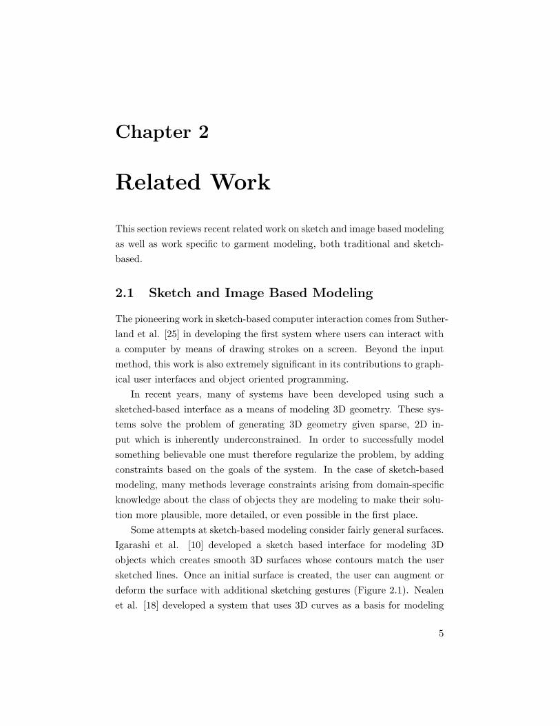
Some attempts at sketch-based modeling consider fairly general surfaces.Igarashi et al. [10] developed a sketch based interface for modeling 3Dobjects which creates smooth 3D surfaces whose contours match the usersketched lines. Once an initial surface is created, the user can augment ordeform the surface with additional sketching gestures (Figure 2.1). Nealenet al. [18] developed a system that uses 3D curves as a basis for modeling

5

2.1. Sketch and Image Based Modeling

Figure 2.1: A user interactively modeling with Teddy[10] (left) by sketching2D strokes while the system generates 3D geometry. This intuitive andeffective means of 3D modeling for novice users was very successful andbecame the basis for commercial applications and video games (right).

operations to allow the user to add fine details to their original model. Inthe case of these systems, only the first curve generates 3D geometry froma 2D input from scratch. The generated surface is typically an amorphous-looking smooth, round shape. After that, additional curves are interpretedin 3D as editing operations with respect to the model in progress. Withenough curves, users are able to model fairly detailed 3D geometry in only afew minutes without prior knowledge of commercial 3D modeling software.These works can be classified as interactive modeling systems, because theyrequire a user to iteratively manipulate the model as the system updatesthe results after each stroke.

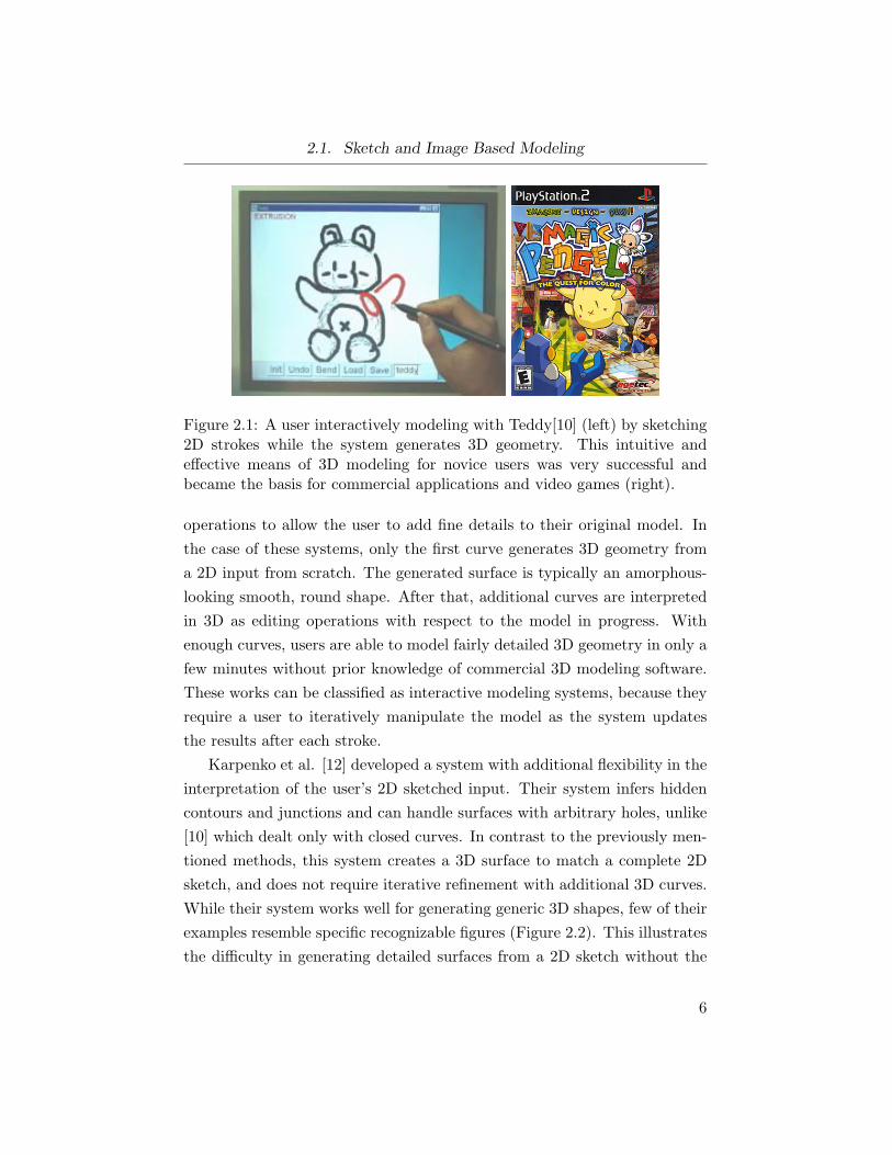
Karpenko et al. [12] developed a system with additional flexibility in theinterpretation of the user’s 2D sketched input. Their system infers hiddencontours and junctions and can handle surfaces with arbitrary holes, unlike[10] which dealt only with closed curves. In contrast to the previously men-tioned methods, this system creates a 3D surface to match a complete 2Dsketch, and does not require iterative refinement with additional 3D curves.While their system works well for generating generic 3D shapes, few of theirexamples resemble specific recognizable figures (Figure 2.2). This illustratesthe difficulty in generating detailed surfaces from a 2D sketch without the

6


Figure 2.2: Two views of three different models generated from Karpenkoet al.[12]. Their system makes no assumptions about the type of objectsthe user wishes to model. As a result, there is limited detail and shapecomplexity that can be achieved in their system.

aid of domain-specific knowledge. The authors hypothesize that more de-tailed results could be generated if the system had a means of predictingthe type of object the user was drawing, perhaps with the aid of a database.This would allow them to maintain a system that did not constrain the userto a specific object domain, but once one is identified it would aid the systemin making interpretations of the user’s sketch.

Bourguignon et al.[3] created a 3D sketching system with multiple ap-plications. The user navigates a 3D scene and augments it by sketching 2Dstrokes. The system will actively reinterpret the stroke’s shape and visibilityas the viewpoint is altered, essentially extending them into 3D. The processinfers a 3D surface for each 2D stroke and migrates the stroke along thissurface as the viewpoint changes. With this framework, they present waysto annotate preexisting 3D scenes, or sketch 3D characters and garmentsby adding strokes from multiple viewpoints. It is important to note thatno actual 3D surface geometry is created with this method, but rather itgenerates viewpoint-adapting 3D lines with some artistic shading to conveythe appearance of a 3D shape.

Many other sketch-based modeling techniques target a specific class ofobjects from the outset and leverage common attributes and principals asso-

7


ciated with members of that class. For many of these techniques the input istoo sparse to generate a perfect 3D representation of the object to be mod-eled, but rather the goal is to create a realistic, believable interpretation ofthe input [21, 22]. For instance, sketch-based modeling solutions to virtualgarments leverage key geometric properties of garments, usually utilizingknowledge about how garments are worn by people [27]. This allows thesesystems to interpret sketched lines differently depending on their orientationand proximity to a mannequin.

Other subject domains have been explored as the basis of 3D modelgeneration [20]. For instance, Fu et al. [5] took a series of sparse, sketchedlines from a user and generated virtual hairstyles. The user only needs todraw lines characteristic of the flow of a hairstyle and the system solvesfor a vector field to fill in regions between user strokes to create a dense,believable hair model.

Mori et al. [16] developed a sketch-based system to create stuffed ani-mals. This method utilize the fact that stuffed animals tend to be smooth,and not contain sharp details like cusps and creases. They maintain a flatpattern that would be used to physically construct the stuffed toy as theuser interactively models the 3D representation. This allows them to con-strain the deformation or augmentation of the model based on the physicallimitations of the pattern.

The system developed in Yang et al. [31] allows for an arbitrary objectclass template to be created and used to model a variety of objects. Theyprovide an algorithm for processing and matching sketched strokes to thisnew object template. This template consisst of one or more definitions of avariety of parts and each user stroke is associated with the best matchingpart. Completing each template is a series of procedural modeling rules forinterpreting the strokes to create a 3D model. They demonstrate templatesfor modeling mugs, planes, and fish. While developing a complete templatewith its associated modeling process may be outside the scope of noviceuser ability, this system could be used by application developers to providetheir users with a sketch-based modeling system for objects relevant to theirsoftware. The example they give would be allowing users to design airplanes

8

2.2. Garment Modeling

for a flight simulator.Architecture is another domain with key principles utilized by sketch-

based geometry generation techniques [17]. Google’s SketchUp [6] programprovides a sketch-based interface to model architecture or other usually man-made objects typical of Computer-Aided Design. It utilizes a method ofinterpreting the implied depth of the user’s object from their 2D sketch.

Image and video based techniques have also targeted specific subject do-mains to generate believable 3D models. Quan et al. [22] utilized knownproperties of plants to do plant reconstruction from multiple images. Forexample, observations about the similarity among leaves aid them in con-structing a generic leaf model that allows for higher quality results in theface of noise or occlusions in the input images. This leads them to createvery believable, realistic looking plants even if they are not able to perfectlyreconstruct the areas hidden from view.

Imaged based architectural modeling systems, like their sketch basedcounterparts discussed earlier, use similar domain-specific attributes of manmade structures to make their modeling problems tractable. Most structuresare built of mostly planar, often symmetrical, smooth surfaces and knowingthis makes interpreting images and user drawn sketches much easier andmore accurate. Sinha et al. [24] are able to detect planar surfaces andcamera properties from photographs to reconstruct buildings and rooms.

2.2 Garment Modeling

2.2.1 Traditional Garment Modeling

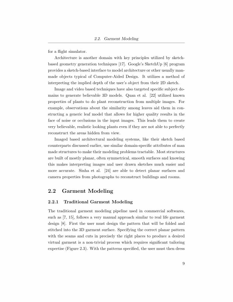
The traditional garment modeling pipeline used in commercial softwares,such as [7, 15], follows a very manual approach similar to real life garmentdesign [8]. First the user must design the pattern that will be folded andstitched into the 3D garment surface. Specifying the correct planar patternwith the seams and cuts in precisely the right places to produce a desiredvirtual garment is a non-trivial process which requires significant tailoringexpertise (Figure 2.3). With the patterns specified, the user must then dress

9


Figure 2.3: An example of modeling a shirt with MayaCloth[15]. The properplacement of seams and cuts in the shirt pattern is critical to generating aplausible virtual garment and is not an quick or intuitive process for noviceusers.

the mannequin, which requires that the patterns be tuned to the proportionsand scale of the mannequin. To make the dressed mannequin appear natural,users typically run a physical simulation to account for gravity and collisions.The simulation often requires a significant amount of trial-and-error-basedparameter tuning to obtain a desired look. Despite recent advances [9],simulation interfaces remain challenging to use for non-experts. The entireprocess is extremely labour intensive and difficult to master. It requiresworking knowledge in three otherwise disjoint fields: tailoring, artistic useof 3D modeling programs, and specifying and tuning physical simulations.

Consequently, numerous attempts were made to simplify the modelingprocess. Wang et al. [30] propose creating templates of clothing componentsand defining rules on how these templates fit together to create completegarments. This approach allows the user to mix and match components togenerate new garment forms, assuming the desired components are alreadyavailable, which is often not the case. Others [4, 23, 27, 28] propose usingsketch-based methods for garment modeling as discussed next.

2.2.2 Sketch-Based Garment Modeling

The motivation for a sketch-based system for modeling virtual garmentsstems directly from the complexities of using a traditional garment modelingsystem for non-expert users. Novice users may have a vivid idea of the shape

10


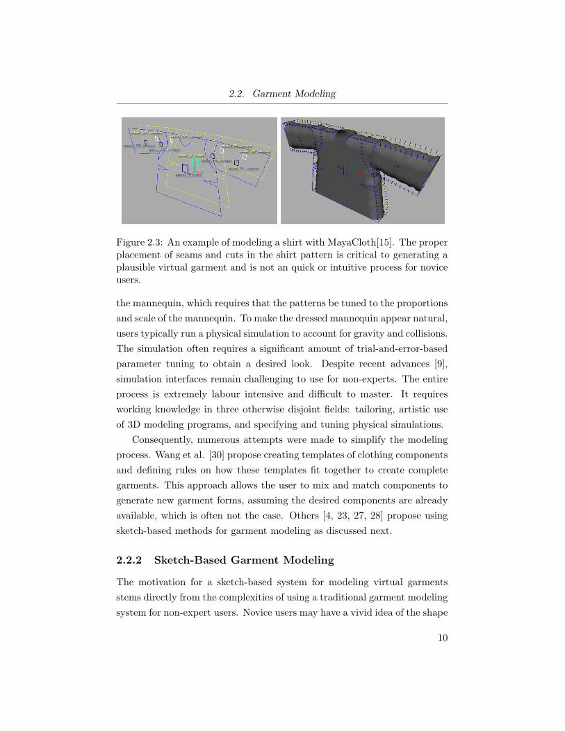
Figure 2.4: An example from Turquin et al.[27]. In contrast to the com-plexities of traditional virtual garment design, this system allows the userto simply draw the outline of a shirt and the system generates a 3D surfacethat satisfies the user’s sketch.

of the virtual garment they wish to model, but at no point in the traditionalgarment modeling pipeline do they get to directly specify the shape of adesired end-product. Furthermore, if they manage to run the whole pipelineand the resulting garment is not quite what they had desired, it may not beobvious how to modify the planar patterns to correct the final result.

Inspired by the difficulty of traditional virtual garment design, Turquinet al. [27] introduce a sketch based system for garment modeling drasticallysimplifying the process, specifically making the user input much more intu-itive. Now, the user is allowed to simply draw a 2D outline of the garmentthey wish to model, and from it the system generates a 3D virtual garment.The user is given a virtual canvas with a 3D mannequin, and proceeds todress the mannequin by drawing lines on the canvas. The drawn lines are in-terpreted as one of two different categories. The first being silhouettes, whichthe user is specifying where the desired 3D garment is wrapping around themannequin to the backside. The second type of lines are garment borders,like the neckline or hem of a dress. The classification of these lines becomesas simple as identifying which lines cross the mannequins body (borders)and which lines do not (silhouettes). Once the system has classified theinput lines, it proceeds to generate a 3D surface. An observation made by

11


Figure 2.5: An example result from Turquin et al. [27]. Notice how thesurface widens at the bottom (red box) of the dress as if it were following themannequins leg shape, even though it is too far away from the mannequinto be expected to do so. This is because their offset surface method takesmannequin shape into account even in loose regions, leading to results nottypical of real world garments.

Turquin et al. is that given a garment sketch the viewers would expect thedistance from the garment to the mannequin body to be mostly consistentas we move in the direction across the body, perpendicular to the torsoand limbs. Since the distance from the silhouette lines to the body can bemeasured, they utilize it to create an offset surface representing the virtualgarment. An offset surface is a surface defined at each point by a value thatspecifies the distance from the surface to the mannequin. This distance-to-body value is measured for each of the silhouette lines and interpolated foreach of the border lines. These distance-to-body values are then propagatedto the surface interior. Additional calculations are done to simulate clothtension, specifically in regions between limbs.

The resulting virtual garments are indeed consistent with the user’s inputsketch from the front view, however the use of an offset surface has its ownundesirable effects. Most notably, the depth of loose areas of the garmentare influenced by the mannequin shape underneath, even when the garment

12


Figure 2.6: In the system developed in [28], the user sketches additionallines besides the outline to produce more detailed results. In this case,the user sketches vertical strokes (green) to model folds and wavy strokes(purple) to indicate a wavy border at the bottom of the skirt.

is significantly far away from the mannequin where the viewer does notexpect the mannequin to have a direct influence on the garment shape. Forinstance, in Figure 2.5 the surface at the bottom of the skirt (red box) jutsoutward because of the mannequin’s leg shape. This looks unrealistic andthe system does not have a way for the user to correct such behavior oncethe surface is generated. Such unintuitive influence of the mannequin bodyin loose regions is only magnified on extremely loose garments.

This work is extended in Turquin et al. [28] to include additional typesof input lines that could model more complicated garment behavior. Figure2.6 shows how the user can draw lines to specify a wavy border and folds.The more of these new features that are added to the sketch-based system,the more complicated the sketching gesture language becomes. The originalmotivation for a sketch-based interface is to allow the user to easily draw a2D representation of the 3D surface they wish to create. The more compli-cated that process becomes, the more time and effort the user must spendto learn how to use the modeling interface. As a result, these methods havea trade-off between ease of input and quality of results.

Other works [4, 23] have focused on utilizing surface developability to

13


model more realistic garments with a sketch-based interface. Mathemati-cally, a surface is developable if it has zero Gaussian curvature. In laymen’sterms, any surface that can be laid into a flat plane with no distortion isdevelopable. Real-life garments are quasi-developable because their pat-terns consist of planar pieces. Once constructed, real-life garment materialsoften exhibit little stretch or distortion from their original pattern shape,so they largely continue to behave like a developable surface. Decaudin etal. [4] augment the sketching system from [27] by taking the resulting sur-face and deforming it to increase its developability. Then they procedurallymodel fabric buckling to create realistic folds. Rose et al. [23] replace thedistance-based surface within each panel by a developable approximation.Both methods continue to use the distance to body metaphor to infer theseam positions and the results rely heavily on the quality and placement ofthe seams.

Our method improves on the surface modeling approach proposed bythese works in two ways. First, we produce a more realistic-looking in-terpretation of the input, especially in loose, interior regions. Second, weprovide a much more intuitive method of input, allowing the user to drawor provide a previously drawn image of the front view of a person wearingthe garments they wish to model. Unlike previous sketch-based methods,the user is not limited to a mannequin provided by the sketching canvas,and they do not need to learn a sketching gesture language to communicatewith the system.

14

Chapter 3

Virtual Garment Modeling

3.1 Overview

The goal of our system is to create realistic-looking garment models fromfashion drawings or sketches using similar cues to those used by humanswhen interpreting such drawings. As already observed by Turquin et al.[27] the human interpretation of a drawn garment is strongly linked to theshape of the garment wearer. When modeling a garment from a fashiondrawing, in contrast to the sketching setup of Turquin et al., we do not apriori have a model of the wearer. We observe that typical fashion drawingscontain the entire dressed figure [1, 11] as, predictably, it helps the viewerto interpret the garment proportions. We therefore use this drawn figure tofit a 3D human template or mannequin to the drawing (Section 3.2). Ourfitting process starts by fitting a planar skeleton model (Figure 3.1) to thedrawing, extracting the mannequin’s pose and proportions and then refiningthe fit using the actual mannequin. We combine the fitting process with ananalysis of the drawing that identifies characteristic garment lines that aresubsequently used by the modeling process (Figure 3.1). Given the set oflines and the fitted mannequin we proceed to model the actual garment. Themodeling process is one of the key contributions of this work The methodis based on a new interpretation of the characteristic lines, leading to thecreation of more realistic-looking garments than previous techniques.

3.2 Drawing Analysis

The drawing analysis performs two tasks necessary for the garment modelingstage: it fits a mannequin to the drawn figure and identifies the characteristic

15

3.2. Drawing Analysis

(a) (b) (c)

(d) (e) (f)

Figure 3.1: Fitting and line analysis for a garment in Figure 4.4: (Leftto right) skeleton in rest pose with typical female figure proportions; initialregions and outline; skeleton fit to initial outline; clustered regions and up-dated outline (extremity clusters, removed later on, shown in grey); skeletonfit to new outline; characteristic line labeling with silhouettes in red, bordersin green and part boundaries in yellow.

garment lines in the drawing. We assume that the drawings are purely line-based or, alternatively, that the lines had been extracted from the drawingusing standard image-processing software. As a pre-processing step we closesmall gaps in the line drawing, extending existing lines along the tangentdirection by an epsilon distance if the extension reaches another line, andextract all the connected regions (Figure 3.1 (b)). We define the initialoutline of the drawn figure as the boundary of the outer region and useit to perform initial mannequin fitting (Section 3.2.1). We then perform

16


further analysis on the drawing using the obtained mannequin fit to detectany interior loops as well as inner silhouette edges (Section 3.2.2) and usethose to refine the fit (Figure 3.1 (e)). The result of the final fitting is usedto identify and label the characteristic garment lines (Section 3.2.2).

3.2.1 Mannequin Fitting

The implementation for this section was originally programmed by VladislavKraevoy, and is included here for the sake of completion. Since its originalimplementation, both the skeleton fitting and mannequin refinement processhas been expanded upon and maintained by Cody Robson.

Our method fits a rigged human template or mannequin to the outline ofa dressed figure. This task is quite similar to the fitting of human templatesto segmented images [2, 29]. In general, due to the vast variety of humanposes, such fitting is quite challenging, with the methods above relying onimages taken from multiple views to extract the template’s pose and pro-portions. In our case, only one view is available. However we can rely ona number of assumptions about typical character poses and view directionsused in the fashion drawings to simplify the problem. Specifically we ob-serve that the subjects nearly always face the viewer and are typically drawnin a standing pose with articulation largely limited to the image plane, assuch poses tend to best showcase the garment [11]. Thus we can effectivelyreduce the pose-extraction component of the fitting to two dimensions, ori-enting the mannequin to face the viewer and restricting the articulation tothe image plane.

Following [29] we use a two-step fitting approach. We first fit a 2Dskeleton structure to the outline, obtaining the pose and proportions usedto adjust the mannequin rig and to skin it, and then fine-tune the fit usingthe actual mannequin.

Skeleton Fitting: We associate a skeleton with a basic set of links(Figure 3.1(a)) with our mannequin. Each link is defined as a rectanglewith associated width and length and a specified connectivity to other links.In contrast to Vlasic et al. we do not know a priori the proportions of

17


the drawn figure and thus cannot specify the link dimensions beforehand.Instead, to maintain realism, we rely on human proportion ratios typicallyused in fashion drawings [1, 11], for instance requiring thighs and calves tobe the same length.

The skeleton fitting is performed using non-linear optimization with thelink dimensions and joint angles as unknowns and is based on the followingset of considerations.

• We clearly expect the mannequin to be bounded by the outline of thedressed figure and thus expect the skeleton to be contained by it. Toreflect this expectation, our non-linear optimization function containsa term measuring an asymmetric signed distance from the sides of theskeleton links to the outline. The distance is measured by sampling thelink sides at equal intervals and computing the signed distance from thesampled points to the closest points on the outline. The metric becomeszero if the distance is negative.

• Since garments in general can be quite loose, we do not expect the skele-ton to closely match the outline. However, we can expect the sides ofthe links to be close to the outline in the parts of the skeleton wherethe drawing typically shows the actual wearer’s body, such as wrists andankles, and along the shoulders where gravity dictates a tight garmentfit. The optimization term reflecting this expectation measures the dis-tance from these points on the skeleton links to the closest point on theoutline, where we take the distance into account only if the relevant skele-ton points are inside the outline. This term is necessary to prevent themannequin from “floating inside” the drawn figure.

• For the same reason we use an anti-shrinkage term which pulls the man-nequin head toward the top of the outline and the feet toward the bottom.

• We add a term aiming to maintain the typical proportion ratios [1] be-tween link dimensions.

• Most figures in fashion drawings have fairly simple poses, as those best

18


showcase the actual garment. Hence the optimization includes a termaiming to preserve the skeleton angles relative to a default rest pose.

We initiate the skeleton fitting by aligning the skeleton with the centerof mass of the outline and scaling it to fit the outline height. To speedup convergence, as an initial guess we place arm and leg joints as muchapart as the outline allows, while keeping the torso centered at the midpointbetween them. We use the line-search method as implemented in Matlabto solve for the optimal skeleton placement. The distances in all the termsare normalized with respect to outline height. The term weights are one,one, eight, five and one hundred, respectively. The high weight for angledeviation is the result of differences in scale between distances and angles.The fitting is first performed with the initial outline and then refined usingthe more detailed outline computed as described in Section 3.2.2.

Local Mannequin Deformation: Once the skeleton fitting converges,we fit the actual mannequin to the drawing. We pose the mannequin andadjust its proportions based on the skeleton fitting results, using standardskinning techniques. Following the fitting the mannequin captures the over-all shape of the dressed figure, however minor local misalignments may stillexist. Most are harmless from the garment modeling point of view. However,parts of the mannequin may protrude outside the outline, causing potentialartifacts in the subsequent modeling stage.

To improve the fit we compute matches between the outline and themannequin and use those to deform the mannequin toward the outline,using linear Laplacian deformation [13]. For each point on the outline wefind the best-fitting mannequin point using a combination of normal andposition similarity,

‖p− v‖2 + ψ(np · nv − 1)2

where p and v are the 2D positions of the matched points and np and nv

the respective 3D normals. We set ψ = 100 in all examples. The useof the normal component is critical to ensure that only points on or closeto the mannequin silhouette are considered by the matching. We ignorematches where the mannequin point is already inside the outline as well

19


as outlier matches. To resolve inconsistent matches we use an ICP-likesetting treating matches as soft constraints, and repeating the match-and-deform steps several times with increasing constraint weight. The processis repeated until the mannequin lies entirely inside the outline.

3.2.2 Line Analysis and Labeling

The analysis has three main goals: extracting and labeling characteristiclines, identifying non-garment drawing elements (extremities), and refiningthe outline. Since we assume the drawing contains a full human figure weexpect the extremities (hands, feet, head) to show up in most drawings.However, we do not expect them to correspond to actual outfit parts (wedo not aim to model gloves, shoes, or hats). Thus we detect the extremitiesand remove them from the modeling input.

Separating Body Parts: We roughly identify the major body partsof the drawn dressed figure, associating regions in the drawing with groupsof skeleton links representing body parts significant for modeling purposes(Figure 3.1 (d)) and clustering them together. Thus, shoulders and uppertorso, thighs and lower torso, and head and neck are each viewed as onegroup. The association is loosely based on the amount of overlap in theplane between the regions and the link groups representing each part.

To initiate the extremity detection process, for each of the extremitygroups we locate the biggest region overlapping it and associate the regionwith it. We then associate the remaining regions with the parts they over-lap most, initially leaving regions that do not overlap the skeletal links oroverlap only a small portion of a link (less than 30% of the region area)unassigned. For regions that overlap multiple body parts, such assignmentmay not be best. To improve assignment we perform re-clustering based oncluster compactness. Regions are moved from one cluster to another if theyoverlap the links associated with both and the reassignment shortens thesum of cluster perimeters. The re-clustering ignores the regions assigned toextremities in the first stage. Finally we process the previously unassignedregions, testing if they can correspond to interior outline loops. We check

20


if they are surrounded by assigned regions and if the shared boundariesare aligned with the corresponding skeleton links. If the answer is yes, theregions are classified as exterior and their boundary is added to the out-line. Otherwise they are added to the best-fitting adjacent cluster based oncompactness. Pseudocode for this algorithm is shown in 3.2.

The results of the clustering are used to refine the skeleton fit and tofacilitate line labeling. Following the fitting, the clustering is performedagain to capture minor changes in skeleton layout.

Line Labeling: The labeling step extracts from the drawing the fourtypes of lines: silhouettes, borders, part boundaries, and folds (Section 3.3)used by our garment modeling algorithm. Following the clustering stage weexpect the cluster boundaries to capture the lines in the drawing that fit inone of the first three categories.

We begin by considering the boundaries between adjacent clusters. Byconstruction the boundaries consist of polylines that are either aligned withcorresponding skeleton links or perpendicular to them. Polylines alignedwith the links are likely to be model silhouettes that separate body parts,e.g., the torso from the arms or the legs from one another. The perpendicularpolylines are likely to be borders or part boundaries. To extract the twotypes of polylines we process each boundary edge independently, labelingit as silhouette or part boundary based on the angle between it and thecorresponding links. We found this simple procedure to produce correctlabeling. The identified silhouettes are treated as duplicate outline edges bythe fitting and modeling stages. The part boundary labeling is temporaryand can be changed later on.

We now proceed to label the outlines. Outline edges can belong to one oftwo categories, silhouettes or borders. We expect silhouettes to be alignedwith the skeleton, and borders to be roughly perpendicular to it. Howeverin this case edge level labels can be inaccurate. To obtain a conclusivelabeling we employ a bottom up clustering with the expectation that anoutline should be split into only a few border or silhouette edge sequences.First each outline edge is labeled independently using two criteria: the anglebetween the edge and the closest skeleton link, and if the edge shares a vertex

21


// find the extremitiesfor all bone ∈ E do

bestArea← 0;bestRegion← Null;for all region ∈ R do

overlap← AreaIntersection(region, bone);if overlap > bestArea then

bestArea← overlap;bestRegion← region;

end ifend forregionBones[bestRegion]← bone;regionClusters[bestRegion]← boneCluster[bone];

end for// assign bones for remaining regionsfor all region ∈ R do

if regionClusters[region] 6= Null thencontinue;

end ifbestArea← 0;bestBone← Null;for all bone ∈ B do

overlap← AreaIntersection(region, bone);if overlap/Area(region) > .3 and overlap > bestArea then

bestArea = overlap;bestBone = bone;

end ifend forregionBones[region]← bestBone;regionClusters[region]← boneCluster[bestBone];

end for// test compactnessfor all cluster ∈ C do

myParimeter ← Parimeter(cluster);for all nregion ∈ GetNeighborRegions(C) do

newParimeter ← Parimeter(cluster + nregion);if newParimeter < myParimeter then

regionClusters[nregion]← cluster;end if

end forend for// process unassignedfor all region ∈ R do

if regionClusters[region] 6= Null thencontinue;

end ifbestParimeter ← 0;bestCluster ← Null;for all nregion ∈ GetNeighborRegions(region) do

if regionClusters[nregion] == Null ornot IsAligned(Border(region, nregion), regionBones[nregion]) then

bestCluster ← Null;break;

end ifmyParimeter = Parimeter(regionClusters[nregion] + region);if myParimeter < bestParimeter or bestCluster == Null then

bestParimeter ← myParimeter;bestCluster ← regionClusters[nregion];

end ifend forregionClusters[region]← bestCluster;

end for

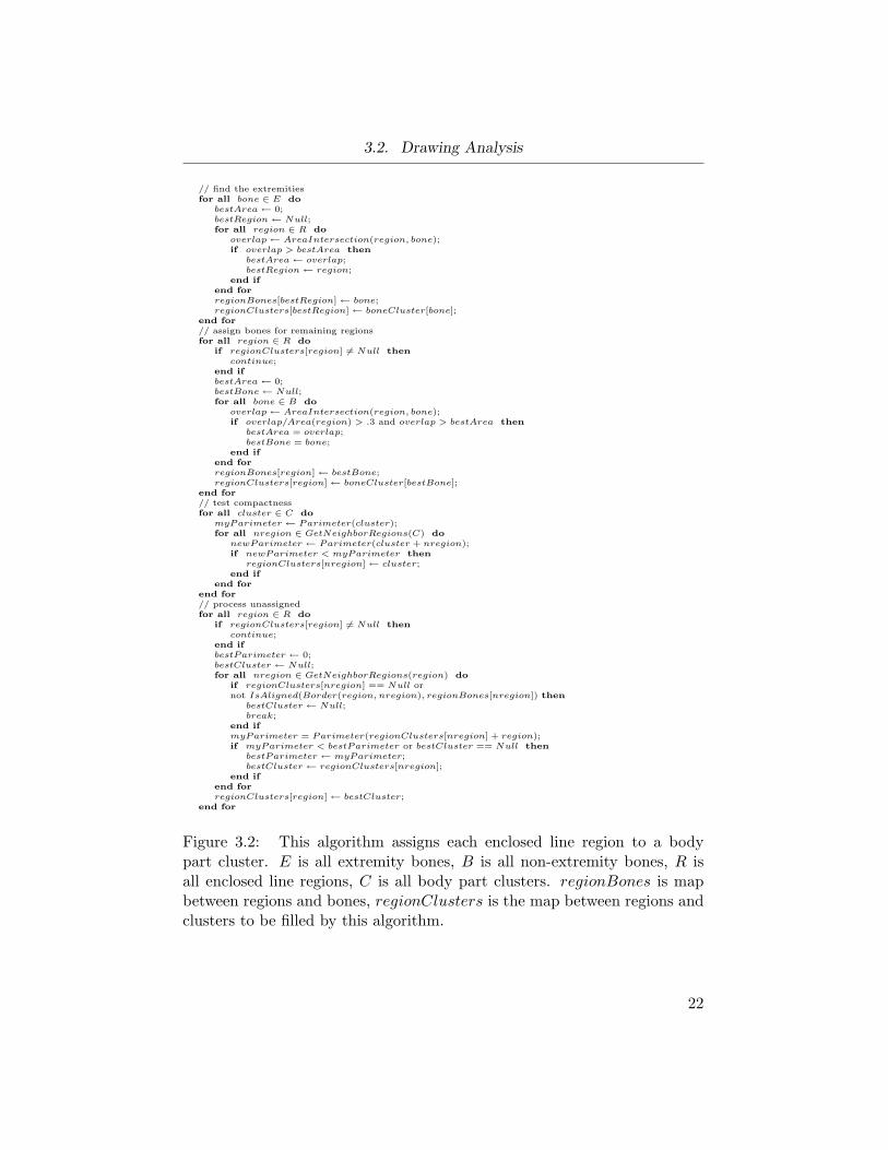
Figure 3.2: This algorithm assigns each enclosed line region to a bodypart cluster. E is all extremity bones, B is all non-extremity bones, R isall enclosed line regions, C is all body part clusters. regionBones is mapbetween regions and bones, regionClusters is the map between regions andclusters to be filled by this algorithm.

22

3.3. Garment Surface Modeling

with a line classified as part boundary in the previous stage, the angle withthis line. The classification error for an edge labeled as silhouette is measuredas 6 (e, s)2 + (π/2− 6 (e, b))2) where e is the edge in question, s the skeletonand b the adjacent part boundary. If no adjacent part boundaries exist, onlythe first term is used. The error effectively measures how far the edge is frombeing parallel to the skeleton and perpendicular to the part boundary. Theclassification error for an outline edge labeled as border is effectively invertedand is measured as (π/2 − 6 (e, s))2 + 6 (e, b)2). We first label each edgeindependently, selecting the label with smaller error and then incrementallyinvert the labeling of sequences of edges. We stop once the next label fliprequires an order of magnitude jump in the error (in all our experimentsthis was an ideal indicator of overclustering). Once the process terminates,part boundaries adjacent to borders and aligned with them are relabeled asborders. Region boundaries interior to clusters but aligned with the newlyidentified border lines are similarly labeled as borders. Finally, we discardthe detected extremity clusters relabeling part boundaries adjacent to themas borders and identify folds, as relatively straight lines in the drawing thatgo upward from borders.

User Interaction: The analysis step is based on a number of assump-tions about garment drawings, which while holding true for most models,can break up in some setups. Both part identification and line labeling errorscan be trivially corrected by the user via a basic visual interface. Once theidentification or labeling are corrected the rest of the algorithm can proceedas is. Chapter 4 discusses the type of inputs where this mechanism mightbe utilized.

3.3 Garment Surface Modeling

Our modeling algorithm generates three-dimensional realistic-looking gar-ment surfaces using as input the posed mannequin on which we fit the gar-ment and a labeled set of characteristic lines describing the garment. In thiscontext, we associate a local body-aligned frame with each surface vertex,where body-aligned refers to alignment with the corresponding link in the

23


Figure 3.3: Modeling stages for the suit in Figure 1.1: (top) posed man-nequin and labeled lines, wrapper surface, (bottom) tightness mask andfinal surface.

24


mannequin skeleton. The frame consists of a body-aligned vector and twocross-body vectors orthogonal to it, one of which is in the image plane. Sofor example on a sleeve we will have one vector aligned with the arm link orbone and two perpendicular to it.

3.3.1 Line Interpretation

For modeling purposes we use four types of lines, extracted by the draw-ing analysis: silhouettes, borders, folds, and part boundaries (Figure 3.3, topleft). The silhouettes represent the locations where the back and front gar-ment surfaces coincide. The borders correspond to depth discontinuities inthe outfit, indicating garment boundaries. Folds capture interior silhouetteson the front of the garment where the surface normal is roughly orthogonalto the viewer. Part boundaries correspond to natural boundaries betweenmajor body parts(e.g. between the upper and lower torso or between theshoulder and upper arm) present in the drawing and extracted by our lineanalysis algorithm, effectively as a by-product. The modeling process isbased on number of observations or assumptions about human interpreta-tion of these types of lines in fashion drawings.

Silhouettes: The silhouettes undoubtedly provide the strongest cuesto the 3D shape of the garment. However, the question of how to interpretthem remains open. Instead of the offset-based interpretation [27], we spec-ulate that the human interpretation of silhouettes takes into account threepotentially conflicting factors: the silhouette shape, avoidance of garment-body intersections, and lastly gravity. We speculate that when silhouettesare far from the body their shape dictates much of the garment shape.Specifically, the normals along silhouettes seem to predict the body-alignedcomponent of the surface normal across the body, and to a lesser degree theother normal components. The silhouette influence on the normal is sub-ject to some attenuation the further we are from the silhouettes due to thefact that garments often have side seams, the stiffness of which counteractsgravity while in typically seamless areas, on the back and front, gravity islikely to play a bigger role, reducing the vertical component of the surface

25


normal. In regions where the silhouettes are close to the body, avoidanceof garment-body intersections leads to the expectation of garments tightlywrapping the body, overriding other considerations.

Borders: In traditional fashion drawings the viewer is assumed to bestanding at a finite distance from the drawn figure and at the same eyelevel. This assumption combined with the expectation of garment bordersto be roughly planar produces a subtle visual effect heavily utilized in fash-ion drawings that often lets viewers infer the depth profile along garmentborders (Figure 3.4). Given the shape of the border, viewers appear touse it to infer the cross-body profile of the garment near the border. Inother words, the cross-body components of the vertex normals at the bor-der strongly influence the cross-body normal components along the surface.Thus, combining the silhouettes and the borders effectively provides the nor-mals across the surface in loose garment regions, defining the surface shape.As demonstrated by the figures throughout this paper, this interpretationappears to lead to realistic-looking results consistent with the drawings.

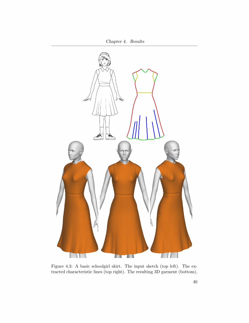
Folds and Part Boundaries: Fashion drawing often contain multipleother lines in addition to silhouettes and borders. Many of those reflecttexture and not geometric details. Others capture details that are not front-back symmetric, namely ones showing on the front but not on the back,such as pockets or collars. We focus on modeling garment geometry anduse the drawing to infer the back geometry as well. Thus we only considerlines indicating geometric features that are likely to exhibit a front-backsymmetry. Both folds and part boundaries fit these criteria, with folds hav-ing an obvious geometric meaning and part boundaries typically indicatingthe presence of narrow grooves on the surface usually found at seams ortransitions between garments (Figure 4.3).

As noted earlier the modeling considerations are significantly differentin tight and loose regions of the garments. Hence our modeling procedureoperates in two stages (Figure 3.3), first computing a tight-fitting wrap-per garment that provides a feasible geometry for the regions where thesilhouettes are close to the mannequin (Section 3.3.2), and then updatingthe geometry in loose regions to reflect the additional considerations while

26


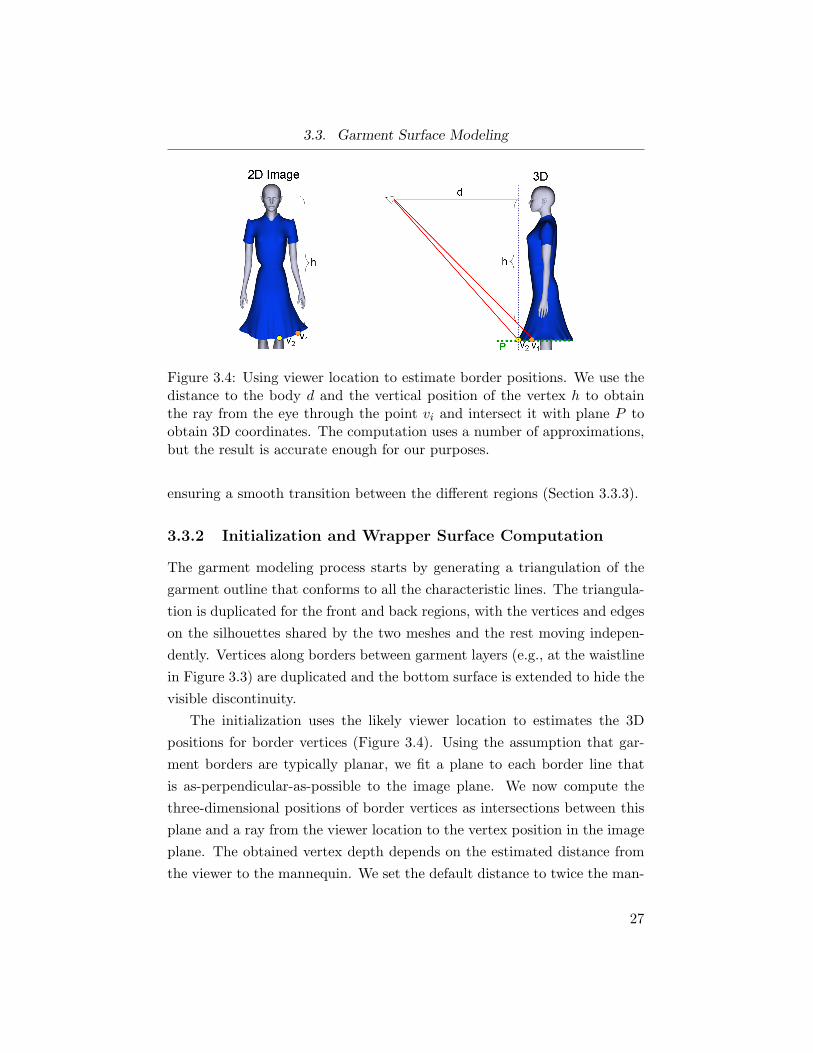
Figure 3.4: Using viewer location to estimate border positions. We use thedistance to the body d and the vertical position of the vertex h to obtainthe ray from the eye through the point vi and intersect it with plane P toobtain 3D coordinates. The computation uses a number of approximations,but the result is accurate enough for our purposes.

ensuring a smooth transition between the different regions (Section 3.3.3).

3.3.2 Initialization and Wrapper Surface Computation

The garment modeling process starts by generating a triangulation of thegarment outline that conforms to all the characteristic lines. The triangula-tion is duplicated for the front and back regions, with the vertices and edgeson the silhouettes shared by the two meshes and the rest moving indepen-dently. Vertices along borders between garment layers (e.g., at the waistlinein Figure 3.3) are duplicated and the bottom surface is extended to hide thevisible discontinuity.

The initialization uses the likely viewer location to estimates the 3Dpositions for border vertices (Figure 3.4). Using the assumption that gar-ment borders are typically planar, we fit a plane to each border line thatis as-perpendicular-as-possible to the image plane. We now compute thethree-dimensional positions of border vertices as intersections between thisplane and a ray from the viewer location to the vertex position in the imageplane. The obtained vertex depth depends on the estimated distance fromthe viewer to the mannequin. We set the default distance to twice the man-

27


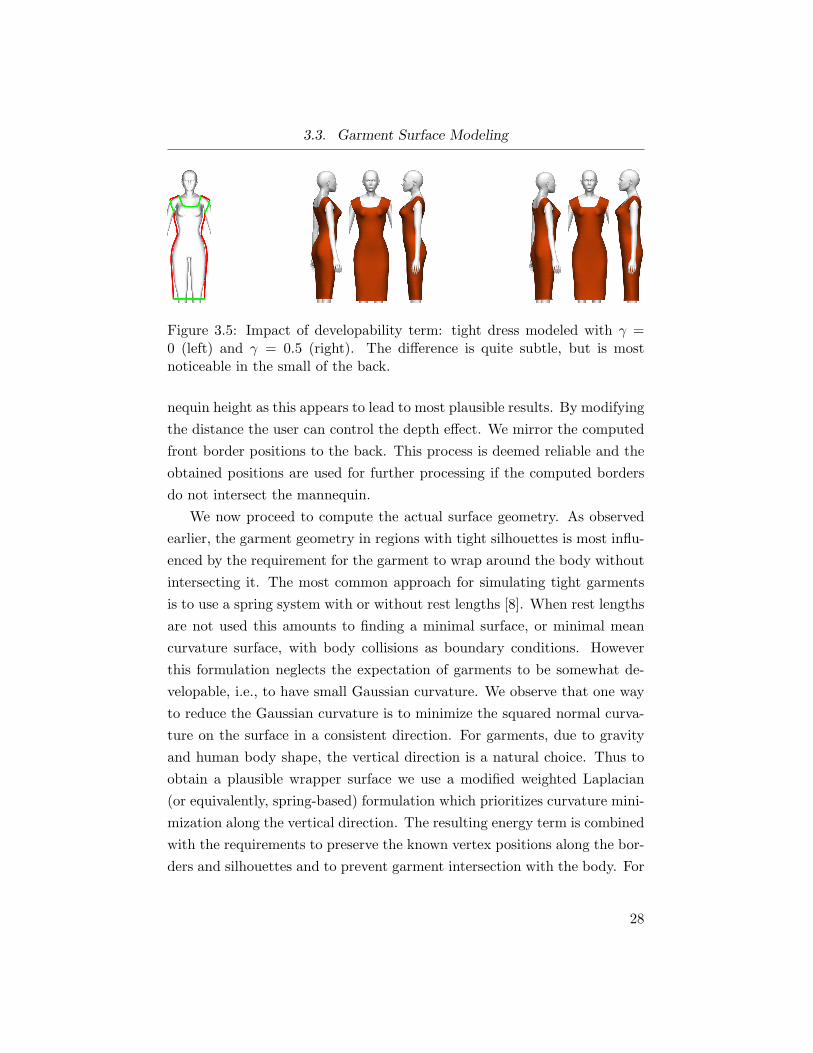
Figure 3.5: Impact of developability term: tight dress modeled with γ =0 (left) and γ = 0.5 (right). The difference is quite subtle, but is mostnoticeable in the small of the back.

nequin height as this appears to lead to most plausible results. By modifyingthe distance the user can control the depth effect. We mirror the computedfront border positions to the back. This process is deemed reliable and theobtained positions are used for further processing if the computed bordersdo not intersect the mannequin.

We now proceed to compute the actual surface geometry. As observedearlier, the garment geometry in regions with tight silhouettes is most influ-enced by the requirement for the garment to wrap around the body withoutintersecting it. The most common approach for simulating tight garmentsis to use a spring system with or without rest lengths [8]. When rest lengthsare not used this amounts to finding a minimal surface, or minimal meancurvature surface, with body collisions as boundary conditions. Howeverthis formulation neglects the expectation of garments to be somewhat de-velopable, i.e., to have small Gaussian curvature. We observe that one wayto reduce the Gaussian curvature is to minimize the squared normal curva-ture on the surface in a consistent direction. For garments, due to gravityand human body shape, the vertical direction is a natural choice. Thus toobtain a plausible wrapper surface we use a modified weighted Laplacian(or equivalently, spring-based) formulation which prioritizes curvature mini-mization along the vertical direction. The resulting energy term is combinedwith the requirements to preserve the known vertex positions along the bor-ders and silhouettes and to prevent garment intersection with the body. For

28


the silhouettes we only preserve the positions in the image plane, letting thevertices move freely in the depth coordinate. Combining these requirementsyields the following optimization functional:

min∑i

‖vi −1∑

(i,j) φij

∑(i,j)

φijvj‖2 +

δ∑i∈S

[(vxi − cxi )2 + (vyi − cyi )

2] + δ∑i∈B‖vi − ci‖2 (3.1)

where vi are the mesh vertices, S and B are the sets of silhouette and bordervertices respectively, φij = (1− γ) + γe((1−Nij ·V )/σ1)2 , Nij is the direction ofvivj and V the vertical direction. We set δ = 100, σ1 = 0.1 and γ = .5 inall our examples. The choice of soft rather than hard constraints creates asmoother and more natural surface shape near the constrained vertices. Theintersection avoidance is incorporated explicitly through the use of a Gauss-Seidel type solver. The process is initiated by moving each interior vertexof the mesh along the depth axis to avoid intersection with the mannequin.At each iteration, if the new position, computed based on Equation 3.1, isinside the mannequin, the vertex is only moved along the vector between theold and new positions until it lies on the mannequin surface. An exampleresult demonstrating the impact of the vertical weighing is shown in Figure3.5. The main difference is in the amount of garment “stickiness” in concaveregions, such as the small of the back, where using γ > 0 we achieve resultsmore consistent with less stretchy fabrics and a lack of tightly-tailored seams.

During the iterations, determining if a candidate position lies inside themannequin can be expensive if not done properly. In the naıve case, wewould need to calculate the distance from each vertex’s candidate positionto each triangle on the mannequin mesh, taking a prohibitively long time.To make the process efficient we utilize a pre-computed distance transformfunction. A distance transform function computes the distance to a givenmesh for each point on a regular grid. Once computed, it provides fastdistance estimates for any arbitrary point in the space spanned by the grid.To estimate the distance from a candidate vertex position to the mannequinmesh, we simply take a weighted average of the eight nearest grid points’

29


distance values. Accessing a regular grid and trilinearly interpolating eightdistance values is much faster than computing distances on the fly, andprovides a satisfactory distance estimate for our purposes. We utilized animplementation of the distance transform introduced in [14], which has linearcomplexity both in the number of grid points and the size of the mesh.

3.3.3 Modeling Complete Garments

For a tight-fitting outfit the wrapper provides a feasible interpretation. How-ever for outfits that have loose regions we need to incorporate additional in-formation into the setting, specifically the shape of the silhouettes, bordersand folds. We do this using a normal based surface editing approach, asenforcing normals implicitly enforces the shape of a surface.

Tightness Mask

We start by computing a tightness mask, which for each vertex indicateshow much we expect the wrapper surface solution to be preserved locally.The mask is set to zero or near zero in loose regions and is close to onein tight regions (Figure 3.3). We first compute the value of the tightnessmask along the silhouettes and then propagate it inward. The mask at thesilhouette vertices is a function of the planar distance d, from the vertex tothe body (normalized with respect to the mannequin bounding box), and isset using a Gaussian distribution to e(−d/σ2)2 with a value of σ2 = 0.003, aswe want the mask to become zero once we move away from the mannequineven slightly.

To distribute the values across the mesh we solve a least-squares mini-mization, which assigns similar mask values to adjacent vertices. Since weexpect the fit distance to remain roughly similar as we circle around themannequin, we assign higher weights to pairs of vertices locally aligned withthe 2D cross-body direction.

min∑ij

wij(mi −mj)2 subj to mi = Mi, ∀i ∈ S

30


where mi are the per vertex masks and Mi are the masks computed for the

silhouettes vertices. The weights wij are set to 1/‖vi − vj‖e−|Nij ·(Li+Lj)/2|

σ3

2

,where Li is the direction of the skeleton link associated with vi. To betterpropagate mask values across the body, the sum

∑ij includes a two-ring

neighborhood of each vertex. Based on experiments we set σ3 = .5. Wesolve the resulting linear system using Cholmod [26].

Solving for Normals

We expect the general garment shape in loose regions to be determined bythe normals along the silhouettes and borders. To this effect we propagateboth types of normals across the body. To incorporate the observationsabout the asymmetric impact of the border and silhouette normals on thetarget surface we separate the body aligned and cross-body components inthe computation.

To initialize the computation we fix the normals at silhouette vertices totheir image plane values. If the border vertex depth information is deemedreliable by the initialization step, at each border vertex we compute andfix the cross-body normal components. We expect the body-aligned normalcomponent to be most similar as we circle the body, or go across it, and thecross-body components to be more similar in the body-aligned direction. Tothis end we assign appropriate smoothing weights when propagating the two.In addition we introduce an attenuation term on the vertical component ofthe normal to account for gravity. The combined minimized functional is

min∑i

mi(ni − n′i)2 + (1−mi)∑ij

[wij‖nai − naj‖2

+w′ij‖npi − n

pj‖

2] + αnyi2,

where nai is the body-aligned component of the normal, npi is the cross-bodycomponent, and n′i are the initial normals computed on the wrapper surface.The weights wij are the same as for the mask computation, propagating thebody aligned component across the body. The weights w′ij are defined to

31


identically spread the cross-body components along the body. As in themask computation the sum

∑ij includes a two ring neighborhood of each

vertex. We set α = 0.05.We solve this non-linear problem using Gauss-Seidel iterations. Since

the solution involves normals, we need to renormalize them at each iter-ation. However, standard renormalization provides unintuitive results inour setting. Consider two normals at the sides of a cone, propagated alonga circular arc. We would naturally expect the normal component alignedwith the cone axis to remain the same. However, naıve normal averagingcombined with normalization will in fact change it. In our setting whenaveraging normals on opposing silhouettes we have a similar expectation ofthe body-aligned normal component being the average of the correspondingcomponents at the silhouette. We therefore explicitly separate computationfor the body aligned and cross-body components, renormalizing only thecross-body components as necessary to preserve the overall unit length.

Folds: After we compute the basic normals across the surface, we in-corporate folds into the setting as lines along which the normal is rotatedaway from the view direction, perpendicular to the fold axis. Starting atthe bottom of each fold we have the option to use the normal at the bottompoint (recall that by construction the bottom point of each fold lies on aborder) or to turn the normal further away from the view direction. Wechoose to deepen folds if the current angle with the view direction is lessthan sixty degrees, rotating the bottom normal around the fold axis. Wepropagate the normals upward in a smooth manner, where the normal atthe top of each fold is left unchanged and the normals in between changesmoothly. We then repeat the normal propagation process keeping the foldnormals fixed.

Solving for Positions

Given the vertex normals we search for the vertex positions that satisfythem. To optimize for normal preservation we use a quadratic term proposed

32


in [19],P (v) =

∑i

∑(i,j,k)∈T

(ni · (vj − vk))2. (3.2)

In general computing vertex positions from normals is an ill-posed problem,with multiple solutions. To stabilize the system, in addition to preservingvertex positions in tight regions and along silhouettes and known borders,we add a surface smoothness term, minimizing:

minP (v) +∑i

mi(vi − v′i)2 + µ∑i∈B‖vi − ci‖2

+µ∑i∈S

[(vxi − cxi )2 + (vyi − cyi )

2] + β∑i

(vi −1

|(i, j)|∑(i,j)

vj)2.

We set µ = 5, letting silhouettes and boundaries move slightly to obtain asmooth garment, and use β = 10 in all our examples. To find the minimizerwe first solve the corresponding linear system using Cholmod [26] and thenresolve any collisions with the body using Gauss-Seidel iterations.

Solving this system provides the desired three dimensional model of thedrawn outfit. As the last modeling touch we embed part-boundaries into thegarment surface as narrow grooves by moving those vertices a small distancein the direction opposite of their surface normal.

33

Chapter 4

Results

We have tested our method on a variety of inputs, including several gar-ments sketched on top of a mannequin and others drawn in freehand andthen processed by our drawing analysis code. We use the same mannequinin different pose and proportions, showcasing our method’s ability to auto-matically adjust to differently drawn figures.

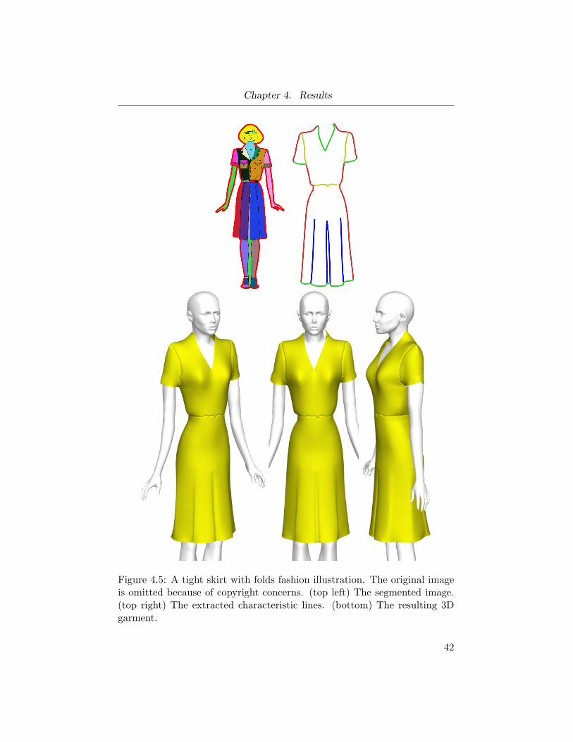
We decided to focus on women’s garments, as they tend to be muchmore interesting than men’s. We contracted an artist, Daichi Ito, fromAdobe Systems Incorporated to provide us with clean, front-facing garmentdrawings (Figures 4.1, 4.2, 4.3, 4.6 (head/hands)). Ito is a professionalartist, but not a professional fashion illustrator, and each drawing tookroughly half an hour. Using images from previously drawn, professionalfashion illustrations require that they can have lines successfully extractedfrom them. We chose two professional illustrations (Figures 4.4 and 4.5)that were able to be vectorized by Adobe Illustrator, so that the resultingbezier curves could be used for our drawing analysis algorithm. The originalscanned images for those two examples are omitted because of copyrightconcerns. Our remaining examples (Figures 4.7, 4.8, 4.9) were drawn directlyon a manequin using the interface of Turquin et al. [27].

It is difficult to devise an objective measure of evaluation for virtualgarments. While we believe the comparison with previous results speaks foritself, we are planning a user study to measure the plausibility of our resultsgiven the input images. One survey method would ask the participants todraw the profile silhouette of a garment given a front view, and comparetheir sketches to the profile silhouette of our results.

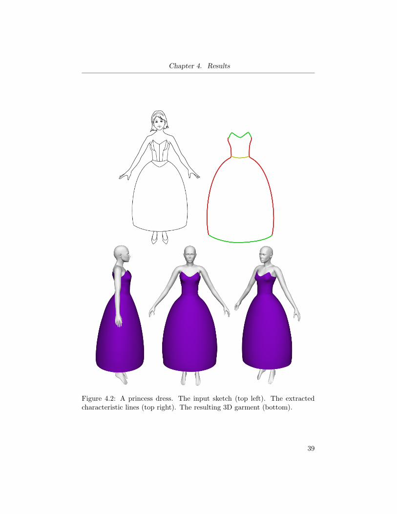
We have demonstrated the ability of our method to create a variety ofgarment shapes. The characteristic lines of the princess dress (Figure 4.2)

34

Chapter 4. Results

are relatively simple yet very clearly illustrate the different behavior of ourvirtual garments in tight and loose regions. The lower part of the dress puffsoutward, retaining a consistent silhouette from the front and side views. Thebodice, conversely, is very tight against the mannequin in the front view andso the garment follows the mannequin shape in the side view.

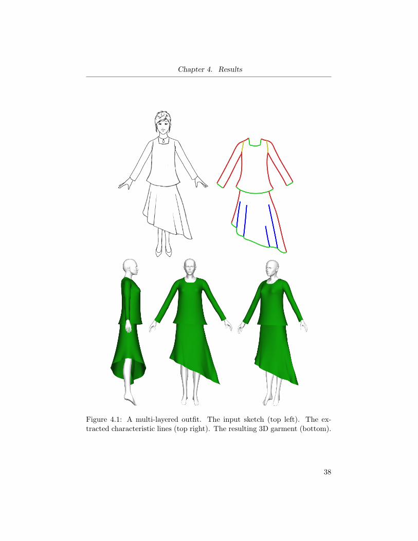
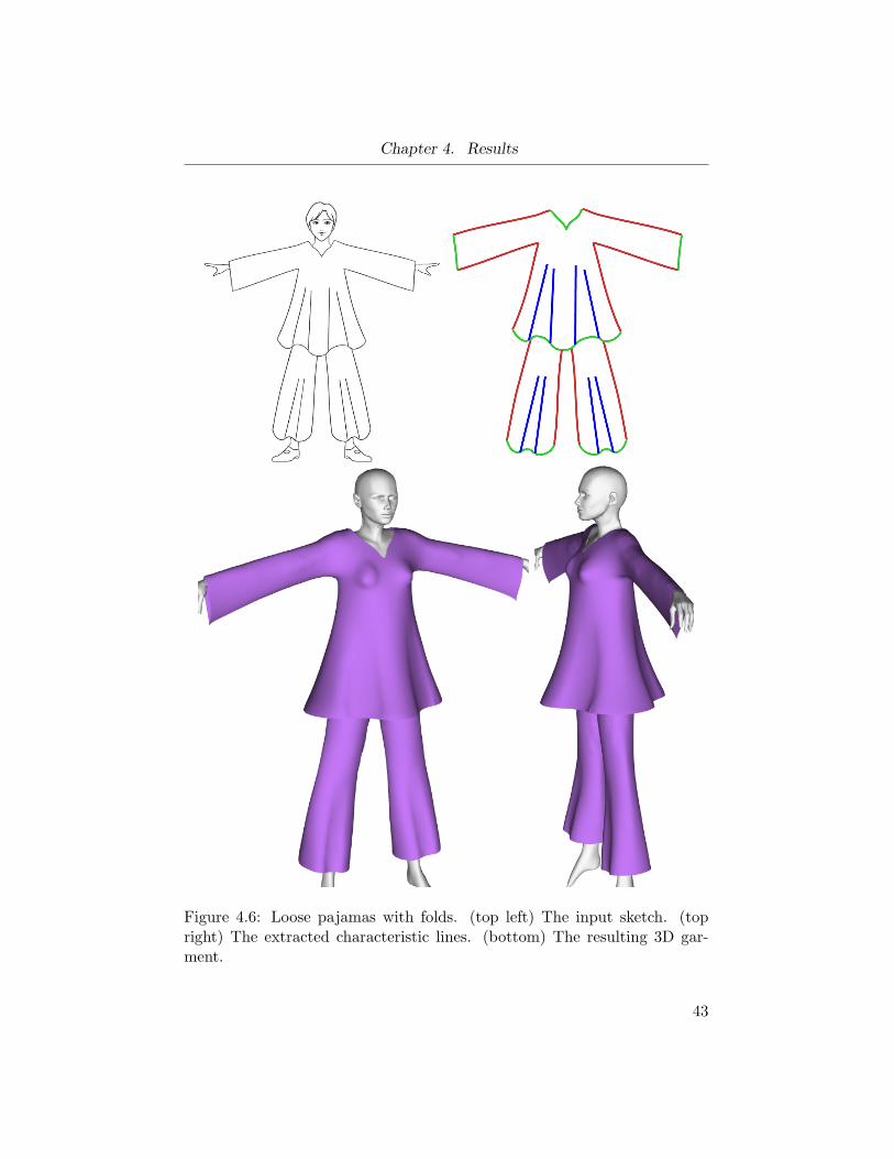
The multi-layered suit (Figure 4.1), shown at multiple stages earlier inthis document, demonstrates support for layered garments and asymmetrichems. Models of shirts and pants are shown in the example used to demon-strate the skeleton fitting stage (Figures 3.1 and 4.4) as well as the loosenightgown (Figure 4.6).

In most of these examples the drawing analysis was done fully automati-cally. There were two instances of user intervention needed for the drawingsshown in this document. First, in the ballgown drawing (Figure 4.2), wherethe perspective angle is very large, the boundary between silhouette (red)and border (green) lines on the bottom of the dress becomes very fuzzy.Thus, user intervention was necessary to identify the exact transition points.The second instance was in the pajama drawing (Figure 4.6). This garmentis very loose and the arms are raised fairly high leading the automatic skele-ton fitting algorithm to place the arms inside the shirt and converge to anincorrect local minimum. In this case, the user simply had to initialize theskeleton’s arms near those of the drawing and the skeleton fitting algorithmwas then able to converge to a successful fit. Other ambiguous inputs canbe resolved in similar manner.

The majority of the coefficients used in the optimizations performed byour system are fixed for all examples and we expect the specified defaultvalues to be applicable to all models. However, there are two parameterswhich we found users may want to control, developability γ and estimateddistance d from the viewer to the drawn figure (Section 3.3.2). The firstis strongly linked to the fabric and cut of the modeled garment, which canvary from model to model. For instance, for the princess dress (Figure 4.2)we turned the developability off, as we wanted the bodice to be very fitted.Figure 3.5 shows the impact of different values of γ. The distance value deffectively controls the depth of the garments at the hemlines. Our default

35

Chapter 4. Results

value works well for most models, but users may choose to modify it toobtain more or less puffy results, or turn it off altogether if the drawing hasno visible perspective.

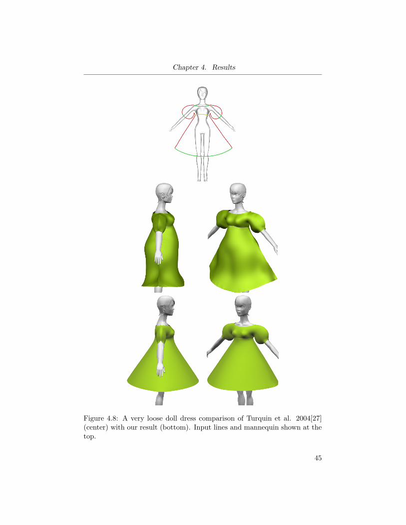
When comparing our results to those of previous methods [23, 27, 28]the differences are most prominent on loose garments. On these inputsthe garments created by our method appear noticeably more realistic andbetter reflect the input drawings. This is especially noticeable on the dolldress example in Figure 4.8. Notice how the garment from Turquin et al.[27] follows the mannequin’s body shape in front and behind, despite thefact that it is an extremely loose garment. Our method, on the other hand,maintains the same silhouette shape in the side view as found in the frontview. This is what we would expect from a loose garment, because the givenfront view silhouette shape is telling of the stiffness of the garment as wellas its expected behavior as it wraps around to the front and back. On tightgarments the difference is more subtle, however due to our use of mean andGaussian curvature minimizing terms in the wrapper modeling our garmentstend to be less “sticky” and thus more realistic in concave regions. Turquinet al.’s subsequent work in 2007 [28] added new features for folds and wavyhemlines (as referenced earlier in Figure 2.6), but the underlying garmentmodeling procedure, specifically the use of an offset surface, remains thesame and thus would create similar results to [27] given similar inputs.

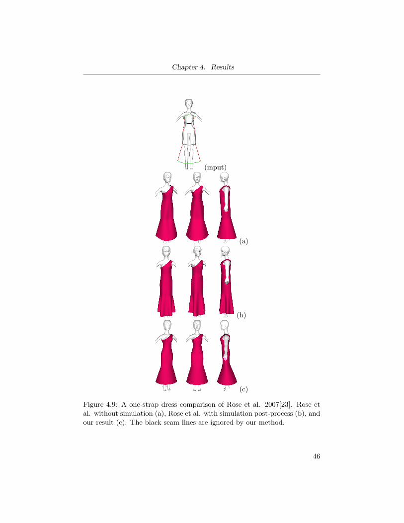
Figure 4.9 compares our results to those of Rose et al. [23]. The resultfrom Rose et al. is shown with and without a physical simulation postprocess. Their system uses the predefined seam lines and darts (lines ofnon-zero curvature) to divide the garment surface into developable pieceswhich are then modeled and stitched together. The developable property ofthe resulting surface allows their results to be manufactured as real-worldgarments. Despite this attractive property, the unsimulated result appearsunnaturally stiff in the side view. In contrast, the side view of our resultthe garment follows the mannequin shape in the tight region and retains thegarment’s front-view silhouette in the loose region. The result from Roseet al. with simulation has a natural cloth look, but now the garment nolonger matches the given characteristic lines in the front view, making the

36

Chapter 4. Results

modeling system less intuitive.Runtimes: The overall processing of the examples shown here takes on

the order of two to three minutes on a 2.13GHz Intel Core 2 CPU, with mostof the time spent in the skeleton fitting code. The modeling stage by itselftakes around 20 seconds processing meshes with about 50K triangles. Thususers who would want to use our system in an interactive setting where thefitting step is not necessary are looking at near-interactive reaction times.

37

Chapter 4. Results

Figure 4.1: A multi-layered outfit. The input sketch (top left). The ex-tracted characteristic lines (top right). The resulting 3D garment (bottom).

38

Chapter 4. Results

Figure 4.2: A princess dress. The input sketch (top left). The extractedcharacteristic lines (top right). The resulting 3D garment (bottom).

39

Chapter 4. Results

Figure 4.3: A basic schoolgirl skirt. The input sketch (top left). The ex-tracted characteristic lines (top right). The resulting 3D garment (bottom).

40

Chapter 4. Results

Figure 4.4: A tight shirt and pants outfit fashion illustration. The originalimage is omitted because of copyright concerns. (top left) The segmentedimage. (top right) The extracted characteristic lines. (bottom) The resulting3D garment.

41

Chapter 4. Results

Figure 4.5: A tight skirt with folds fashion illustration. The original imageis omitted because of copyright concerns. (top left) The segmented image.(top right) The extracted characteristic lines. (bottom) The resulting 3Dgarment.

42

Chapter 4. Results

Figure 4.6: Loose pajamas with folds. (top left) The input sketch. (topright) The extracted characteristic lines. (bottom) The resulting 3D gar-ment.

43

Chapter 4. Results

Figure 4.7: A tight Chinese dress comparison of Turquin et al. 2004[27](center) with our result (bottom). Input lines and mannequin shown at thetop.

44

Chapter 4. Results

Figure 4.8: A very loose doll dress comparison of Turquin et al. 2004[27](center) with our result (bottom). Input lines and mannequin shown at thetop.

45

Chapter 4. Results

(input)

(a)

(b)

(c)

Figure 4.9: A one-strap dress comparison of Rose et al. 2007[23]. Rose etal. without simulation (a), Rose et al. with simulation post-process (b), andour result (c). The black seam lines are ignored by our method.

46

Chapter 5

Discussion and Future Work

The primary contribution of this work is the introduction of a new garmentmodeling technique. It produces virtual garments that we believe to bebelievable interpretations of the sketched inputs. The garments are visuallyconsistent as they wrap around the mannequin in the front and back as wewould expect from real world garments. To demonstrate this novel modelingtechnique we have built a garment modeling system which is the first to usehand-drawn fashion illustrations as input. We accomplish this with a noveldrawing analysis algorithm that segments the drawing into key body andgarment regions, and estimates the figure’s pose with a mannequin fittingprocedure. This allows novice users to operate the garment modeling systemwithout needing to learn the specifics of tailoring or 3D modeling software.Additionally, this allows the virtual garment to be dressed on a mannequinwith an arbitrary pose inferred from the drawing, unlike previous onlinesketch-based modeling techniques that require a predefined mannequin.

We have leveraged a number of observations about how garments behaveand how people draw fashion illustrations to communicate garment shapein order to make this sketch-based modeling problem tractable. While theseobservations hold in most cases, exceptions can occur. For instance, somefashion illustrations may have the model posed at odd angles for stylisticreasons, or may have the model’s arms or legs occluded. To support thesetypes of inputs, the system could be extended to allow the user to adjust theskeleton in 3D during the drawing analysis phase. Later steps would onlyhave to make minor adjustments to accommodate a non-planar mannequinpose.

Another extension could allow the modeling of garments that are notsymmetric in the front and back. This could be done by either providing a

47

Chapter 5. Discussion and Future Work

back-view drawing to supplement the original front-view, or the user couldmanually edit the extracted characteristic lines for the back.

Beyond modeling just the garment shape, one could extend our system totexture the surface from the original drawing. The front should be more orless trivial, just being a texture map of the drawing itself, but the backsidewould provide a few challenges. One would have to detect what featurespresent on the front are most likely to propagate to the back. This is similarto research done in inpainting, where one must generate image details inone region given a surrounding image context. We speculate features likepockets would likely not propagate to the back, but seam lines or the shadingof folds at the bottom of a skirt would be a reasonable features to extend tothe back.

In future years, with more advance image analysis techniques, it shouldbe possible to extract sufficient information from a photograph of a fashionmodel or mannequin to generate a virtual garment. Perhaps given a videosequence of a model doing the iconic runway walk, enough views of the gar-ment could be tracked and captured to recreate a full virtual garment alongwith detailed animation properties. Furthermore, additional principals oftailoring and human body shape and pose could be leveraged to create evenmore sophisticated garment modeling techniques from fashion drawings orsketch-based software.

48

Bibliography

[1] Anne Allen and Julian Seaman. Fashion Drawing: The basic principles.Batsford, 2000.

[2] Alexandru O. Balan, Leonid Sigal, Michael J. Black, James E. Davis,and Horst W. Haussecker. Detailed human shape and pose from im-ages. Computer Vision and Pattern Recognition, IEEE Computer So-ciety Conference on, 0:1–8, 2007.

[3] David Bourguignon, Marie-Paule Cani, and George Drettakis. Draw-ing for illustration and annotation in 3d. Computer Graphics Forum,20(3):114–122, 2001.

[4] Philippe Decaudin, Dan Julius, Jamie Wither, Laurence Boissieux, AllaSheffer, and Marie-Paule Cani. Virtual garments: A fully geometric ap-proach for clothing design. Comput. Graph. Forum (Proc. Eurograph-ics’06), 25(3):625–634, 2006.

[5] Hongbo Fu, Yichen Wei, Chiew-Lan Tai, and Long Quan. Sketchinghairstyles. In SBIM ’07: Proceedings of the 4th Eurographics workshopon Sketch-based interfaces and modeling, pages 31–36, New York, NY,USA, 2007. ACM.

[6] Google. Google Sketchup http://sketchup.google.com/.

[7] Haute Couture 3D. http://www.gcldistribution.com/en/haute couture 3d.html.

[8] Donald H. House and David E. Breen, editors. Cloth modeling andanimation. A. K. Peters, Ltd., Natick, MA, USA, 2000.

49

Chapter 5. Bibliography

[9] Takeo Igarashi and John F. Hughes. Clothing manipulation. In Proc.UIST”02, pages 91–100, 2002.

[10] Takeo Igarashi, Satoshi Matsuoka, and Hidehiko Tanaka. Teddy: Asketching interface for 3d freeform design. pages 409–416, 1999.

[11] P. J. Ireland. Fashion Desing Drawing and Presentation. Batsford,1989.

[12] O. A. Karpenko and J. Hughes. Smoothsketch:3D free-form shapesfrom complex sketches. ACM Transactions on Graphics, 25(3):589–598, 2006.

[13] Yaron Lipman, Olga Sorkine, David Levin, and Daniel Cohen-Or. Lin-ear rotation-invariant coordinates for meshes. In Proc. SIGGRAPH ’05,pages 479–487, 2005.

[14] S. Mauch and D. Breen. A fast algorithm for computing the closestpoint and distance function. Technical report, 2000.

[15] MayaCloth. http://caad.arch.ethz.ch /info/maya/manual/MayaCloth (accessed

2009).

[16] Yuki Mori and Takeo Igarashi. Plushie: an interactive design systemfor plush toys. In Proc. SIGGRAPH’07, pages 45–54, New York, NY,USA, 2007.

[17] Pascal Muller, Peter Wonka, Simon Haegler, Andreas Ulmer, and LucVan Gool. Procedural modeling of buildings. ACM Trans. Graph.,25(3):614–623, 2006.

[18] Andrew Nealen, Takeo Igarashi, Olga Sorkine, and Marc Alexa. Fiber-mesh: designing freeform surfaces with 3d curves. ACM Trans. Graph.,26(3):41, 2007.

[19] Diego Nehab, Szymon Rusinkiewicz, James Davis, and Ravi Ra-mamoorthi. Efficiently combining positions and normals for precise 3D

50


geometry. ACM Transactions on Graphics (Proc. of ACM SIGGRAPH2005), 24(3), 2005.

[20] Luke Olsen, Faramarz F. Samavati, Mario Costa Sousa, and Joaquim A.Jorge. Sketch-based modeling: A survey. Computers and Graphics,33(1):85 – 103, 2009.

[21] Sylvain Paris, Will Chang, Oleg I. Kozhushnyan, Wojciech Jarosz, Woj-ciech Matusik, Matthias Zwicker, and Fredo Durand. Hair photobooth:geometric and photometric acquisition of real hairstyles. In Proc. SIG-GRAPH ’08, pages 1–9. ACM, 2008.

[22] Long Quan, Ping Tan, Gang Zeng, Lu Yuan, Jingdong Wang, andSing Bing Kang. Image-based plant modeling. ACM Trans. Graph.,25(3):599–604, 2006.

[23] Kenneth Rose, Alla Sheffer, Jamie Wither, Marie-Paule Cani, and BorisThibert. Developable surfaces from arbitrary sketched boundaries. InProc. Eurographics Symposium on Geometry Processing, 2007.

[24] Sudipta N. Sinha, Drew Steedly, Richard Szeliski, Maneesh Agrawala,and Marc Pollefeys. Interactive 3d architectural modeling from un-ordered photo collections. ACM Trans. Graph., 27(5):1–10, 2008.

[25] Ivan E. Sutherland. Sketch pad a man-machine graphical communica-tion system. In DAC ’64: Proceedings of the SHARE design automationworkshop, pages 6.329–6.346, New York, NY, USA, 1964. ACM.

[26] Sivan Toledo, Doron Chen, and Vladimir Rotkin. Taucs: A library ofsparse linear solvers, 2003. http://www.tau.ac.il/ stoledo/taucs/.

[27] Emmanuel Turquin, Marie-Paule Cani, and John F. Hughes. Sketchinggarments for virtual characters . In Proc. Eurographics Workshop onSketch-Based Interfaces and Modeling, pages 175–182, 2004.

[28] Emmanuel Turquin, Jamie Wither, Laurence Boissieux, Marie-PauleCani, and John F. Hughes. A sketch-based interface for clothing virtualcharacters. IEEE Comput. Graph. Appl., 27(1):72–81, 2007.

51


[29] Daniel Vlasic, Ilya Baran, Wojciech Matusik, and Jovan Popovic. Ar-ticulated mesh animation from multi-view silhouettes. ACM Trans.Graph., 27(3):97–106, 2008.

[30] Charlie Wang, Yu Wang, and Matthew Yuen. Feature based 3d garmentdesign through 2d sketches. Computer-Aided Design, 35:659–672, 2003.

[31] Chen Yang, Dana Sharon, and Michiel van de Panne. Sketch-basedmodeling of parameterized objects. In SBIM ’05: Proceedings of the2nd Eurographics Workshop on Sketch-based Interfaces and Modeling,Dublin, 2005.

52

garment modeling from fashion drawings and sketches · our free-hand drawing analysis setup and in...

Documents