gamma dbms (part 2): failure management query processing shahram ghandeharizadeh computer science...
TRANSCRIPT

Gamma DBMS (Part 2): Gamma DBMS (Part 2): Failure ManagementFailure ManagementQuery ProcessingQuery Processing
Shahram GhandeharizadehShahram GhandeharizadehComputer Science DepartmentComputer Science DepartmentUniversity of Southern CaliforniaUniversity of Southern California
Failure Management TechniquesFailure Management Techniques
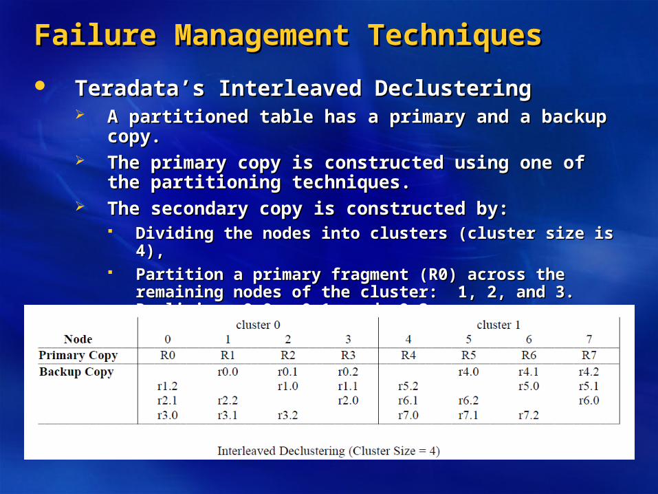
Teradata’s Interleaved DeclusteringTeradata’s Interleaved Declustering A partitioned table has a primary and a backup copy.A partitioned table has a primary and a backup copy. The primary copy is constructed using one of the The primary copy is constructed using one of the
partitioning techniques.partitioning techniques. The secondary copy is constructed by:The secondary copy is constructed by:
Dividing the nodes into clusters (cluster size is 4),Dividing the nodes into clusters (cluster size is 4), Partition a primary fragment (R0) across the remaining nodes Partition a primary fragment (R0) across the remaining nodes
of the cluster: 1, 2, and 3. Realizing r0.0, r0.1, and r0.2.of the cluster: 1, 2, and 3. Realizing r0.0, r0.1, and r0.2.
Teradata’s Interleaved DeclusteringTeradata’s Interleaved Declustering
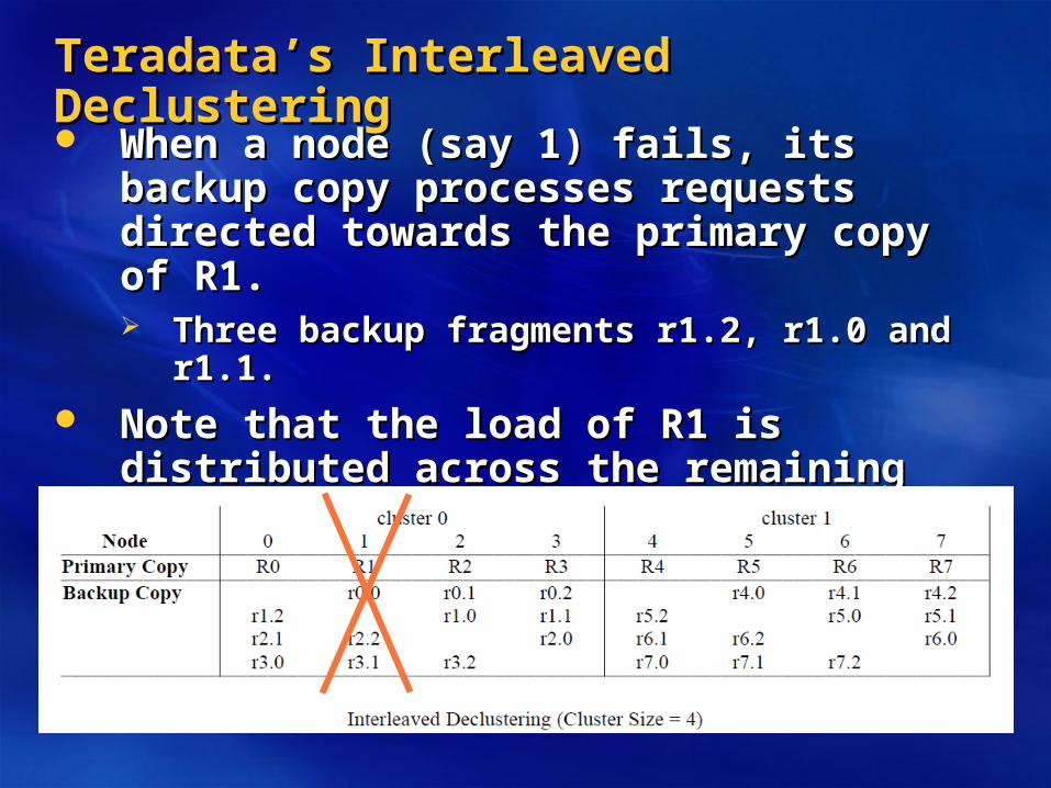
When a node (say 1) fails, its backup copy When a node (say 1) fails, its backup copy processes requests directed towards the processes requests directed towards the primary copy of R1.primary copy of R1. Three backup fragments r1.2, r1.0 and r1.1.Three backup fragments r1.2, r1.0 and r1.1.
Note that the load of R1 is distributed across Note that the load of R1 is distributed across the remaining nodes of the cluster.the remaining nodes of the cluster.

Teradata’s Interleaved DeclusteringTeradata’s Interleaved Declustering
MTTR involves:MTTR involves:1.1. Replacing the failed node with a new one.Replacing the failed node with a new one.
2.2. Reconstructing the primary copy of the fragment Reconstructing the primary copy of the fragment assigned to the failed node, R1.assigned to the failed node, R1. By reading r1.2, r1.0, and r1.1 from Nodes 0, 2, and 3.By reading r1.2, r1.0, and r1.1 from Nodes 0, 2, and 3.
3.3. Reconstructing the backup fragments assigned Reconstructing the backup fragments assigned to the failed node: r0.0, r2.2, and r3.1.to the failed node: r0.0, r2.2, and r3.1.
Teradata’s Interleaved DeclusteringTeradata’s Interleaved Declustering
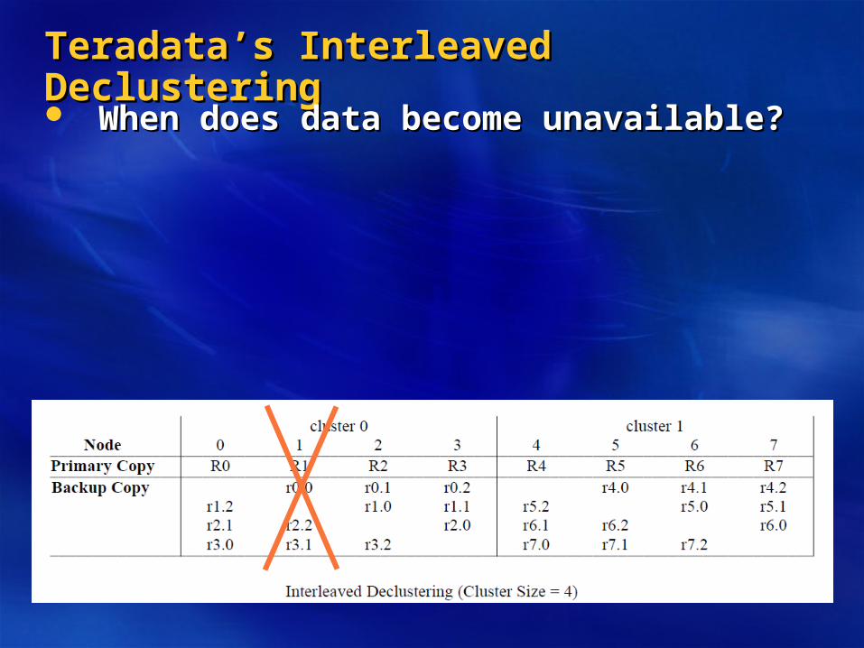
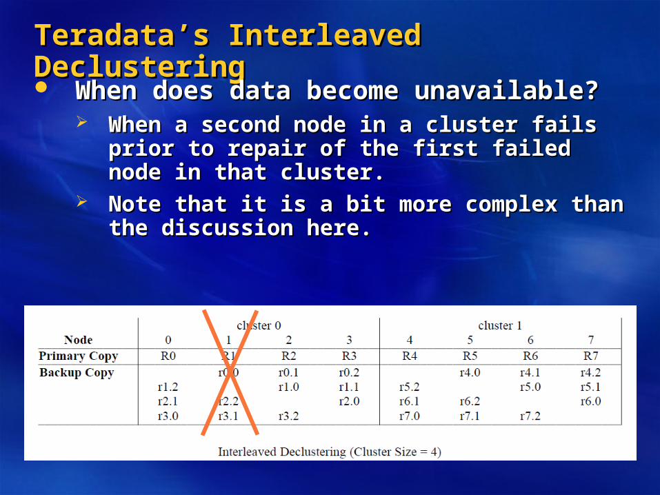
When does data become unavailable?When does data become unavailable?
Teradata’s Interleaved DeclusteringTeradata’s Interleaved Declustering
When does data become unavailable?When does data become unavailable? When a second node in a cluster fails prior to When a second node in a cluster fails prior to
repair of the first failed node in that cluster.repair of the first failed node in that cluster. Note that it is a bit more complex than the Note that it is a bit more complex than the
discussion here.discussion here.

Teradata’s Interleaved DeclusteringTeradata’s Interleaved Declustering
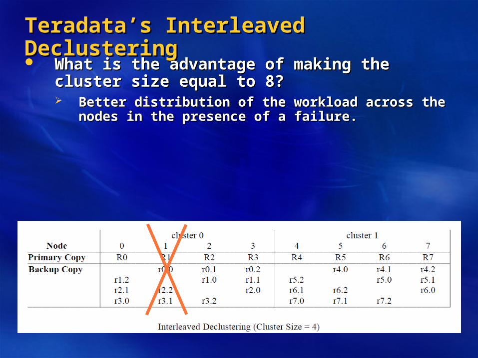
What is the advantage of making the cluster size What is the advantage of making the cluster size equal to 8?equal to 8?
Teradata’s Interleaved DeclusteringTeradata’s Interleaved Declustering
What is the advantage of making the cluster size What is the advantage of making the cluster size equal to 8?equal to 8? Better distribution of the workload across the nodes in the Better distribution of the workload across the nodes in the
presence of a failure.presence of a failure.
Teradata’s Interleaved DeclusteringTeradata’s Interleaved Declustering
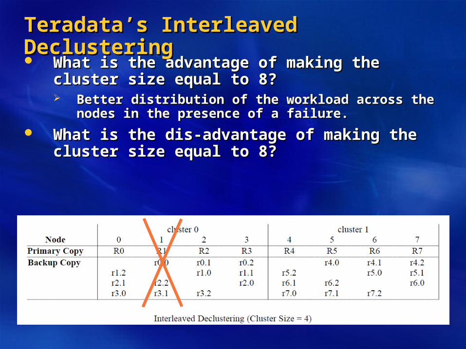
What is the advantage of making the cluster size What is the advantage of making the cluster size equal to 8?equal to 8? Better distribution of the workload across the nodes in the Better distribution of the workload across the nodes in the
presence of a failure.presence of a failure.
What is the dis-advantage of making the cluster size What is the dis-advantage of making the cluster size equal to 8?equal to 8?
Teradata’s Interleaved DeclusteringTeradata’s Interleaved Declustering
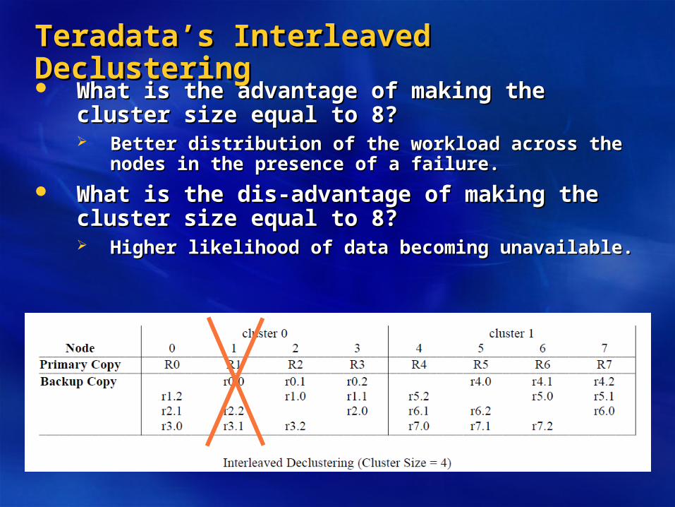
What is the advantage of making the cluster size What is the advantage of making the cluster size equal to 8?equal to 8? Better distribution of the workload across the nodes in the Better distribution of the workload across the nodes in the
presence of a failure.presence of a failure.
What is the dis-advantage of making the cluster size What is the dis-advantage of making the cluster size equal to 8?equal to 8? Higher likelihood of data becoming unavailable.Higher likelihood of data becoming unavailable.

Teradata’s Interleaved DeclusteringTeradata’s Interleaved Declustering
What is the advantage of making the cluster size What is the advantage of making the cluster size equal to 8?equal to 8? Better distribution of the workload across the nodes in the Better distribution of the workload across the nodes in the
presence of a failure.presence of a failure.
What is the dis-advantage of making the cluster size What is the dis-advantage of making the cluster size equal to 8?equal to 8? Higher likelihood of data becoming unavailable.Higher likelihood of data becoming unavailable.
Tradeoff between load-balancing (in the presence of Tradeoff between load-balancing (in the presence of a failure) and data availability.a failure) and data availability.
Gamma’s Chained DeclusteringGamma’s Chained Declustering
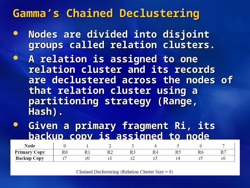
Nodes are divided into disjoint groups called Nodes are divided into disjoint groups called relation clusters.relation clusters.
A relation is assigned to one relation cluster A relation is assigned to one relation cluster and its records are declustered across the and its records are declustered across the nodes of that relation cluster using a nodes of that relation cluster using a partitioning strategy (Range, Hash).partitioning strategy (Range, Hash).
Given a primary fragment Ri, its backup Given a primary fragment Ri, its backup copy is assigned to node copy is assigned to node (i+1) mod M(i+1) mod M (M is (M is the number of nodes in the relation cluster).the number of nodes in the relation cluster).
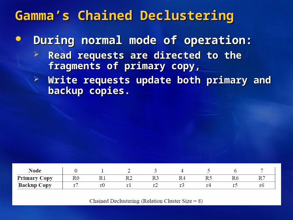
Gamma’s Chained DeclusteringGamma’s Chained Declustering
During normal mode of operation:During normal mode of operation: Read requests are directed to the fragments of Read requests are directed to the fragments of
primary copy,primary copy, Write requests update both primary and backup Write requests update both primary and backup
copies.copies.

Gamma’s Chained DeclusteringGamma’s Chained Declustering In the presence of failure:In the presence of failure:
Both primary and backup fragments are used for read Both primary and backup fragments are used for read operations,operations, Objective: Balance the load and avoid bottlenecks!Objective: Balance the load and avoid bottlenecks!
Write requests update both primary and backup copies.Write requests update both primary and backup copies.
Note:Note: Load of R1 (on node 1) is pushed to node 2 in its entirety.Load of R1 (on node 1) is pushed to node 2 in its entirety. A fraction of read request from each node is pushed to the A fraction of read request from each node is pushed to the
others for a 1/8 load increase attributed to node 1’s failure.others for a 1/8 load increase attributed to node 1’s failure.

Gamma’s Chained DeclusteringGamma’s Chained Declustering MTTR involves:MTTR involves:
Replace node 1 with a new node,Replace node 1 with a new node, Reconstruct R1 (from r1 on node 2) on node 1,Reconstruct R1 (from r1 on node 2) on node 1, Reconstruct backup copy of R0 (i.e., r0) on node 1.Reconstruct backup copy of R0 (i.e., r0) on node 1.
Note:Note: Once Node 1 becomes operational, primary copies are Once Node 1 becomes operational, primary copies are
used to process read requests.used to process read requests.
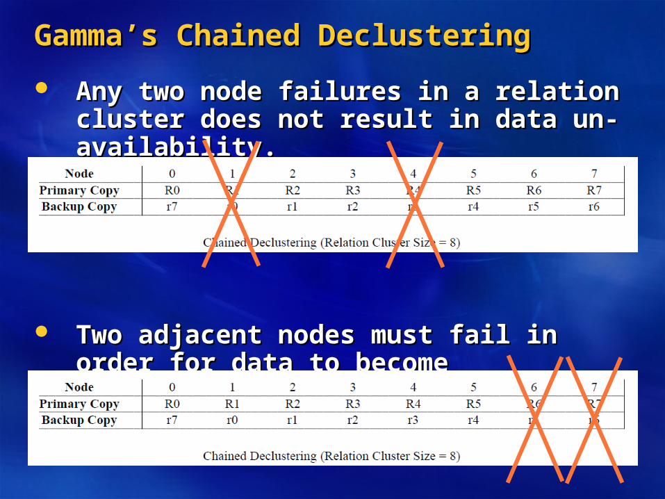
Gamma’s Chained DeclusteringGamma’s Chained Declustering
Any two node failures in a relation cluster Any two node failures in a relation cluster does not result in data un-availability.does not result in data un-availability.
Two adjacent nodes must fail in order for Two adjacent nodes must fail in order for data to become unavailable.data to become unavailable.
Gamma’s Chained DeclusteringGamma’s Chained Declustering
Re-assignment of active fragments incurs Re-assignment of active fragments incurs neither disk I/O nor data movement.neither disk I/O nor data movement.

JoinJoin
Hash-join Hash-join A data-flow execution paradigmA data-flow execution paradigm

Example Join of Emp and DeptExample Join of Emp and Dept
Emp join Dept (using dno)Emp join Dept (using dno)
SS#SS# NameName AgeAge SalarySalary dnodno
11 JoeJoe 2424 2000020000 22
22 MaryMary 2020 2500025000 11
33 BobBob 2222 2700027000 11
44 KathyKathy 3030 3000030000 22
55 ShidehShideh 44 40004000 11
EMP
dnodno dnamedname floorfloor mgrss#mgrss#
11 ToyToy 11 55
22 ShoeShoe 22 11
Dept
SS#SS# NameName AgeAge SalarySalary dnodno dnamedname floorfloor mgrss#mgrss#
11 JoeJoe 2424 2000020000 22 ShoeShoe 22 11
22 MaryMary 2020 2500025000 11 ToyToy 11 55
33 BobBob 2222 2700027000 11 ToyToy 11 55
44 KathyKathy 3030 3000030000 22 ShoeShoe 22 11
55 ShidehShideh 44 40004000 11 ToyToy 11 55

Hash-Join: 1 NodeHash-Join: 1 Node
Join of Tables A and B using attribute j (A.j = Join of Tables A and B using attribute j (A.j = B.j) consists of two phase:B.j) consists of two phase:1.1. Build phase: Build a main-memory hash table on Build phase: Build a main-memory hash table on
Table A using the join attribute j, e.g., build a Table A using the join attribute j, e.g., build a hash table on the Toy department using dno as hash table on the Toy department using dno as the key of the hash table.the key of the hash table.
2.2. Probe phase: Scan table B one record at a time Probe phase: Scan table B one record at a time and use its attribute j to probe the hash table and use its attribute j to probe the hash table constructed on Table A, e.g., probe the hash constructed on Table A, e.g., probe the hash table using the rows of the Emp department.table using the rows of the Emp department.
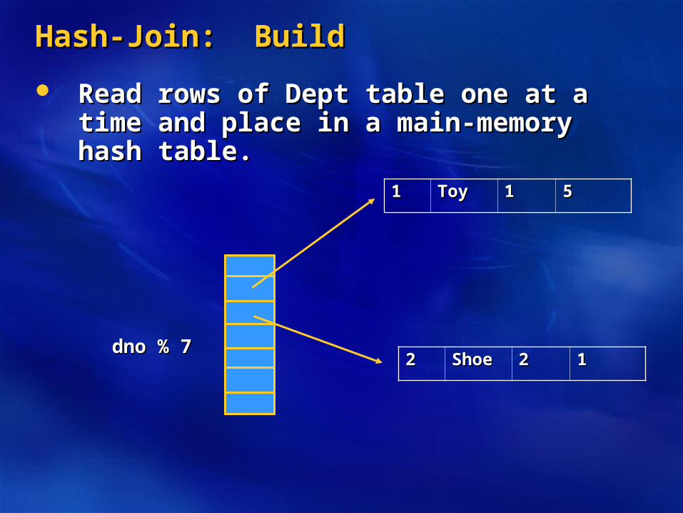
Hash-Join: BuildHash-Join: Build
Read rows of Dept table one at a time and Read rows of Dept table one at a time and place in a main-memory hash table.place in a main-memory hash table.
11 ToyToy 11 55
22 ShoeShoe 22 11dno % 7dno % 7

Hash-Join: BuildHash-Join: Build
Read rows of Emp table and probe the hash table.Read rows of Emp table and probe the hash table.
11 ToyToy 11 55
22 ShoeShoe 22 11dno % 7dno % 7
SS#SS# NameName AgeAge SalarySalary dnodno
11 JoeJoe 2424 2000020000 22

Hash-Join: BuildHash-Join: Build
Read rows of Emp table and probe the hash table Read rows of Emp table and probe the hash table and produce results when a match is found.and produce results when a match is found.
SS#SS# NameName AgeAge SalarySalary dnodno
11 JoeJoe 2424 2000020000 22 11 ToyToy 11 55
22 ShoeShoe 22 11dno % 7dno % 7
SS#SS# NameName AgeAge SalarySalary dnodno dnamedname floorfloor mgrss#mgrss#
11 JoeJoe 2424 2000020000 22 ShoeShoe 22 11
Hash-Join: BuildHash-Join: Build
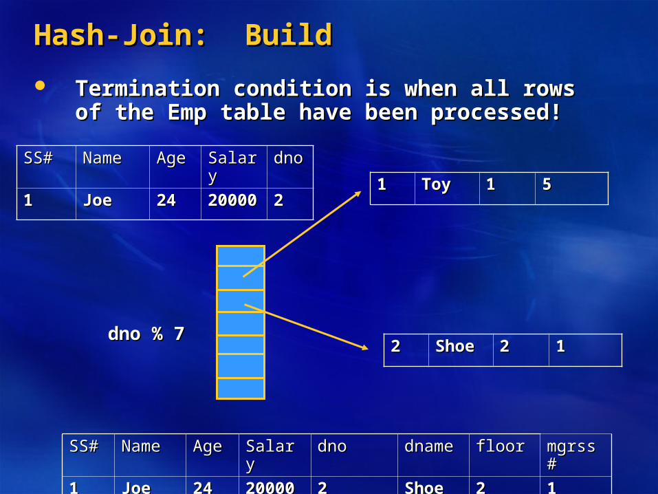
Termination condition is when all rows of the Emp Termination condition is when all rows of the Emp table have been processed!table have been processed!
SS#SS# NameName AgeAge SalarySalary dnodno
11 JoeJoe 2424 2000020000 22 11 ToyToy 11 55
22 ShoeShoe 22 11dno % 7dno % 7
SS#SS# NameName AgeAge SalarySalary dnodno dnamedname floorfloor mgrss#mgrss#
11 JoeJoe 2424 2000020000 22 ShoeShoe 22 11

Hash-JoinHash-Join
Key challenge:Key challenge:
Hash-JoinHash-Join
Key challenge: Table used to build the hash table Key challenge: Table used to build the hash table does not fit in main memory!does not fit in main memory!
Solution:Solution:
Hash-JoinHash-Join
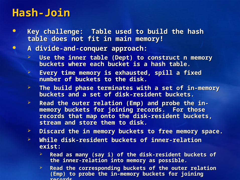
Key challenge: Table used to build the hash table does not fit Key challenge: Table used to build the hash table does not fit in main memory!in main memory!
A divide-and-conquer approach:A divide-and-conquer approach: Use the inner table (Dept) to construct n memory buckets where Use the inner table (Dept) to construct n memory buckets where
each bucket is a hash table.each bucket is a hash table. Every time memory is exhausted, spill a fixed number of Every time memory is exhausted, spill a fixed number of
buckets to the disk.buckets to the disk. The build phase terminates with a set of in-memory buckets and The build phase terminates with a set of in-memory buckets and
a set of disk-resident buckets.a set of disk-resident buckets. Read the outer relation (Emp) and probe the in-memory buckets Read the outer relation (Emp) and probe the in-memory buckets
for joining records. For those records that map onto the disk-for joining records. For those records that map onto the disk-resident buckets, stream and store them to disk.resident buckets, stream and store them to disk.
Discard the in memory buckets to free memory space.Discard the in memory buckets to free memory space. While disk-resident buckets of inner-relation exist:While disk-resident buckets of inner-relation exist:
Read as many (say i) of the disk-resident buckets of the inner-Read as many (say i) of the disk-resident buckets of the inner-relation into memory as possible.relation into memory as possible.
Read the corresponding buckets of the outer relation (Emp) to probe Read the corresponding buckets of the outer relation (Emp) to probe the in-memory buckets for joining records.the in-memory buckets for joining records.
Discard the in memory buckets to free memory space.Discard the in memory buckets to free memory space. Delete the i buckets of the inner and outer relations.Delete the i buckets of the inner and outer relations.
Hash-Join: BuildHash-Join: Build
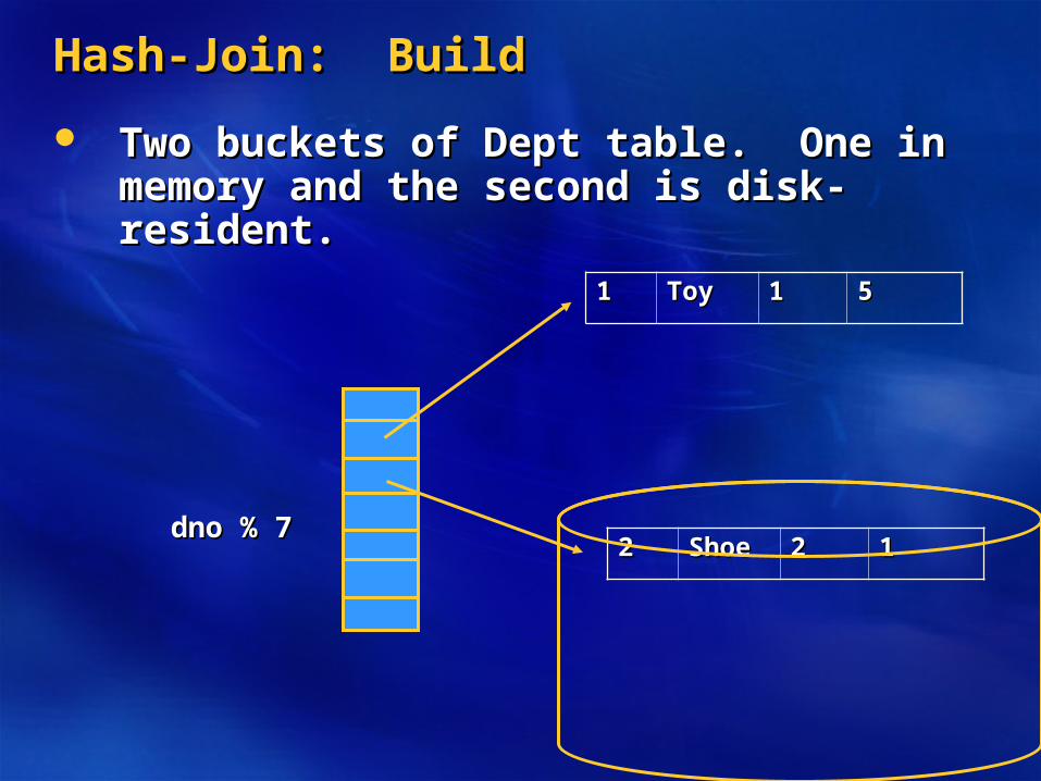
Two buckets of Dept table. One in memory Two buckets of Dept table. One in memory and the second is disk-resident.and the second is disk-resident.
11 ToyToy 11 55
22 ShoeShoe 22 11dno % 7dno % 7
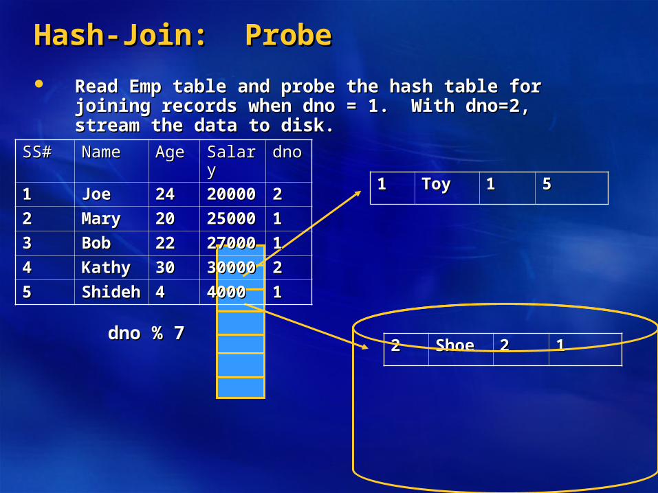
Hash-Join: ProbeHash-Join: Probe
Read Emp table and probe the hash table for joining records Read Emp table and probe the hash table for joining records when dno = 1. With dno=2, stream the data to disk.when dno = 1. With dno=2, stream the data to disk.
11 ToyToy 11 55
22 ShoeShoe 22 11dno % 7dno % 7
SS#SS# NameName AgeAge SalarySalary dnodno
11 JoeJoe 2424 2000020000 22
22 MaryMary 2020 2500025000 11
33 BobBob 2222 2700027000 11
44 KathyKathy 3030 3000030000 22
55 ShidehShideh 44 40004000 11
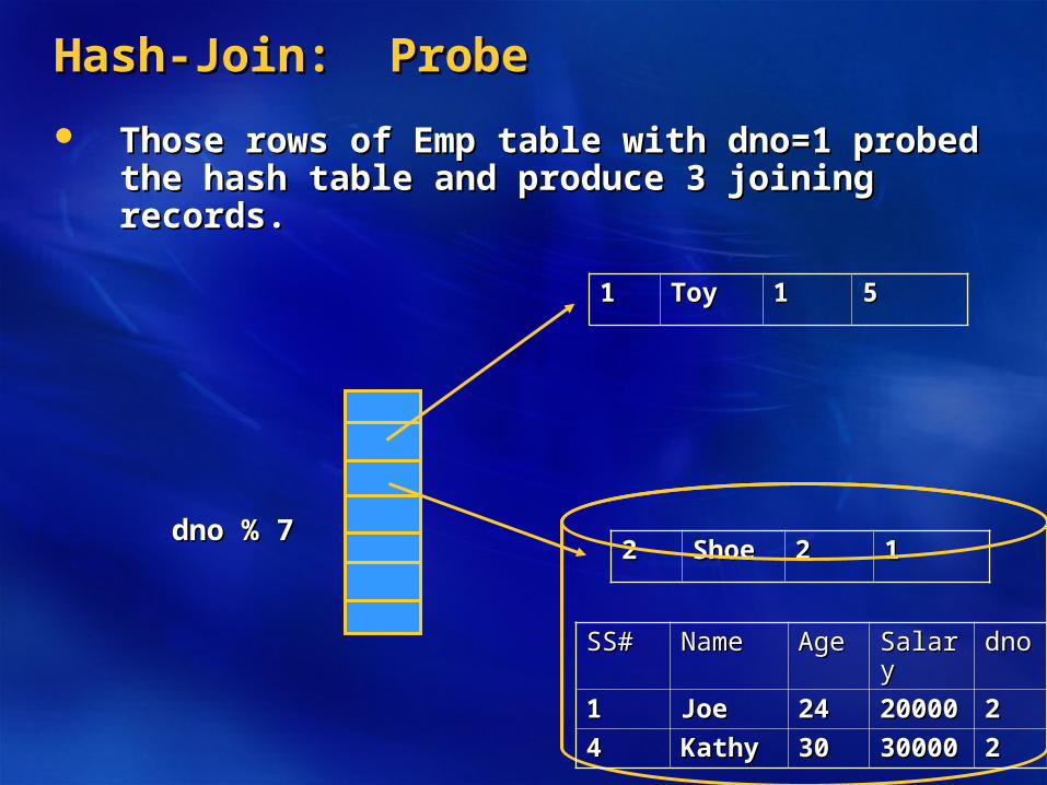
Hash-Join: ProbeHash-Join: Probe
Those rows of Emp table with dno=1 probed the Those rows of Emp table with dno=1 probed the hash table and produce 3 joining records.hash table and produce 3 joining records.
11 ToyToy 11 55
22 ShoeShoe 22 11dno % 7dno % 7
SS#SS# NameName AgeAge SalarySalary dnodno
11 JoeJoe 2424 2000020000 22
44 KathyKathy 3030 3000030000 22
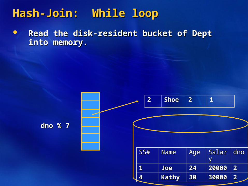
Hash-Join: While loopHash-Join: While loop
Read the disk-resident bucket of Dept into memory.Read the disk-resident bucket of Dept into memory.
22 ShoeShoe 22 11
dno % 7dno % 7
SS#SS# NameName AgeAge SalarySalary dnodno
11 JoeJoe 2424 2000020000 22
44 KathyKathy 3030 3000030000 22
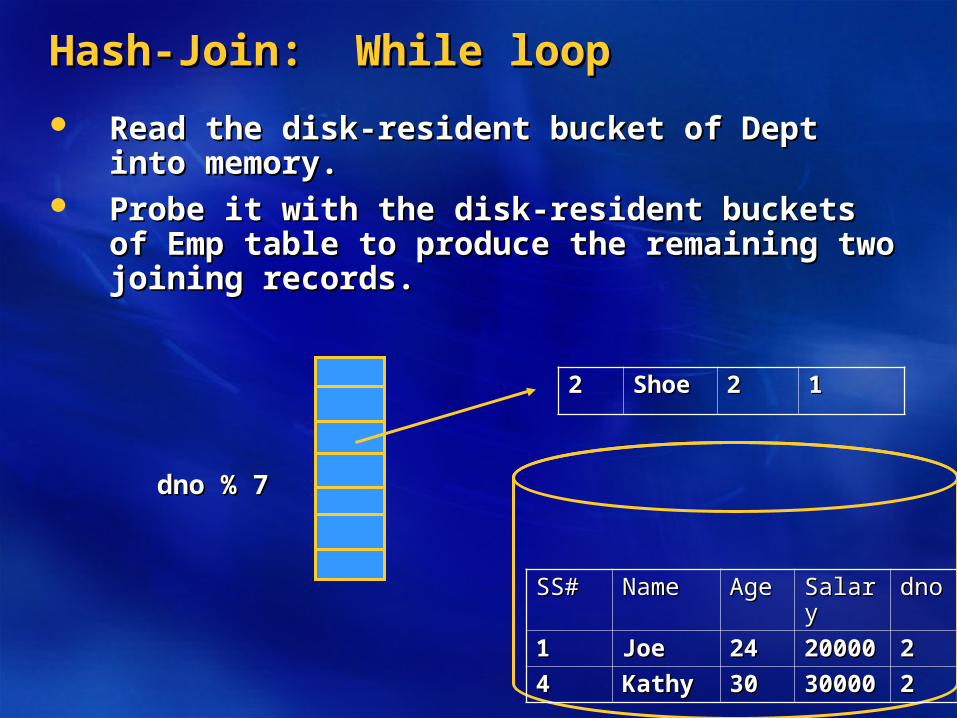
Hash-Join: While loopHash-Join: While loop
Read the disk-resident bucket of Dept into memory.Read the disk-resident bucket of Dept into memory. Probe it with the disk-resident buckets of Emp table Probe it with the disk-resident buckets of Emp table
to produce the remaining two joining records.to produce the remaining two joining records.
22 ShoeShoe 22 11
dno % 7dno % 7
SS#SS# NameName AgeAge SalarySalary dnodno
11 JoeJoe 2424 2000020000 22
44 KathyKathy 3030 3000030000 22

Parallelism and Hash-JoinParallelism and Hash-Join
Each node may perform hash-join Each node may perform hash-join independently when:independently when: The join attribute is the declustering attribute of The join attribute is the declustering attribute of
the tables participating in the join operation.the tables participating in the join operation. The participating tables are declustered across The participating tables are declustered across
the same number of nodes using the same the same number of nodes using the same declustering strategy.declustering strategy.
The system may re-partition the table (see the The system may re-partition the table (see the next bullet) if its aggregate memory exceeds the next bullet) if its aggregate memory exceeds the size of memory the tables are declustered size of memory the tables are declustered across.across.
Otherwise, the data must be re-partitioned to Otherwise, the data must be re-partitioned to perform the join operation correctly.perform the join operation correctly.
Show an example!Show an example!
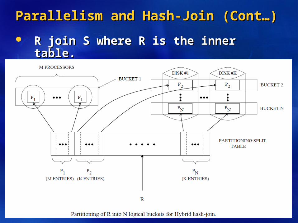
Parallelism and Hash-Join (Cont…)Parallelism and Hash-Join (Cont…)
R join S where R is the inner table.R join S where R is the inner table.
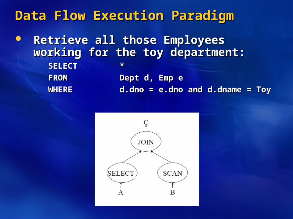
Data Flow Execution ParadigmData Flow Execution Paradigm
Retrieve all those Employees working for the Retrieve all those Employees working for the toy department:toy department:
SELECT SELECT **
FROM FROM Dept d, Emp eDept d, Emp e
WHERE WHERE d.dno = e.dno and d.dname = Toyd.dno = e.dno and d.dname = Toy
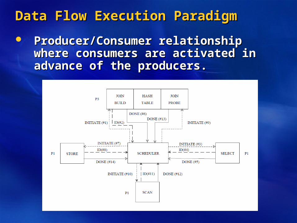
Data Flow Execution ParadigmData Flow Execution Paradigm
Producer/Consumer relationship where Producer/Consumer relationship where consumers are activated in advance of the consumers are activated in advance of the producers.producers.
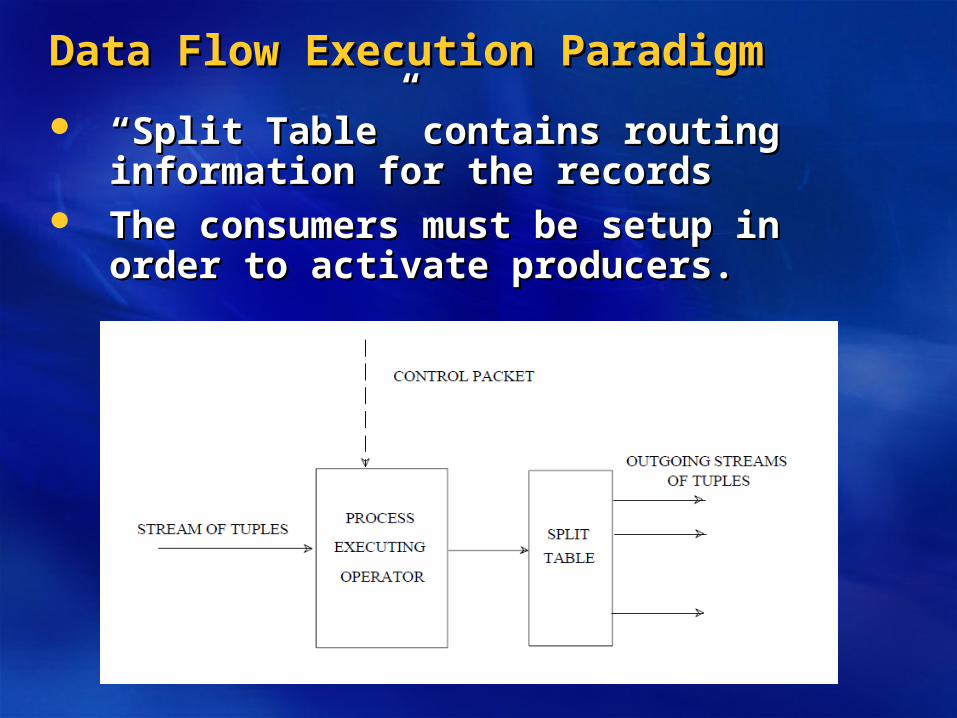
Data Flow Execution ParadigmData Flow Execution Paradigm
““Split Table” contains routing information Split Table” contains routing information for the recordsfor the records
The consumers must be setup in order to The consumers must be setup in order to activate producers.activate producers.