galerkin finite element method and finite difference method for solving...

Ciência/Science

Engenharia Térmica (Thermal Engineering), Vol. 9 • No 01 e 02 • December 2010 • p. 69-73 69

GALERKIN FINITE ELEMENT METHOD AND FINITE

DIFFERENCE METHOD FOR SOLVING

CONVECTIVE NON-LINEAR EQUATION

E. C. Romãoa,

M. D. de Camposb,

and L. F. M. de Mourab

aUniversidade Federal de Itajubá

Campus Avançado de Itabira

Rua Irmão Ivone Drumond, 200

Distrito Industrial II

CEP 35903-087 Itabira MG Brasil

[email protected]

bUniversidade Estadual de Campinas

Faculdade de Engenharia Mecânica

Departamento de Engenharia Térmica e

Fluidos

Rua Mendeleyev, 200

Cidade Universitária "Zeferino Vaz"

Distrito de Barão Geraldo

CEP:13083-860 Campinas SP Brasil

ABSTRACT The fast progress has been observed in the development of numerical and

analytical techniques for solving convection-diffusion and fluid mechanics

problems. Here, a numerical approach, based in Galerkin Finite Element

Method with Finite Difference Method is presented for the solution of a

class of non-linear transient convection-diffusion problems. Using the

analytical solutions and the L2 and L∞ error norms, some applications is

carried and valuated with the literature.

Keywords: Numerical simulation, Burgers’ equation, Galerkin Finite

Element Method, Finite Difference Method, Cranck-Nicolson Method.

NOMENCLATURE

x e y space coordinates

t time coordinate

Nj interpolation function

Nnodes number of nodes in each finite element

u velocity eju velocity approximation in the finite element

Greek symbols

Ω one-dimensional domain eΩ one-dimensional domain in the element

α coefficient of Crank-Nicholson Method

ξ local coordinate

Subscripts

node identification of a node

1. INTRODUCTION

The majority of problems in fluid mechanics and

heat transfer are represented by nonlinear partial

differential equations. A classical nonlinear first-

order hyperbolic equation inicially proposed by

Bateman in 1915, later on was treated by Burgers in

1948, after whom this equation is widely referred to

as Burgers’ equation, a important role in the study of

nonlinear waves since it can be used as mathematical

model of free turbulence (Kevorkian, 1990). Besides,

is also a model example for important applications in

physical phenomena such as acoustics, continuous

stochastic processes, dispersive water waves, gas

dynamics, heat conduction, longitudinalelastic waves

in an isotropic solid, number theory, shock waves,

turbulence and so forth (Polyanin and Zaitsev, 2004).

In recent years, many researchers have proposed

various kinds of numerical methods for Burgers’

equation (Dogan, 2004; Dag et al., 2005; Zhang et

Ciência/Science Romão et al. Galerkin Finite Element Method …

70 Engenharia Térmica (Thermal Engineering), Vol. 9 • No 01 e 02 • December 2010 • p. 69-73

al., 2009; Xu et al., 2011), mainly concerned with the

development of computational algorithms where, in a

continuous drive to demonstrate the superior

accuracy and stability properties of their latest

numerical method, for numerical solution.

It is one of a few well-known nonlinear partial

differential equations, which can be solved

analytically on the restricted initial conditions (Guo-

Zhong et al., 2010).

The Burgers’ equation is give by

2

2

Re

1

x

u

x

uu

t

u

∂

∂=

∂∂

+∂∂

(1)

In 1950 and 1951, E. Hopf and J. D. Cole

independently showed that Eq. (1) can be

transformed in the linear diffusion equation

(Kevorkian, 1990). Thus, we can rewrite the Eq.(1) as

follows

2Re

1

x

u

x

E

t

u

∂

∂+

∂∂

−=∂∂ 2

(2)

where2

2

1uE = (Hoffmann and Chiang, 2000). This

technique to linearize the equation has been widely

used in finite difference method, here will be used

with the finite element method.

2. DISCRETIZATION OF GOVERNING

EQUATION

For the temporal discretization, considering the

parabolic equation given by Eq. (2), we use the

method called α family of approximation (Reddy, 1993), in which a weighted average of the time

derivative of a dependent variable is approximated on

two consecutive time steps by linear interpolation of the values of the variable at two steps:

1

1

1

)1(~~

+

+

+

∂∂

+

∂∂

−=∆

−≈

∂∂

nn

n

nn

t

u

t

u

t

uu

t

uαα

(3)

where 10 ≤≤ α , ],[1+∈ nn

ttt , mtn ,...,2,1,0= ,

where mt is the number of steps in time, and n

refers to the value of the enclosed quantity at time n

and ∆tn+1= tn+1- tn is the (n+1) ith time step. For

different values of α , we obtain well-known

numerical integration schemes, described in (Reddy,

1993).

On this manner, in the temporal discretization

give by Eq. (1), we can approximate the function u by

u~ , and obtain

=∆

−≈

∂∂

+

+

1

1 ~~n

nn

t

uu

t

u

⇒∂∂

−

∂

∂+

∂

∂−

+

x

E

x

u

x

unn 1

2

2

2

2

Re

1

Re

1)1( αα

0~

Re

~ 1

2

2

=+

∂

∂−

∆

+

fx

u

t

un

α (4)

where n

x

u

t

u

x

Ef

∂

∂−−

∆−+

∂∂

=2

2~

Re

)1(~ α (5)

The first term on the right side of Eq. (5), was

discretized using the Forward Difference Formula

with second order accuracy for 2,...,2,1 −= Nnosti ,

x

EEE

x

E iii

i ∆−+−

≈∂∂ ++

2

43 21 (Chung, 2002) and the

Backward Difference Formula with second order

accuracy for 1−= Nnosti and Nnosti = ,

x

EEE

x

E iii

i ∆+−

≈∂∂ −−

2

43 21 (Chung, 2002), where

Nnost is total number of nodes in the mesh and ∆x the distance between the nodes, which, in this work, was

adopted as the same for all neighboring mesh points. Now, for the second term on the right side of Eq.

(5), was used the Finite Element approximation, as

follows

=

∂

∂−−

∆−

i

n

x

u

t

u2

2~

Re

)1(~ α

i

nNnodes

j

j

ju

x

N

t

u

∂

∂−−

∆− ∑

=12

2

~

Re

)1(~ α

for Nnosti ,...,2,1= and Nnodes is the number of

nodes in element and N are the Lagrange interpolation functions (Dhatt and Touzot, 1984).

For the spatial discretization, using the Galerkin

Method, we have

∫∫ ΩΩ

+

Ω−=Ω

∂

∂−

∆

1

2

2

.~

Re

~dNfdN

x

u

t

uii

n

α (6)

Using integration by parts to lower the order of

the highest derivatives contained in the integrand

(Dhatt and Touzot, 1984), we obtain

∫Ω

+

=Ω

∂∂

∂

∂+

∆

1~

Re

~d

x

u

x

NN

t

un

ii

α

ΓΩ ∂∂

+Ω− ∫ x

uNdNf ii

~

Re

1.

(7)



Approximating the function u~ by eu , in element,

we have ∑ ==≈

Nnodes

i

eii

e uNuu1

ˆˆ~ . Then, incorporating

this in Eq. (7), we have

=

Ω

∂

∂

∂

∂+

∆+

Ω∫en

jejijiud

x

N

x

N

t

NN

e

,1

ˆRe

α

ee x

uNdNf i

e

i

ΓΩ ∂∂

+Ω− ∫~

Re

1.

(8)

with i,j=1,2,…,Nnodes, eΩ and

eΓ the domain and

boundary element, respectively.

Since the boundary conditions proposed for this

problem are invariants in time, then

Γ

+

Γ∂

∂−=

∂∂

−x

uN

x

uN

n

i

n

i

1~

Re

1~

Re

1 (9)

Notice that the term Γ∂

∂x

uN i

~

Re

1 is related with

the boundary conditions of this problem and has the following properties:

ℜ∈Γ

Γ=

∂∂

Γ ,in ,

ofout ,0~

Re

1

ccx

uNi (10)

where

c =

flow.boundary prescribed for the ,

function. prescribed iscondition boundary theif ,0

xq

From the Eq. (8), we obtain the following matricial system:

[ ] FuK enj =+ ,1ˆ (11)

in which

∫Ω Ω

∂

∂

∂∂

−∆

=e

ejiji

ij dx

N

x

N

t

NNK

Re

α (12-a)

∫ΩΩ−=

e

eii dNfF

. (12-b)

To transform the global for local coordinates, we

have that

ξξξ

dJdd

dd )det(=

Ω=Ω , (13)

being Ωd and ξd the differential elements in the

global and local coordinates systems, respectively,

and J is the Jacobian matrix of the transformation

(Reddy, 1993). Hence,

=Ω

=ξd

dJ )det(

ξξ d

dNN

d

deiNnodes

i

ei

Nnodes

i

ei

ei ∑∑ ==

Ω=

Ω

11 (14)

where eiΩ is the global coordinate of the ith node of

the element eΩ and eiN are the Lagrange

interpolation functions of degree Nnodes-1, being Nnodes

is the nodes number in each element. Also, defining

the differential transformation of interpolation

function in relation to the global for the local

coordinate, as follow,

ξξ

ξ d

dN

Jd

d

d

dN

d

dNei

ei

ei

)det(

1=

Ω=

Ω (15)

Using the Eq.(13) and (15), the Eq. (12) can be

rewritten in the form,

∫Ω Ω

−∆

=e

ejijiij d

d

dN

d

dN

JNN

t

JK

ξξα

)det(.Re

)det(

(16-a)

∫Ω Ω−=e

eii dJNfF )det(. (16-b)

3. NUMERICAL EXAMPLES

In this section, are presented two numerical

applications of Eq. (1). At first, from the analytical

solution, is made a point-by-point analysis, i.e., a

comparison, for some grid points, between the

analytical with numerical solution. Also, an error

analysis is made using two norms defined later. In the

second application, which, a priori, has no analytical

solution, is made an analysis through graphical

results, showing the velocity profiles for a few

moments of time.

3.1 Application 1

Considering the Burgers’ equation defined by Eq.

(1) with Re=100, the particular solution of Burgers’

equation is given by (Ali et al., 1992; Dogan, 2004; Dag et al., 2005; Xu et al., 2011):

η

ηγµµγ

e

etxu

+

−++=

1

)(),( , 10 ≤≤ x , 0≥t (17)

where η=γ.R.(x-µt-β). It was chosen that the arbitrary constants γ, µ and β have 0.6, 0.4 and 0.125 as their respective values. The Crank-Nicolson scheme was adopted with

α=0.5. The initial condition is found from Eq.(17) when t=0. The boundary conditions are u(0,t)=1,

u(1,t)=0.2, t ≥ 0 (Ali et al., 1992).


72 Engenharia Térmica (Thermal Engineering), Vol. 9 • No 01 e 02 • December 2010 • p. 69-73

To measure the accuracy of the methodology, we

compute the error using the L2 norm, which is the

average error throughout the domain, defined by 2/1

1

2

2/

= ∑

=

Nnostee

Nnost

i

i (Zlhmal, 1978), where

|| )()( iannumi TTei−= , in which the term T(num) and

T(an) is the result from the numerical solution and the

result from the analytical solution, respectively, and

the L∞ norm, defined by ||e||∞=|T(num) - T(an)|, which is the maximum error in the entire domain.

The numerical results for this example are

presented in Table 1 and are compared with the

analytical solution.

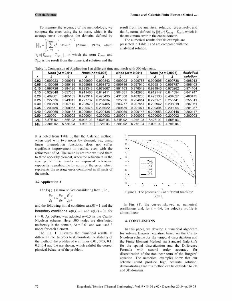
Table 1. Comparison of Application 1 at different time and mesh with 500 elements.

x Nnos (∆∆∆∆t = 0,01) Nnos (∆∆∆∆t = 0,005) Nnos (∆∆∆∆t = 0,001) Nnos (∆∆∆∆t = 0,0005) Analytical

solution 2 3 2 3 2 3 2 3

0.02 0.999923 0.999934 0.999999 0.999843 0.999992 0.999758 0.999995 0.999738 0.998913

0.05 0.100066 0.999136 0.999968 0.998472 0.999746 0.997910 0.999810 0.997787 0.996403

0.10 0.996726 0.984126 0.993343 0.979667 0.991163 0.976042 0.991945 0.975262 0.974164

0.15 0.929348 0.857383 0.911468 0.849411 0.904881 0.842986 0.912147 0.841394 0.841747

0.20 0.409301 0.465109 0.423914 0.475435 0.431388 0.483200 0.423133 0.484627 0.483475

0.25 0.227536 0.249012 0.227737 0.251834 0.225856 0.254814 0.223171 0.255741 0.255311

0.30 0.203609 0.207140 0.203570 0.207465 0.203277 0.207857 0.202942 0.208019 0.207961

0.35 0.200485 0.200983 0.200478 0.201022 0.200439 0.201071 0.200394 0.201094 0.201087

0.40 0.200065 0.200133 0.200064 0.200138 0.200059 0.200145 0.200053 0.200148 0.200147

0.50 0.200001 0.200002 0.200001 0.200002 0.200001 0.200002 0.200000 0.200002 0.200003

||||||||e||||||||2 8.87E-02 1.86E-02 6.99E-02 8.53E-03 6.51E-02 1.94E-03 7.42E-02 1.55E-03

||||||||e||||||||∞∞∞∞ 2.30E-02 5.53E-03 1.93E-02 2.72E-03 1.85E-02 6.27E-04 2.09E-02 4.79E-04

It is noted from Table 1, that the Galerkin method,

when used with two nodes by element, i.e., using

linear interpolation functions, does not suffer

significant improvement in results, even with the

refinement of ∆t. The same is not true we used them to three nodes by element, when the refinement in the

spacing of time results in improved outcomes,

especially regarding the L2 norm of the error, which represents the average error committed in all parts of

the mesh.

3.2 Application 2

The Eq.(1) is now solved considering Re=1, i.e.,

2

2

x

u

x

uu

t

u

∂

∂=

∂∂

+∂∂

and the following initial condition 1)0,( =xu and the

boundary conditions 1),0( =tu and 1,0),1( =tu for

t > 0. As before, was adopted α=0.5 in the Crank-Nicolson scheme. Here, 500 nodes are distributed

uniformly in the domain, ∆t = 0.01 and was used 3 nodes for each element.

The Fig. 1 illustrates the numerical results at different time. In order to demonstrate the stability of

the method, the profiles of u at times 0.01, 0.05, 0.1,

0.2, 0.4 and 0.6 are shown, which exhibit the correct

physical behavior of the problem.

Figure 1. The profiles of u at different times for

Re=1.

In Fig. (1), the curves showed no numerical

oscillations and, for t = 0.6, the velocity profile is

almost linear.

4. CONCLUSIONS

In this paper, we develop a numerical algorithm

for solving Burgers’ equation based on the Crank-

Nicolson scheme for the temporal discretization and

the Finite Element Method via Standard Galerkin's

for the spatial discretization and the Difference

Formula with second order accuracy for

discretization of the nonlinear term of the Burgers’

equation. The numerical examples show that our

scheme could produce high accurate solution,

demonstrating that this method can be extended to 2D

and 3D domains.



5. ACKNOWLEDGMENTS

The present work was supported by the National

Council of Scientific Development and Technology,

CNPq, Brazil (Proc. 500382/2011-5) and Mato

Grosso Research Foundation, Fapemat, Brazil (Proc.

292470/2010).

6. REFERENCES

Ali, A. H. A., Gardner, L. R. T. and Gardner, G.

A. (1992), A collocation method for Burgers’

equation using cubic splines, Computer Methods in

Applied Mechanics and Engineering, Vol. 100, pp.

325–337.

Chung, T. J., 2002, Computational Fluid

Dynamics, Cambridge University Press, Cambridge.

Dogan, A., 2004, A Galerkin finite element

approach to Burgers’ equation, Applied Mathematics

and Computation, Vol. 157, pp. 331-346.

Dag, I.; Irk, D. and Saka, B., 2005, A numerical

solution of the Burgers’ equation using cubic B-

splines, Applied Mathematics and Computation, Vol.

163, pp. 199-211.

Dhatt, G. and Touzout, G., 1984, The Finite

Element Method Displayed, John Wiley & Sons,

Chinchester.

Hoffmann, K. A. and Chiang S. T., 2000,

Computational Fluid Dynamics, 4th Ed., vol.I,

Engineering Education System, Wichita.

Guo-Zhong, Z.; Xi-Jun, Y. and Di, W., 2010,

Numerical solution of the Burgers’ equation by local

discontinuous Galerkin method, Applied

Mathematics and Computation, Vol. 216, pp. 3671–

3679.

Kevorkian, J., 1990, Partial Differential

Equations: Analytical Solution Techniques,

Wadsworth & Brooks/Cole Advanced Books &

Software, California.

Polyanin, A. D. and Zaitsev, V. F., 2004,

Handbook of Nonlinear Partial Differential

Equations, Chapman & Hall/CRC, Boca Raton.

Reddy, J. N., 1993, An Introduction to the Finite

Element Method, McGraw-Hill, Singapore.

Xu, M, Wang, R. H. and Qin Fang, J. H. Z.,

2011, A novel numerical scheme for solving

Burgers’ equation, Computers and Mathematics with

Application, Vol. 217, pp. 4473-4482.

Zhang, X. H., Ouyang, J. and Zhang, L., 2009,

Element-free characteristic Galerkin method for

Burgers’ equation, Engineering Analysis with

Boundary Elements, Vol. 33, pp. 356-362.

Zlhmal, M., 1978, Superconvergence and reduced

integration in the finite element method, Mathematics and Compututation, Vol.32, No.143, pp. 663-685.

galerkin finite element method and finite difference method for solving...

Documents