fuzzy special logic functions and applicationsfuzzy special logic functions and applications te-shun...

Florida International UniversityFIU Digital Commons

FIU Electronic Theses and Dissertations University Graduate School

3-31-1992

Fuzzy special logic functions and applicationsTe-Shun ChouFlorida International University

Follow this and additional works at: http://digitalcommons.fiu.edu/etd

Part of the Electrical and Computer Engineering Commons

This work is brought to you for free and open access by the University Graduate School at FIU Digital Commons. It has been accepted for inclusion inFIU Electronic Theses and Dissertations by an authorized administrator of FIU Digital Commons. For more information, please contact [email protected].

Recommended CitationChou, Te-Shun, "Fuzzy special logic functions and applications" (1992). FIU Electronic Theses and Dissertations. Paper 2347.http://digitalcommons.fiu.edu/etd/2347

http://digitalcommons.fiu.edu?utm_source=digitalcommons.fiu.edu%2Fetd%2F2347&utm_medium=PDF&utm_campaign=PDFCoverPages

http://digitalcommons.fiu.edu/etd?utm_source=digitalcommons.fiu.edu%2Fetd%2F2347&utm_medium=PDF&utm_campaign=PDFCoverPages

http://digitalcommons.fiu.edu/ugs?utm_source=digitalcommons.fiu.edu%2Fetd%2F2347&utm_medium=PDF&utm_campaign=PDFCoverPages

http://digitalcommons.fiu.edu/etd?utm_source=digitalcommons.fiu.edu%2Fetd%2F2347&utm_medium=PDF&utm_campaign=PDFCoverPages

http://network.bepress.com/hgg/discipline/266?utm_source=digitalcommons.fiu.edu%2Fetd%2F2347&utm_medium=PDF&utm_campaign=PDFCoverPages

http://digitalcommons.fiu.edu/etd/2347?utm_source=digitalcommons.fiu.edu%2Fetd%2F2347&utm_medium=PDF&utm_campaign=PDFCoverPages

mailto:[email protected]

ABSTRACT OF THE THESIS

Fuzzy Special Logic Functions and Applications

by

Te-Shun Chou

Florida International University, 1992

Miami, Florida

Professor Edward T. Lee, Major Professor

In this thesis, four special logic functions (threshold functions, monotone

increasing functions, monotone decreasing functions, and unate functions) are extended

to more general functions which allows the activities of these special functions to be a

"fuzzy" rather than a "1-or-O" process. These special logic functions are called as fuzzy

special logic functions and are based on the concepts and techniques developed in fuzzy

logic and fuzzy languages. The algorithms of determining C(n), Cm(n) and generating

the most dissimilar fuzzy special logic functions as well as important properties and

results are investigated. Examples are given to illustrated these special logic functions.

In addition, their applications -- function representation, data compression, error

correction, and monotone flash analog to digital converter, their relationships, and fuzzy

classification are also presented. It is obviously shown that fuzzy logic theory can be

used successfully on these four special logic functions in order to normalize the grade of

membership function p in the interval [0 1]. As a result, the techniques described in this

thesis may be of use in the study of other special logic functions and much fertile field

work is great worth researching and developing.

FLORIDA INTERNATIONAL UNIVERSITYMiami, Florida

Fuzzy Special Logic Functions and Applications

A thesis submitted in partial satisfaction of therequirements for the degree of Master of Science

in Electrical and Computer Engineering

by

Te-Shun Chou

1992

To Professors: Dr. Wunnava V. SubbaraoDr. Kang k. YenDr. Edward T. Lee

This thesis, having been approved in respect to form and mechanical execution, is referredto you for judgement upon its substantial merit.

Dean, Gordon R. HopkinsCollege of Engineering and Design

The thesis of Te-Shun Chou is approved.

Wunnava V. Subbarao

Kang k. Yen

Edward T. Lee, Major Professor

James R. Story, Chairman of Department of Electricaland Computer Engineering

Date of Examination: March 31, 1992

Dean, Richard CampbellDivision of Graduate Studies

Florida International University, 1992

ii

To

my parents

iii

ACKNOWLEDGEMENTS

I would like to acknowledge all who help in the completion of this thesis. First

of all, I had to thank all my committee members for their thorough reading of my thesis

as well as for their valuable advice and suggestions. Among them, I'd like to express my

gratitude to Dr. Kang K. Yen. He is so influential not only in my study, but also in my

life philosophy. Meanwhile, mostly I'd like to thank my major professor, Dr. Edward T.

Lee, whose influence on me is profound. I was very fortunate to have the opportunity

to learn with him. He provided me consistent help and advice, however the most

important is that he taught me how to view a problem in a different way and researched

it step by step. In a word, he is truly a good and helpful teacher.

In the meantime, I would be remiss if I did not mention my best friend, Mr. Ke-

Wen Zeng. He is a considerate person who always tried to help me in every way.

Thanks also to another good friend, Miss Ya-Fen Lee, who always supports and

encourages me both in my personal life and the completion of this thesis.

Furthermost, I would like to give my deepest gratitude to all my families,

especially my parents, P'eng-Hsiao Chou and Shiang-Lin W. Chou. They raised me with

all their hearts. Without their love and support, I could never have achieved my master

program. I want to share this wonderful honor with them. Again, thanks to them truly

from the bottom of my heart.

iv

Table of Contents

1. Fuzzy Threshold functions and Applications i

1.1 Introduction 1

1.2 Threshold functions (Linearly separable functions) 2

1.2.1 Properties of threshold gates 4

1.2.2 Advantages of threshold logic 5

1.3 Fuzzy threshold functions 8

1.4 Determination of pn 9

1.4.1 For two variables 9

1.4.2 For three variables 13

1.4.3 For n variables 16

1.4.4 Summary 17

1.5 An algorithm for determining Cm(n) 17

1.6 An algorithm for determining C(n) 18

1.7 An algorithm for generating most inseparable functions 23

1.8 Applications 25

1.8.1 Function representation 25

1.8.2 Data compression 26

1.8.3 Error detection and correction 26

1.9 Conclusion

2. Fuzzy Monotone functions and Applications

v

2.1 Introduction 28

2.2 Monotone increasing functions 28

2.3 Fuzzy monotone increasing functions 29

2.4 Determination of p. 30




2.4.4 Summary 33

2.5 An algorithm for determining C.m(n) 35


2.7 An algorithm for generating most variation functions 39

2.8 Monotone decreasing functions 41

2.9 Fuzzy monotone decreasing functions 41

2.10 Applications 43




2.10.4 Analog to digital converters 45

2.11 Conclusion 45

3. Fuzzy Unate functions and Applications 46

3.1 Introduction 46

3.2 Unate functions 46

vi

3.3 Fuzzy unate functions 47

3.4 Determination of p. 48




3.4.4 Summary 52

3.5 An algorithm for determining Cm(n) 54


3.7 An algorithm for generating most non-unate functions 59

3.8 Applications 60




3.9 Conclusion 62

4. Flash Analog to Digital Converters 63

4.1 Introduction 63

4.2 Basic structure 64

4.3 2-bit flash analog to digital converter 65



4.6 Conclusion 71

vii

5. Minimum Universal Synthesis of Logic Functions by Using

Monotone Flash Analog to Digital Converters 72

5.1 Introduction 72

5.2 Rule of choosing minterms or maxterms to synthesize a given function 72

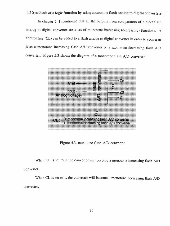
5.3 Synthesis of a logic function by using monotone flash A/D converters 76

5.3.1 Synthesis of a logic function by using monotone increasing

flash A/D converters 77

5.3.2 Synthesis of a logic function by using monotone decreasing

flash A/D converters 83

5.4 Conclusion 87

6. Fuzzy Classification 88

6.1 Introduction 88

6.2 Generalization 89

6.2.1 Fuzzy threshold functions 90

6.2.2 Fuzzy monotone functions 91

6.2.2 Fuzzy unate functions 91

6.3 Relationships 93

6.4 Classification %

6.5 Conclusion 99

7. Recommendations 1c

References 101

viii

Chapter One

Fuzzy Threshold Functions and Applications

1.1 Introduction

Digital computers, digital communication and control systems, and many other

digital systems deal with two general problems: the characterization of the input-output

relations of digital networks (using, for example, Boolean algebra), and the synthesis of

digital networks from their input-output relations using certain specified logic elements

as building blocks. Conventionally, these building blocks include such elements as AND,

OR, and NOR gates.

All of these conventional elements share two very useful properties: they are easily

constructed from standard components, and their input-output relations are simple and

easily described in Boolean algebra. However, since new circuit techniques now promise

the inexpensive mass fabrication of stable, reliable components, there is renewed interest

in using a logically more powerful basic building block -- the threshold gate and

McNaughton had the first published work in this field in 1957 [16]. Although this type

of gate requires tighter tolerances than conventional gates, it promises a substantial

reduction in the number of gates, the total number of components, and the number of

interconnections.

Therefore, I would like to discuss this subject and use the concepts and techniques

developed in fuzzy logic and fuzzy languages to fuzzify the kind of functions and their

some applications in this chapter.

1

1.2 Threshold functions fT (Linearly separable functions)

A threshold gate which is a logic device with n binary-valued inputs, x, x2 , ... , x,

and a single binary-valued output y. Associated with each input xi is a weight w;. The

values of the threshold T and wi (i=1, 2,..., n) may be any real, finite, positive or negative

numbers. The output y of the threshold gate is decided by as follows [9,15,16]:

[1.1]y =1 i f and cnly if ( W1 x 1 2T

1=1

[1.2]y =O i f and only i ff wx < T

1=1

where the sum and product operations are arithmetic. A threshold gate is represented

pictorially as shown in Figure 1.1.

X

Figure 1.1. The symbol of a threshold gate

Clearly, a threshold gate realizes a Boolean function. Hence, the output of a

threshold gate can be represented by a Boolean function as definition 1.1.

2

DEFINITION 1.1. [15,16] A threshold function is defined as:

[1.3]y =( ( w~x1 4,

1=1

where equation 1.3 is called the threshold function representation of the gate.

DEFINITION 1.2. A function is an inseparable function while it is not a threshold

function.

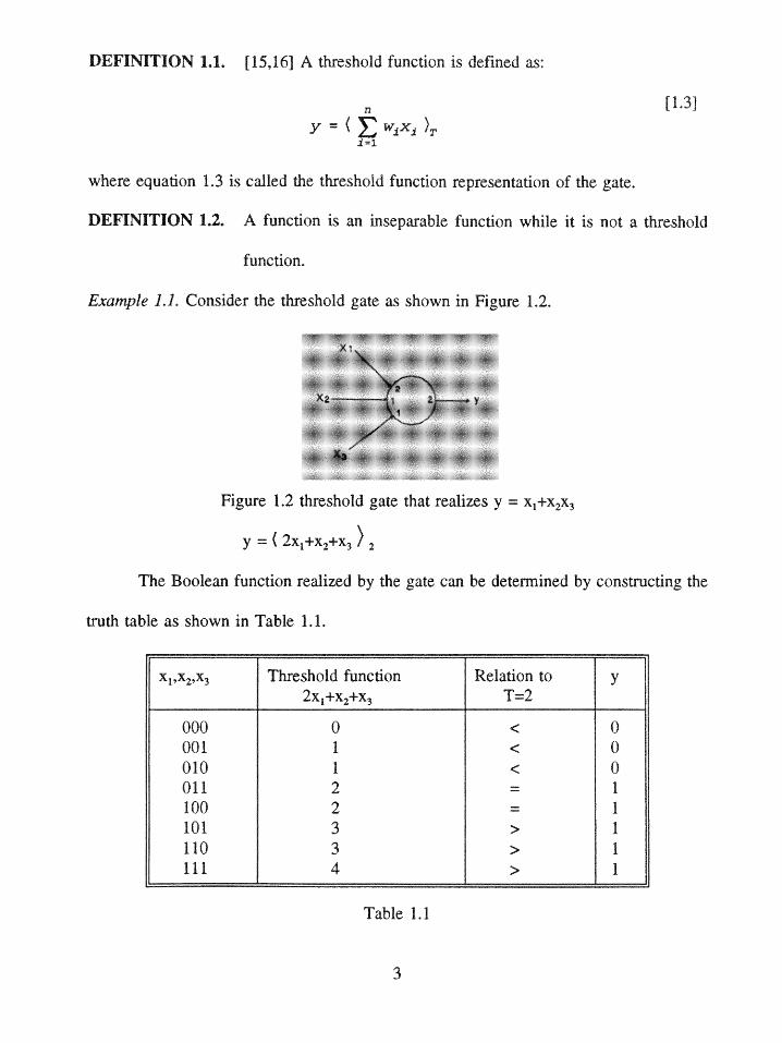
Example 1.1. Consider the threshold gate as shown in Figure 1.2.

Figure 1.2 threshold gate that realizes y = x1+x 2x3

y = ( 2x1+x 2+x 3 2

The Boolean function realized by the gate can be determined by constructing the

truth table as shown in Table 1.1.

x x2 x3 Threshold function Relation to y2x1+x 2+x 3 T=2

000 0 0001 1 < 0010 1 < 0011 2 - 1100 2 1101 3 1110 3 1111 4 1

Table 1.1

3

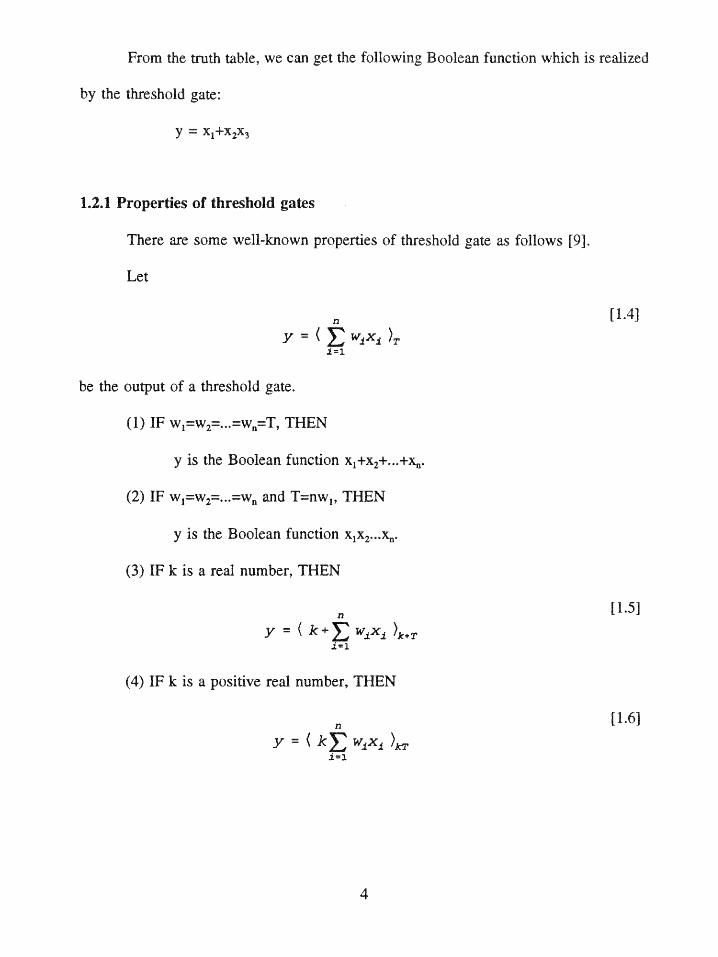
From the truth table, we can get the following Boolean function which is realized

by the threshold gate:

y = x1+x 2x 3

1.2.1 Properties of threshold gates

There are some well-known properties of threshold gate as follows [9].

Let

[1.4]

i=1

be the output of a threshold gate.

(1) IF wl=w2=...=wg=T, THEN

y is the Boolean function xl+x2+...+x.

(2) IF w,=w2=...=wn and T=nw,, THEN

y is the Boolean function xlx2.- xn-

(3) IF k is a real number, THEN

[1.5]y = ( k+( W1x 1 )k+

s=1

(4) IF k is a positive real number, THEN

[1,6]

_y =_X ) wxi=1

4

(5) IF k is a positive real number, THEN

[1.7]y!= ( -( w~x1 )

i=1

Example 1.2. Using property 1, a threshold gate realization of a three-variable OR is

given below:

x1+x2+X3 = ( x1+x 2+x3 )

Example 1.3. Using property 2, a threshold gate realization of a three-variable AND is

as follows:

x 1x 2x 3 = ( x 1+x 2+x 3 ) 3

Example 1.4. Property 3 is useful for changing the signs of coefficients.

y = ( -2x 1-x 2+x 3 ) -1

Determine an equivalent realization that only requires positive weights.

That is x,=1-xj'. Then:

y = ( -2(1-x 1')-(1-x 2')+x 3 ) 4

= ( -2+2x 1'-1+x 2 '+x 3 ) -1

= ( -3+2x1 '+x 2'+x 3 ) -1

= ( 3-3+2x1'-1+x 2'+x3 ) 31

= ( 2x 1'+x 2'+x 3 ) 2

1.2.2 Advantages of threshold logic

THEOREM 1.1. [9] A threshold gate for which all weights have unit value and the

threshold value is 0.5 is a n-input OR gate.

5

Example 1.5. For a two-variable function which satisfies theorem 1.1.

XIX 2 x+x 2 y= (xI+x 2 O.500 0 001 1 110 1 111 1 1

After calculation, we have found this threshold gate is equal to a 2-input OR gate.

THEOREM 1.2. [9] A threshold gate for which all weights have unity value and the

threshold value is n-0.5 is a n-input AND gate.

Example 1.6. For a two-variable function which satisfies theorem 1.2.

xx 2 xx 2 y =( xIx2) 0.5

00 0 001 0 010 0 011 1 1

After calculation, we found this threshold gate is equal to a 2-input AND gate.

THEOREM 1.3. [9] In a similar situation, the complementing threshold gate is a

generalization of the NOR and NAND gates.

Because of the wide range of possible weights and threshold values, the size and

complexity of the class of logical functions that can be realized by a single threshold gate

are large when compared with those of the conventional logical elements. As a result,

the number of gates, inputs, and total number of physical components needed to realize

a particular logical function are smaller for threshold gates than for conventional gates.

6

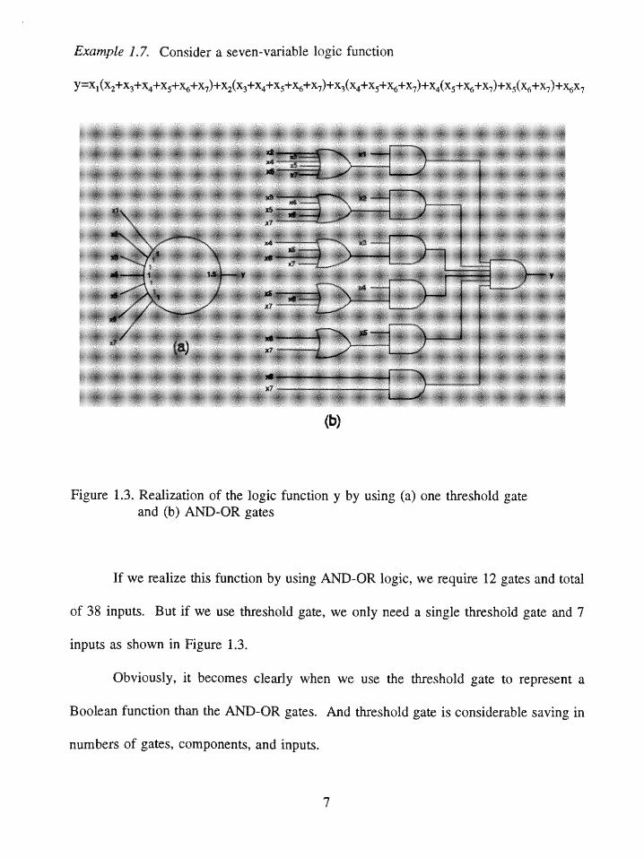
Example 1.7. Consider a seven-variable logic function

y=xl(x2+x3+x4+x5+ +x7)+x2(x3+x4+x5+6+x7)+x3( +x5+ +x7)+ 4( + +x7)+xs( +x7)+x,67

x2~

x8

()

(b)

Figure 1.3. Realization of the logic function y by using (a) one threshold gateand (b) AND-OR gates

If we realize this function by using AND-OR logic, we require 12 gates and total

of 38 inputs. But if we use threshold gate, we only need a single threshold gate and 7

inputs as shown in Figure 1.3.

Obviously, it becomes clearly when we use the threshold gate to represent a

Boolean function than the AND-OR gates. And threshold gate is considerable saving in

numbers of gates, components, and inputs.

7

1.3 Fuzzy threshold functions

Fuzzy threshold functions can be defined using the concepts and techniques

developed in fuzzy logic and fuzzy languages.

DEFINITION 1.3. [5,13] The grade of membership function of a fuzzy threshold

function f is defined to be:

p ) = [1.8]

where C is the minimum number of minterms change in order to convert f to be a

threshold function and p is a normalization constant which will be discussed in later

sections.

LEMMA 1.1. For all threshold functions fT,

C(f) o [1.9]

p'T(fT) = [1.10]

pT(fT)=1 indicates that f has full membership in the class of threshold functions.

LEMMA 1.2. For all functions f of n variables, an upper bound for C is:

[1.11]C(n) No. of total minters

2

8) 12

C8 <2

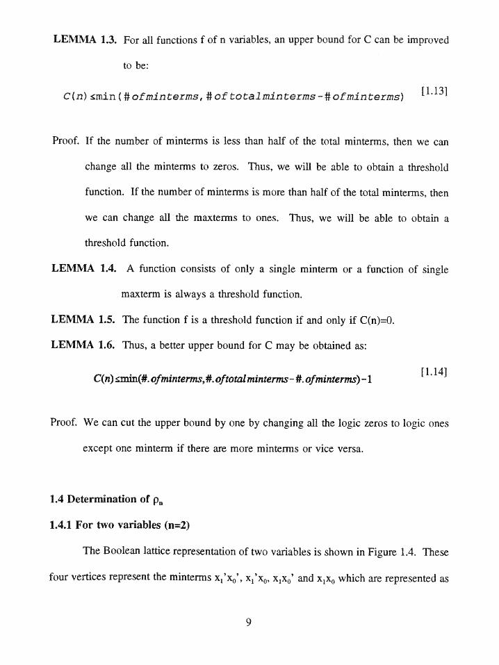
LEMMA 1.3. For all functions f of n variables, an upper bound for C can be improved

to be:

C(n) Amin (#ofrminterms, #oftotal interms -# ofminterms) [1.13]

Proof. If the number of minterms is less than half of the total minterms, then we can

change all the minterms to zeros. Thus, we will be able to obtain a threshold

function. If the number of minterms is more than half of the total minterms, then

we can change all the maxterms to ones. Thus, we will be able to obtain a

threshold function.

LEMMA 1.4. A function consists of only a single minterm or a function of single

maxterm is always a threshold function.

LEMMA 1.5. The function f is a threshold function if and only if C(n)=O.

LEMMA 1.6. Thus, a better upper bound for C may be obtained as:

C(n) min(#. ofminterms,#. oftotalminterms- #.ofminterms)-1 1.14]

Proof. We can cut the upper bound by one by changing all the logic zeros to logic ones

except one minterm if there are more minterms or vice versa.

1.4 Determination of pn

1.4.1 For two variables (n=2)

The Boolean lattice representation of two variables is shown in Figure 1.4. These

four vertices represent the minterms xl'xo', x1 'xO, xjxO' and xjxO which are represented as

9

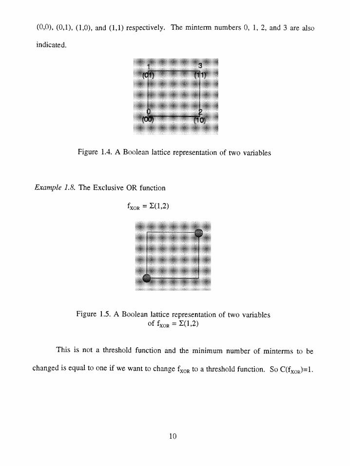
(0,0), (0,1), (1,0), and (1,1) respectively. The mintermr numbers 0, 1, 2, and 3 are also

indicated.

Figure 1.4. A Boolea lattice representation of wo variables

Example 1.8. The Exclusive OR function

fxoR = XMl,2

Figure 1.5. A Boolean lattice representation of two variablesof = XoR = ) ,

This is not a threshold function and the minimum number of minterms to be

changed is equal to one if we want to change fxOR to a threshold function. So C(fxoR)=l.

10

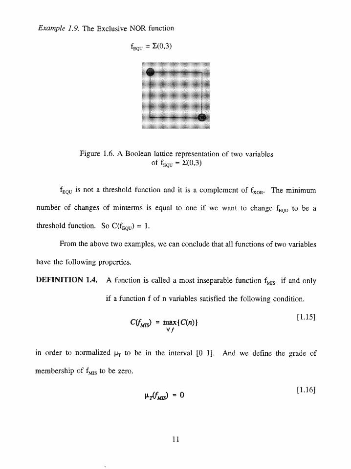
Example 1.9. The Exclusive NOR function

fEQu (0,)

Figure 1.6. A Boolean lattice representation of two variablesof fEQU (0,)

fEQU is not a threshold function and it is a complement of fxOR. The minimum

number of changes of minterms is equal to one if we want to change fEQU to be a

threshold function. So C(fEQU) = 1*

From the above two examples, we can conclude that all functions of two variables

have the following properties.

DEFINITION 1.4. A function is called a most inseparable function f s if and only

if a function f of n variables satisfied the following condition.

C(fMIs) = max{C(n)} [1.15]

Vf

in order to normalized pT to be in the interval [0 1]. And we define the grade of

membership of f s to be zero.

pIff Is) = o [1.16]

11

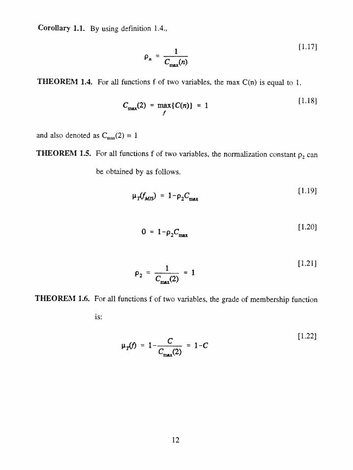
Corollary 1.1. By using definition 1.4,

[1.17]1

THEOREM 1.4. For all functions f of two variables, the max C(n) is equal to 1.

C.(2) = max{C(n)} = 1 [1.18]f

and also denoted as Cm(2) = 1

THEOREM 1.5. For all functions f of two variables, the normalization constant P2 can

be obtained by as follows.

p1fM0) = 1-p 2C. [1.19]

o = 1-p 2 C. [1.20]

1 [1.21]

C.(2)

THEOREM 1.6. For all functions f of two variables, the grade of membership function

is:

[1.22]pg)= 1---= 1-C

Cm(2)

12

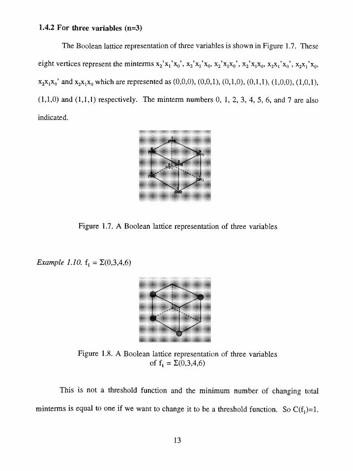
1.4.2 For three variables (n=3)

The Boolean lattice representation of three variables is shown in Figure 1.7. These

eight vertices represent the minterms x2 'xi'x ', x2'x1 'x0, x2 'x1X 0', X2'x1x 0 , x 2X 1'X0 ', X2X1'x0,

x 2 X1XO' and x 2 x1x0 which are represented as (0,0,0), (0,0,1), (0,1,0), (0,1,1), (1,0,0), (1,0,1),

(1,1,0) and (1,1,1) respectively. The minterm numbers 0, 1, 2, 3, 4, 5, 6, and 7 are also

indicated.

Figure 1.. A Boolean lattice representation of three variables

Example 1.10. f, = X(0,3,4,6)

Figure 1.8. A Boolean lattice representation of three variablesof f1 = (0,3,4,6)

This is not a threshold function and the minimum number of changing total

minterms is equal to one if we want to change it to be a threshold function. So C(fl)=1.

13

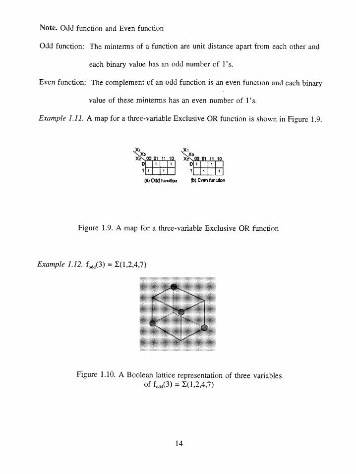
Note. Odd function and Even function

Odd function: The minterms of a function are unit distance apart from each other and

each binary value has an odd number of l's.

Even function: The complement of an odd function is an even function and each binary

value of these minterms has an even number of l's.

Example 1.11. A map for a three-variable Exclusive OR function is shown in Figure 1.9.

x x1

(a) Odd fundon ) Even fun don

Figure 1.9. A map for a three-variable Exclusive OR function

Example 1.12. fod(3) = (1,2,4,7)

Figure 1.10. A Boolean lattice representation of three variablesof fodd(3) = I(1,2,4,7)

14

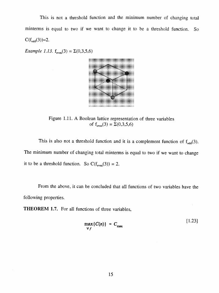
This is not a threshold function and the minimum number of changing total

rinterms is equal to two if we want to change it to be a threshold function. So

C(fedd(3))=2.

Example 1.13. f v (3) = (0,3,5,6)

Figure 1.11. A Boolean lattice representation of three variablesof feven(3) = (0,3,5,6)

This is also not a threshold function and it is a complement function of f (3 ).

The minimum number of changing total minterms is equal to two if we want to change

it to be a threshold function. So C(fe(3)) = 2.

From the above, it can be concluded that all functions of two variables have the

following properties.

THEOREM 1.7. For all functions of three variables,

max{C(n)} [1.23]

15

THEOREM 1.8. For all functions f of three variables, the normalization constant p3 can


C.(3) = 2 [1.24]

= 1p 3 C. [1.25]

o = 1-p 3C. [1.26]

[1.27]

C.(3) 2

THEOREM 1.9. For all functions of three variables, the grade of membership function

is:

[1.28]C C

C.(3) 2

1.4.3 For n variables

THEOREM 1.10. From the derivation of two and three variables, we can generalize the

grade of membership function for n variables as:

[1.29]=1 C

C.(n)

16

1.4.4 Summary

From above theorems and examples, we can summarize the results in Table 1.2

and derive an algorithm for determining Cm(n), an algorithm for determining C(n), and

an algorithm for generating most inseparable functions of subsequent sections.

No. of No. of most most membership possiblevariables C inseparable inseparable function values

functions functions of PT

2 1 2 (0,3) P(f)=1-C 0,1(1,2)

3 2 2 X(0,3,5,6) pT(f)=1-C/2 0,1/2,11(1,2,4,7)

Table 1.2. Summary of two and three variables functions

1.5 An algorithm for determining C..(fn)

After the derivations of two and three variables, we can determine Cm(n) for n

variables by using the same method.

THEOREM 1.11. For all functions of n variables with n 4,

C.(n) = 2'-'1 [1.30]

THEOREM 1.12. For all member of variables, the number of most inseparable functions

are always equal to 2.

THEOREM 1.13. The function f is a threshold function if and only if f' is a threshold

function, This theorem can be generalized to fuzzy threshold

functions.

17

THEOREM 1.14. For all functions f of n variables, then

C) =C)[1.31]

[1.32]

1.6 An algorithm for determining C(n)

Boolean lattice and Karnaugh map are both common ways to represent logic

functions. So we replace Boolean lattice by using Karnaugh map to do the algorithm for

determining C(n) in this section.

We limit our presentation in two and three variables here and it is the same

approach while above three variables.

We can convert one representation to the other by using Figures 1.12 and 1.13.

X 1O

Figure 1.12. The two-variable map from Boolean latticerepresentation to Karnaugh map

18

Txx ii

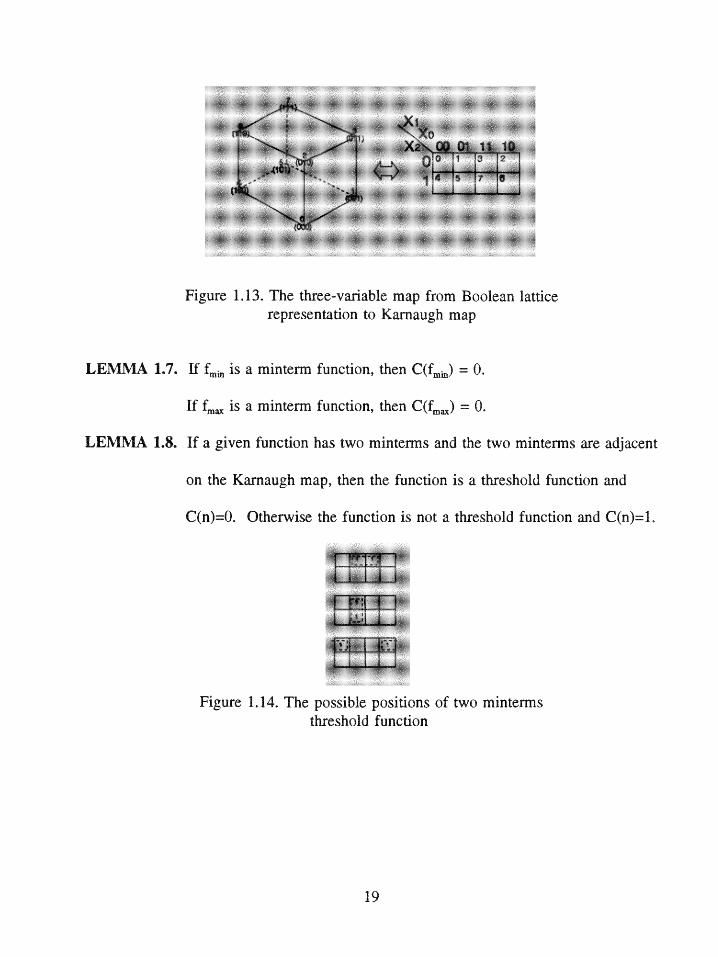
Figure 1.13. The three-variable map from Boolean latticerepresentation to Karnaugh map

LEMMA 1.7. f.,, is a minterm function, then C(fmj,) = 0.

If f. is a minterm function, then C(f ) = 0.

LEMMA 1.8. If a given function has two minterms and the two minterms are adjacent

on the Karnaugh map, then the function is a threshold function and

C(n)=0. Otherwise the function is not a threshold function and C(n)=1.

Figure 1.14. The possible positions of two mintermsthreshold function

19

Example 1.14. A threshold function: f = X(,1)

A fuzzy threshold function: f = X(2,5)

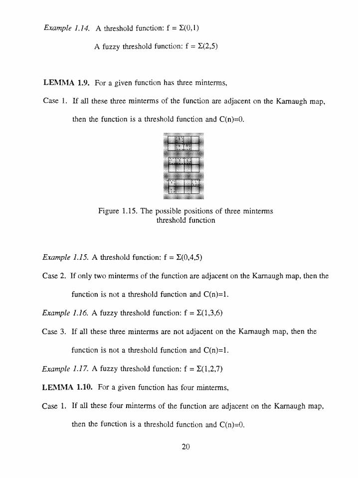
LEMMA 1.9. For a given function has three minterms,

Case 1. If all these three minterms of the function are adjacent on the Karnaugh map,

then the function is a threshold function and C(n)=O.

Figure 1.15. The possible positions of three mintermsthreshold function

Example 1.15. A threshold function: f = X(0,4,5)

Case 2. If only two minterms of the function are adjacent on the Karnaugh map, then the

function is not a threshold function and C(n)=l.

Example 1.16. A fuzzy threshold function: f = X(1,3,6)

Case 3. If all these three minterms are not adjacent on the Karnaugh map, then the

function is not a threshold function and C(n)=l.

Example 1.17. A fuzzy threshold function: f = (1,2,7)

LEMMA 1.10. For a given function has four minterms,

Case 1. If all these four minterms of the function are adjacent on the Karnaugh map,

then the function is a threshold function and C(n)=O.

20

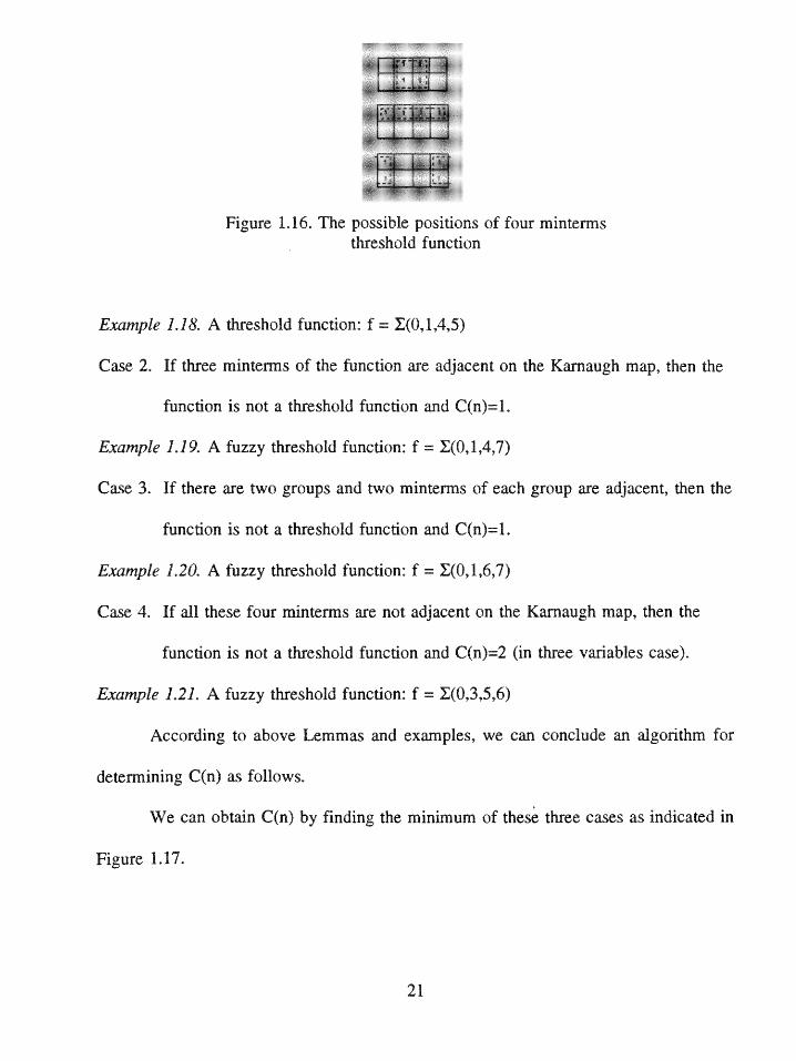
Figure 1.16. The possible positions of four mintermsthreshold function

Example 1.18. A threshold function: f = X(0,1,4,5)

Case 2. If three minterms of the function are adjacent on the Karnaugh map, then the

function is not a threshold function and C(n)=1.

Example 1.19. A fuzzy threshold function: f = X(0,1,4,7)

Case 3. If there are two groups and two minterms of each group are adjacent, then the

function is not a threshold function and C(n)=1.

Example 1.20. A fuzzy threshold function: f = I(0,1,6,7)

Case 4. If all these four minterms are not adjacent on the Karnaugh map, then the

function is not a threshold function and C(n)=2 (in three variables case).

Example 1.21. A fuzzy threshold function: f = X(0,3,5,6)

According to above Lemmas and examples, we can conclude an algorithm for

determining C(n) as follows.

We can obtain C(n) by finding the minimum of these three cases as indicated in

Figure 1.17.

21

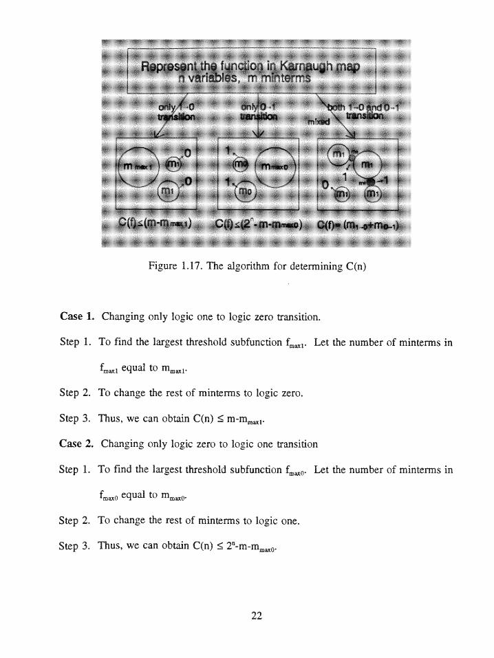
Represent the function in Karnaugh mapS variables,tr minterms

onl h, - on 0 1-0 end -1

Figure 1.17.T algorithm for determining C(n)

Case 1. Changing only logic one to logic zero transition.

Step 1. To find the largest threshold subfunction fm0 . Let the number of minterms in

fm a equal to , .

Step 2. To change the rest of minterms to logic zero.

Step 3. Thus, we can obtain C(n) < mm O.

Case 2. Changing only logic zero to logic one transition

Step 1. To find the largest threshold subfunction fffiO. Let the number of minterms in

f~aO equal to m O.

Step 2. To change the rest of mintrs to logic one.

Step 3.Tus, we can obtain C(n) 2"-m- O.

22

Case 3. Changing some minterms to logic zero and some maxterms to logic one in order

to connect all the subfunctions. Thus, we can obtain C(n) =

At last, we can combine these three cases and then obtain the minimum C(n).

C(n) = min[(m -m,),(2"-m-m ),(m1 +m )] [1.33]

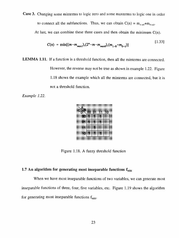
LEMMA 1.11. If a function is a threshold function, then all the minterms are connected.

However, the reverse may not be true as shown in example 1.22. Figure

1.18 shows the example which all the minterms are connected, but it is

not a threshold function.

Example 1.22.

D-\00 10

i I

Figure 1.18. A fuzzy threshold function

1.7 An algorithm for generating most inseparable functions fus

When we have most inseparable functions of two variables, we can generate most

inseparable functions of three, four, five variables, etc. Figure 1.19 shows the algorithm

for generating most inseparable functions f s.

23

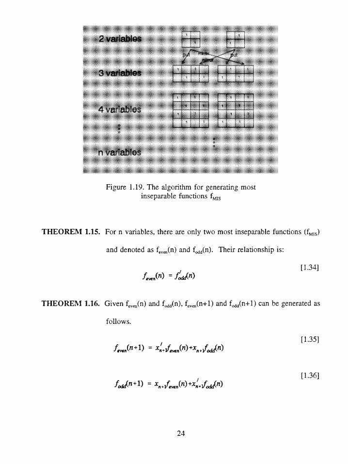
3 variables

4variables

**nvariables

Figure 1.19. The algorithm for generating mostinseparable functions fu

THEOREM 1.15. For n variables, there are only two most inseparable functions (f s)

and denoted as f,,(n) and fod(n). Their relationship is:

[1.341f.(n) = f n) [3

THEOREM 1.16. Given fe(n) and fed(n), fe,,(n+l) and fed(n+1) can be generated as

follows.

f,.(n+1) =x.f ()x. n)[3]

[1.36]fnn+l) =x ,

24

1.8 Applications

Fuzzy threshold functions can be applied to function representation, data reduction,

and error correction. The results may have useful applications to logic design, pattern

recognition, and related areas.

1.8.1 Function representation

Fuzzy threshold functions can be used as a tool to represent any logic function f.

If C(n) = i, then

f = fy G (m,m 2 >,m) [1.37]

fy= f G (m,m 2,...,m) [1.38]

where fT is a threshold function, G indicates the exclusive-or operation and i 1 , i 2,..., m ;

are minterms which should be changed from fT in order to obtain f.

Usually, this representation is not unique. In other word, there may exist f'T such

that:

f = f'. G E(m ,n,...,m ) [1.39]

Example 1.23. f = X(0,3,5,6) is an inseparable function with C(f)=2, it can be represented

as f = I(0,2,3,6)G (m2 ,m,) or f = I(0,1,3,5)GX(mi,m6 ) where X(0,2,3,6) and 1(0,1,3,5)

both are threshold functions.

25

1.8.2 Data compression

A threshold function can be represented [w1 ,w2,...,w.;T] which has a simpler

representation compare with a general logic function.

For function f with C(n)=1, then function f can be represented by:

f = fT tm} 1.40]

Thus, for transmitting f, instead of transmitting the total truth table or the

corresponding Kamaugh map, we can transmit only fT and the minterms mi. Therefore,

data compression may be achieved.

1.8.3 Error detection and correction

Fuzzy threshold functions also can be applied to error detection. For example, if

we know that a most inseparable function (fs) is transmitted and a single error occurred,

then at the receiving end,

~ [1.41]

where f' indicates the function received.

We know that there are only two most inseparable functions for n variables.

Therefore, if we transmit a most inseparable function of n variables, then all the single

error can be detected and corrected. Actually, the capability of error correction is

stronger than when single error occurred.

26

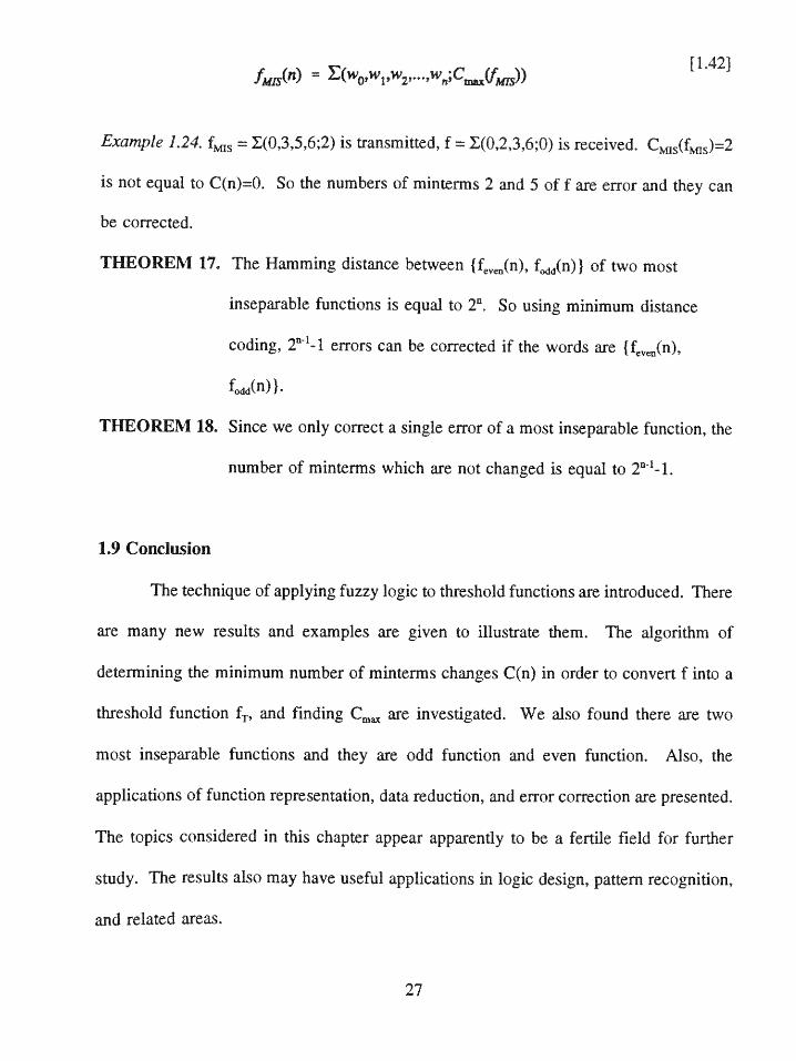
fj(n) = L Y , 1,42]))

Example 1.24. f s = X(0,3,5,6;2) is transmitted, f = X(0,2,3,6;0) is received. Cas(f s)=2

is not equal to C(n)=0. So the numbers of minterms 2 and 5 of f are error and they can

be corrected.

THEOREM 17. The Hamming distance between {f(ven), f(dd(n)} of two most

inseparable functions is equal to 2". So using minimum distance

coding, 2n-11 errors can be corrected if the words are {fve(n),

faddn).

THEOREM 18. Since we only correct a single error of a most inseparable function, the

number of minterms which are not changed is equal to 2"--1.

1.9 Conclusion

The technique of applying fuzzy logic to threshold functions are introduced. There

are many new results and examples are given to illustrate them. The algorithm of

determining the minimum number of minterms changes C(n) in order to convert f into a

threshold function fT, and finding C. are investigated. We also found there are two

most inseparable functions and they are odd function and even function. Also, the

applications of function representation, data reduction, and error correction are presented.

The topics considered in this chapter appear apparently to be a fertile field for further

study. The results also may have useful applications in logic design, pattern recognition,

and related areas.

27

Chapter Two

Fuzzy Monotone Functions and Applications

2.1 Introduction

Monotone functions play an important role in switching theory, logic design,

computer design, flash analog to digital converter, pattern classification, and pattern

recognition. In particular, flash analog to digital converter is designed using the set of

all monotone increasing (decreasing) functions. The details shall be discussed in chapter

4 and 5.

In this chapter, 1 will introduce fuzzy monotone functions which are using the

concepts and techniques developed in fuzzy logic and fuzzy languages.

2.2 Monotone increasing functions fame

DEFINITION 2.1. [9,15] A Boolean function f of n variables is monotone increasing

if and only if xsy implies that f(x)<f(y), where x=(x1,x 2,--.,xa) and

y=(yIy 2,--.,yn) and x, x2,.., x, Y11 y2 -.., y are either "logic zero"

or "logic one".

THEOREM 2.1. [9,15] For a function which is n variables, there are 2"+1 monotone

increasing functions. More specifically, they are shown in Table

2.1.

28

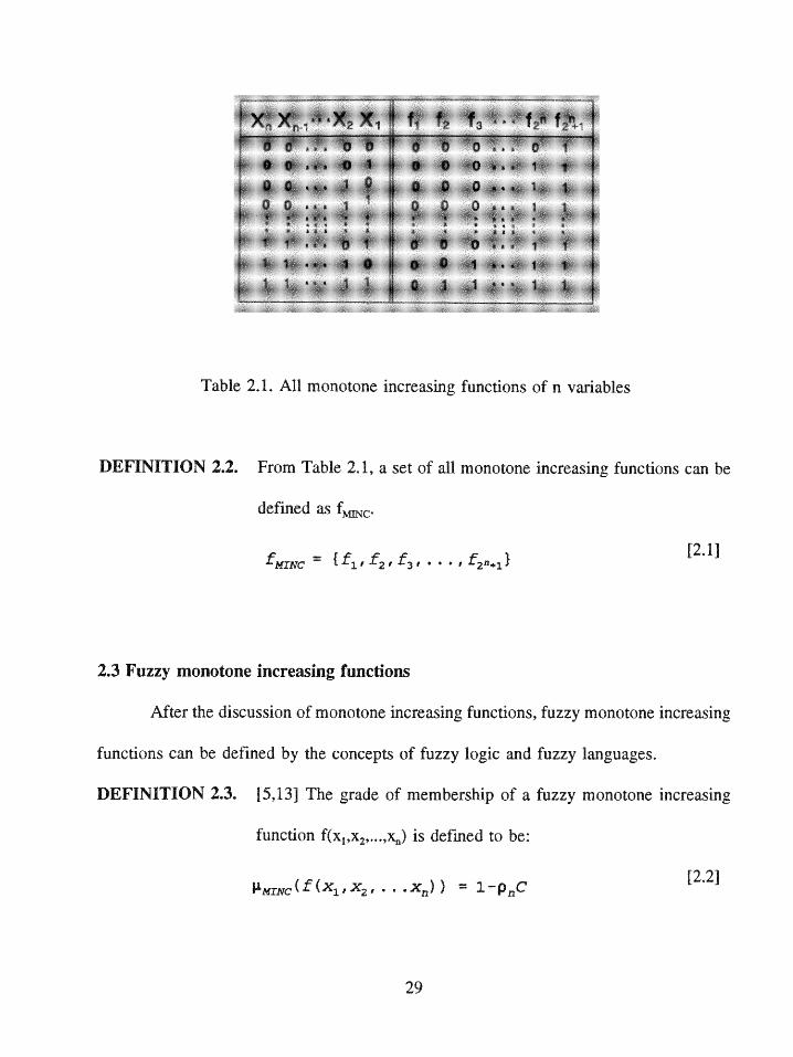
Table... 2..A-mntn nraigfntoso aibeXfi Xs f 1 t n

pMN iC 3p o " I"+Table2F1zAll monotone increasing funco fDEIIIN22 Fro Tabl 2. se of 1 mootn inrasn fucin ca bedefne as

2.3l FuzzyAl monotone increasing functions o aibe

After the discussion of monotone increasing functions, fuzzy monotone increasing

functions can be defined by the concepts of fuzzy logic and fuzzy languages.

DEFINITION 2.3. [5,13] The grade of membership of a fuzzy monotone increasing

function f(xl,x2,--,xi) is defined to be:

INC fXl x 2 ,3 . . . [ 2.

29

where C is the minimum number of minterms change in order to convert f(xl,x2,...,x) to

be a monotone increasing function (a member in f c) and p. is a normalization constant

which will be determined in section 2.4.

LEMMA 2.1. For a monotone increasing function f(x,x 2 ,...,x ), the minimum number

of minte s change is equal to:

C(xf I X2 x) = o [2.3]

LEMMA 2.2. For a monotone increasing function f(x1,x 2 ...,x ), f(x1,x 2,.,x1 ) has full

membership in the class of monotone functions and indicates as:

IpMrNC 1~x, X2 , ... ,x) Xn[4

And we normalize kme in the interval [0 1].


According to Table 1, for all monotone increasing functions, if we scan the output

column from the top to the bottom, there is only one change of truth value from 0 to 1.

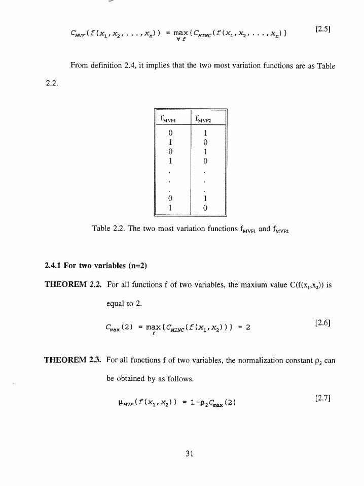
DEFINITION 2.4. Thus, we define that the function is most dissimilar to monotone

increasing functions to be the most variation function fMVF which

has the following property, that is, if we scan the output column

from the top to the bottom, there will be most number of changes

of truth value from 0 to 1.

30

avr~ (f X1, 2 - - - -x,,) -= mx "IC c. f (.x,,2' , .... X) ['2

From definition 2.4, it implies that the two most variation functions are as Table

2.2.

f1 i MVF2

0 11 0o 11 0

o 11 0

Table 2.2. The two most variation functions fMVF1 d MVF2


THEOREM 2.2. For all functions f of two variables, the maxium value C(f(x1,x 2)) is

equal to 2.

C.( 2) = max {CMINC fx, X2 ) ) I = 2[26if

THEOREM 2.3. For all functions f of two variables, the normalization constant p2 can


p=l (f x, )) 1- 2 C (2) [2.7]

31

o = 1-p 2 C (2) [2.

P2 1 [2.9]


is:

I)C 1 [2.10]

p YINC fxl,x) X2 C(2


THEOREM 2.5. For all functions f of three variables, the normalization constant p, can


C.(3) = 4 [2.11]

I, x, 3 = 1-p 3CM(3) [2.12]

o = 1-p C.(3) [2.13]

1 1 [2.14]

THEOREM 2.6. For all function of three variables, the grade of membership function

is:

32

INC ,X 2 ,X 3 C[2.15]


THEOREM 2.7. From above derivation, for all functions f of n variables can be

generalized as:

C. (n) = 2n-1 [2.16]

rC [2 .17]

[2.18]

2.4.4 Summary

From above theorems and examples, the results can be summarized as following

theorems, and tables. Furthermore, the algorithm for determining Cm(n) and C(n), and

the algorithm for generating most variation functions are also can be achieved by using

these results.

For any two and three-variable functions, the results can be summarized as Table

2.3.

33

No. of No. of most most membership possiblevariables C. variation variation function v ues

functions functions of pkiNC

A(0,2) p cf2 2 2 X(1,3) = 1-(C/2) 0,1/2,1

X(0,2,4,6) p0c(f) 4,1/4,2/4

3 4 2 X(1,3,5,7) = 1-(C/4) ,3/4,1

Table 2.3. Summary of two and three-variable functions

THEOREM 2.8. The number of monotone increasing function (fc) is 2"+1.

And it can be summarized as shown in Table 2.4.

number of variables number of f

2 5

3 9

4 17

5 33

n 2n+l

Table 2.4. Summary of fc of n variables

LEMMA 2.3. A function of constant "logic zeros" or constant "logic ones" is a

monotone increasing function.

34

Example 2.1. For a function of three variables, then f=(0,1,2,3,4,5,6,7) and

f=1(0,1,2,3,4,5,6,7) are two monotone increasing functions.

THEOREM 2.9. Given two functions f1 and f2 which both are monotone increasing

functions of n variables, then f 1 - c is a monotone increasing

function which is equal to the smaller one.

Example 2.2. Two functions fmc =X(5,6,7) and f21 c=X(4,5,6,7) which both are

monotone increasing functions of three variables , then f 1 - c is a monotone

increasing function which is equal to the smaller one f1c=(5,6,7).

THEOREM 2.10. Given two functions fi and f2 which both are monotone increasing

functions of n variables, then f1 c+f2 c is a monotone increasing

function which is equal to the larger one.

Example 2.3. Two functions f l =(5,6,7) and f2mc= (4,5,6,7) which both are

monotone increasing functions of three variables , then f1 c+f2 c is a monotone

increasing function which is equal to the larger one f2mc=(4,5,6,7).

2.5 An algorithm for determining Cm(f)

THEOREM 2.11. For all functions of two variables, Cm(2) = 2

THEOREM 2.12. For all functions of three variables, Cm(3) = 4

THEOREM 2.13. For all functions of n variables,

Ci(n) = 2~1 [2.19]

And it can be summarized as shown in Table 2.5.

35

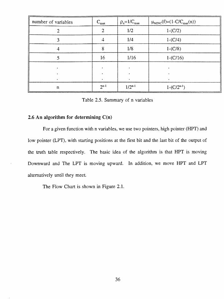
number of variables Cp =n1/Cax c(f)=(1-C/C (n))

2 1/2 1-(C/2)

4 1/4 1(C/4)

8 1/8 1-(C/8)

5 16 1/16 1-(C/16)

n 2 n11/2" n-C/"

Table 2.5. Summary of n variables


For a given function with n variables, we use two pointers, high pointer (HPT) and

low pointer (LPT), with starting positions at the first bit and the last bit of the output of

the truth table respectively. The basic idea of the algorithm is that HPT is moving

Downward and The LPT is moving upward. In addition, we move HPT and LPT

alternatively until they meet.

The Flow Chart is shown in Figure 2.1.

36

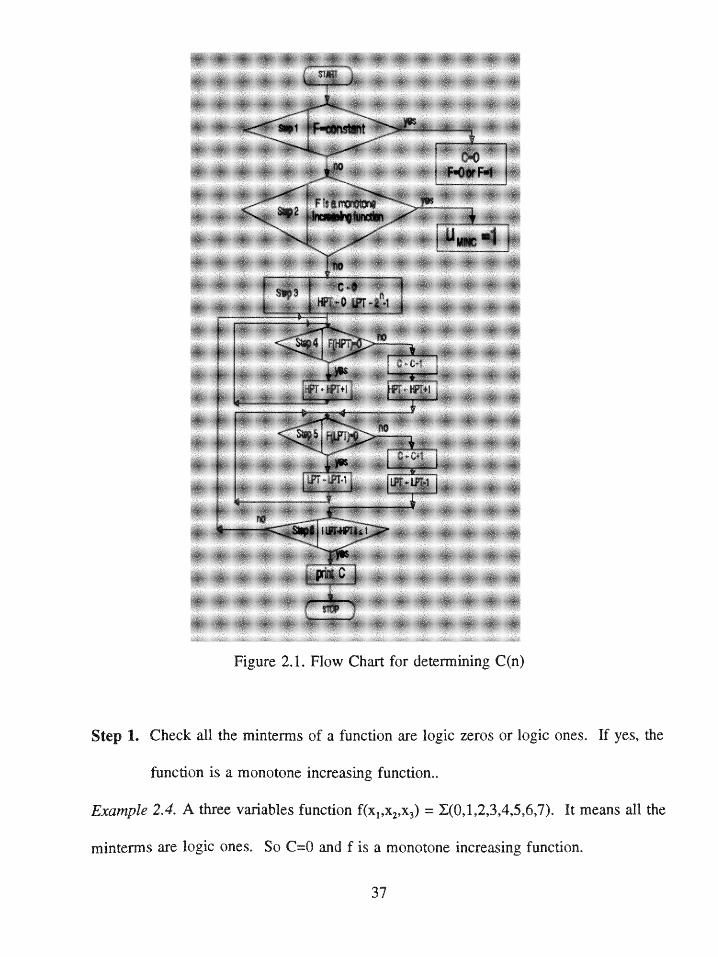
ggp F ¬of u

* R~I

Step L Check all the minte of afuctio) r oiczrso lgcoe.fys hP -LPT1 r..PT.1

Figure 2.1. Flow Chart for determining C(n)

Step 1.Check all the minterms of a function are logic zeros or logic ones. Ifyes, the

function is a monotone increasing function..

Example 2.4. A three variables function f(x1 ,x 2,x 3) = X(Ol,2,3,4,5,6,7). It means all the

minterms are logic ones. So C=O and f is a monotone increasing function.

37

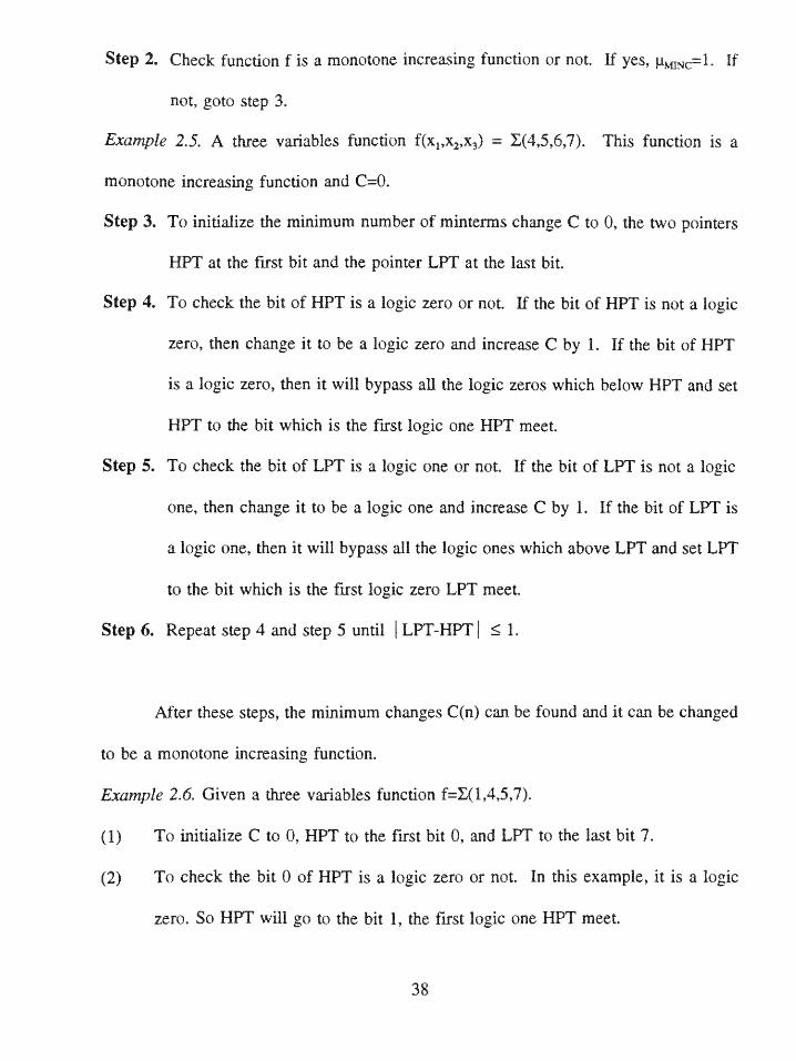
Step 2. Check function f is a monotone increasing function or not. If yes, paMIc=l If

not, goto step 3.

Example 2.5. A three variables function f(x1 ,x2 ,x 3) = Y(4,5,6,7). This function is a

monotone increasing function and C=0.

Step 3. To initialize the minimum number of minterms change C to 0, the two pointers

HPT at the first bit and the pointer LPT at the last bit.

Step 4. To check the bit of HPT is a logic zero or not. If the bit of HPT is not a logic

zero, then change it to be a logic zero and increase C by 1. If the bit of HPT

is a logic zero, then it will bypass all the logic zeros which below HPT and set

HPT to the bit which is the first logic one HPT meet.

Step 5. To check the bit of LPT is a logic one or not. If the bit of LPT is not a logic

one, then change it to be a logic one and increase C by 1. If the bit of LPT is

a logic one, then it will bypass all the logic ones which above LPT and set LPT

to the bit which is the first logic zero LPT meet.

Step 6. Repeat step 4 and step 5 until I LPT-HPT :5 1.

After these steps, the minimum changes C(n) can be found and it can be changed

to be a monotone increasing function.

Example 2.6. Given a three variables function f=m(l,4,5,7).

(1) To initialize C to 0, HPT to the first bit 0, and LPT to the last bit 7.

(2) To check the bit 0 of HPT is a logic zero or not. In this example, it is a logic

zero. So HPT will go to the bit 1, the first logic one HPT meet.

38

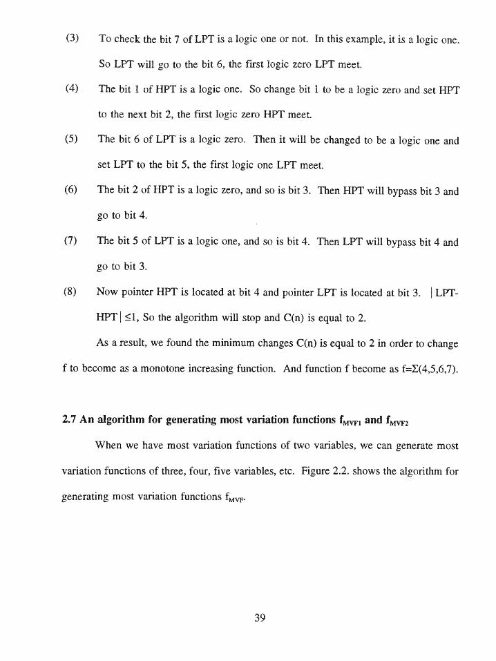
(3) To check the bit 7 of LPT is a logic one or not. In this example, it is a logic one.

So LPT will go to the bit 6, the first logic zero LPT meet.

(4) The bit 1 of HPT is a logic one. So change bit 1 to be a logic zero and set HPT

to the next bit 2, the first logic zero HPT meet.

(5) The bit 6 of LPT is a logic zero. Then it will be changed to be a logic one and

set LPT to the bit 5, the first logic one LPT meet.

(6) The bit 2 of HPT is a logic zero, and so is bit 3. Then HPT will bypass bit 3 and

go to bit 4.

(7) The bit 5 of LPT is a logic one, and so is bit 4. Then LPT will bypass bit 4 and

go to bit 3.

(8) Now pointer HPT is located at bit 4 and pointer LPT is located at bit 3. LPT-

HPT :51, So the algorithm will stop and C(n) is equal to 2.

As a result, we found the minimum changes C(n) is equal to 2 in order to change

f to become as a monotone increasing function. And function f become as f=X(4,5,6,7).

2.7 An algorithm for generating most variation functions fmw1 and f 2

When we have most variation functions of two variables, we can generate most

variation functions of three, four, five variables, etc. Figure 2.2. shows the algorithm for

generating most variation functions fMVF'

39

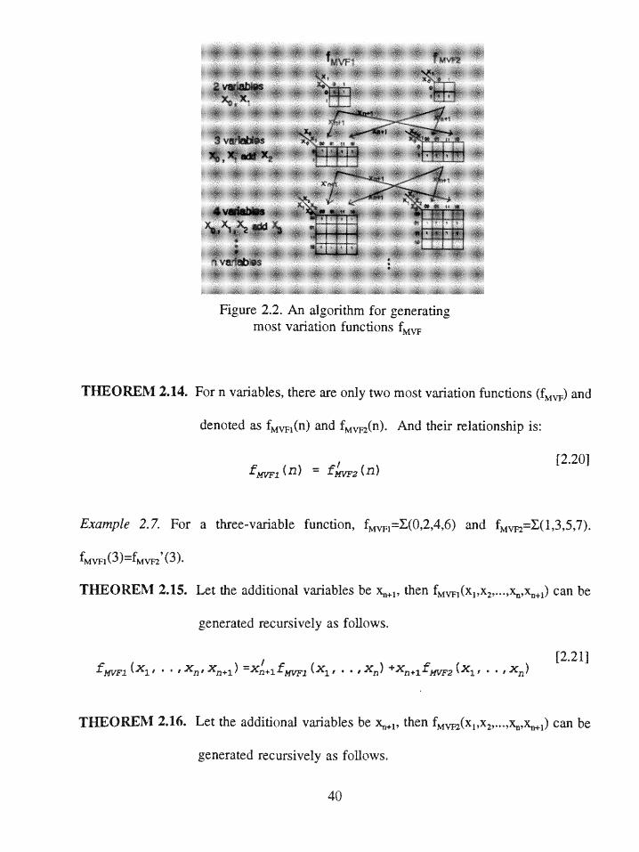
Figure 2.2. Anagorithm for generatigmost variation functions M

THEOREM 2.14. For n variables, there are only two mnost variation functions (fMVF) and

denoted as fMVFn)an fMVF(n). And their relationship is:

[2.20]

Example 2.7. For a three-variable function, fMVFX(, 2 4 6 )an Mvr2=X(l,3,5,7).fMVF MFF Y

THEOREM 2.15. Let the additional variables be X, then fM xlx 2 ,XngX.+l) can be

generated recursively as follows.MVF21, .. , n te f1 =n1V2 , .a , Xn), And their reaiosi i ,

THEOREM 2.16. Let the additional variables be X.1, then fMV(XX 2,...X,xX l) can be

generated recursively as follows.

40

,MVF2 I, ., , Xn 1 ) fXn+lSvF1(X, ,X) +x lfMF 2 (x ,, x X 2,221

2.8 Monotone decreasing functions fMDEc

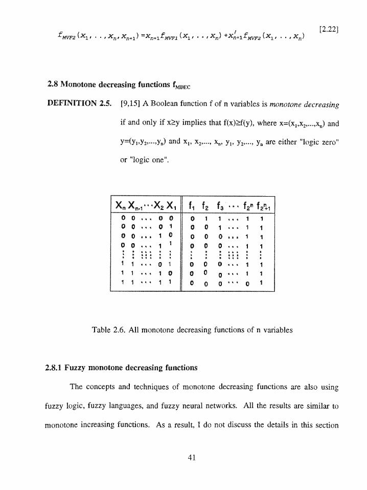
DEFINITION 2.5. [9,15] A Boolean function f of n variables is monotone decreasing

if and only if xy implies that f(x) f(y), where x=(x 1,x2,-.,xn) and

y= (y,y2,---,yn) and x, x2 ,.-, xn= Y1 Y2,---, yn are either "logic zero"

or "logic one".

X -X, <X 2 X1 f, f2 f - fr f2 100 ,, 00 0 1 1 , 1 1o 0 ,, 0 1 0 0 1 , , 1 1

0 0a.a1 0 0 0 Oa,.. 1 I

S 00 0 .1 1

mootn inceain fucios a reut la o o 'ics eti'ti eto1 1 at, 0 1 0 0 0 ,, 1 11 1 ,,, 1 0 0 0 0 ,,, 1 1

1 1 a'' 1 1 0 0 0 ,'' 0 1

Table 2.6. All monotone decreasing functions of n variables

2.8.1 Fuzzy mnonotone decreasing functions

The concepts and techniques of monotone decreasing functions are also using

fuzzy logic, fuzzy languages, and fuzzy neural networks. All the results are similar to

monotone increasing functions. As a result, I do not discuss the details in this section

41

again and only write down the important results here.

Fuzzy monotone decreasing functions is also defined using the concept of fuzzy

logic and fuzzy languages.

EC ix, X 2 , ... ,x) n 123

where we normalize pMEc in the interval [0 1 and PMDEC = 1 for all the monotone

decreasing functions.

THEOREM 2.17. For all function of n variables, the number of monotone decreasing

functions (fDEC) is equal to 2n+1.

THEOREM 2.18. For all function f of n variables, the number of maximum number of

minterms changes (Cm) in order to become as a monotone

decreasing functions (fEc) is equal to 2 .

So the membership function becomes as:

C C [2.24]LMDEC (n)_

THEOREM 2.19. The two most variation functions fMVF1 andM are the same as those

of monotone increasing functions.

The algorithm for deterining C(n) is similar to the one of monotone increasing

functions except HPT is checking the bit is logic one or not and LPT is checking logic

zero or not.

42

2.9 Applications

Fuzzy monotone increasing functions can be applied to switching theory, logic

design, computer design, flash analog to digital converter, pattern classification, pattern

recognition, and pattern understanding. In particular, flash analog to digital converter is

designed using the set of all monotone increasing (decreasing) functions.


Fuzzy monotone increasing functions can be used as a tool to represent any logic

function f.

If C(n) = i, then

_ ~ MINC 1 2rn" r " ' ) [2.25]

where f c is a monotone increasing function, e indicates the exclusive or operation and

i 1 , i 2 ,..., m1 are minterms which should be changed from f c in order to obtain f.

Example 2.8. If we want to convert f(x1,x 2 ,x 3) = X(1,3,4,6,7) into a monotone increasing

function faC(x,x 2 ,x 3), 'then C(f(x,x 2 ,x 3))=2 and it can be represented as f(x,,x 2,x 3) =

X(3,4,5,6,7)GX(m ,m).


A monotone increasing function can be represented [wI,w 2,...,w,;C] which has a

43

simpler representation compare with a general logic function,

For function f with C(n)=i, then function f can be represented by

f = fmINvC ,,[,7


corresponding Karnaugh map, we can transmit only fumc and the minterms m;. Therefore,



Fuzzy monotone increasing functions also can be applied to error detection. For

example, if we know that a most variation function (fMF) is transmitted and errors

occurred, then at the receiving end,

C .; ) [2.28]

where 'MVF indicates the function received.

We know that there are only two most variation functions for n variables.

Therefore, if we transmit a most variation function of n variables, then all the errors can

be detected and corrected.

Example 2.9. fMF(xl,x2 ,x3 ) = (1,3,5,7;C=4) is transmitted, f(x1 ,x2,x 3) = X(4,5,6,7;C=O)

is received. C(fMF(xlx 2,x 3))=4 is not equal to C(f(XIX 2,X 3))=0. So the numbers of

minterms I, 3, 4, and 6 of f are erroneous and they can be corrected.

44

2.9.4 Analog to digital converter

Given a n-bit flash converter input an analog signal, we can get 2" digital outputs

after 2'-1 comparators. Since these 2" digital outputs are all monotone increasing

(decreasing) functions, any function can be represented by the combinations of these

monotone increasing (decreasing) functions. These details and results shall be discussed

and presented in chapter 4 and 5.

2.10 Conclusion

Fuzzy monotone functions are introduced, investigated by using the concepts and

techniques which developing in fuzzy logic and applied to function representation, data

compression, error correction, and monotone flash analog to digital converter. The

algorithm for determining C(n), Cm(n) and generating the most variation functions fMMF1

and fMVF2 are presented. Examples are given to illustrated this fuzzy special function.

The are many results and they may be have useful applications in logic design, pattern


45

Chapter Three

Fuzzy Unate Functions and Applications

3.1 Introduction

After the introduction of threshold functions and monotone functions, my principal

goal in this chapter is the development of methods for another special logic functions,

unate functions, which also play an important role in switching theory, logic design,

computer design, pattern classification, and pattern recognition.

Also, fuzzy unate functions are introduced using the concepts and techniques

developed in fuzzy logic and fuzzy languages and also applied to function representation,

data compression, and error detection.

3.2 Unate functions u

DEFINITION 3.1. [21] A function f(x1 ,x2,p.-,x ) is said to be positive in a variable x,

if there exists a disjunctive or conjunctive expression for the

function in which x; appears only in uncomplemented form.

DEFINITION 3.2. [21] Analogously, f(xl,x 2,-,,xn) is said to be negative in a variable

x, if there exists a disjunctive or conjunctive expression for the

function in which x, appears only in complemented form.

DEFINITION 3.3. [21] Derived from definition 3.1 and 3.2, if a Boolean function

f(xJx 2,...,xn) is either positive or negative in xi, it means that there

is no variable appears both uncomplemented and complemented

46

when f is written in a minimum sum of products form, then

function f(xI,x2,---,xn) is said to be unate in x, and f is a unate

function.

Example 3.1. The following are both unate functions:

f(x 1,x2,x 3) = x 1+x 2x 3

f2(x 1,x 2,x3) = X1'X2'+X3'

Proof: All the variables of fl function or f2 appear no both uncomplemented and

complemented. So both functions fl and f2 are unate functions.

Example 3.2. On the other hand, the following functions are not unate:

f 3(x1,x 2,x 3) = x 1x2+x,'x2'x 3

f 4(x 1,x2,x 3) = x 1x2'+x 2x 3

Proof: Variables x1 and x 2 of function f 3 and variable x 2 of function f4 appear both

uncomplemented and complemented. So both functions f3 and f4 are not unate.

3.3 Fuzzy unate functions

Fuzzy unate functions can be defined using the concepts and techniques developed

in fuzzy logic and fuzzy languages.

DEFINITION 3.4. [5,13] The grade of membership of a fuzzy unate function

f(x1,x 2,...,x.) is defined to be:

p x x 1 I -lg1oXn) ) = 1-nC [3.1]

where C is the minimum number of minterms change in order to convert f(x1,x 2,---,xn) to

47

be a unate function (a member in fu) and p. is a normalization constant which will be

determined in later sections.

LEMMA 3.1. For a unate function f(xl,x2,..,x ), the minimum number of minterms

change is equal to:

C(f(x 1x 2x, . .,x) = o [3.2]

LEMMA 3.2. For a unate function f(xl,x2,.-.,x ), f(x1,x2,.-,x ) has full membership in the

class of unate functions and indicates as:

pg(f (x 1 , x 2 ,., x -K) ) = 1 [3.3]

And we normalize pu in the interval [0 1].



Example 3.3. The Exclusive OR function

fxOR = (1,2)

xoXi 0 1

0 1

1 1

fxoR =xo*x = xo'x 1+xox 1', From definition 3.3, if there is no variable appears

48

both uncomplemented and complemented when f is written in a minimum sum of

products form, then function f(xI,x 2,.-,x ) is said to be unate in x; and f is a unate

function. Now variables x0 and x, appear both uncomplemented and complemented. So

this is not a unate function and the

minimum number of minterms to be changed is equal to one in order to change the

function fXoR to be a unate function. C(fxoR) = 1.

Example 3.4. The Exclusive NOR function

EQU (,3)

xi 0 101

1 1

fEQU = xo x, = x0 +x 0'xl'. Using the same definition, variables x 0 and x, appear

both uncomplemented and complemented now. So this is not a unate function and the

minimum number of minterms to be changed is equal to one in order to change the

function fEQU to be a unate function. C(fEQU) = 1.

From example 3.1 and 3.2, we can conclude the following theorems.

THEOREM 3.1. For all functions f of two variables, the max value C(f(x,x 2)) is equal

to 1.

)= max{C(f(xx 2 ) ) = 1 [3.4]

49

THEOREM 3.2. For all functions f of two variables, the normalization constant p2 can


pm(f,(x 1 x 2 ) ) = 1-p 2 (2) [3.5]

0 = 1-p 2 C (2) [3.6]

1 =[3.7]Cax(2)


is:

[3.8]Ciax (2)


Example 3.5. fed(3) = (l,2,4,7)

X1Xo

X2 00 01 11 100 1 1

fod( 3 ) = x 0Gxpex 2 = xOxI'x 2 '+xo'xlx 2 '+xo'x'x 2+xoxix 2. Variables x0, xj, and x2 all

appear uncomplemented and complemented now. So fed( 3 ) is not a unate function and

the minimum number of minterms to be changed is equal to one in order to change it to

50

be a unate function. C(f,,( 3)) = 1.

Example 3.6. feven(3) = (0,3,5,6)

X1Xo

X2 00 01 11 1001 1

1 1 1

feven( 3 ) = xOoxIox2 = xo'xi'x 2'+xoxix 2 '+xOxI'x 2+xO'xIx2 . Variables x, xj, and x 2 all

appear uncomplemented and complemented now. So this function is not a unate function

and the minimum number of minterms to be changed is equal to one in order to change

fev (3) to be a unate function. C(feven(3)) = 1.

From above, we can conclude all three-variable functions have the following

properties.

THEOREM 3.4. For all functions f of three variables, the normalization constant p3 can


Cm (3) = 2 [3.9]

p.( (x1, x2r X3 ) = 1~-p3 Cma (3) [3.10]

o = 1-p2C.(3) [3.11]

[3.12]

3 C (3) 2

51

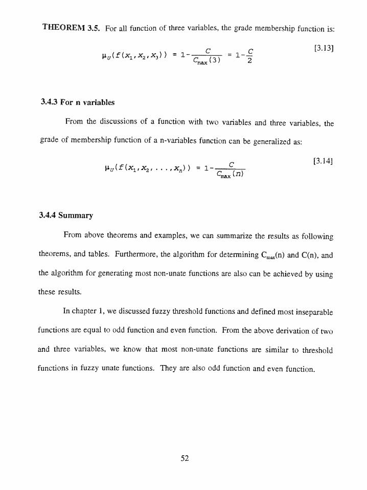
THEOREM 3.5. For all function of three variables, the grade membership function is:

f x x I) Xc 3 c [3 13]


From the discussions of a function with two variables and three variables, the

grade of membership function of a n-variables function can be generalized as:

,x)) ~ c[3.14]p ( f (x"~z -s - n )=)

3.4.4 Summary

From above theorems and examples, we can summarize the results as following

theorems, and tables. Furthermore, the algorithm for determining Cm.(n) and C(n), and

the algorithm for generating most non-unate functions are also can be achieved by using

these results.

In chapter 1, we discussed fuzzy threshold functions and defined most inseparable

functions are equal to odd function and even function. From the above derivation of two

and three variables, we know that most non-unate functions are similar to threshold

functions in fuzzy unate functions. They are also odd function and even function.

52

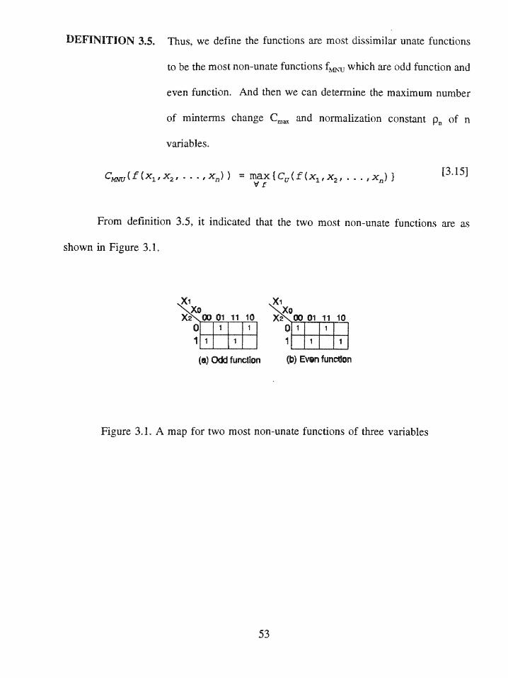
DEFINITION 3.5. Thus, we define the functions are most dissimilar unate functions

to be the most non-unate functions f which are odd function and

even function. And then we can determine the maximum number

of minterms change C.m and normalization constant p, of n

variables.

CMU( f (Ix1, --- x))= max{IC,( f(xx,' n [3.15]1ff

From definition 3.5, it indicated that the two most non-unate functions are as

shown in Figure 3.1.

X1 X1Xo Xo

X2 00 0111 10 X2 000 11 100 1 1 0 1 1

(a) Odd function (b) Even functon

Figure 3.1. A map for two most non-unate functions of three variables

53

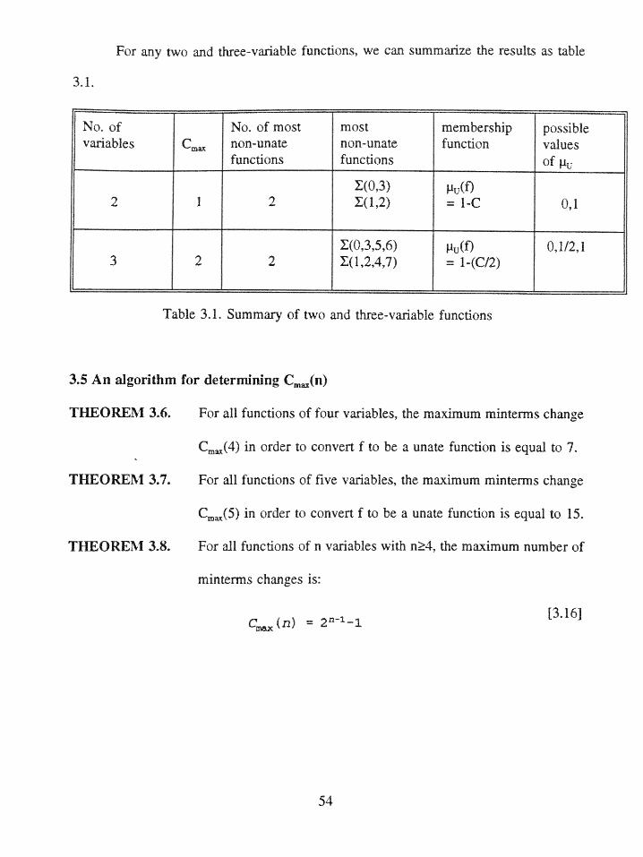
For any two and three-variable functions, we can summarize the results as table

3.1.

No. of No. of most most membership possiblevariables Cm non-unate non-unate function values

functions functions of

(0,3) p(2 1 2 (1,2) = 1-C 0,1

(0,3,5,6) Pu( 0,1/2,13 2 2 (1,2,4,7) = 1-(C/2)

Table 3.1. Summary of two and three-variable functions

3.5 An algorithm for determining Cm(f)

THEOREM 3.6. For all functions of four variables, the maximum minterms change

Cm.( 4 ) in order to convert f to be a unate function is equal to 7.

THEOREM 3.7. For all functions of five variables, the maximum minterms change

Cm (5) in order to convert f to be a unate function is equal to 15.

THEOREM 3.8. For all functions of n variables with n 4, the maximum number of

minterms changes is:

C. (n) = 2"11 [3.16]

54

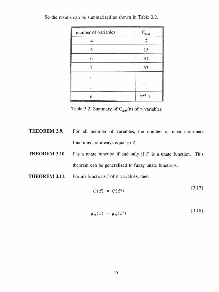
So the results can be summarized as shown in Table 3.2.

number of variables C.

4 7

5 15

6 31

7 63

n 2n 1-l

Table 3.2. Summary of Cm(fn) of n variables

THEOREM 3.9. For all member of variables, the number of most non-unate

functions are always equal to 2.

THEOREM 3.10. f is a unate function if and only if f' is a unate function. This

theorem can be generalized to fuzzy unate functions.

THEOREM 3.11. For all functions f of n variables, then

C(f) = C(f') [3.17]

(f) = (f) [3.18]

55


In this section, we can also use Boolean lattice representation (chapter 1) to help

us determining a function is whether a unate function or not. So I would like to explain

the Boolean lattice representation again because we will use some terminologies here.

An n-variable Boolean lattice representation contains 2" vertices, each of which

represents an assignment of values to the n variables and thus corresponds to a minterm.

A line is drawn between every pair of vertices which differ in just one variable, and no

other lines are drawn. The vertices corresponding to true minterms, that is, for which the

function assumes the value logic one, are called true vertices, while those corresponding

to false minterms are called false vertices.

THEOREM 3.12. [21] A logic function f(x1,x2 ,...,x ) is unate if and only if it is not

tautology and partial ordering exists, so that for every pair of

vertices (a1,a2,...,a) and (b ,b2 ,...,b ), if (a1,a2,...,an) is a true vertex

and (bl,b2,...,b) > (al,a,...,a), then (b1,b2,...,bn) is also a true vertex

of f.

Note. Partial orderin set of vertices is a lattice and the vertices (O,0,...,0) and (1,1,...,1)

are, respectively, the least vertex and the greatest vertex of the lattice.

According to theorem 3.12, a procedure can be written in order to change any n-

variable function into a unate function and to decide the minimum number of minterms

change.

56

Step 1. To find all the subcubes' minterms and minimal true vertices of each subcube.

Step 2. To check partial ordering relation of every subcube.

If yes, the function is a unate function.

If not, change the minterms which does not satisfy the partial ordering relation.

Step 3. To determine the number of minterms change.

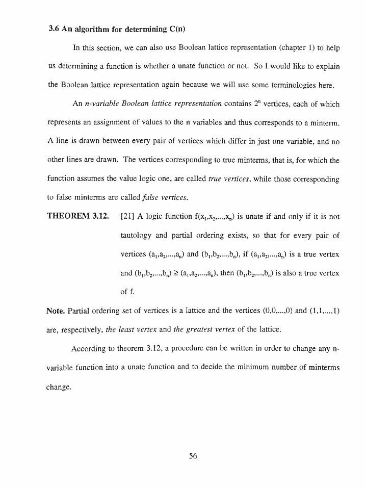
Example 3.7. For a function fl(x1,x 2 ,x 3) = x 1'x 2'+xlx 3 and the three-variable Boolean

lattice representation is shown in Figure 3.2.

Figure 3.2. The Boolean lattice representation of f1(x1 ,x 2 ,x 3 ) = xi'x 2 '+xlx 3

Step 1. There are two pairs of vertices [(0,0,1) and (0,0,0), (1,1,1) and (1,0,1)] and we

name the two minimal true vertices are S,=(0,0,0) and S2=(1,0,1).

Step 2. According to partition ordering, once the least vertex (0,0,0) is logic one, then all

the others vertices should be true vertices. But the vertices (1,0,0), (0,1,0), (0,1,1), and

(1,1,0) are not true vertices now. So we change the least vertex (0,0,0) to false vertex

and minterm (0,0,1) becomes as a minimal true vertex.

Step 3. To check the partial ordering relation of these two subcubes. We found (0,1,1)

57

is not a true vertex which true vertex (0,0,1) is not covered by it. So we have to change

(0,1,1) to be a true vertex.

Step 4. From the above steps, we found that we changed two vertices, (0,0,0) and (0,1,1),

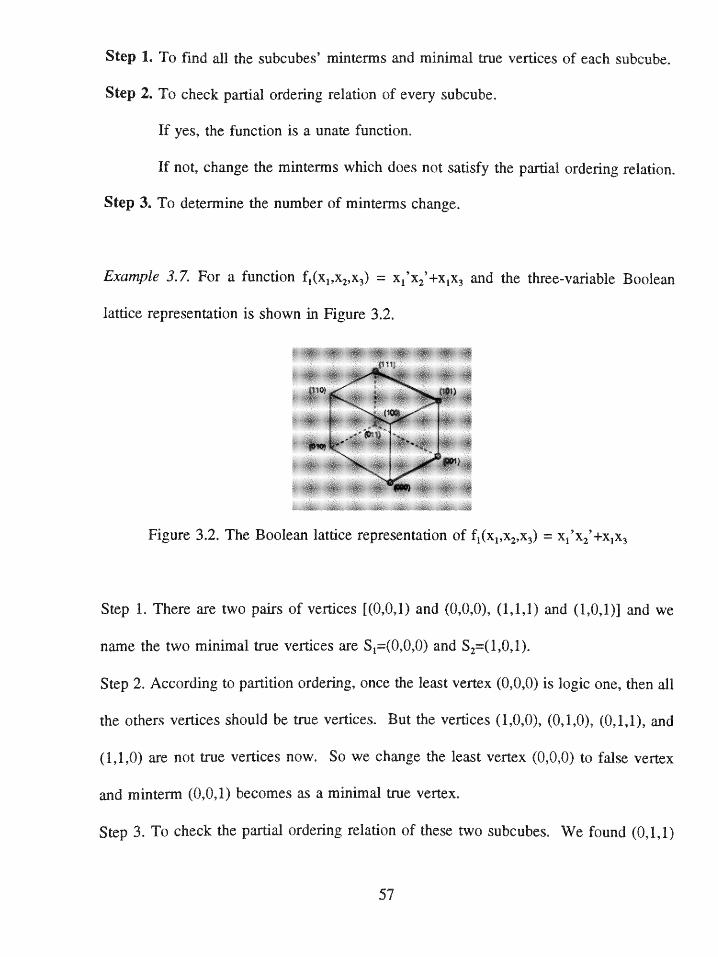
and f, becomes as a unate function - fl(x 1,x2,x3) = x 1'x 3+x1 x3 = x3 and C(n) is equal to

2. The Boolean lattice representation is shown in Figure 3.3.

Figure 3.3. The Boolean lattice representation of f1(x1,x 2,x3) = x1'x 3'+x1x =x3

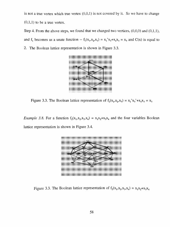
Example 3.8. For a function f2 (x 1,x 2 ,x 3,x 4 ) = x 1x2+x 3x 4 and the four variables Boolean

lattice representation is shown in Figure 3.4.

Figure 3.3. The Boolean lattice representation of f2(x1 x2,x3,x4) = x1x2+x3x4

58

Step 1. There are two pairs of vertices [(1,1,0,0), (1,1,1,0), (1,1,0,1), and (1,1,1,1),

(0,0,1,1), (1,0,1,1), (0,1,1,1), and (1,1,1,1)] and we name the two minimal true vertices

are S1=(0,0,1,1) and S2=(1,1,0,0).

Step 2. To check the partial ordering relation of these two subcubes. We found that every

vertex are greater than S, and S2.

Step 3. From the above steps, we can say that f 2 is a unate function and the number of

minterms change C(n) is equal to 0.

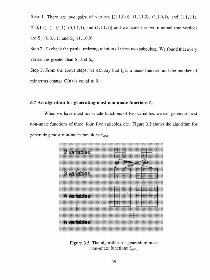
3.7 An algorithm for generating most non-unate functions fu

When we have most non-unate functions of two variables, we can generate most

non-unate functions of three, four, five variables, etc. Figure 3.5 shows the algorithm for

generating most non-unate functions f

3ov-raate f_______s___

4 variable9

n varables

Figure 3.5. The agorithm for generating mostnon-unate functions f

59

THEOREM 3.13. For n variables, there are only two most non-unate functions (fe)

and denoted as f (n) and fodg(n). Their relationship is:

QV Z2 ( ) / d[3.19]

THEOREM 3.14. Given fev (n) and fod(n), fev(n+l) and fod(n+l) can be generated

as follows.

f0 re1 2(n+1) = X +iif 2 (n) +x,.ifOdd(n) [3.20]

f e1eV f

(n+1) = f, n) +X .fl f dd (n) [3.21]

3.8 Applications

Fuzzy unate functions can be applied to switching theory, logic design, computer

design, pattern classification, pattern recognition, and pattern understanding. In this

chapter, I discuss their three applications -- function representation, data compression, and

error detection and correction.


Fuzzy unate functions can be used as a tool to represent any logic function f.

If C(n) = i, then

f = f E (ml, --. 2

60

where fu is a unate function, G indicates the exclusive or operation and i, i 2,..., mx are

interms which should be changed from fu in order to obtain f.

Example 3.9. If we want to convert f(x1 ,x2,x 3) = X(1,2,4,7) into a unate function

f(xX 2,x3), then C(f(x1,x 2 ,x3))=l and it can be represented as f(xI,x2,x 3) =

X(1,2,3,7)GX(m 3,m4).


A unate function can be represented [w,,w2,...,w.;C] which has a simpler

representation compare with a general logic function.

For function f with C(n)=i, then function f can be represented by

f=fu {mi [3.24]


corresponding Karnaugh map, we can transmit only fu and the minterms m;. Therefore,



Fuzzy unate functions also can be applied to error detection. For example, if we

know that a most non-unate function (f ) is transmitted and errors occurred, than at the

receiving end,

61

where ' indicates the function received.

We know that there are only two most non-unate functions for n variables.

Therefore, if we transmit a most non-unate function of n variables, then all the errors can

be detected and corrected.

Example 3.10. fM (x,x 2 ,x3) = (0,3,5,6;C=2) is transmitted, f(x1 ,x 2,x 3) = X(0,1,3,5;C=0)

is received. C(f (x,x 2 ,x 3))=2 is not equal to C(f(x,x 2,x3))=O. So the numbers of

minterms 1 and 5 of f are erroneous and they can be corrected.

3.9 Conclusion

Fuzzy unate functions are introduced and investigated by using the concept of

fuzzy logic. We know that there are two most non-unate functions and they are same as

the most inseparable functions of threshold functions, they are all odd function and even

function. The algorithms for determining C(n) and Cm(n), generating most non-unate

functions f are presented and illustrated with examples. About applications, fuzzy unate

functions are also applied to function representation, data compression, and error detection

and correction. The results may be have useful applications in logic design, pattern


62

Chapter Four

Flash Analog to Digital Converter

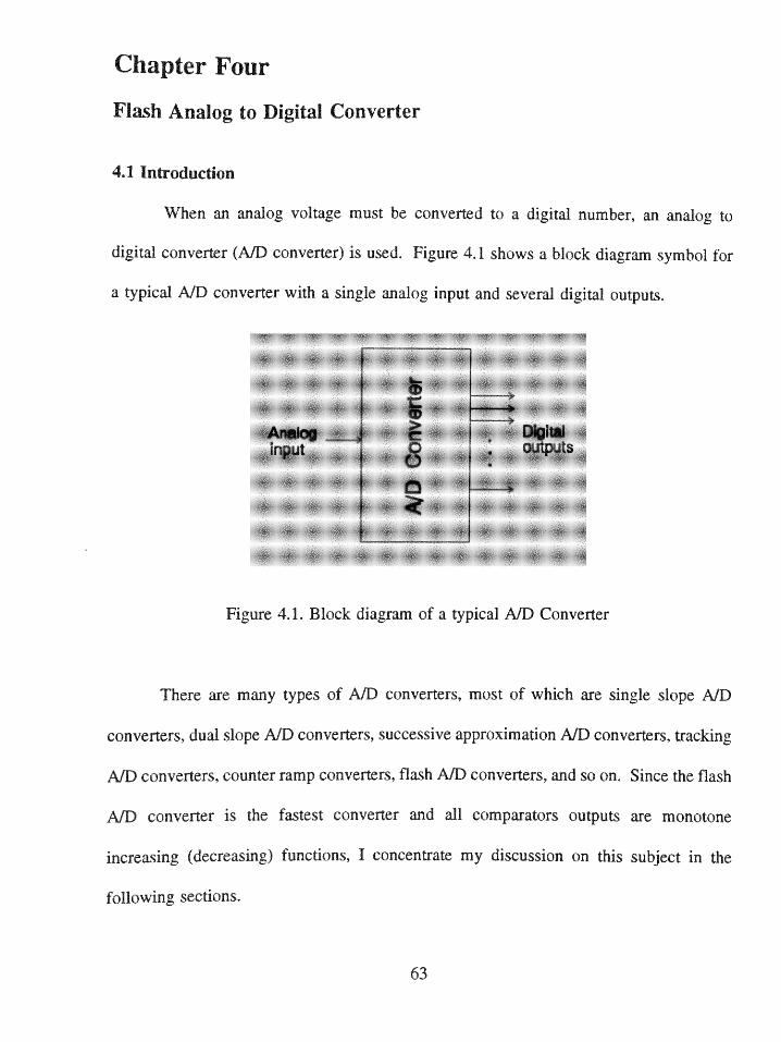
4.1 Introduction

When an analog voltage must be converted to a digital number, an analog to

digital converter (AID converter) is used. Figure 4.1 shows a block diagram symbol for

a typical A/D converter with a single analog input and several digital outputs.

Figure 4.1. Block diagra of a typical AID Converter

There are many types of A/D converters, most of which are single slope A/D

converters, dual slope A/D converters, successive approximation A/D converters, tracking

A/D converters, counter ramnp converters, flash A/D converters, and so on. Since the flash

A/D converter is the fastest converter and all comparators outputs are monotone

increasing (decreasing) functions, I concentrate my discussion on this subject in the

following sections.

63

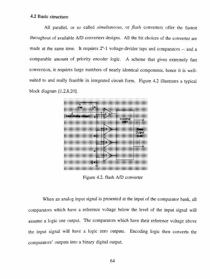
4.2 Basic structure

All parallel, or so called simultaneous, or flash converters offer the fastest

throughout of available AID converters designs. All the bit choices of the converter are

made at the same time. It requires 2- 1 voltage-divider taps and comparators -- and a

comparable amount of priority encoder logic. A scheme that gives extremely fast

conversion, it requires large numbers of nearly identical components, hence it is well-

suited to and really feasible in integrated circuit form. Figure 4.2 illustrates a typical

block diagram [1,2,8,20].

Figure 4.2. flash A/D converter

When an anlog input signal is presented at the input of the comparator bank, all

comparators which have a reference voltage below the level of the input signal will

assume a logic one output. The comparators which have their reference voltage above

the input signal will have a logic zero outputs. Encoding logic then converts the

comparators' outputs into a binary digital output.

64

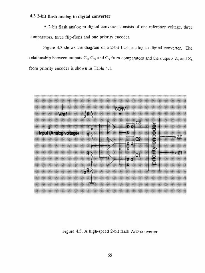
4.3 2-bit flash analog to digital converter

A 2-bit flash analog to digital converter consists of one reference voltage, three

comparators, three flip-flops and one priority encoder.

Figure 4.3 shows the diagram of a 2-bit flash analog to digital converter. The

relationship between outputs C1, C2, and C3 from comparators and the outputs Z, and Z2

from priority encoder is shown in Table 4.1.

CONV

Input~~~ ~~ (Aa1 v3ae)c

C2D Q,9-11z C 0-

Figure 4.3. A high-speed 2-bit flash A/D converter

65

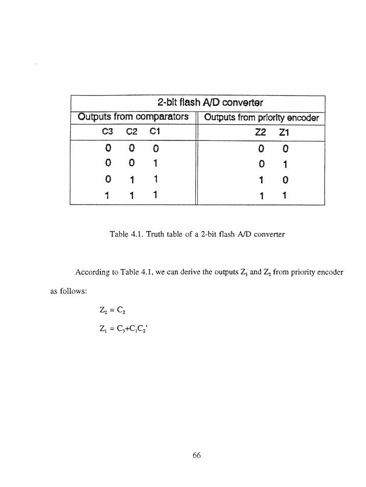
2-bit flash A/D converter

utputs from cormparators Outputs from priority encoderC3 C2 Cl Z2 Z1

0 00 0 00 01 0 10 1 1 1 0

1 1 1 1 1

Table 4.1. Truth table of a 2-bit flash A/D converter

According to Table 4.1, we can derive the outputs Z1 and Z2 from priority encoder

as follows:

Z2 = C2

ZI = C3+ClC2'

66

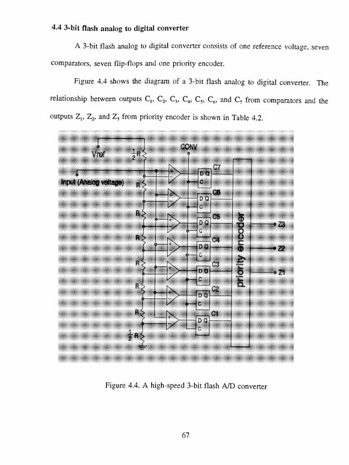
4.4 3-bit flash analog to digital converter

A 3-bit flash analog to digital converter consists of one reference voltage, seven

comparators, seven flip-flops and one priority encoder.


relationship between outputs C1, C2, C, C4 , C5, C6 , and C7 from comparators and the

outputs Z1, Z2 , and Z3 from priority encoder is shown in Table 4.2.

CONVVref }

Figre ,4 A hihee 3-i fls /cneepu6 () D

--

__ M

C '

R f


67

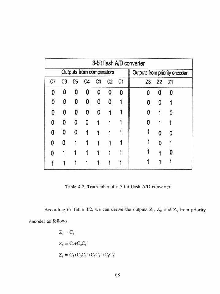
3-bft flash AD converterOutputs from comparators Outputs from priority encoder

C7 C6 C5 C4 C3 C2 C1 Z3 Z2 Z1

00 00 0 00 00 00000001 00 1

0 00 0 011 01 0

00 0 01 11 01 10 0 011 11 10 0

0 01 11 11 1 01

01 1111 11 1 110

Table 4.2. Truth table of a 3-bit flash AID converter

According to Table 4.2, we can derive the outputs Z1, Z2, and Z3 fromn priority

encoder as follows:

Z3= C+c64

Zi = C7+C3C 6'+C3 C4 '+CC 2'

68

4.5 4-bit flash Analog to digital converter

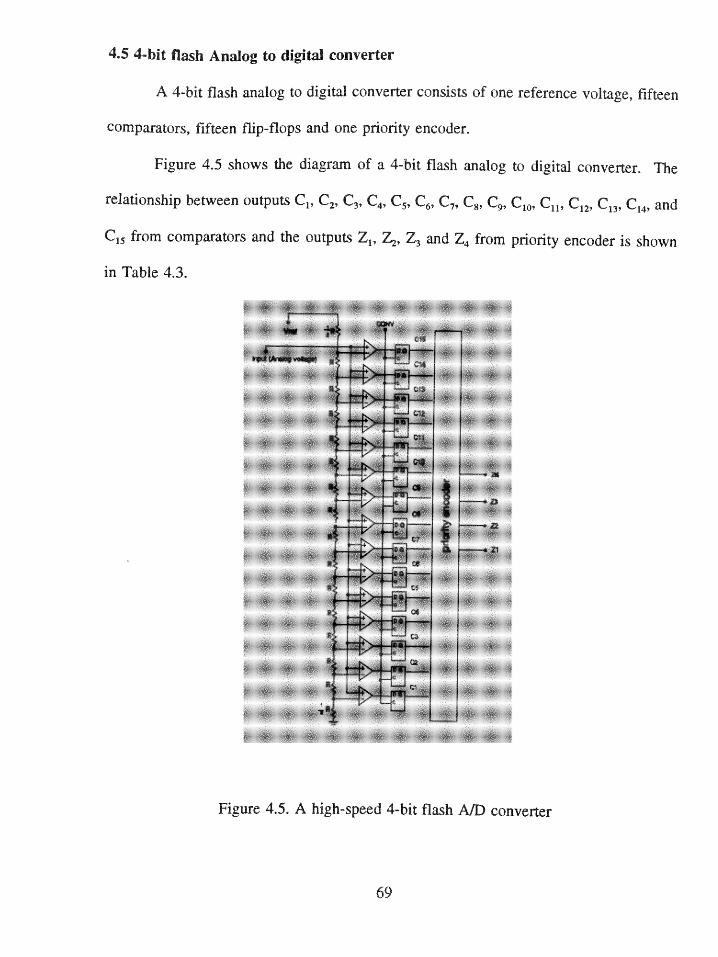
A 4-bit flash analog to digital converter consists of one reference voltage, fifteen

comparators, fifteen flip-flops and one priority encoder.


relationship between outputs C1, C2, C3, C4, C, 6 C7 C, C, CIO, 11, 12, 13 , C14, and

C15 from comparators and the outputs Z1 , Z 2, Z3 and Z4 from priority encoder is shown

in Table 4.3.


69

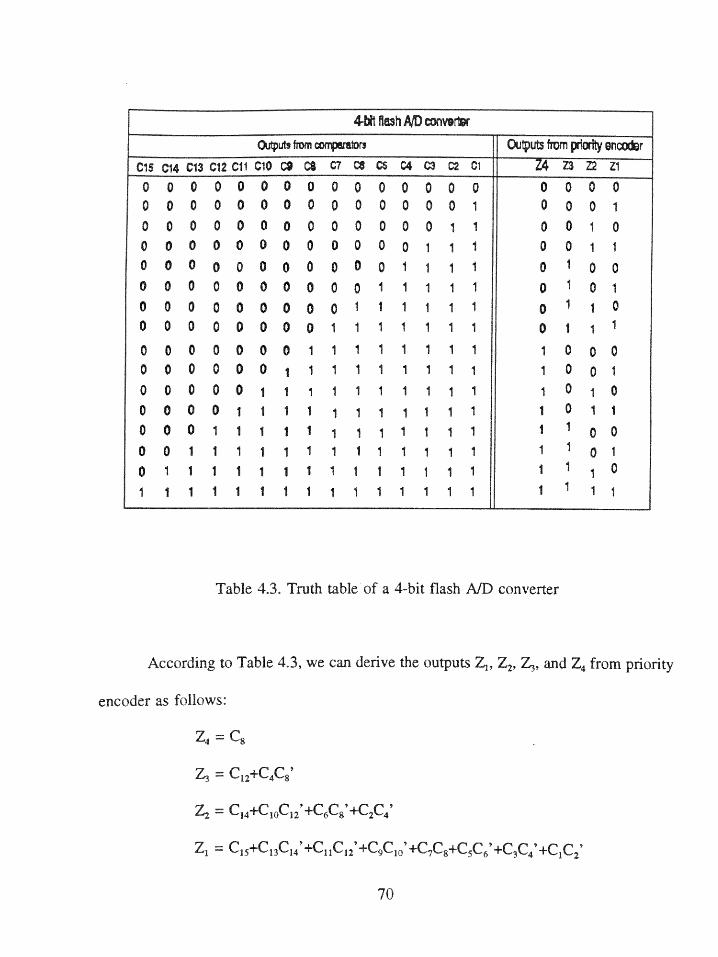
convertorA-M flash AID Outputs fmm ,., Outputs from p n

15 1 f C12 G19 C10 C9 CS C7 CS C4 6 C1

1 1

1 1 1

1 1 1 1

1 1 1 1 B 1

1 1 1 1 1 1 1

1 1 1 1 1 1 1 t

1 1 1 1 1 1 1 t 1 1

1 1 1 1 1 1 1 1 1

1 1 1 1 1 1 1 1 1 1 1

0 i t 1 1 1 1 1 1 1 1 1 1

t t t t 1 1 1 1 t 1 1 t 1

1 t t t t 1 1 1 1 1 1 1 t 1

t t t 1 1 1 t 1 1 1 1 1 1 1 1

1 t t t t t t 1 1 t 1 1 1 1 t 1 1

1 1 t t t t t t 1 1 1 1 1 1 1 t 1 1 1

Table 4.3. Truth table of 4-bit flash A/D converter

According t ale 4.3, we can derive the outputs 21 , and 4 fro priority

encoder ".31lows:

Z4 C8

9

1 l0 1 -f

T15 13 1 11 12 0 7 5 6+ 3 1 2

70

4.6 Conclusion

According to the derivations of 2-bit, 3-bit, and 4-bit flash A/D converters, we can

generalize the requirements of a n-bit A/D flash converter and the outputs' Boolean

functions from priority encoder.

(1) the requirements of a n-bit A/D flash converter are:

the number of reference voltage: 1

the number of comparators: 2"-1

the number of flip-flops: 2"-1

the number of priority encoder: 1

(2) the outputs' Boolean functions from priority encoder are:

[4.2]Z- 3*2n/4 + C1 2n/4 2 * 2 n/ 4

Zn-2 1= ,*2n + Cs *2n sC6*2n/8 3*2n/8 C4*2n/8 +C1*2n/8C * n/a

LI Ct +C[4.4]

Zn_3 = *2/'/16 13*2/16 C14*2 /16 11 *2n/16 C12*2"/16 9*2n/16 C*2n/i6

C7*2/16 C2/16 + C5*2/16 C6 *2/16 + C3*2/16 C *2n/1 + C1*2n/16 C2*2n/16

71

Chapter Five

Minimum Universal Synthesis of Logic Functions by Using MonotoneFlash Analog to Digital Converters

5.1 Introduction

In chapter 2, I mentioned that all the outputs from comparators of a n bit flash

analog to digital converter are a set of monotone increasing (decreasing) functions. Also,

through the discussion of chapter 4, it is known possible to synthesize these n binary

outputs from priority encoder by using the combination of outputs from 2"- 1 comparators

of a n-bit flash analog to digital converter. I concentrated the discussion only on

synthesizing these outputs from priority encoder. So I want to extend the discussion more

deeply about the synthesizing rules to any given function by using monotone flash analog

to digital converters in this chapter.

5.2 Rule of choosing minterms or maxterms to synthesize a given function

If a logic function is given, there must be a certain number of minterms and

maxterms. The following Lemmas will decide how to choose either minterms or

maxterms to synthesize a logic function.

LEMMA 5.1. For any given function of n variables, the absolute distance between the

number of segment of logic one and the number of segment of logic zero

should be equal to or smaller than one.

#of segment of 1 -# of segmentof 0 .[5.1]

72

IF # of segment of 1 > # of segment of 0, THEN

Using logic zero (maxterm) to synthesize the function.

IF # of segment of 0 > # of segment of 1, THEN

Using logic one (minterm) to synthesize the function.

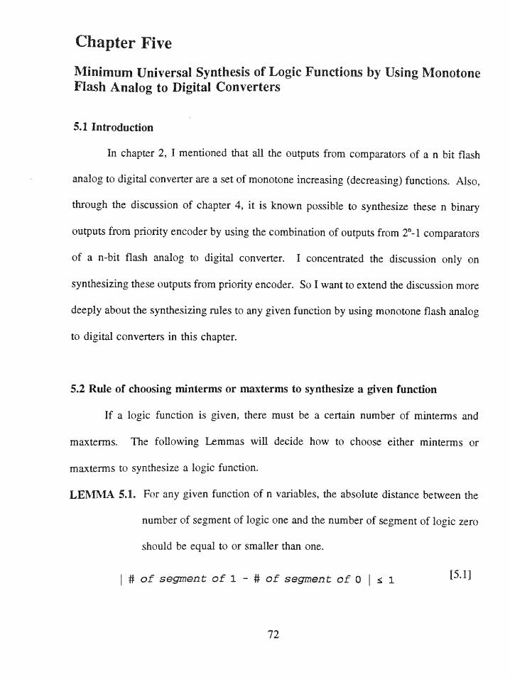
Thus, Lemma 5.1 can be transferred into Figure 5.1.

#o" segment of (mterm s)

yes

usLn aoi eo (atr using Voic one mr

Figure 5.1. The first rule for choosing minte s or maxterms

to synthesize a given function

73

Example 5.1. For a given three-variable function f(x1 ,x2 ,x3)=(1,2,6), the # of segment of

I which is equal to two is less than the # of segment of 0 which is equal to three. As

mentioned above, it is better to use logic one (minterm) to synthesize this function.

LEMMA 5.2. For any given function of n variables,

IF both the first and the last bits are logic zeros, THEN

# of segment of 0 will be greater than # of segment of 1, and THEN

Using logic one (minterm) to synthesize the function.


IF both the first and the last bits are logic ones, THEN

# of segment of 1 will be greater than # of segment of 0, and THEN

Using logic zero (maxterm) to synthesize the function.


IF the first bit is a logic one and the last bit is a logic zero , or if the first

bit is a logic zero and the last bit is a logic one, THEN

# of segment of 1 will be equal to # of segment of 0, and THEN

Using either logic one (minterm) or logic zero (maxterm) to synthesize the

function.

74

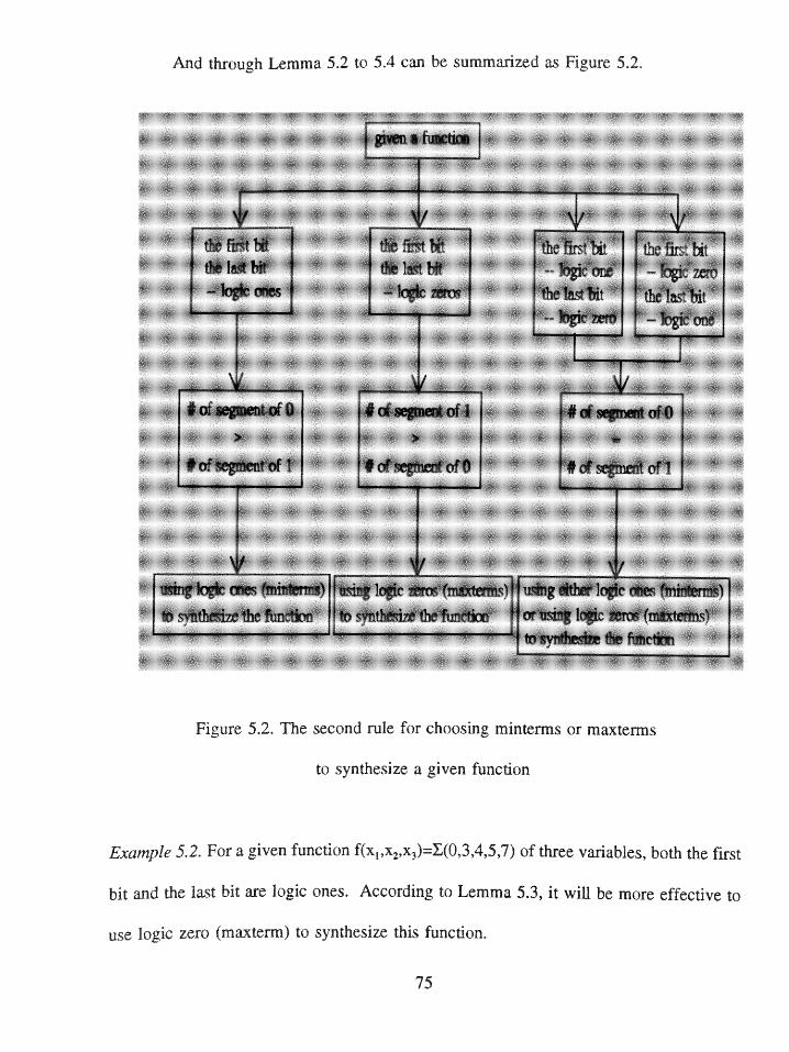
And through Lemma 5.2 to 5.4 can be summarized as Fgure 5.2.

Figre 5h2 The so nd ue. t ongin t e s o m te s t

to synthesize a given function

Example 5.2. For a given function f(x1,x2,x3)=X(O,3,4,5,7) of three variables, both the first

bit and the last bit are logic ones. According to Lemma 5.3, it will be more effective to

use logic zero (maxterm) to synthesize this function.

75

5.3 Synthesis of a logic function by using monotone flash analog to digital converters

In chapter 2, I mentioned that all the outputs from comparators of a n-bit flash

analog to digital converter are a set of monotone increasing (decreasing) functions. A

control line (CL) can be added to a flash analog to digital converter in order to converter

it as a monotone increasing flash A/D converter or a monotone decreasing flash A/D

converter. Figure 5.3 shows the diagram of a monotone flash A/D converter.

V e

Inu

Figure 5.3. monotone flash A/D converer

When CL is set to 0, the converter will become a monotone increasing flash A/D

converter.

When CL is set to 1, the converter will become a monotone decreasing flash A/D

converter.

76

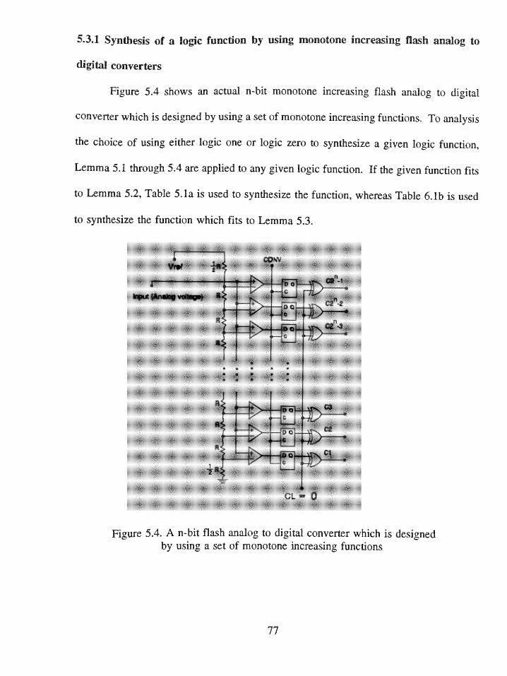
5.3.1 Synthesis of a logic function by using monotone increasing flash analog to

digital converters

Figure 5.4 shows an actual n-bit monotone increasing flash analog to digital

converter which is designed by using a set of monotone increasing functions. To analysis

the choice of using either logic one or logic zero to synthesize a given logic function,

Lemma 5.1 through 5.4 are applied to any given logic function, If the given function fits

to Lemma 5.2, Table 5.1a is used to synthesize the function, whereas Table 6.1b is used

to synthesize the function which fits to Lemma 5.3.

bypu using lawa se fmntn ncesn ucint n7I vo j

'sc

n3

Figure 5.4. A n- bit flash analog to digital converter wich is designedby using a set of monotone increasing functions

77

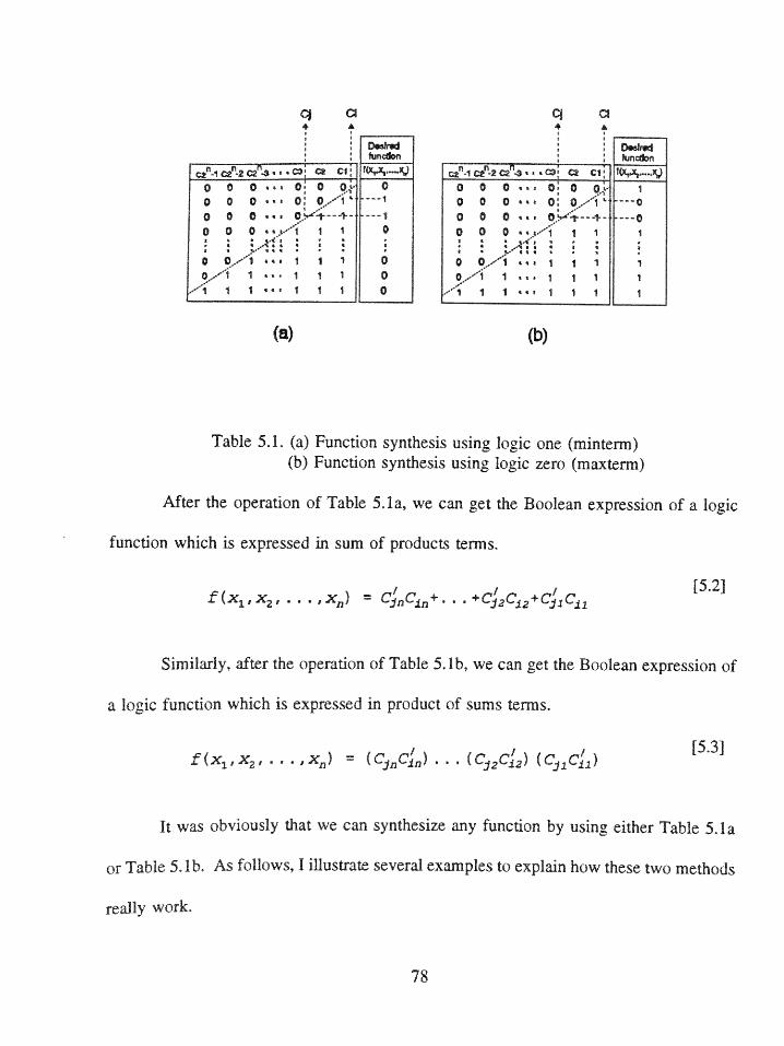
q a : a

f uncdon R n po

o . 0 0 0~ 0 .4 e 0o o o o: o .0 L ~1 0 0 0 o 1L -0

o 0 0 ' 0 + -1 0 0 0C2 0'-+- -0o 0 0 1 1 1 o 0 0 '

o * 1 1 0 o 0,is 101S i1 1 1 0 1 ... 1 1 1

1 1 i 1 1 1 0- 1 1 aP 1 1 1

Table 5.1. (a) Function synthesis using logic one (minterm)(b) Function synthesis using logic zero (maxterm)

After the operation of Table 5. a, we can get the Boolean expression of a logic

function which is expressed in sum of products terms.

ff( x11,x 2, . -- . = CynCin+ . [5 +,21 +c',s

Similarly, after the operation of Table 5.1b, we can get the Boolean expression of

a logic function which is expressed in product of sums terms.

f xx, 2 -- ' n)= ( CanCs') . . . (fC12 C12 ) ( Cy1CI,)[53

It was obviously that we can synthesize any function by using either Table 5.la

or Table 5.1 b. As follows, I illustrate several examples to explain how these two methods

really work.

78

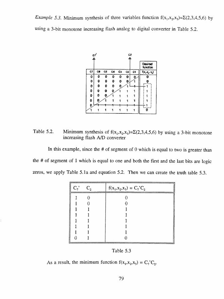
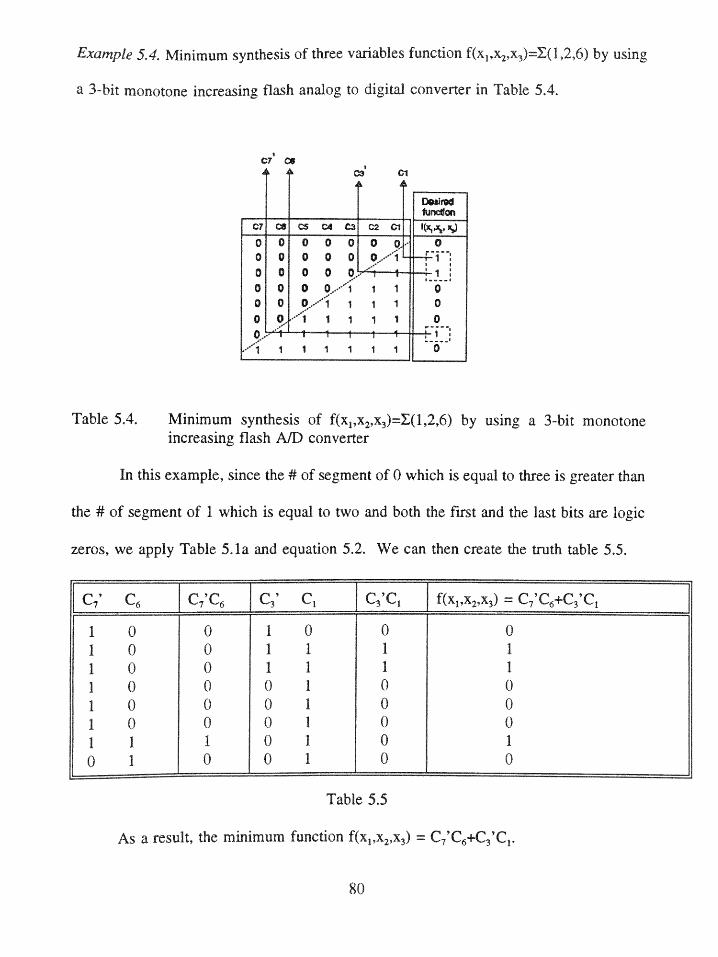
Example 5.3. Minimum synthesis of three variables function f(x1 ,x 2,x3)= (2,3,4,5,6) by

using a 3-bit monotone increasing flash analog to digital converter in Table 5.2.

07' 02

_uncdon

C? CO CS 04 C3 02 c f ,

o 0 0 0 0 0o 0.0 0 0 0 O . -i

o o o 4 1 1 1"1 1 1 1

o ..--'1 1 1 1 1 = 1

'1 1 1 1 1 1 1 0

Table 5.2. Minimum synthesis of f(x1,x 2 ,x 3)=(2,3,4,5,6) by using a 3-bit monotoneincreasing flash A/D converter

In this example, since the # of segment of 0 which is equal to two is greater than

the # of segment of 1 which is equal to one and both the first and the last bits are logic

zeros, we apply Table 5.la and equation 5.2. Then we can create the truth table 5.3.

C7' C2 J fXIIX2?X3) = CC 2

1 0 01 0 01 1 11 1 11 1 11 1 11 1 10 1 0

Table 5.3

As a result, the minimum function f(x1 ,x 2 ,x 3) =C7'C2

79

Example 5.4. Minimum synthesis of three variables function f(x1 ,x 2 ,x 3)=(1,2,6) by using

a 3-bit monotone increasing flash analog to digital converter in Table 5.4.

C7 C7

CS 01

DsirPd

S 0 0 0 0 O 00 0 0 00 0710 0 00 0 10 0 0 Q.."1 1 1 0

0 ,l 1 1 1 00 0 1 1 1 1 0

®

e

1 1 1 1 1 1 1 0

Table 5.4. Minimum synthesis of f(xl,x2 ,x 3)=(1,2,6) by using a 3-bit monotoneincreasing flash A/D converter

In this example, since the # of segment of 0 which is equal to three is greater than

the # of segment of 1 which is equal to two and both the first and the last bits are logic

zeros, we apply Table 5.la and equation 5.2. We can then create the truth table 5.5.

C C CC6 JC 36 C3 C3'C1 jf(x 1,x2,x3) = C 6'C6+C3' C1

1 0 0 1 0 0 01 0 0 1 1 1 11 0 0 1 1 1 11 0 0 0 1 0 01 0 0 0 1 0 01 0 0 0 1 0 01 1 1 0 1 0 10 1 0 0 1 0 0

Table 5.5

As a result, the minimum function f(x1 ,x 2 ,x 3 ) = ,'C+C3'C1.

80

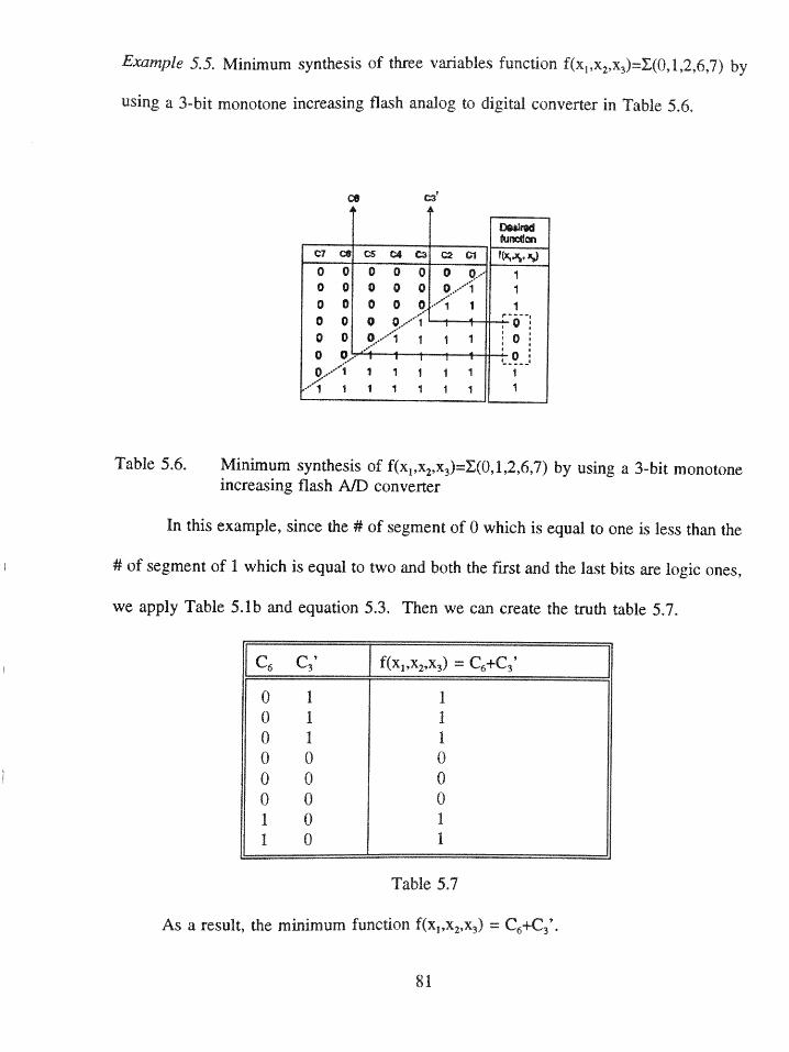
Example 5.5. Minimum synthesis of three variables function f(x1,x 2,x 3)=(0,1,2,6,7) by


C7 CS cs C4 i ff ,o 0 0 0 0 0 - 1o 0 0 0 0 0o.o 0 0 0 O --i 1o 0 0 0,'1o 0 o. 1 i 1o oi0,--'1 1 1 1 1 1 1

<-'"®1 1 1 1 1 1 1 1

Table 5.6. Minimum synthesis of f(x1,x 2,x3)=X(0,1,2,6,7) by using a 3-bit monotoneincreasing flash A/D converter

In this example, since the # of segment of 0 which is equal to one is less than the

# of segment of 1 which is equal to two and both the first and the last bits are logic ones,

we apply Table 5.1b and equation 5.3. Then we can create the truth table 5.7.

C6 C3 f(x1,x2,x3) =CC

0 1 10 1 10 1 10 0 00 0 00 0 01 0 11 01

Table 5.7

As a result, the minimum function f(xl,x2,x3) = 3'.

81

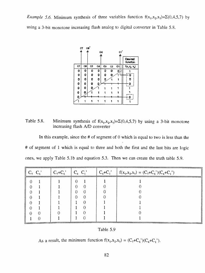
Example 5.6. Minimum synthesis of three variables func mon f(x1 x2,x 3)=X(0,4,5,7) by


Ay C404 ci'

_____funcdon

07 06 CS C4 Ca 02 01 (

S0 0 0 0.. 100 o 0 -. *000 0'</ 1 1 1 1S0,."1 1 1 1 1 1

/1 1 1 1 1 1 1

Table 5.8. Minimum synthesis of f(x1,x 2 ,x 3)=(0,4,5,7) by using a 3-bit monotoneincreasing flash A/D converter

In this example, since the # of segment of 0 which is equal to two is less than the

# of segment of 1 which is equal to three and both the first and the last bits are logic

ones, we apply Table 5.1b and equation 5.3. Then we can create the truth table 5.9.

C7 C+C C4 C' C4 f(x 1 ,x2,x3 ) 7(C+C6')(C+C 1})

0 1 1 0 1 1 10 1 1 0 00 1 1 0 0 0 001 1 0 0 0 00 1 1 1 0 1 10 1 1 10 1 10 0 0 10 1 01 0 1 1 0 1 1

Table 5.9

a result, the minimum function f(xl,x2 ,x 3) = (C6+C')(C4 +C1').

82

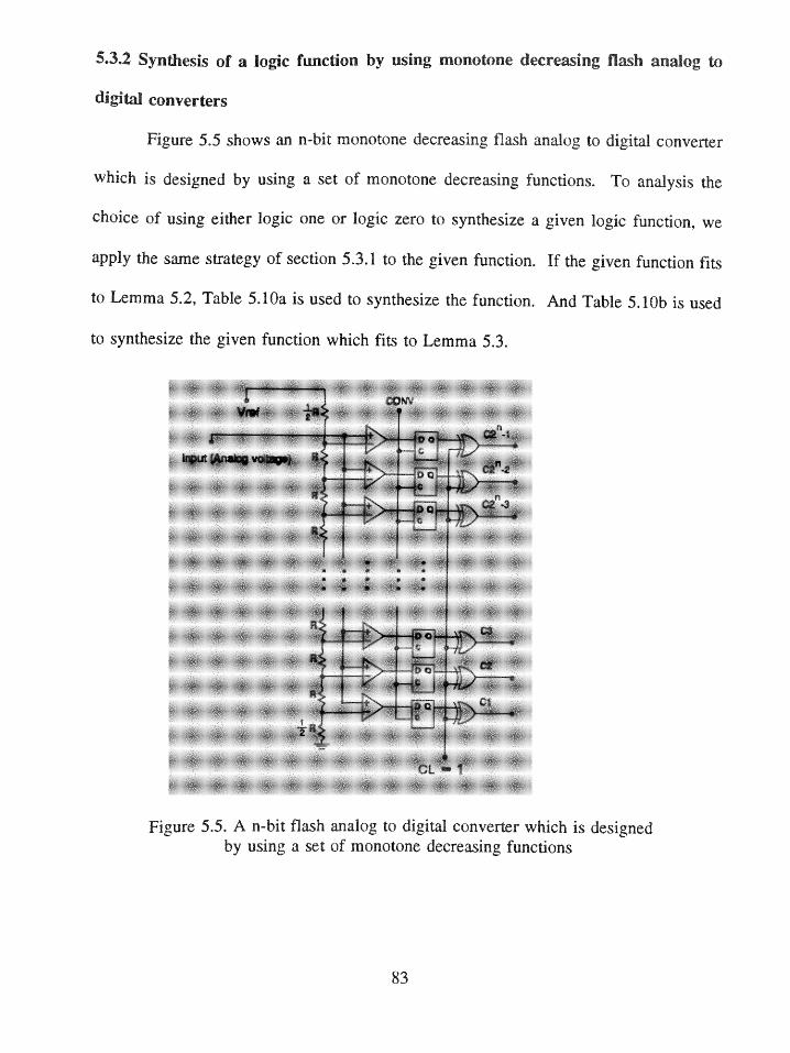
5.3.2 Synthesis of a logic function by using monotone decreasing flash analog to

digital converters

Figure 5.5 shows an n-bit monotone decreasing flash analog to digital converter

which is designed by using a set of monotone decreasing functions. To analysis the

choice of using either logic one or logic zero to synthesize a given logic function, we

apply the same strategy of section 5.3.1 to the given function. If the given function fits

to Lemma 5.2, Table 5.10a is used to synthesize the function. And Table 5.10b is used

to synthesize the given function which fits to Lemma 5.3.

Figu55 $n-bi fltash anlgt ii ov hc sdsgeVrof

7

r6a

by using a set of monotone decreasing functions

83

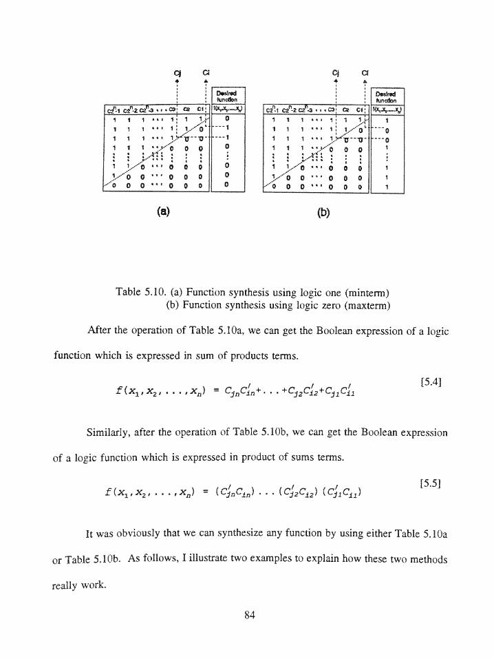
C11 ci1- __ _ 2 C24 11 C : l 1C1 A ...

1 1 1 a s f a 1. _ 1 1 '.a xo

1 1 1 **v' 0 0 0 1 1 1 *y0 0 0 1

1 1 0w**0 0 0 0 1 1 o03 o 0 *- 0 0 0 1/0 0 ''0 0 0 1

t 0 O 0 0 0 0 0 0 O 0 0 1

(a) (b)

Table 5.10. (a) Function synthesis using logic one (minterm)(b) Function synthesis using logic zero (maxterm)

After the operation of Table 5.10a, we can get the Boolean expression of a logic

function which is expressed in sum of products terms.

Similarly, after the operation of Table 5.10b, we can get the Boolean expression

of a logic function which is expressed in product of sums terms.

) [5.5]S(x 1 x, - -.. n = ( C9'C 1.) . .. ( C)~2 C12 ) ( C)' 1C11)

It was obviously that we can synthesize any function by using either Table 5.1 a

or Table 5.1 b. As follows, I illustrate two examples to explain how these two methods

really work.

84

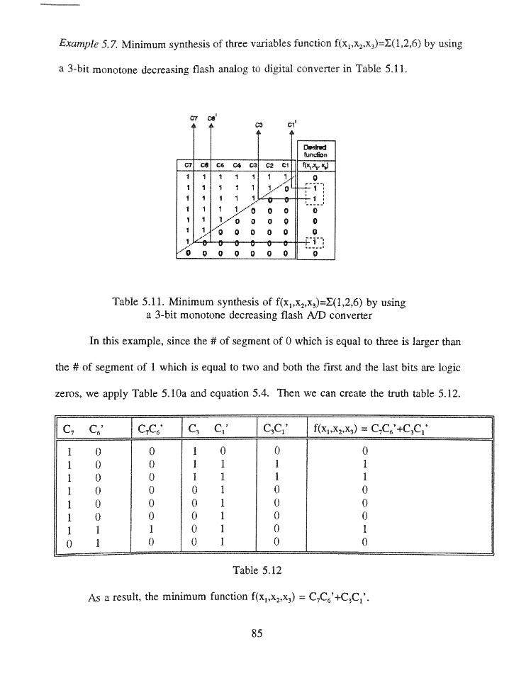
Example 5,7. Minimum synthesis of three variables function f(x1 x2 x3)= (1,2,6) by using

a 3-bit monotone decreasing flash analog to digital converter in Table 5.11.

07 Ce03 C1

07 C4 06 04 03 02 C1 ;

1 1 1 1 1 1 . 0 -9

C)01 1 1

1 1

1 1,,

f 1 i 1 1 1, f.

1 1 1 0 0 0 0

1 !-"o 0 0 0 0

Table 5.11. Minimum synthesis of f(x1,x 2 ,x3)=(1,2,6) by usinga 3-bit monotone decreasing flash A/D converter

In this example, since the # of segment of 0 which is equal to three is larger than

the # of segment of 1 which is equal to two and both the first and the last bits are logic

zeros, we apply Table 5.10a and equation 5.4. Then we can create the truth table 5.12.

C7 C' C7C6' C C1 I f(xx x3) = CC '+C

1 0 0 1 0 0 01 0 0 1 1 1 11 0 0 1 1 1 11 0 0 0 1 0 01 0 0 0 1 0 01 0 0 0 1 0 01 1 1 0 1 0 10 1 0 0 1 0 0

Table 5.12

As a result, the minimum function f(x1,x 2 ,x 3) = C7C'+C3C1'.

85

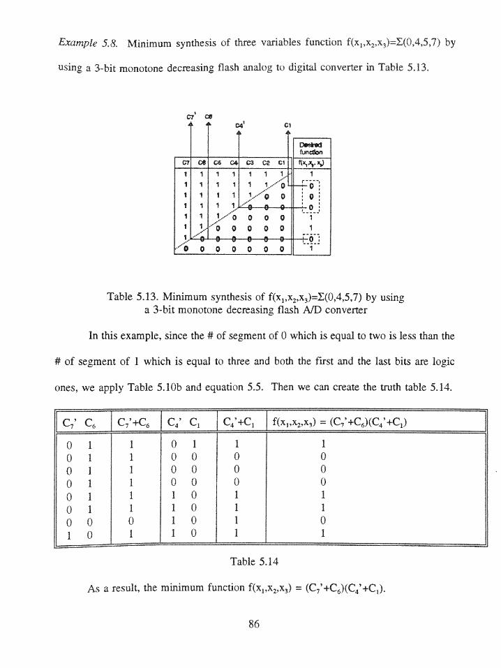
Example 5.8. Minimum synthesis of three variables function f(x x x ()=(0 47) by

using a 3-bit monotone decreasing flash analog to digital converer in Table 5.13.

& asC4 C1

C? CO C6 C4 C3 CU Cl

1 1 1 1 1 1 1o

1 1'0 0 0 0 0 1

Table 5.13. Minimum synthesis of f(x1,x 2,x3)=X(0,4,5,7) by usinga 3-bit monotone decreasing flash A/D converter

In this example, since the # of segment of 0 which is equal to two is less than the

# of segmnent of 1 which is equal to three and both the first and the last bits are logic

ones, we apply Table 5.10b and equation 5.5. Then we can create the truth table 5.14.Cabl C6 13 [iiu Cynthesi j_ 4 Cf 4 C f(x,x 2 ,x3) = (,4,5,7)(Cyusing

0 1 1 0 1 1 10 1 1 0 0 0 00 1 1 0 0 0 00 1 1 0 0 0 00 1 1 1 0 1 10 1 1 1 0 1 10 0 0 1 0 1 010 1 10 1 1

Table 5.14

As a result, the minimu function f(xx 2,x3) =

86

5.4 Conclusion

After the above illustrations, we can synthesize any given function by using either

monotone increasing flash A/D converters or monotone decreasing flash A/D converters.

The rules of how to synthesize a given function are also presented and illustrated by

examples. It can be applied usefully to logic design, computer design, and other related

areas.

87

Chapter Six

Fuzzy Classification

6.1 Introduction

After the discussion of fuzzy threshold functions, fuzzy monotone functions, and

fuzzy unate functions, there are many results that can be generalized and we can find

some relationships from these results. Furthermore, if a function is given, I try to classify

this function that should be belonged to which special logic function.

The grade of membership function p is normalized in the interval [0 1] and it is

set to be 1 if the function is a specific special logic function. So general speaking, when

we have many special logic functions and want to classify them, the larger grade of

membership function p, the stronger connection to the class function. Therefore, the

classification is based upon fuzzy sets theory and I restrict that there are only four fuzzy

special logic functions when I investigate the classification procedure, they are fuzzy

threshold functions, fuzzy monotone increasing functions, fuzzy monotone decreasing

functions, and fuzzy unate functions. After the discussion, readers will find that the

classification procedure can be usefully applied to any other special logic functions.

88

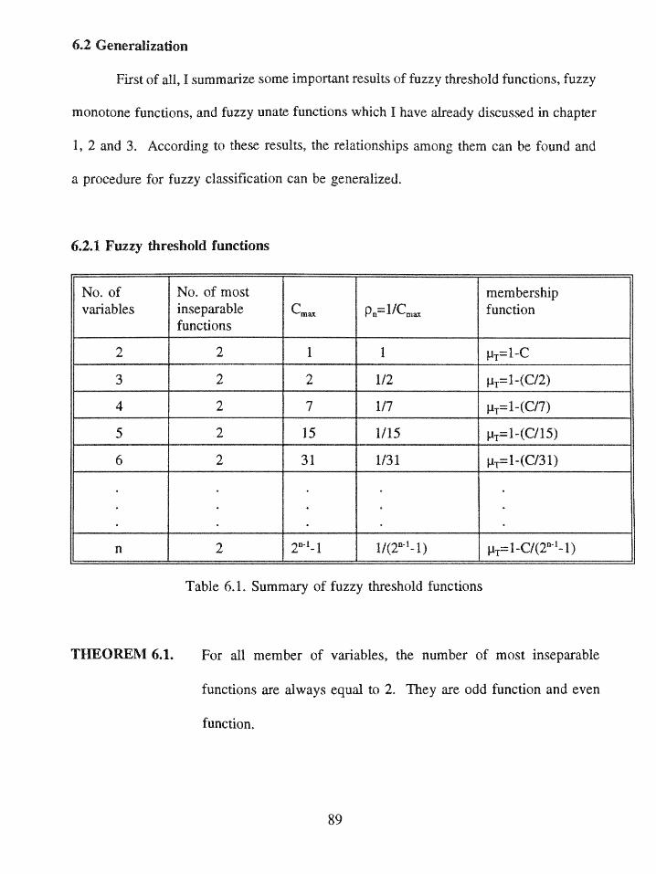
6.2 Generalization

First of all, I summarize some important results of fuzzy threshold functions, fuzzy

monotone functions, and fuzzy una functions which I have already discussed in chapter

1, 2 and 3. According to these results, the relationships among them can be found and

a procedure for fuzzy classification can be generalized.

6.2.1 Fuzzy threshold functions

No. of No. of most membershipvariables inseparable C Pn=1/Cmax function

functions

2 2 1 1 PT=1-C

3 2 2 1/2 pT=- (C/2)

4 2 7 1/7 pT=( /7)

5 2 15 1/15 pT=1-(C/15)

6 2 31 1/31 pT=1-(C/31)

n 2 2n-1- 1/(2" -1) p=1-C/(2"n-1)

Table 6.1. Summary of fuzzy threshold functions

THEOREM 6.1. For all member of variables, the number of most inseparable

functions are always equal to 2. They are odd function and even

function.

89

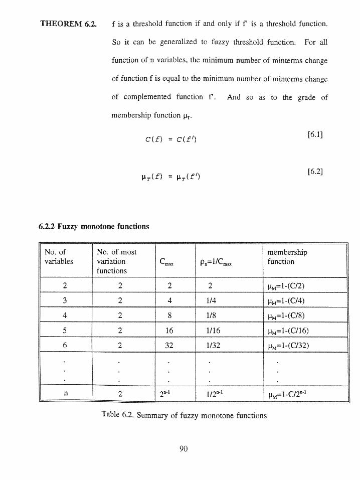
THEOREM 6.2. f is a threshold function if and only if f is a threshold function.

So it can be generalized to fuzzy threshold function. For all

function of n variables, the minimum number of minterms change

of function f is equal to the minimum number of minterms change

of complemented function f. And so as to the grade of

membership function p1 .

C(f) = C(f') [6.1]

C(f) = f [6.2]

6.2.2 Fuzzy monotone functions

No. of No. of most membershipvariables variation Cm p=l/Cma function

functions

2 2 2 2 p=1-(C/2)

3 2 4 1/4 pM=1-(C/4)

4 2 8 1/8 p=1-(C/8)

5 2 16 1/16 p =1-(/C16)

6 2 32 1/32 p=1-(C/32)

n q2 2n-I 1/2I p =

Table 6.2. Summary of fuzzy monotone functions

90

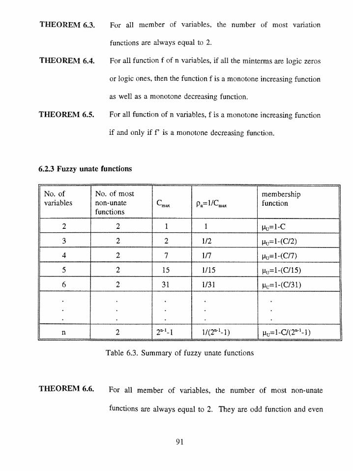
THEOREM 6.3. For all member of variables, the number of most variation

functions are always equal to 2.

THEOREM 6.4. For all function f of n variables, if all the minterms are logic zeros

or logic ones, then the function f is a monotone increasing function

as well as a monotone decreasing function.

THEOREM 6.5. For all function of n variables, f is a monotone increasing function

if and only if f' is a monotone decreasing function.

6.2.3 Fuzzy unate functions

No. of No. of most membershipvariables non-unate C. Pn=l/Cma function

functions

2 2 1 1 pU=1-C

3 2 2 1/2 pu=1-(C/2)

4 2 7 1/7p=1-(/

5 2 15 1/15 p=1-(C/1)

6 2 31 1/31 pu=1-(C/31)

n 2 2"4-1 1/(2"p-1) pu=1-C/(2"n-1)

Table 6.3. Summary of fuzzy unate functions

THEOREM 6.6. For all member of variables, the number of most non-unate

functions are always equal to 2. They are odd function and even

91

function.

THEOREM 6.7. f is a unate function if and only if f is a unate function. So for all

functions of n variables, the minimum number of minterms change

of function f is equal to the minimum number of minterms change

of complemented function f' And so as to the grade of

membership function pu.

C(f) C(f') [6.3]

From the summaries of fuzzy special logic functions, I conclude the following

theorems.

THEOREM 6.8. The number of most inseparable functions, most variation

functions, and most non-unate functions are all equal to 2. In

particular, the two most inseparable functions are as same as the

two most non-unate functions. They are all odd function and even

function.

Since that, the algorithms of fuzzy threshold functions and fuzzy unate functions

for generating these two functions are the same.

THEOREM 6.9. For any function of n variables, the maximum number of minterms

change C of fuzzy threshold functions is the same as the value of

fuzzy unate functions.

92

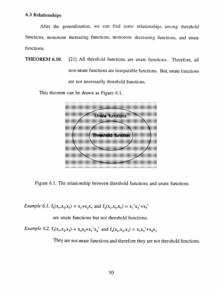
6.3 Relationships

After the generalization, we can find some relationships among threshold

functions, monotone increasing functions, monotone decreasing functions, and unate

functions.

THEOREM 6.10. [21] All threshold functions are unate functions. Therefore, all

non-unate functions are inseparable functions. But, unate functions

are not necessarily threshold functions.

This theorem can be drawn as Figure 6.1.

Figure 6.1. The relationship between threshold functions and unate functions

Example 6.1. f1(XI,X 2,X3) = X1+X 2X3 and f2 (X1,X2,X3) = X1'X2'+X3'

are unate functions but not threshold functions.

Example 6.2. f3(XI,X 2,X3) = X1X2+X,'X 2' and f4 (X1,X 2 ,X3) = X1X2 '+X2X3

They are not unate functions and therefore they are not threshold functions.

93

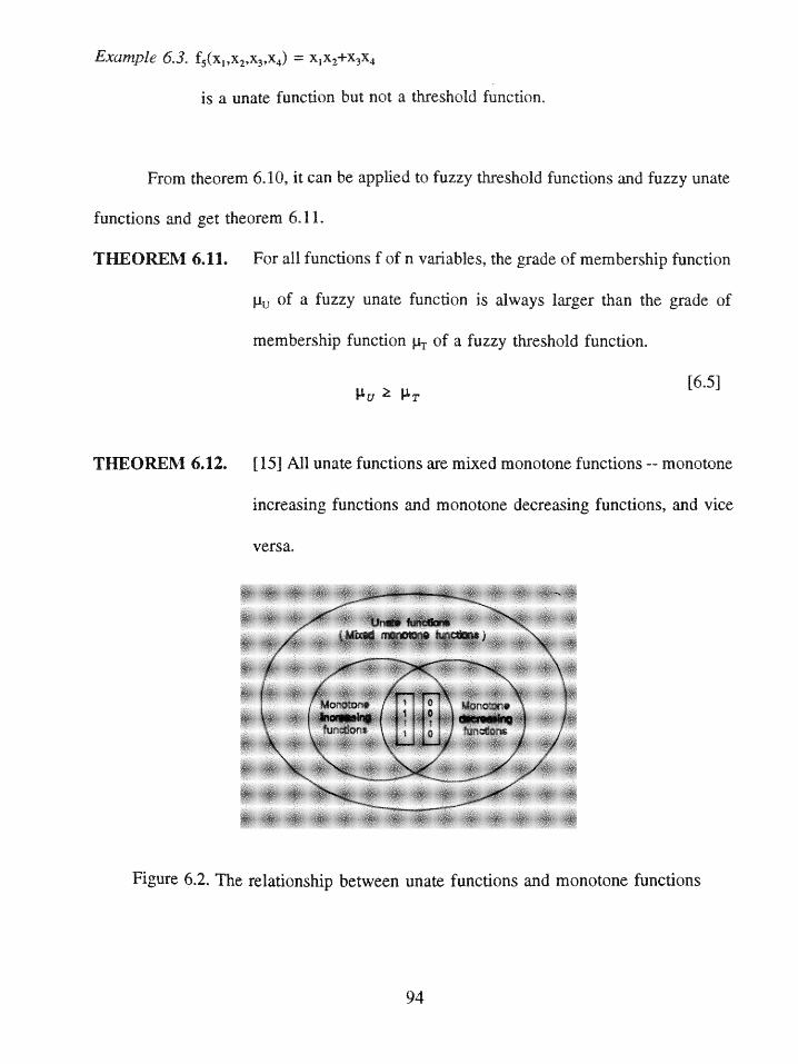
Example 6.3. f5(x),x2 ,x3,X4 = XIX2+x3X4

is a unate function but not a threshold function.

From theorem 6.10, it can be applied to fuzzy threshold functions and fuzzy unate

functions and get theorem 6.11.

THEOREM 6.11. For all functions f of n variables, the grade of membership function

p of a fuzzy unate function is always larger than the grade of

membership function pT of a fuzzy threshold function.

[6.5]

THEOREM 6.12. [15] All unate functions are mixed monotone functions -- monotone

increasing functions and monotone decreasing functions, and vice

versa.

Figure 6.2. The relationship between unate functions and monotone functions

94

Theorem 6.12 can be applied to fuzzy unate functions and fuzzy monotone

functions and we can get theorem 6.13.

THEOREM 6.13. For all functions f of n variables, the grade of membership function

pu of a fuzzy unate function is always larger than the grade of

membership function pM of a fuzzy monotone function.

p1'(f) Mz p®I6

THEOREM 6.14. For all functions f of n variables, then the minimum number of

minterms change in order to convert f to be a monotone increasing

function (fc) is equal to the minimum number of minterms

change in order to convert f' to be a monotone decreasing function

(f'MDEc

CMINC f1x, X2, . . , X))} = CMDEC ffx, X 2 , . .. ,x~ Xn [6,8]

CMEC (fX, X2, ... , Xn)) = IC ( , . . ,x) 6.9

THEOREM 6.15. For all functions f of n variables, then the grade of membership

function pMme of a fuzzy monotone increasing function f is equal

to the grade of membership function EC of a fuzzy monotone

decreasing function f.

95

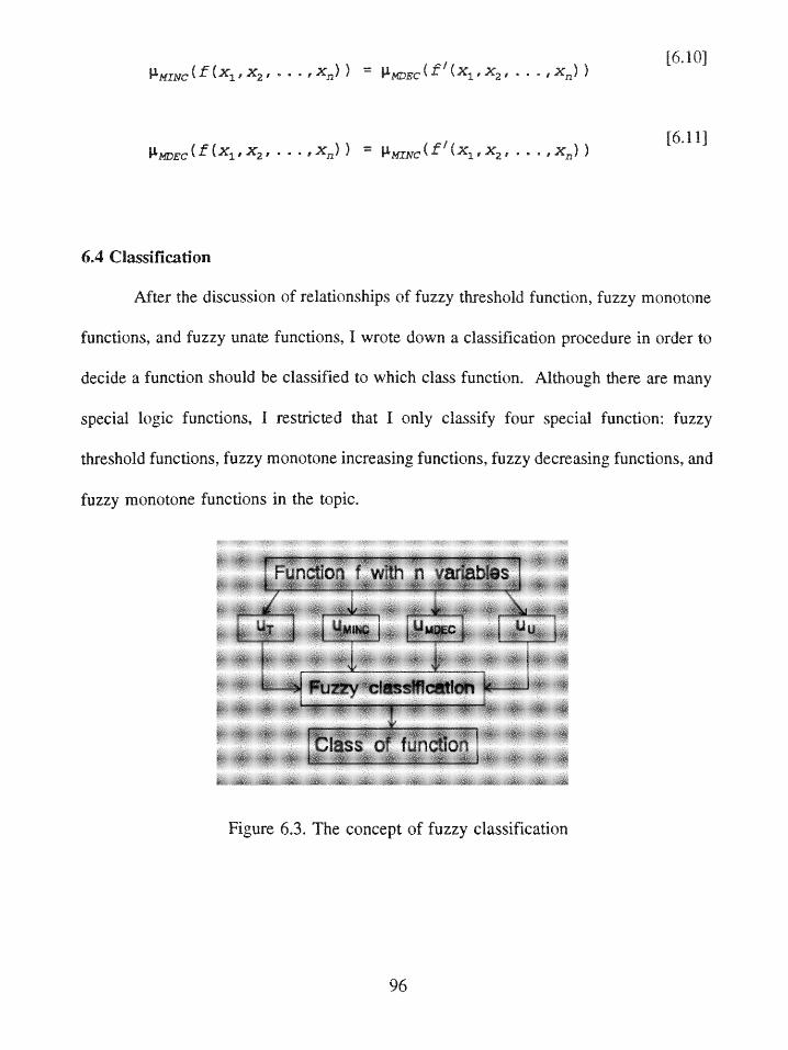
MINC 1, X 2 , ... ,x)) = %EC l(X, 2 , ... ,X) [

p~EC XX 2, .. . ,x) Xn MINC~ (X~ 2 , . [6.11]

6.4 Classification

After the discussion of relationships of fuzzy threshold function, fuzzy monotone

functions, and fuzzy unate functions, I wrote down a classification procedure in order to

decide a function should be classified to which class function. Although there are many

special logic functions, I restricted that I only classify four special function: fuzzy

threshold functions, fuzzy monotone increasing functions, fuzzy decreasing functions, and

fuzzy monotone functions in the topic.

Functon fwith n variables

Fuzz cassi l y..

Cls fin f

Figure 6.3. The concept of fuzzy classification

96

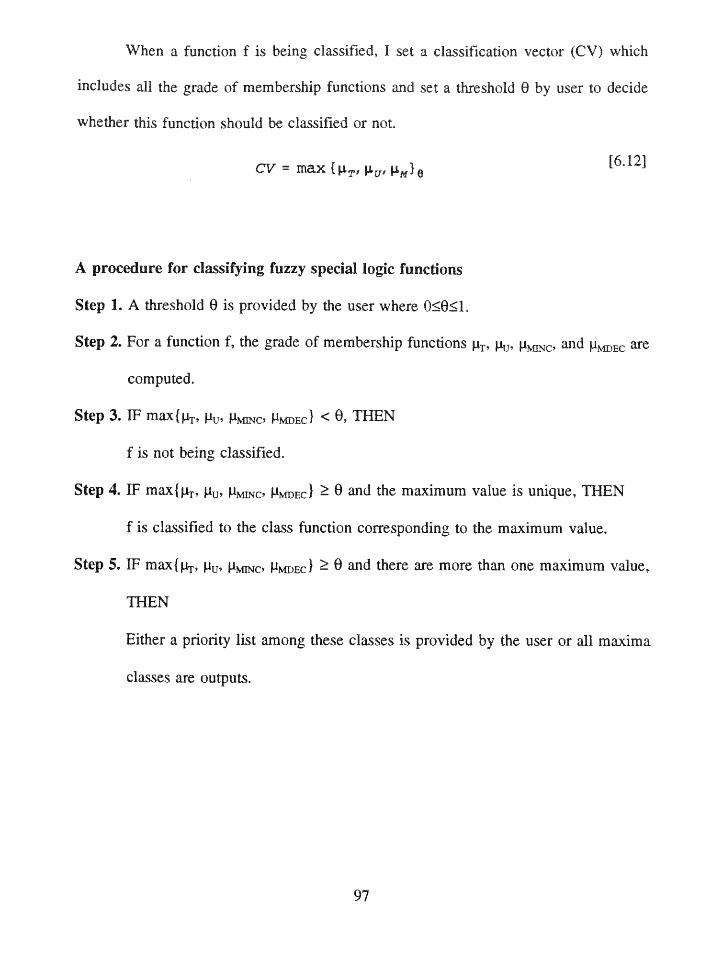
When a function f is being classified, I set a classification vector (CV) which

includes all the grade of membership functions and set a threshold 0 by user to decide

whether this function should be classified or not.

CV = max {I.pT, pa IpL}O [6.121

A procedure for classifying fuzzy special logic functions

Step 1. A threshold 0 is provided by the user where 0 0 1.

Step 2. For a function f, the grade of membership functions pT, , p and p MDEC ae

computed.

Step 3. IF max{pT, p, pM pMDEC} <0, THEN

f is not being classified.

Step 4. IF max{pT, pu, p c, PMDEC} 0 and the maximum value is unique, THEN

f is classified to the class function corresponding to the maximum value.

Step 5. IF max{IpT, p p MDEC} 0 and there are more than one maximum value,

THEN

Either a priority list among these classes is provided by the user or all maxima

classes are outputs.

97

Example 6.4. For a three-variable function f2 (x1,x2 x3) = X1+X2'x 3

Step 1. To set a threshold 0 which equals to 0.5. If maX pr, pe, CMC, pMEC} < 0.5, we

decide not to classify this function. But if max{kp, p, pMI, pMDEC} 0.5, we decide

to classify this function.

Step 2. To calculate the grade of membership functions p-, pe , p e, and pMDEC'

It is a threshold function and the grade of membership function pT is equal to 1.

It is also a unate function and the grade of membership function pc is equal to 1.

But it is neither a monotone increasing function nor monotone decreasing function.

If we want to convert f2(x1,x2,x3)=(1,3,4,5,7) into a monotone increasing function

f C(xIx 2 ,x3), then it becomes as f C(x1,x2,x3)= (3,4,5,6,7) and the number of minterms

changes C(f(x1 ,x 2,x3))=2. So pj #c=(2 /4 )=0.5. If we want to convert

f2(x1,x2, 3)=(1,3,4,5,7) into a monotone decreasing function fMEc(X1,X 2,X 3), then it

becomes as fMEc(xl,x 2 ,x 3 )=X(0,1, 2 ,3 ,4 ,5) and C(f(x1,x2,x 3))=3. So the grade of

membership function pDEc=( 3/4 )=0.7 5.

Step 3. To decide the function should be classified to which class function.

Now max{pT, pu, N JpMDEC = max{ 1,1,0.5,0.751 = 1 > 0.5. According to step

5 of the algorithm, we have the following two possible results.

(1) All the maxima classes are outputs. So this function is a fuzzy threshold

function and it also is a fuzzy unate function.

(2) According to theorem 6.11, we can say that a fuzzy threshold function is

superior to a fuzzy unate function. As a result, we classify this function as a fuzzy

threshold function.

98

6.5 Conclusion

Fuzzy threshold functions, fuzzy monotone functions, and fuzzy monotone

functions are discussed and summarized. Using fuzzy logic theory to classify a function

is discussed and a procedure for classifying fuzzy special logic functions is also presented.

Although I only discuss four fuzzy special logic functions here, this procedure is useful

to extend to all fuzzy special logic functions. And since the threshold 0 is decided by

user, the classification becomes more flexible.

99

Chapter Seven

Recommendations

(1) It is essential to apply fuzzy logic to the other special logic functions.

(2) It is necessary to investigate these four fuzzy special logic functions with don't-

care conditions.

(3) It is worthwhile to identify each group of fuzzy special logic function by its

distance (the minimum minterms change) to full membership functions.

(4) Since all the logic functions can be represented by fuzzy special logic functions,

the results of these four fuzzy special logic functions may be applied to pattern

recognition.

100

(1) C. L. Phillips and H. T. Nagle, Dii ontrol Sys alysis esin, 1990.

(2) Daniel H. Sheingold, na igital onversio Hno, 1986.

(3) E. A. Parr, The Logc esigner's uidebook, 1984.

(4) E. T. Lee, "Shape-Oriented Chromosome Classification", IEEE Tranactionson

Systems, Man and Cy etic, VolSMC-5, No.6, November, 1975, pp.629 -6 32 .

(5) E. T. Lee and L. A. Zadeh, "Note on Fuzzy Languages", Information Sciences,

Vol.1, 1969, pp.42 1-434.

(6) E. T. Lee, "Pictorial Data Compression Using Array Grammars", Proc. of the Data

Compression Conference, April 8-10, 1991, Snowbird, Utah.

(7) E. T. Lee, "Pictorial Data Compression Techniques", Proc. of the Data

Compression Conference, April 8-10, 1991, Snowbird, Utah.

(8) Eugene R. Hnatek, A User's Handbook of D/A and A/D Converters, 1976.

(9) H. T. Nagle, Jr., B. D. Carroll, and J. D. Irwin, An Introduction to Computer

_gic, 1975.

(10) James C. Bezdek, Pattern Recognition with Fuzzy Objective Function Algorithms,

1981.

(11) John D. Lenk, Logic Designer's Manual 1977.

(12) Johnson, Everett L., DigitalDesign 1987.

(13) L. A. Zadeh, Fuzzy algorithms, 1968.

101

(14) M. Morris Mano, Digital Design, 1991.

(15) Michael A. Harrison, Introduction to S a To 1965.

(16) P. M. Lewis II and C. L. Coates, Threshold Logic, 1967.

(17) P. P. Wang and S. K. Chang, Fuzzy Sets, 1980.

(18) Sankar K. Pal and Dwijesh K. Dutta Majumder, Fuzzy at atical oac

to Patte ecognition, 1986.

(19) 5. C. Lee and E. T. Lee, "Fuzzy Neural Networks", Mathematical Biosciences,

Vol.23, 1975, pp.151-177.

(20) Thomas C. Bartee, Digital Computer Fundamentals, 6th Edition, 1985.

(21) Zvi Kohavi, Switching and Finite Automata Theory, 1970.

102

fuzzy special logic functions and applicationsfuzzy special logic functions and applications te-shun...

Documents