futures trading, transaction costs, and stock market volatility

Futures Trading, Transact ion Costs,

and Stock Market Volatility B. Wade Brorsen

INTRODUCTION

he controversy created by “Black Monday” and the recent stock market crash

Many of the proposals to deal with the perceived increased volatility’ are actually proposals to increase market frictions by increasing transaction costs, increasing margins, limiting arbitrage, or banning trading in futures. This article argues that these proposals will indeed succeed in reducing short-run price volatility, but that they will have no effect on long-run volatility.

Much of the blame for increased volatility is placed on the futures market and its links with the cash market.’ Cash market participants have a long history of object- ing to futures markets. Past research provides little support for this opposition. An extensive review of the literature (Committee on Agriculture (1985, p. 204)) sum- marizes research on the effects of futures on cash markets: “the findings of these studies are fairly impressive in that they generally show that the introduction of new derivative markets either did not significantly affect the variability of cash market prices or reduced it.”

It seems unlikely that so much opposition to futures markets is totally irrational as past research seems to suggest. This study extends the arguments of Brorsen, Oellermann, and Farris (1989) that futures markets cause cash markets to adjust more sharply which, in turn, increases price variability in the short-run. This increase in short-run price variability may explain the opposition to futures markets. Short-run volatility appears to be a major concern for stock market regulators and participants. The proposed “circuit-breakers’’ are specifically designed to reduce volatility in the short run.

T has led to much interest in developing regulations to reduce price volatility.

The author is grateful to Franklin Edwards and Scott Irwin for their helpful comments. ‘Whether volatility has increased or not is still a subject of some controversy. Edwards (1988) ar-

’See Report ofthe Presidentiul Tusk Force on Market Mechanisms (1988) for an example. gues it has not, while Harris (1989) found only a small increase.

B. Wade Brorsen is an Associate Professor in the Department ofAgricultura1 Economics at Purdue University.

The Journal of Futures Markets, Vol. 11, No. 2, 153-163 (1991) 0 1991 by John Wiley & Sons, Inc. CCC 0270-7314/91/020153-11$04.00

This article develops a theoretical model to determine the effect of speeding up price adjustments in a market with less than instantaneous adjustment. The model shows that any innovation that reduces friction will increase the variance of price change^.^ The two primary events that have reduced stock market frictions are hypothesized to be the deregulation of brokerage commissions on May 1, 1975 and the introduction of the S & P 500 futures contract on April 21, 1982. These are not the only events that have likely reduced market frictions, but they are the most prominent.

The theoretical model is then verified by an empirical test. These results show that the daily S & P 500 Index has become more variable and less autocorrelated in recent years as expected. No significant changes are found in the variance of 5- or 20-day price changes. Finally, the time periods used by Edwards (1987,1988) are an- alyzed since his results are seemingly contrary to those presented here.

STOCK INDEX AUTOCORRELATION This article assumes that due to “frictions,” such as transaction costs, stock prices are slow to adjust to new information. Although it is still a popular belief that stock prices follow a random walk or more general martingale proce~s,~ empirical research has always shown slight positive autocorrelation in daily prices. The autocorrelation is even more pronounced in stock indexes (see Fisher (1966); Perry (1985); and Atchison, Butler, and Simons (1987)). Scholes and Williams (1977) and Cohen, Maier, Schwartz, and Whitcomb (1979) show that nonsynchronous security trading can induce spurious first-order autocorrelation in market-index returns. However, Atchison et al. (p. 117) examine several market indices and conclude that, “the high autocorrelation of the indices examined is not well explained by the nonsynchronous trading model. Other factors appear to be generating the autocorrelations.” Lo and MacKinlay (1989) reach similar conclusions using different methods.

Fama (1970, p. 387) argues that prices can only be assured of following a random walk if (i) there are no transaction costs, (ii) the cost of information is zero, and (iii) all traders agree on the implications of new information for the current price. Danthine (1977,1978) points out that the efficient markets hypothesis also requires assuming that (iv) all traders are risk neutral, and (v) information is transmitted in- stantaneously to all traders. None of these five assumptions can reasonably be expected to hold for stock or futures markets. In particular, transaction costs such as brokerage commissions and liquidity costs are known to be nonzero for both stock and futures markets.

Stock markets now come closer to meeting the five assumptions. With greater use of computers, there has been a gradual reduction in the cost of information, an increase in the availability of information, and an increase in the speed in which information becomes available. But, the more dramatic changes have been reductions in transaction costs.

The two major events which should have reduced friction in the stock market are the deregulation of brokerage commissions on May 1, 1975 and the establishment of

3This is not an entirely new idea as others (e.g., Chance (1987); Taylor (1986); LeBaron (1989); Har- ris (1989)) recognize there is a relationship between autocorrelation and variance.

4For example, the Federal Reserve Board‘s (1984) review of empirical work concludes that one of the most important and widely documented findings of statistical research on stock price behavior is that such prices move in a way that statisticians refer to as a random walk.

1.541 BRORSEN

the S & P 500 futures market for stocks in April, 1982. The deregulation of brokerage commissions lowered transaction costs and thus should result in faster price adjustments. The introduction of the futures market should have the same effect since (1) brokerage commissions are much lower in the futures market; (2) the open outcry system and higher volume in the futures market apparently result in lower liquidity costs based on a comparison of the results from Silber (1984) on futures and Berkowitz, Logue, and Noser (1988) on stocks; (3) futures trading requires much less capital; and (4) futures markets have no restrictions on short selling.

A theoretical model developed by Cox (1976) establishes that in the presence of an active futures market, a cash market is more efficient in the sense of having faster price adjustments. Cox supports his argument with an empirical test. Whitakker, Bowyer, and Klein (1987) also find cash market efficiency improved with the introduction of a futures market. Because futures markets have lower transaction costs, they are expected to adjust faster. Then, through arbitrage or for- mula pricing, these effects are transferred to the cash market. This argument is supported by empirical research which consistently shows that futures markets tend to lead cash markets (Garbade and Silber (1983); Ng (1987); Kawaller, Koch, and Koch (1987); Herbst, McCormack, and West (1987)). Program trading is accused of being the culprit that causes volatility. These accusations are mostly against the arbitrageurs. If this link between cash and futures is severed, the lag of the stock market behind the futures market will likely increase and thus the improvement in stock market efficiency would be lessened.

Thus, stock prices are expected to be positively autocorrelated and autocorrelation should have lessened in recent years due to events that reduced frictions such as transaction costs. Scholes and Williams (1977) and Cohen et al. (1979) both con- sider nonsynchronous trading as a type of friction. Reductions in transaction costs likely increase volume, so these events also may reduce the small portion of the observed autocorrelation that is due to nonsynchronous trading. These effects apply only to reported prices. Reported prices are what generate controversies about volatility, so effects due to a reduction in nonsynchronous trading are still important, but they imply no need for policy changes. Other events in recent years, such as increased use of computers, introduction of option markets, increased use of swaps, and improved and less costly information have also likely improved efficiency. The hypothesis that efficiency has increased is tested in the next section.

Empirical Tests

The null hypothesis of no autocorrelation is tested using the Q-statistic of Ljung and Box (1978):

m ... Qm = T(T + 2) %/(T - k ) "Y ~'(df)

k = l

where T is the number of observations, % are the squared estimated autocorrelations for lag k, rn is an arbitrary constant, and df is the degrees of freedom of the chi-squared statistic. In this case, Qm is calculated for values of m of 6, 12, 18, and 24. In most cases df = m, but if the data are the residuals from a regression equa- tion, then the statistic has degrees of freedom equal to m minus the number of parameters estimated in the regression.

The data used are the daily closing prices of the S & P 500 Stock Index from July, 1962-December, 1986. The S & P 500 Stock Index is selected since it should be af-

STOCK MARKET VOLATILITY / 155

fected most by the futures market. The prices of individual stocks are not appropriate since futures markets only affect the variability of the market component of their return. The data are from the CRSP tapes (Center for Research in Security Prices (1986)). The data are divided into three time periods to coincide with the events which are hypothesized to change the speed of price adjustment. The time periods are: (1) July 2, 1962 to April 30, 1975; (2) May 1, 1975 to April 20, 1982, and (3) April 21, 1982 to December 31, 1986. The data are used as log changes (lnP, - lnP+.l).

Results of the Random Walk Tests

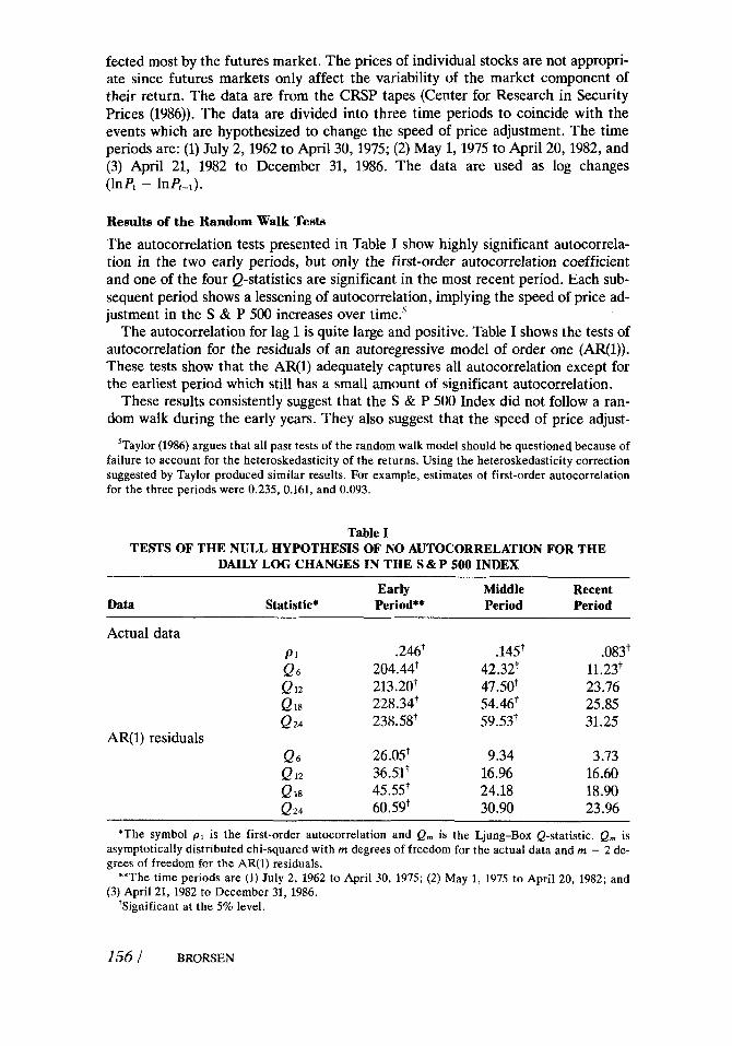
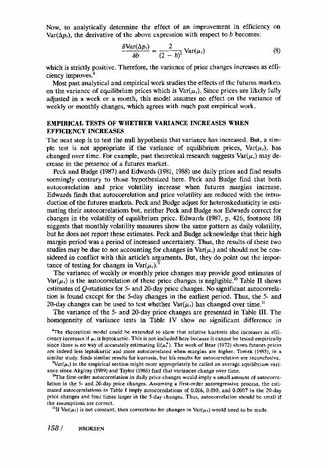
The autocorrelation tests presented in Table I show highly significant autocorrelation in the two early periods, but only the first-order autocorrelation coefficient and one of the four Q-statistics are significant in the most recent period. Each subsequent period shows a lessening of autocorrelation, implying the speed of price adjustment in the S & P 500 increases over time.'

The autocorrelation for lag 1 is quite large and positive. Table I shows the tests of autocorrelation for the residuals of an autoregressive model of order one (AR(1)). These tests show that the AR(1) adequately captures all autocorrelation except for the earliest period which still has a small amount of significant autocorrelation.

These results consistently suggest that the S & P 500 Index did not follow a random walk during the early years. They also suggest that the speed of price adjust-

5Taylor (1986) argues that all past tests of the random walk model should be questioned because of failure to account for the heteroskedasticity of the returns. Using the heteroskedasticity correction suggested by Taylor produced similar results. For example, estimates of first-order autocorrelation for the three periods were 0.235, 0.161, and 0.093.

Table I TESTS OF THE NULL HYPOTHESIS OF NO AUTOCORRELATION FOR THE

DAILY LOG CHANGES IN THE S & P 500 INDEX

Early Middle Recent Data Statistic* Period** Period Period

Actual data P I .246t .14St .083t Qs 204.44t 42.32t 11.23t Q 12 213.20t 47.50t 23.76 Q 18 228.34t 54.46t 25.85 Q 24 238.5gt 59.53+ 31.25

AR(1) residuals Q6 26.05t 9.34 3.73 Q 12 36.51t 16.96 16.60

18 45.5s 24.18 18.90 Q24 60.59t 30.90 23.96

*The symbol pl is the first-order autocorrelation and Qm is the Ljung-Box Q-statistic. Qm is asymptotically distributed chi-squared with m degrees of freedom for the actual data and m - 2 degrees of freedom for the AR(1) residuals.

**The time periods are (1) July 2, 1962 to April 30, 1975; (2) May 1, 1975 to April 20, 1982; and (3) April 21, 1982 to December 31, 1986.

'Significant at the 5% level.

ment has increased. This increase in efficiency cannot be directly linked to the deregulation of brokerage fees and the introduction of futures. But, the results are consistent with the hypothesis that these two events reduced market frictions and thus allowed faster price adjustments.

THEORETICAL RELATIONSHIP BETWEEN MARKET FRICTIONS AND PRICE VOLATILITY The theoretical work supporting the belief that futures markets may reduce volatility assumes markets are in equilibrium and thus does not hold in the short-run.6 Much of the empirical work on this issue, such as Powers (1970), Taylor and Leuthold (1974), and Figlewski (1981), uses weekly or monthly data where the equilibrium assumptions might reasonably be expected to apply.7 This article addresses a different issue, though since it looks at volatility in the short-run.

This section shows analytically the effect of reducing market frictions on the variance of price changes. First, assume equilibrium prices follow a random walk:

p : = p:-1 + p1 (2)

where prices are measured in logs, p t is equilibrium price, and where p, is an un- correlated random error term which is not necessarily normally distributed. One could assume a random walk with drift but the mean of the error term is assumed here to be zero to simplify discussion. Next, assume that due to frictions, adjustments are not instantaneous and following Nerlove (1956), prices follow a partial adjustment process:

Apt = pr - pt-1 = b(pT - pi-1) (3)

wherep, is actual price, and b is a constant which has a value between 0 and 1. This process implies the following model

Then multiplying through by (1 - bL) where L is the lag operator, eq. (4) becomes

(5 )

Eq. ( 5 ) is the AR(1) model which was argued previously to be a close approximation to the process generating daily S&P 500 values. The estimates of pl in the previous section are estimates of (1 - b). If b = 1, then adjustments are instantaneous and the process follows a random walk. Since p, and Ap,-l are independent, the variance of Ap, [Var(Ap,)] is

16)

Apt = (1 - b)Apt-1 + bpi

Var(Ap,) = (1 - b)2Var(Ap,-l) + b2Var(pl)

Var(Ap,) = b2(1 - (1 - b)’)Var(p,) = b/(2 - b)Var(p,)

Since unconditionally Var(Ap,) = Var(Apl-l) one can rewrite eq. (6) as

(7)

%ee Committee on Agriculture (1985) for a review of this literature. ’Some studies such as Simpson and Ireland (1982), Edwards (1987), and Whitakker et al. (1987) use

daily prices. Although Whitakker et al. do not recognize it, their results imply a reduction in autocorrelation and an increase in variance with the introduction of the futures market. In discussing their article, Chance (1987) argues that perhaps this is what one should expect to find.


Now, to analytically determine the effect of an improvement in efficiency on Var(Apr), the derivative of the above expression with respect to b becomes:

which is strictly positive. Therefore, the variance of price changes increases as efficiency improves.'

Most past analytical and empirical work studies the effects of the futures markets on the variance of equilibrium prices which is Var(p,), Since prices are likely fully adjusted in a week or a month, this model assumes no effect on the variance of weekly or monthly changes, which agrees with much past empirical work.

EMPIRICAL TESTS OF WHETHER VARIANCE INCREASES WHEN EFFICIENCY INCREASES The next step is to test the null hypothesis that variance has increased. But, a sim- ple test is not appropriate if the variance of equilibrium prices, Var(p,), has changed over time. For example, past theoretical research suggests Var(pJ may de- crease in the presence of a futures market.

Peck and Budge (1987) and Edwards (1981, 1988) use daily prices and find results seemingly contrary to those hypothesized here. Peck and Budge find that both autocorrelation and price volatility increase when futures margins increase. Edwards finds that autocorrelation and price volatility are reduced with the introduction of the futures markets. Peck and Budge adjust for heteroskedasticity in estimating their autocorrelations but, neither Peck and Budge nor Edwards correct for changes in the volatility of equilibrium price. Edwards (1987, p. 426, footnote 18) suggests that monthly volatility measures show the same pattern as daily volatility, but he does not report these estimates. Peck and Budge acknowledge that their high margin period was a period of increased uncertainty. Thus, the results of these two studies may be due to not accounting for changes in Var(pL,) and should not be con- sidered in conflict with this article's arguments. But, they do point out the impor- tance of testing for changes in V a r ( ~ , ) . ~

The variance of weekly or monthly price changes may provide good estimates of Var(pt) is the autocorrelation of these price changes is negligible." Table I1 shows estimates of Q-statistics for 5- and 20-day price changes. No significant autocorrelation is found except for the 5-day changes in the earliest period. Thus, the 5- and 20-day changes can be used to test whether Var(p,) has changed over time."

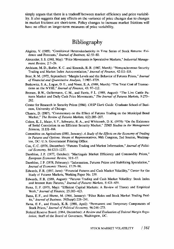
The variance of the 5- and 20-day price changes are presented in Table 111. The homogeneity of variance tests in Table IV show no significant difference in

?he theoretical model could be extended to show that relative kurtosis also increases as efficiency increases if p f is leptokurtic. This is not included here because it cannot be tested empirically since there is no way of accurately estimating E(p:). The work of Bear (1972) shows futures prices are indeed less leptokurtic and more autocorrelated when margins are higher. Tomek (1985), in a similar study, finds similar results for kurtosis, but his results for autocorrelation are inconclusive.

var(wf) in the empirical section might more appropriately be called an average equilibrium variance since Akgiray (1989) and Taylor (1986) find that variances change over time.

'?he first-order autocorrelation in daily price changes would imply a small amount of autocorrelation in the 5- and 20-day price changes. Assuming a first-order autoregressive process, the estimated autocorrelations in Table I imply autocorrelations of 0.016, 0.010, and 0.0007 in the 20-day price changes and four times larger in the 5-day changes. Thus, autocorrelation should be small if the assumptions are correct.

"If Var(pt) is not constant, then corrections for changes in Var(pf) would need to be made.

1581 BRORSEN

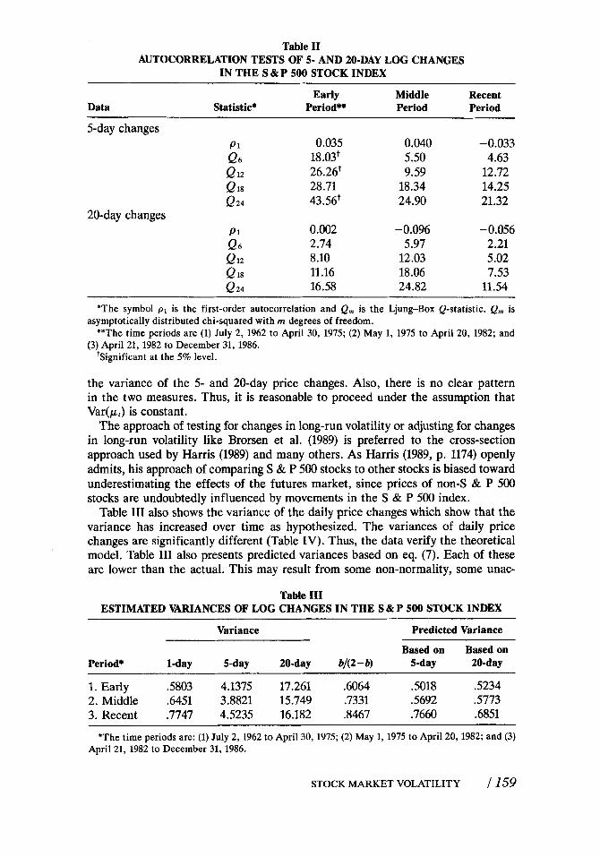
Table I1

IN THE S & P 500 STOCK INDEX AUTOCORRELATION TESTS OF 5- AND 20-DAY LOG CHANGES

Data

~ ~

Early Middle Recent Statistic* Period** Period Period

~ ~~~

5-day changes P 1 0.035 0.040 -0.033 Q 6 18.03+ 5.50 4.63 Q 12 26.26t 9.59 12.72

18 28.71 18.34 14.25 Q 24 43.56+ 24.90 21.32

20-day changes P 1 0.002 -0.096 -0.056 Q 6 2.74 5.97 2.21

Q i s 11.16 18.06 7.53 Q 12 8.10 12.03 5.02

Q 24 16.58 24.82 11.54

*The symbol pl is the first-order autocorrelation and Qm is the Ljung-Box Q-statistic. Qm is

**The time periods are (1) July 2, 1962 to April 30, 1975; (2) May 1, 1975 to April 20, 1982; and

'Significant at the 5% level.

asymptotically distributed chi-squared with rn degrees of freedom.

(3) April 21, 1982 to December 31, 1986.

the variance of the 5- and 20-day price changes. Also, there is no clear pattern in the two measures. Thus, it is reasonable to proceed under the assumption that Var(pt) is constant.

The approach of testing for changes in long-run volatility or adjusting for changes in long-run volatility like Brorsen et al. (1989) is preferred to the cross-section approach used by Harris (1989) and many others. As Harris (1989, p. 1174) openly admits, his approach of comparing S & P 500 stocks to other stocks is biased toward underestimating the effects of the futures market, since prices of non-S & P 500 stocks are undoubtedly influenced by movements in the S & P 500 index.

Table I11 also shows the variance of the daily price changes which show that the variance has increased over time as hypothesized. The variances of daily price changes are significantly different (Table IV). Thus, the data verify the theoretical model. Table I11 also presents predicted variances based on eq. (7). Each of these are lower than the actual. This may result from some non-normality, some unac-

Table I11 ESTIMATED VARIANCES OF LOG CHANGES IN THE S & P 500 STOCK INDEX

Variance Predicted Variance

Based on Based on Period* 1-day 5-day 20-day b/(2-b) 5-day 20-day

1. Early 3303 4.1375 17.261 .6064 .5018 S234 2. Middle .6451 3.8821 15.749 .7331 S692 s773 3, Recent .7747 4.5235 16.182 .8467 .7660 .6851

*The time periods are: (1) July 2, 1962 to April 30, 1975; (2) May 1,1975 to April 20, 1982; and (3) April 21, 1982 to December 31, 1986.


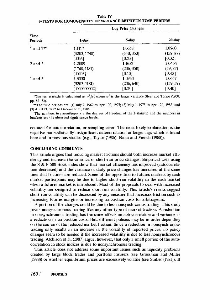
Table IV F-TESTS FOR HOMOGENEITY OF VARIANCE BETWEEN TIME PERIODS

Log Price Changes

Time Periods l-day 5-day 20-day

1 and 2** 1.1117 (3203,1748)+ [ -0061

2 and 3 1.2009 (1748,1181) [ .OO03]

1 and 3 1.3350 (3203,1181) [ .OO0000002]

1.0658 (640,350) [0.25] 1.1652 (236,350)

1.0933 (236,640)

[0.10]

[0.20]

1.0960 (159,87) [0.32] 1.0454

E0.421 1.0667 (159,59) [0.40]

(59787)

*The test statistic is calculated as (rt/cr: where a: is the larger variance Steel and Torrie (1960,

**The time periods are: (1) July 2, 1962 to April 30, 1975; (2) May 1, 1975 to April 20, 1982; and

'The numbers in parentheses are the degrees of freedom of the F-statistic and the numbers in

pp. 82-83).

(3) April 21, 1982 to December 31, 1986.

brackets are the observed significance levels.

counted for autocorrelation, or sampling error. The most likely explanation is the negative but statistically insignificant autocorrelation at longer lags which is found here and in previous studies (e.g., Taylor (1986); Fama and French (1988)).

CONCLUDING COMMENTS This article argues that reducing market frictions should both increase market efficiency and increase the variance of short-run price changes. Empirical tests using the S & P 500 stock index show that market efficiency has improved (autocorrelation decreased) and the variance of daily price changes has increased at the same time that frictions are reduced. Some of the opposition to futures markets by cash market participants may be due to higher short-run volatility in the cash market when a futures market is introduced. Most of the proposals to deal with increased volatility are designed to reduce short-run volatility. This article's results suggest short-run volatility can be decreased by any measure that increases friction such as increasing futures margins or increasing transaction costs for arbitrageurs.

A portion of the changes could be due to less nonsynchronous trading. This study treats nonsynchronous trading like any other type of market friction. A reduction in nonsynchronous trading has the same effects on autocorrelation and variance as a reduction in transaction costs. But, different policies may be in order depending on the source of the reduced market friction. Since a reduction in nonsynchronous trading only results in an increase in the volatility of reported prices, no policy changes seem to be needed if the increased volatility is due to less nonsynchronous trading. Atchison et al. (1987) argue, however, that only a small portion of the autocorrelation in stock indices is due to nonsynchronous trading.

This article does not address some important issues such as liquidity problems created by large block trades and portfolio insurers (see Grossman and Miller (1988)) or whether equilibrium prices are excessively volatile (see §hiller (1981)). It

160/ BRORSEN

simply argues that there is a tradeoff between market efficiency and price variability. It also suggests that any effects on the variance of price changes due to changes in market frictions are short-term. Policy changes to increase market frictions will have no effect on longer-term measures of price variability.

Bibliography Akgiray, V. (1989): “Conditional Heteroskedasticity in Time Series of Stock Returns: Evi-

dence and Forecasts,” Journal of Business, 62:55-80. Alexander, S . S. (1961, May): “Price Movements in Speculative Markets,” Industrial Manage-

ment Review, 2:7-26. Atchison, M. D., Butler, K. C. and Simonds, R. R. (1987, March): “Nonsynchronous Security

Trading and Market Index Autocorrelation,” Journal of Finance, 42:lll-118. Bear, R. M. (1972, September): “Margin Levels and the Behavior of Futures Prices,” Journal

of Financial and Quantitative Analysis, 7:1907-1729. Berkowitz, S. A., Logue, D. E., and Noser, E. A. (1988, March): “The Total Cost of Transac-

tions on the NYSE,” Journal of Finance, 43: 97-112. Brorsen, B.W., Oellermann, C. M., and Farris, P. L. (1989, August): “The Live Cattle Fu-

tures Market and Daily Cash Price Movements,” The Journal of Futures Markets, 9:273- 282.

Center for Research in Security Prices (1986). CRSP User’s Guide. Graduate School of Busi- ness, University of Chicago.

Chance, D. (1987). “Commentary on the Effect of Futures Trading on the Municipal Bond Market,” The Review of Futures Markets, 6(2):205-207.

Cohen, K. J., Maier, S. F., Schwartz, R. A., and Whitcomb, D. K. (1979): “On the Existence of Serial Correlation in an Efficient Security Market,” TIMS Studies in the Management Sciences, 11:151-168.

Committee on Agriculture (1985, January): A Study of the Effects on the Economy of Trading in Futures and Options. House of Representatives, 98th Congress, 2nd Session, Washing- ton, DC: U. S. Government Printing Office.

Cox, C. C. (1976, December): “Futures Trading and Market Information,” Journal of Politi- cal Economy, 84:1215-1237.

Danthine, J. P. (1977, October): “Martingale Market Efficiency and Commodity Prices,’’ European Economic Review, 1O:l-17.

Danthine, J. P. (1978, February): “Information, Futures Prices and Stabilizing Speculation,” Journal of Economic Theory, 17:79-98.

Edwards, F. R. (1987, June): “Financial Futures and Cash Market Volatility,” Center for the Study of Futures Markets, Working Paper No. 159.

Edwards, F. R. (1988, August): “Futures Trading and Cash Market Volatility: Stock Index and Interest Rate Futures,” Journal of Futures Markets, 8:421-439.

Fama, E.F. (1970, May): “Efficient Capital Markets: A Review of Theory and Empirical Work,” Journal of Finance, 25:383-423.

Fama, E. F., and Blume, M. (1966, January): “Filter Rules and Stock Market Trading Prof- its,” Journal of Business, 39(Suppl):226-241.

Fama, E. F., and French, K. R. (1988, April): “Permanent and Temporary Components of Stock Prices,” Journal of Political Economy, 96:246-273.

Federal Reserve Board. (1984, December): A Review and Evaluation of Federal Margin Regu- lation, Staff of the Board of Governors, Washington, DC.

STOCK MARKET VOLATILITY J 161

Figlewski, S. (1981, May): “GNMA Passthrough Securities: Futures Trading and Volatility in

Fisher, L. (1966, January): “Some New Stock Market Indexes,” Journal of Business,

Garbade, H . D., and Silber, W. L. (1983, May): “Price Movements and Price Discovery in

Grossman, S. J., and Miller, M. H. (1988, July): “Liquidity and Market Structure,” Journal of

Harris, L. (1989, December): “S & P 500 Cash Stock Price Volatilities,” Journal of Finance

Herbst, A. F., McCormack, J. P., and West, E. N. (1987, August): “Investigation of a Lead- Lag Relationship Between Spot Stock Indices and Their Futures Contracts,” Journal of Futures Markets, 7:373-381.

Kawaller, I. G., Koch, P. D., and Koch, T.W. (1987, December): “The Temporal Price Rela- tionship Between S & P 500 Futures and the S & P 500 Index,” Journal of Finance,

LeBaron, B. (1989, November): “Some Relations Between Volatility and Serial Correlations in Stock Market Returns,” University of Wisconsin-Madison, Department of Economics, unpublished working paper.

Ljung, G. M., and Box, G. E. P. (1978): “On a Measure of Lack of Fit in Time Series Mod- els,” Biometrika, 65:297-303.

Lo, A.W., and Craig Mackinlay, A. ‘#n Econometric Analysis of Nonsynchronous Trading.” Working paper 3003-89-EFA, Sloan School of Management, Massachusetts Institute of Technology, Cambridge, MA.

Nerlove, M. (1956): “Estimates of the Elasticities of Supply of Selected Agricultural Com- modities,” Journal of Farm Economics, 38:496-509.

Ng, N. (1987): “Detecting Spot Price Forecasts in Futures Prices Using Causality Tests,” Re- view of Futures Markets, 6(2):250-267.

Peck, A. E., Budge, C. C. (1987): “The Effects of Extraordinary Speculative Margins in the 1947-48 Grain Futures Markets,” Food Research Institute Studies, 20(2):165-180.

Perry, P. R. (1985, December): “Portfolio Serial Correlation and Nonsynchronous Trading,” Journal of Financial and Quantitative Analysis, 20:517-523.

Powers, M. J. (1970, June): “Does Futures Trading Reduce Price Fluctuations in the Cash Market?” American Economic Review, 60:460-464.

Report of the Presidential Task Force on Market Mechanisms. (1988, January): Washington, DC:U.S. Government Printing Office.

Scholes, M. and Williams, J. (1977, December): “Estimating Betas from Nonsynchronous Data,” Journal of Financial Economics, 5:309-327.

Shiller, R. J. (1981, June): “Do Stock Prices Move Too Much to be Justified by Subsequent Changes in Dividends?” American Economic Review, 71:421-436.

Silber, W. L. (1984, September): “Marketmaker Behavior in an Auction Market: An Analysis of Scalpers in Futures Markets,” Journal of Finance, 39:937-953.

Simpson, W.G., and Ireland, T.C. (1982): “The Effect of Futures Trading on the Price Volatility of GNMA Securities,” Journal of Futures Markets, 2(4):357-366.

Steel, R. G. D., and Torrie, J. H. (1960): Principles and Procedures of Statistics. New York: McGraw-Hill Book Co.

Taylor, G. S. , and Leuthold, R. M. (1974, February): “The Influence of Futures Trading on Cash Cattle Price Variations,” Food Research Institute Studies, 13:29-35.

Taylor, S. J. (1986): Modeling Financial Time Series. Chichester: John Wiley & Sons.

the GNMA Market,” Journal of Finance, 36:445-456.

39~191-225.

Futures and Cash Markets,” Review of Economics and Statistics, 65:289-297.

Finance, 43 : 617-633.

44~1155-1175.

42~1309-1329.

162/ BRORSEN

Tomek, W. G. (1985): “Margins on Futures Contracts: Their Economic Roles and Regula- tion.” In Futures Markets: Regulatory Issues, Peck, A. E. (ed.). Washington, DC: American Enterprise Institute for Public Policy Research.

Whitakker, G., Bowyer, L. E., and Klein, D. P. (1987): “The Effect of Futures Trading on the Municipal Bond Market,” Review of Futures Markets, 6(2):196-204.


futures trading, transaction costs, and stock market volatility

Documents