fundamentals of statistical signal processing(1) · introduction signal spectral analysis:...
TRANSCRIPT

Lesson 9

Introduction Signal Spectral Analysis: Estimation of the power spectral
density
The problem of spectral estimation is very large and has applications very different from each other
Applications: To study the vibrations of a system
To study the stability of the frequency of a oscillator
To estimate the position and number of signal sources in an acoustic field
To estimate the parameters of the vocal tract of a speaker
Medical diagnosis
Control system design
In general To estimate and predict signals in time or in space
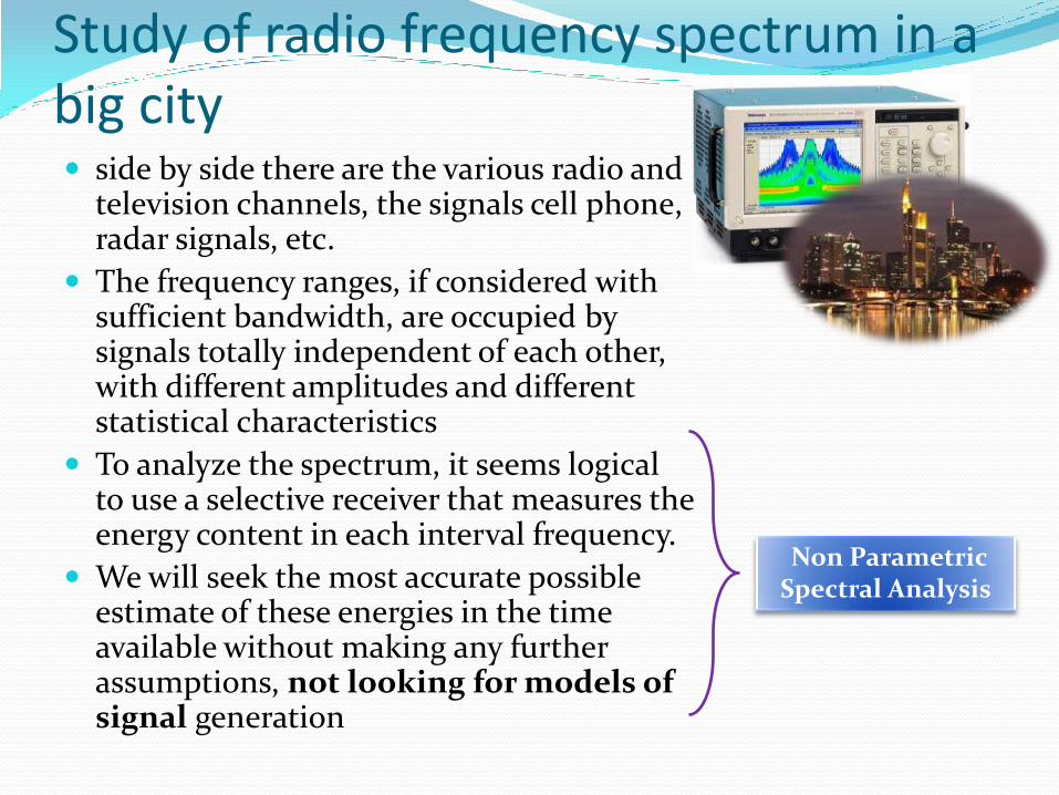
Study of radio frequency spectrum in a big city side by side there are the various radio and
television channels, the signals cell phone, radar signals, etc.
The frequency ranges, if considered with sufficient bandwidth, are occupied by signals totally independent of each other, with different amplitudes and different statistical characteristics
To analyze the spectrum, it seems logical to use a selective receiver that measures the energy content in each interval frequency.
We will seek the most accurate possible estimate of these energies in the time available without making any further assumptions, not looking for models of signal generation
Non Parametric Spectral Analysis
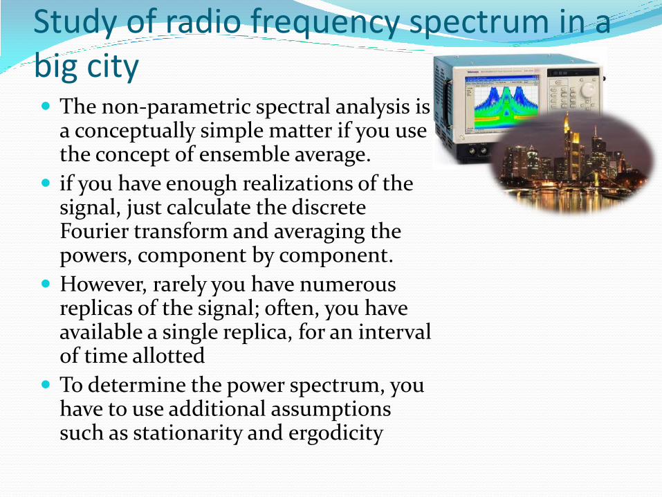
Study of radio frequency spectrum in a big city The non-parametric spectral analysis is
a conceptually simple matter if you use the concept of ensemble average.
if you have enough realizations of the signal, just calculate the discrete Fourier transform and averaging the powers, component by component.
However, rarely you have numerous replicas of the signal; often, you have available a single replica, for an interval of time allotted
To determine the power spectrum, you have to use additional assumptions such as stationarity and ergodicity

Analysis of the speech signal consider the spectrum of acoustic signal due
to vibration or a voice signal
in this case, all of the signal as a whole has unique origins and then there will be the relationship between the contents of the various spectral bands.
it must first choose a model for the generation of the signal and then determine the parameters of the model itself
For example, it will seek the parameters of a linear filter that, powered by a uniform spectrum signal (white noise) produces a power spectrum similar to the spectrum under analysis
Parametric Spectral Analysis
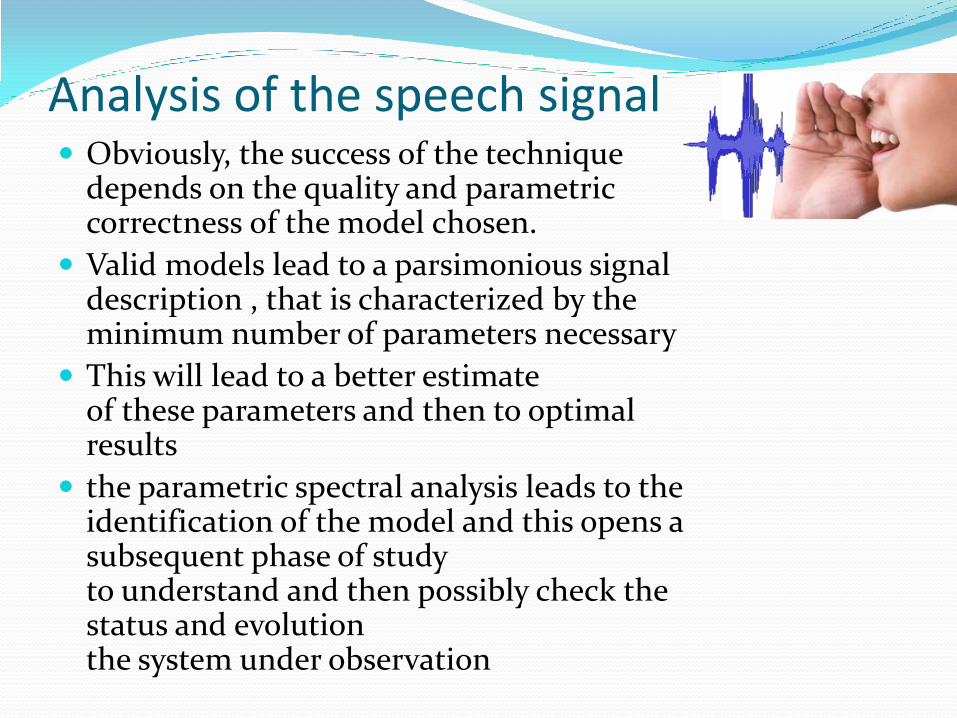
Analysis of the speech signal Obviously, the success of the technique
depends on the quality and parametric correctness of the model chosen.
Valid models lead to a parsimonious signal description , that is characterized by the minimum number of parameters necessary
This will lead to a better estimate of these parameters and then to optimal results
the parametric spectral analysis leads to the identification of the model and this opens a subsequent phase of study to understand and then possibly check the status and evolution the system under observation
Formal Problem Definition Let be y= {y(1), y(2), . . . , y(N)} a second order
stationary random process,
GOAL: to determine an estimate of its power spectral density for ω ∈ [−π, +π]
Observation
We want
The main limitation on the quality of most PSD estimates is due to the quite small number of data samples N usually available
Most commonly, N is limited by the fact that the signal under study can be considered wide sense stationary only over short observation intervals
)(ˆ
)(
0|)()(ˆ|
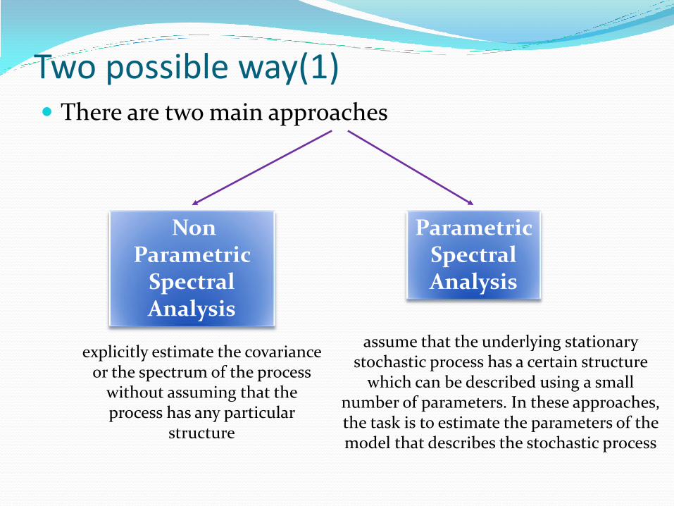
Two possible way(1) There are two main approaches
Non Parametric
Spectral Analysis
Parametric Spectral Analysis
explicitly estimate the covariance or the spectrum of the process
without assuming that the process has any particular
structure
assume that the underlying stationary stochastic process has a certain structure
which can be described using a small number of parameters. In these approaches, the task is to estimate the parameters of the model that describes the stochastic process
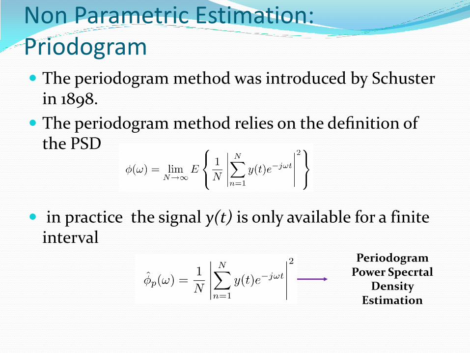
Non Parametric Estimation: Priodogram The periodogram method was introduced by Schuster
in 1898.
The periodogram method relies on the definition of the PSD
in practice the signal y(t) is only available for a finite interval
Periodogram Power Specrtal
Density Estimation
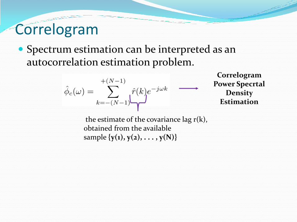
Correlogram Spectrum estimation can be interpreted as an
autocorrelation estimation problem. Correlogram
Power Specrtal Density
Estimation
the estimate of the covariance lag r(k), obtained from the available sample {y(1), y(2), . . . , y(N)}

Estimation of Autocorrelation Sequence(ACS) There are two standard way to obtain an estimate
unbiased estimate
biased estimate
Both estimators respect the symmetry properties of the ACS The biased estimate is usually preferred, for the following reasons:
the ACS sequence decays rather rapidly so that r(k) is quite small for large lags k
the ACS sequence is guaranteed to be positive semidefinite. is not the
case for the unbised definition if the biased ACS estimator is used in the estimation the correlogram is
eqaul to the periodogramm
)(ˆ kr
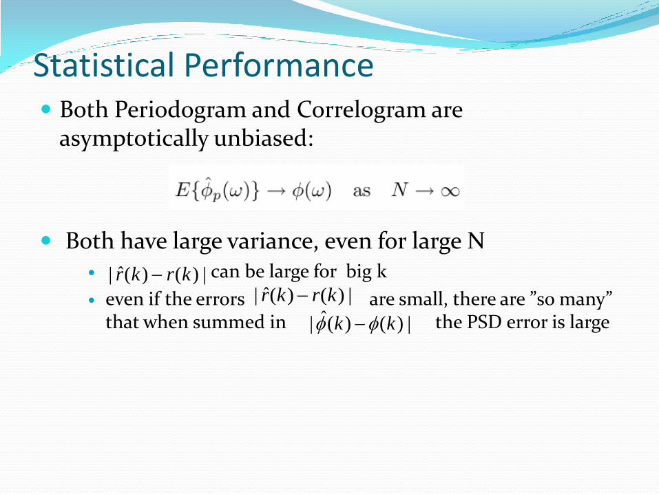
Statistical Performance Both Periodogram and Correlogram are
asymptotically unbiased:
Both have large variance, even for large N can be large for big k
even if the errors are small, there are ”so many” that when summed in the PSD error is large
|)()(ˆ| krkr |)()(ˆ| krkr
|)()(ˆ| kk

Periodogram Bias
Bartlett window.
Frequency Domain

Bartlett window Ideally, to have zero bias, we
want WB(ω) = Dirac impulse δ(ω)
The main lobe width decreases as 1/N.
For small values of N, WB(ω) may differ quite a bit from δ(ω)
If the unbised estimation the window is rectangular
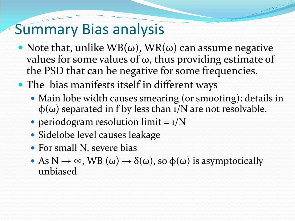
Summary Bias analysis Note that, unlike WB(ω), WR(ω) can assume negative
values for some values of ω, thus providing estimate of the PSD that can be negative for some frequencies.
The bias manifests itself in different ways Main lobe width causes smearing (or smooting): details in
φ(ω) separated in f by less than 1/N are not resolvable.
periodogram resolution limit = 1/N
Sidelobe level causes leakage
For small N, severe bias
As N → ∞, WB (ω) → δ(ω), so φ(ω) is asymptotically unbiased

Periodogram Variance As N → ∞
inconsistent estimate
erratic behavior
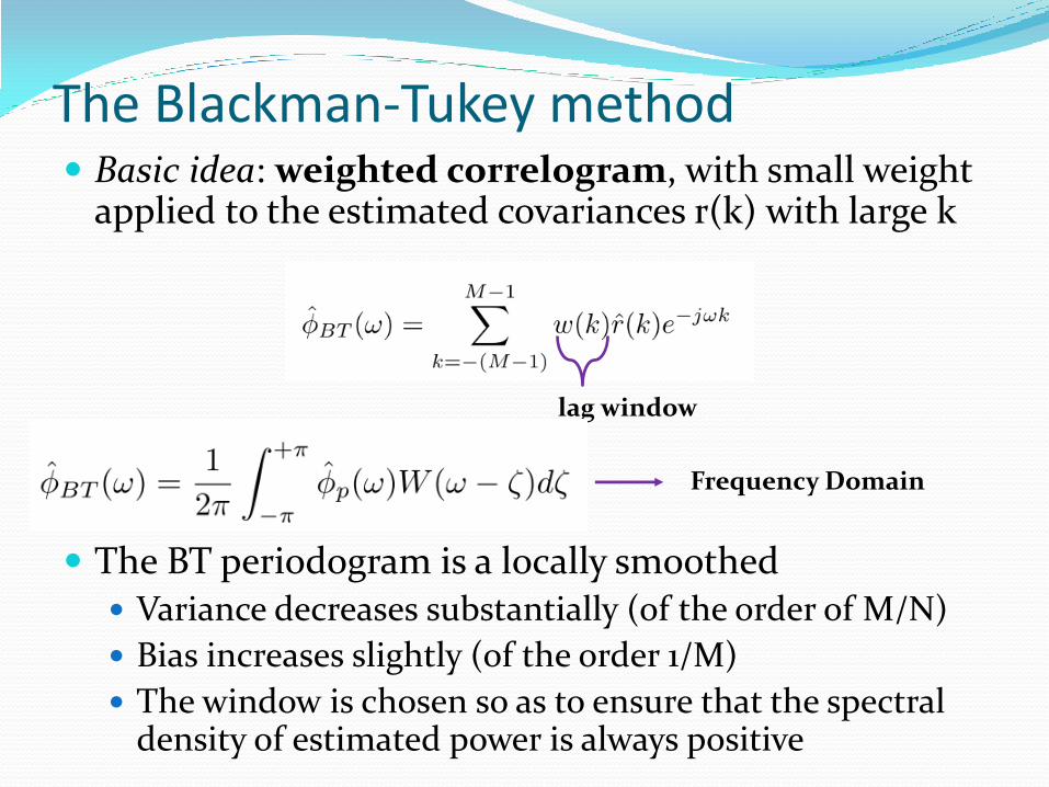
The Blackman-Tukey method Basic idea: weighted correlogram, with small weight
applied to the estimated covariances r(k) with large k
The BT periodogram is a locally smoothed Variance decreases substantially (of the order of M/N)
Bias increases slightly (of the order 1/M)
The window is chosen so as to ensure that the spectral density of estimated power is always positive
lag window
Frequency Domain
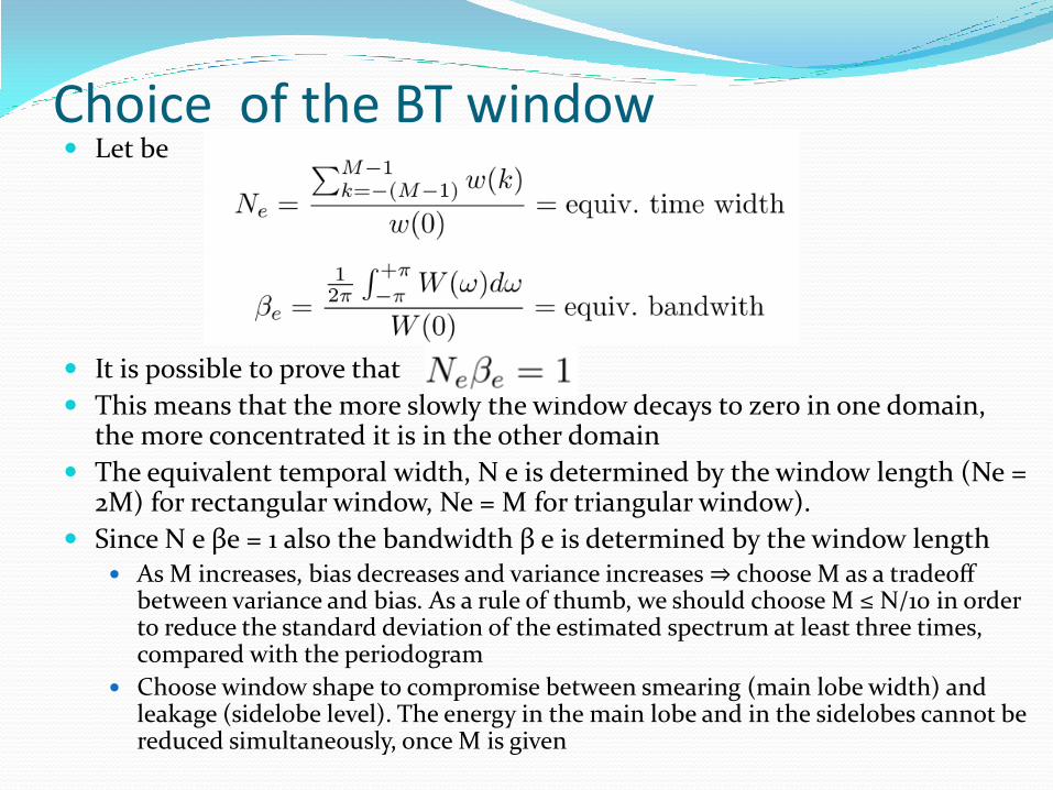
Let be
It is possible to prove that
This means that the more slowly the window decays to zero in one domain, the more concentrated it is in the other domain
The equivalent temporal width, N e is determined by the window length (Ne = 2M) for rectangular window, Ne = M for triangular window).
Since N e βe = 1 also the bandwidth β e is determined by the window length As M increases, bias decreases and variance increases ⇒ choose M as a tradeoff
between variance and bias. As a rule of thumb, we should choose M ≤ N/10 in order to reduce the standard deviation of the estimated spectrum at least three times, compared with the periodogram
Choose window shape to compromise between smearing (main lobe width) and leakage (sidelobe level). The energy in the main lobe and in the sidelobes cannot be reduced simultaneously, once M is given
Choice of the BT window
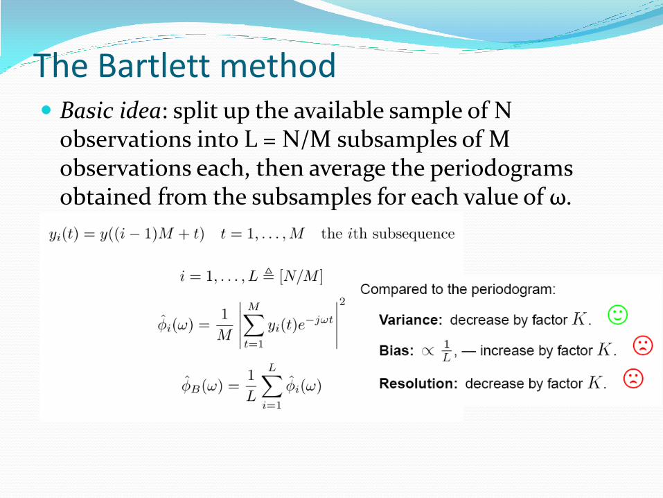
The Bartlett method Basic idea: split up the available sample of N
observations into L = N/M subsamples of M observations each, then average the periodograms obtained from the subsamples for each value of ω.
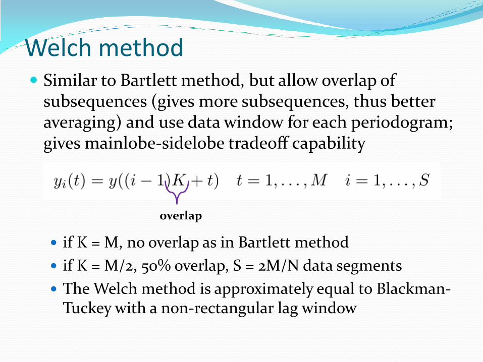
Welch method Similar to Bartlett method, but allow overlap of
subsequences (gives more subsequences, thus better averaging) and use data window for each periodogram; gives mainlobe-sidelobe tradeoff capability
if K = M, no overlap as in Bartlett method
if K = M/2, 50% overlap, S = 2M/N data segments
The Welch method is approximately equal to Blackman-Tuckey with a non-rectangular lag window
overlap
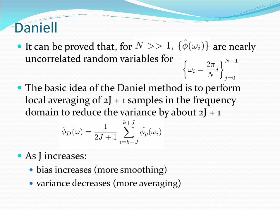
Daniell It can be proved that, for are nearly
uncorrelated random variables for
The basic idea of the Daniel method is to perform local averaging of 2J + 1 samples in the frequency domain to reduce the variance by about 2J + 1
As J increases:
bias increases (more smoothing)
variance decreases (more averaging)
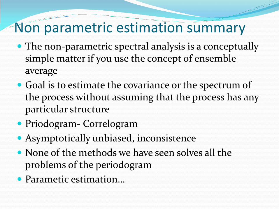
Non parametric estimation summary The non-parametric spectral analysis is a conceptually
simple matter if you use the concept of ensemble average
Goal is to estimate the covariance or the spectrum of the process without assuming that the process has any particular structure
Priodogram- Correlogram
Asymptotically unbiased, inconsistence
None of the methods we have seen solves all the problems of the periodogram
Parametic estimation…

Matlab Examples: Periodogram
Exercise 1.a
Estimate the power spectral density of the signal “flute2” by means of periodogram
Hint on periodogram:
the spectrum estimation using periodogram is given by the following equation
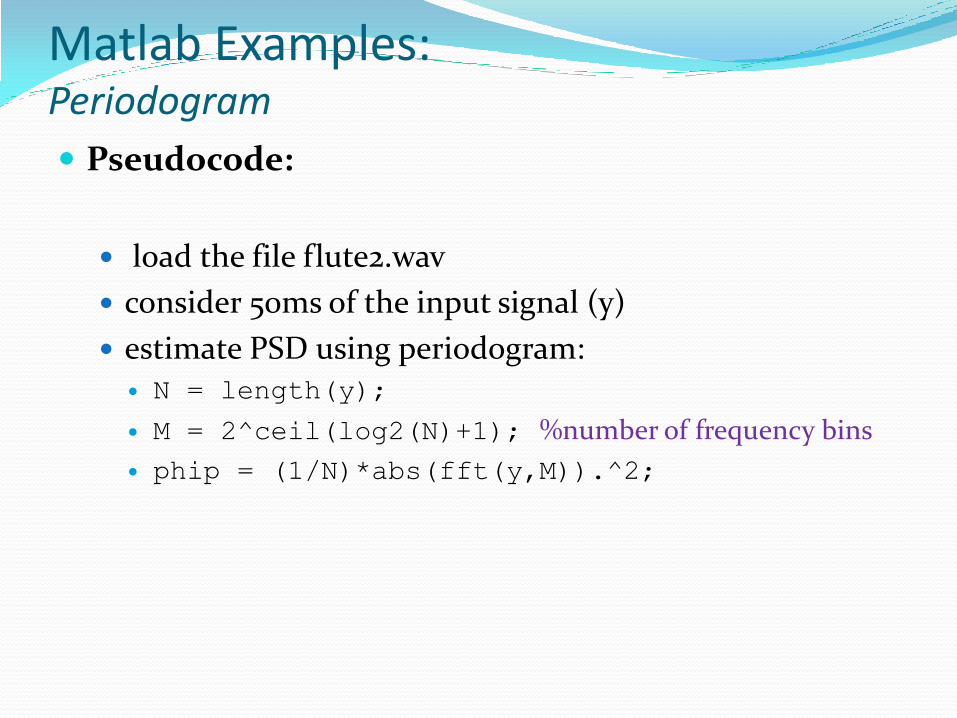
Matlab Examples: Periodogram
Pseudocode:
load the file flute2.wav
consider 50ms of the input signal (y)
estimate PSD using periodogram: N = length(y);
M = 2^ceil(log2(N)+1); %number of frequency bins
phip = (1/N)*abs(fft(y,M)).^2;

Matlab Examples: Periodogram

Exercise 1.b
Quantify the bias and variance of the periodogram
Hint on periodogram:
Periodogram is asymptotically unbiased and has large variance, even for large N.
Matlab Examples: Bias and variance of the periodogram
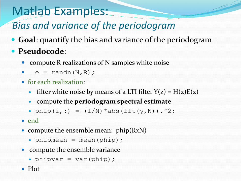
Goal: quantify the bias and variance of the periodogram
Pseudocode:
compute R realizations of N samples white noise
e = randn(N,R);
for each realization:
filter white noise by means of a LTI filter Y(z) = H(z)E(z)
compute the periodogram spectral estimate
phip(i,:) = (1/N)*abs(fft(y,N)).^2;
end
compute the ensemble mean: phip(RxN)
phipmean = mean(phip);
compute the ensemble variance
phipvar = var(phip);
Plot
Matlab Examples: Bias and variance of the periodogram

Matlab Examples: Bias and variance of the periodogram
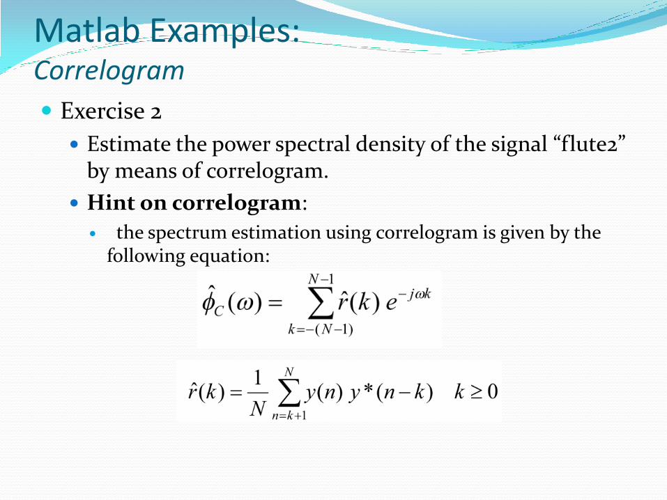
Matlab Examples: Correlogram
Exercise 2
Estimate the power spectral density of the signal “flute2” by means of correlogram.
Hint on correlogram:
the spectrum estimation using correlogram is given by the following equation:

Matlab Examples: Correlogram Goal: Estimate the power spectral density using the correlogram
Pseudocode:
load the file flute2.wav
consider 50ms of the input signal (y)
estimate ACS
[r lags] = xcorr(y, 'biased');
r = circshift(r,N);
estimate PSD using correlogram:
N = length(y);
M = 2^ceil(log2(2*N-1)+1); %number of frequency bins
phic = fft(r,M);

Matlab Examples: Correlogram
MATLAB Hint: Matlab provides the functions:
[r lag]=xcorr(x,’biased’) that produces a biased estimate of the autocorrelation (2N-1 samples) of the stationary sequence “x”. “lag” is the vector of lag indices [-N+1:1:N-1].
r = circshift(r,N) that circularly shifts the values in the array r by N elements. If N is positive, the values of r are shifted down (or to the right). If it is negative, the values of r are shifted up (or to the left).
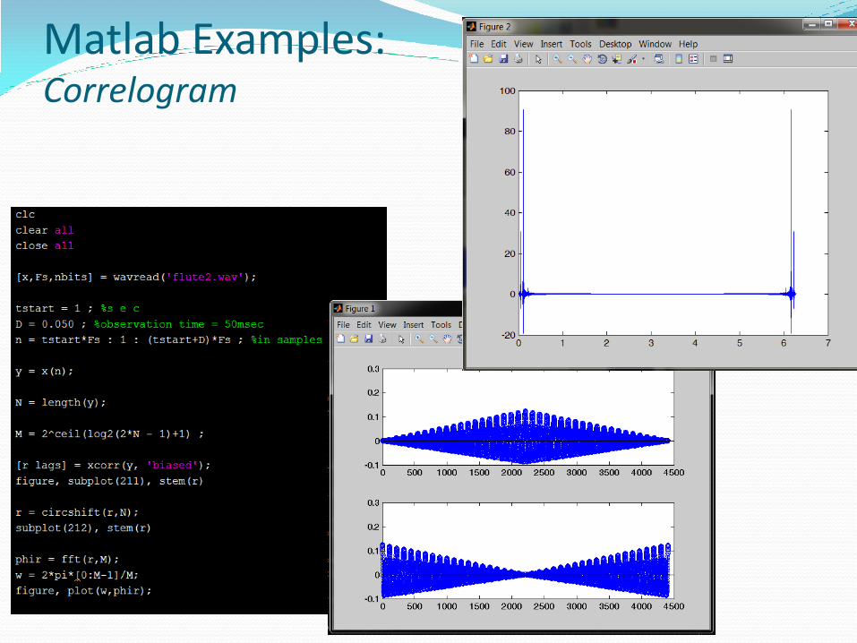
Matlab Examples: Correlogram
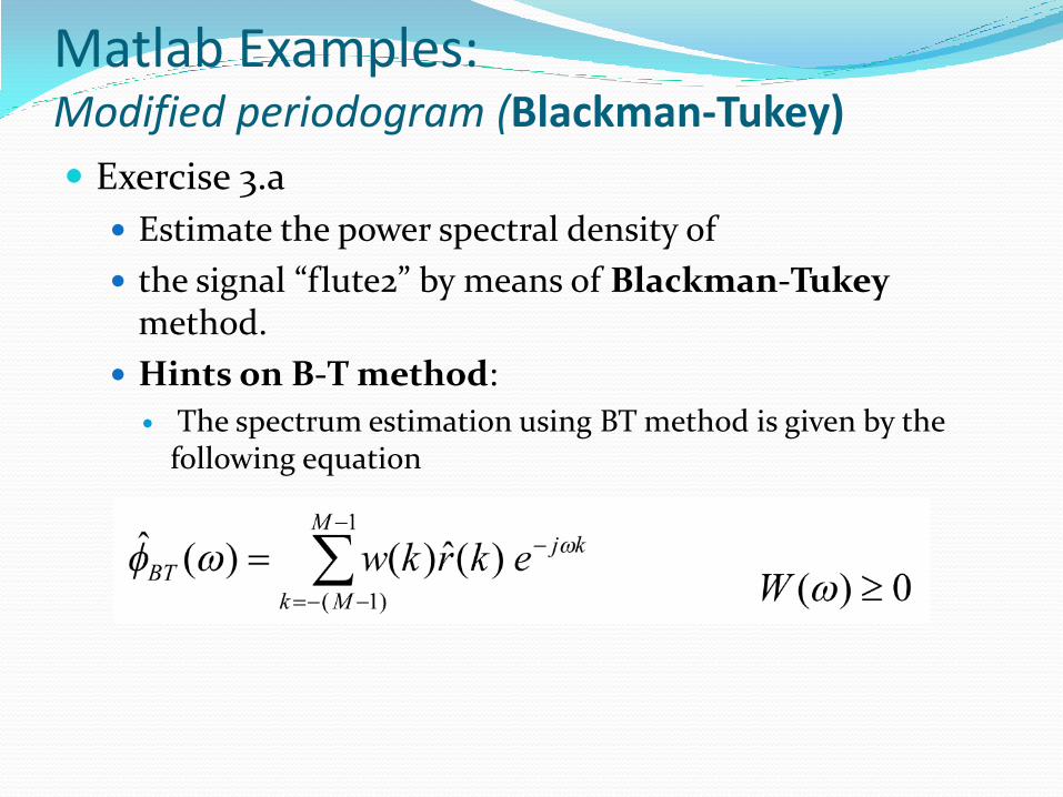
Matlab Examples: Modified periodogram (Blackman-Tukey)
Exercise 3.a
Estimate the power spectral density of
the signal “flute2” by means of Blackman-Tukey method.
Hints on B-T method:
The spectrum estimation using BT method is given by the following equation
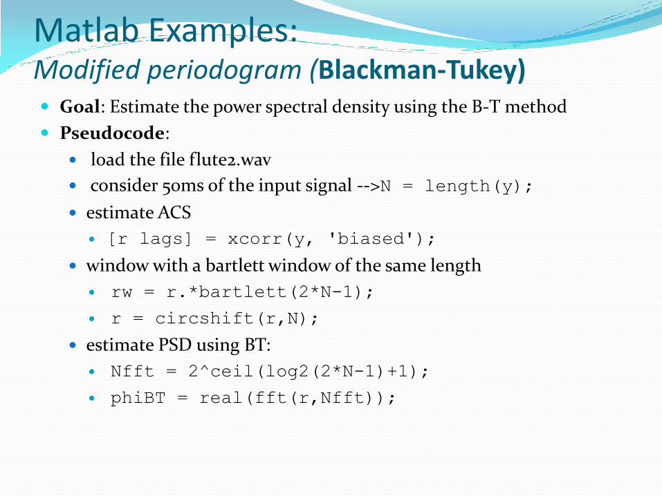
Goal: Estimate the power spectral density using the B-T method
Pseudocode:
load the file flute2.wav
consider 50ms of the input signal -->N = length(y);
estimate ACS
[r lags] = xcorr(y, 'biased');
window with a bartlett window of the same length
rw = r.*bartlett(2*N-1);
r = circshift(r,N);
estimate PSD using BT:
Nfft = 2^ceil(log2(2*N-1)+1);
phiBT = real(fft(r,Nfft));
Matlab Examples: Modified periodogram (Blackman-Tukey)
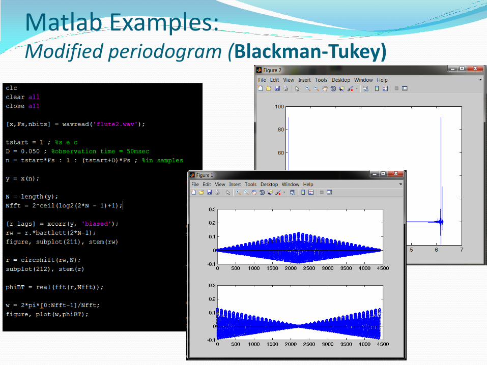
Matlab Examples: Modified periodogram (Blackman-Tukey)

Matlab Examples: Modified periodogram (Blackman-Tukey) Exercise 3.b
Goal: quantify the bias and variance of the BT method
Pseudocode:
compute R realizations of N samples white noise
e = randn(N,R);
for each realization:
filter white noise by means of a LTI filter Y(z) = H(z)E(z)
compute the BT spectral estimate
end
compute the ensemble mean: phip(RxN)
phipmean = mean(phip);
compute the ensemble variance
phipvar = var(phip);
Plot
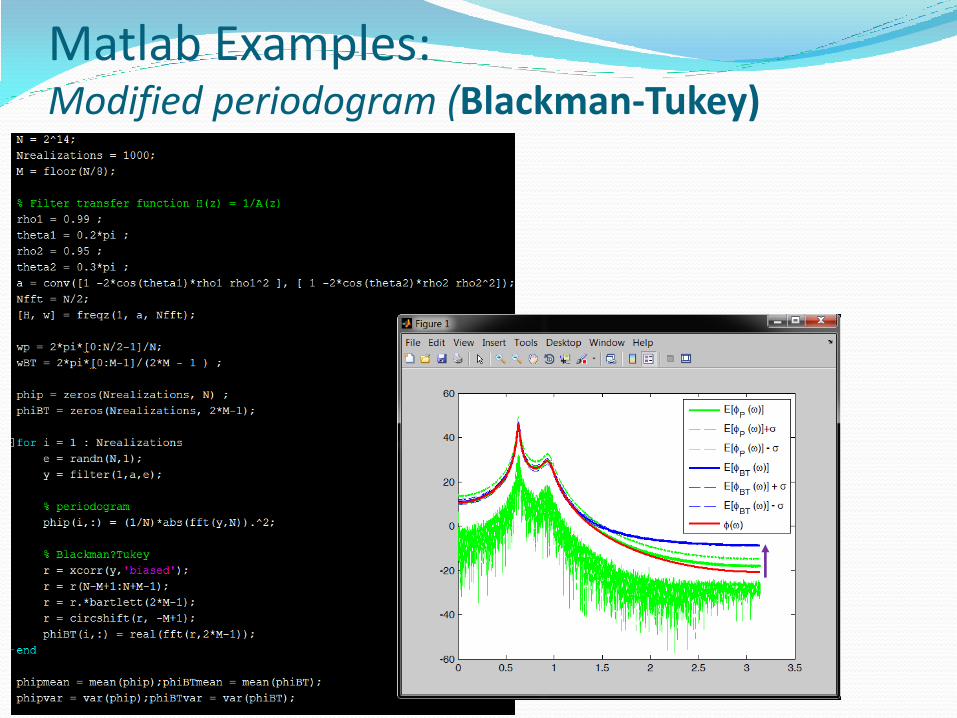
Matlab Examples: Modified periodogram (Blackman-Tukey)
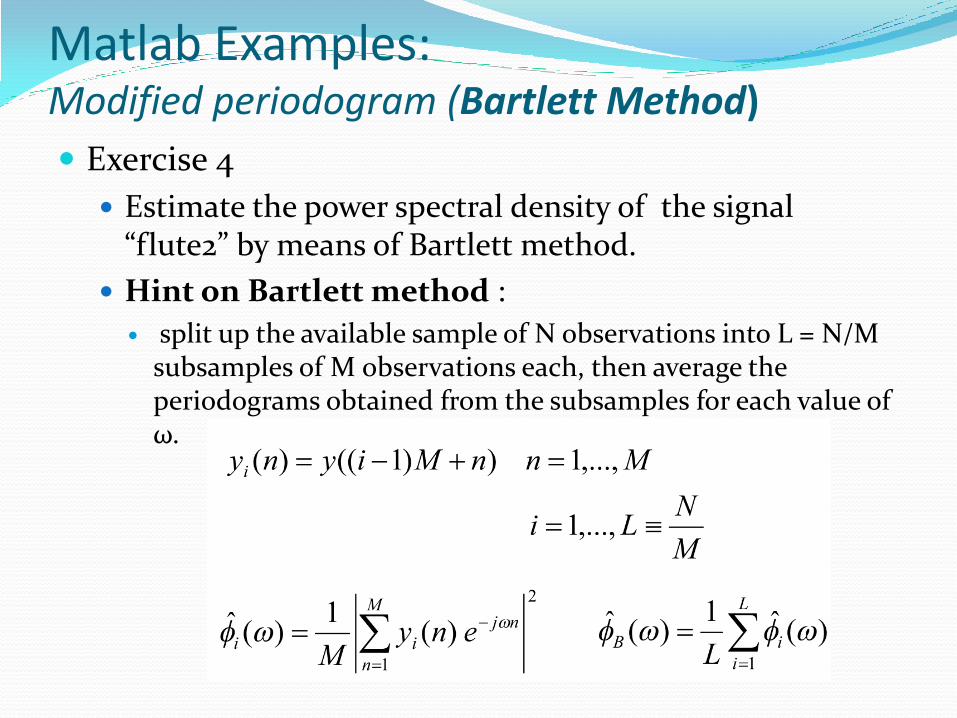
Matlab Examples: Modified periodogram (Bartlett Method)
Exercise 4
Estimate the power spectral density of the signal “flute2” by means of Bartlett method.
Hint on Bartlett method :
split up the available sample of N observations into L = N/M subsamples of M observations each, then average the periodograms obtained from the subsamples for each value of ω.

Matlab Examples: Modified periodogram (Bartlett Method) Goal: Estimate the power spectral density using the Baralett Method
Pseudocode:
load the file flute2.wav
consider 50ms of the input signal -->N = length(y);
define the number of subsequences L and the number of samples for each of them M=ceil(N/L)
for each subsequence:
consider the right samples: yl = y(1+l*M : M+l*M);
estimate periodogram: (1/M)*abs(fft(yl)).^2
mean periodograms of the subsequences:
phil = phil + (1/M)*abs(fft(yl)).^2;
phiB=phil/L;
end

Matlab Examples: Modified periodogram (Bartlett Method)

Matlab Examples: Modified periodogram (Welch Method)
Exercise 5
Estimate the power spectral density of the signal “flute2” by means of Welch method.
Hint on Welch method :
similar to Bartlett method but: allow overlap of subsequences use data window for each periodogram

Matlab Examples: Modified periodogram (Welch Method) Goal: Estimate the power spectral density using the Baralett Method
Pseudocode:
load the file flute2.wav
consider 50ms of the input signal -->N = length(y);
define: the number of samples for each subsequence: M
the number of new samples for each subsequence: K=M/4 the number of subsequences: S= N/K - (M-K)/K;
the window: v = hamming(M) ;
P = (1/M)*sum(v.^2);
for each subsequence
consider the right samples: xs = x(1+s*K : M+s*K) ;
window the subsequence: v.*xs
estimate periodogram: (1/(M*P))*abs(fft(v.*xs)).^2 mean periodograms of the subsequences:
phis = phis+ (1/(M*P))*abs(fft(v.*xs)).^2 ;
phiW = phis/S;
end

Matlab Examples: Modified periodogram (Welch Method)

Parametric Spectral Estimation Consider a sequence of independent samples {xn} and
with it feeding a filter H(ω), if the transform of the sequence {xn} is indicated X(ω), the output will be:
The power spectral density of the process white {xn} is constant because for sequences of independent samples of length N, the components of the discrete Fourier transform are all of equal value root mean square (assuming T = 1):

Parametric Spectral Estimation The parametric spectral analysis consists in determining the
parameters of the filter H (ω) in such a way that the spectrum in the filter output resembles as much as possible to the spectrum of the signal {yn} analyzed
We will have spectral analysis Moving Average (MA) if the filter has a z-transform characterized by all zeros
We have the case Auto Regressive (AR) when The filter is all-pole autoregressive
We have the mixed case ARMA (Auto Regressive Moving Average) in the more general case of poles and zeros.
We will see that the parametric spectral analysis all zeros practically coincides with the modified non parametric techniques.
The spectral techniques AR instead are of very different nature and innovative
The spectral analysis ARMA then, is less frequently used also because as is known, any filter can be represented with only zeros or only poles and a mixed representation serves only for a description of the same (or a similar) transfer function with a lower number of parameters.
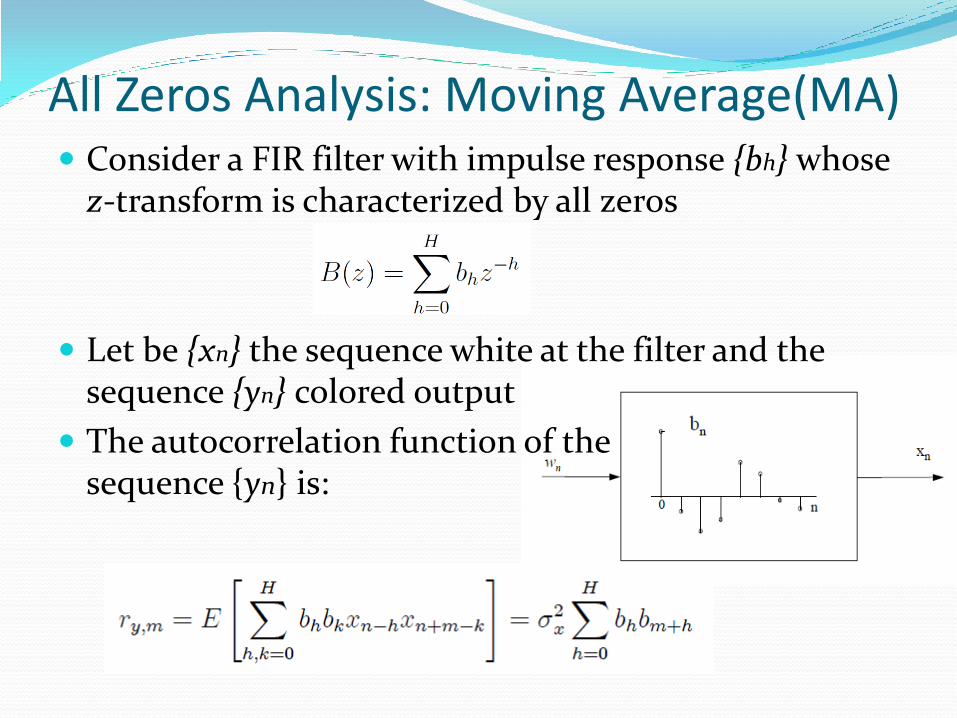
All Zeros Analysis: Moving Average(MA) Consider a FIR filter with impulse response {bh} whose
z-transform is characterized by all zeros
Let be {xn} the sequence white at the filter and the sequence {yn} colored output
The autocorrelation function of the sequence {yn} is:
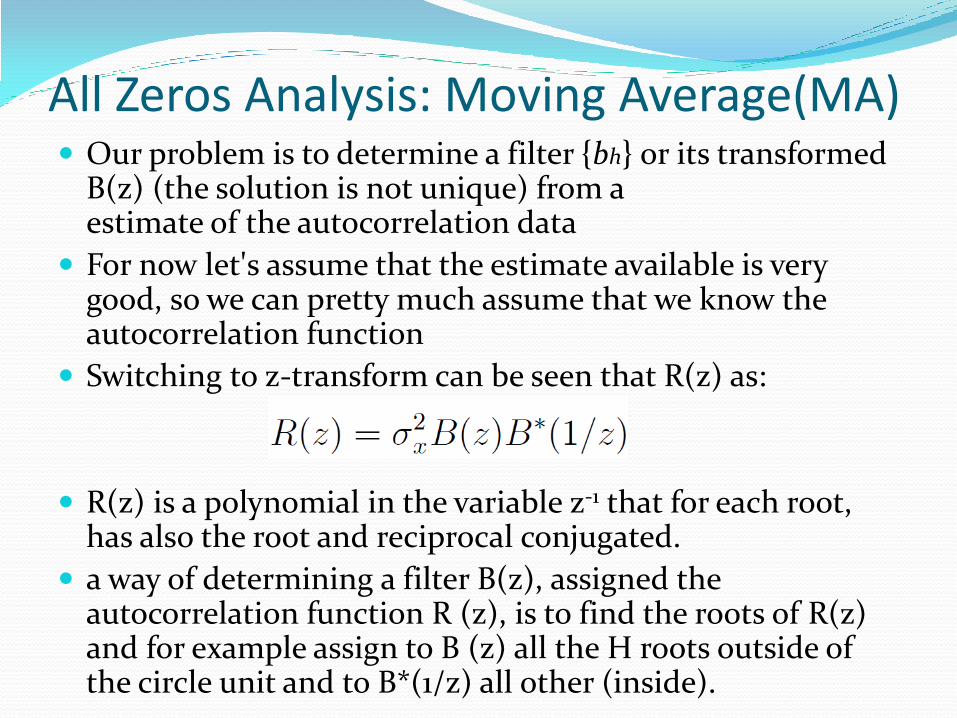
Our problem is to determine a filter {bh} or its transformed B(z) (the solution is not unique) from a estimate of the autocorrelation data
For now let's assume that the estimate available is very good, so we can pretty much assume that we know the autocorrelation function
Switching to z-transform can be seen that R(z) as:
R(z) is a polynomial in the variable z-1 that for each root, has also the root and reciprocal conjugated.
a way of determining a filter B(z), assigned the autocorrelation function R (z), is to find the roots of R(z) and for example assign to B (z) all the H roots outside of the circle unit and to B*(1/z) all other (inside).
All Zeros Analysis: Moving Average(MA)

All Zeros Analysis: Moving Average(MA) following the strategy of the previous slide, B*(1/z) is
minimum phase, otherwise we can choose B*(1/z) at maximum phase or mixed phase, in different ways 2H
Note that it is not enough that R (z) is a any polynomial for identifying a filter B(z).
In fact, there would be reciprocal pairs of zeros but it could also have simple zeros on unit circle, in which case it would not be possible to find the B(z) because you can not associate a mutual positioned root
But in this case, the symmetrical polynomial R(z) would not represent an autocorrelation function
the values of the R(z) on the unit circle, contain changes sign when passing through the zeros and then negative values
while instead a power spectrum, Transform Fourier autocorrelation function, is always positive
Minimum Phase
Maximum Phase
Mixed Phase
Truncation of the autocorrelation We have an autocorrelation function equal to zero for m>H It is always possible to find 2H filters of length H + 1 that
powered by white sequences return in the output the autocorrelation
However, there are only estimates of the autocorrelation function: if the estimate is made with the correlation of the sequence padded with zeros, then its Fourier transform, (the periodogram) is always positive.
in this case, the length of the filter is excessive because, due to the dispersion of the estimate, the samples of the autocorrelation estimated will never be zero
If we want to limit the length of the filter to H, it should be squash to O, the autocorrelation function in H samples, windowing it so that the spectrum remains positive, and then multiplying it by a window which in practice is always the triangular
Truncation of the autocorrelation In conclusion, to make a all zeros parametric
estimation, it is necessary to window the autocorrelation function with a triangular window of length 2H;
Incising H greater will be the resolution of the spectral parameter estimation
In essence, it is seen that this technique of spectral estimation coincides with that of the smoothing periodogram

Analysis All Poles(AR) Preliminary Observations
This technique of spectral estimation is very important for many reasons.
it should be noted that the IIR filters having unlimited impulse response, they can produce spectra of large spectral resolution with a limited number of parameters
lend themselves to the description of phenomena that have a long coherence time, i.e. where the process uncurreled very slowly.
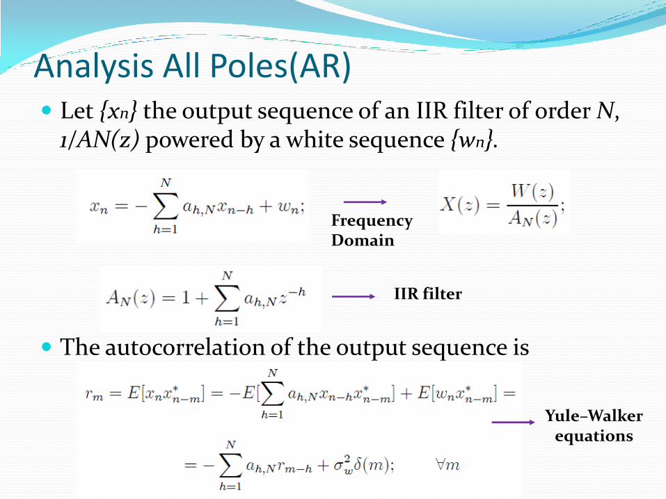
Analysis All Poles(AR) Let {xn} the output sequence of an IIR filter of order N,
1/AN(z) powered by a white sequence {wn}.
The autocorrelation of the output sequence is
Frequency Domain
IIR filter
Yule–Walker equations

Yule–Walker equations Yule Walker equations can be obtained in the matrix form
indicating the following vectors with the symbols:
multiplying on the left by ξN and considering the expected
value, whereas E[xN wn] = O we obtain

Yule–Walker equations The matrix of the coefficients of the YW equations is a Toeplitz matrix;
It is symmetric (or Hermitian, for complex sequences) and all the elements belonging to the same diagonal or subdiagonale are equal to each other.
The matrix is characterized by N numbers.
Rewriting in matrix form, the equations of Yule Walker is obtained
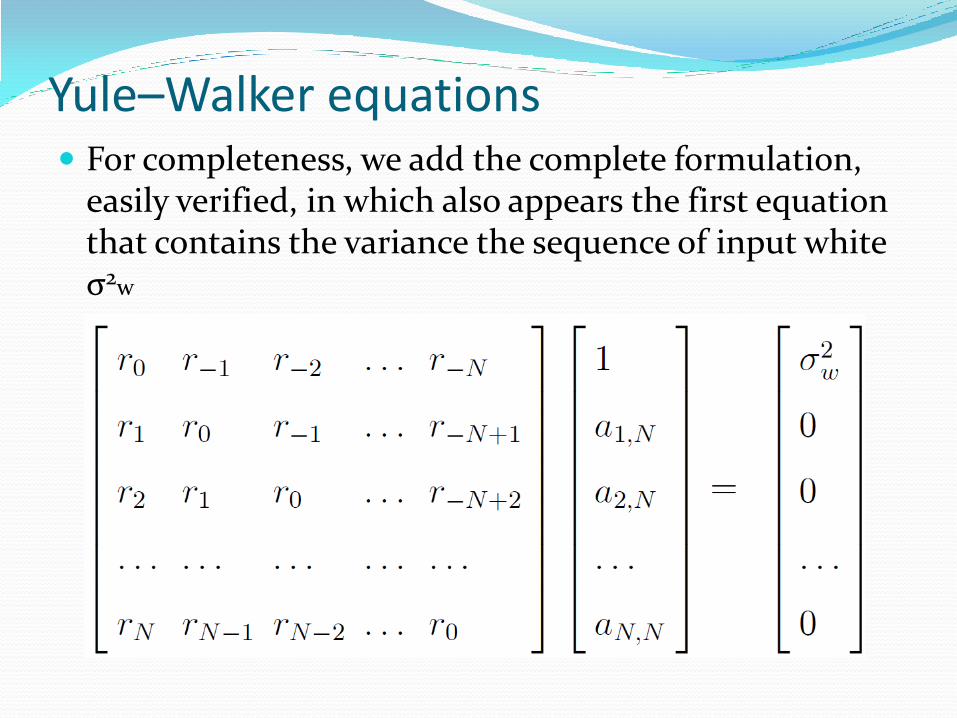
Yule–Walker equations For completeness, we add the complete formulation,
easily verified, in which also appears the first equation that contains the variance the sequence of input white σ2w
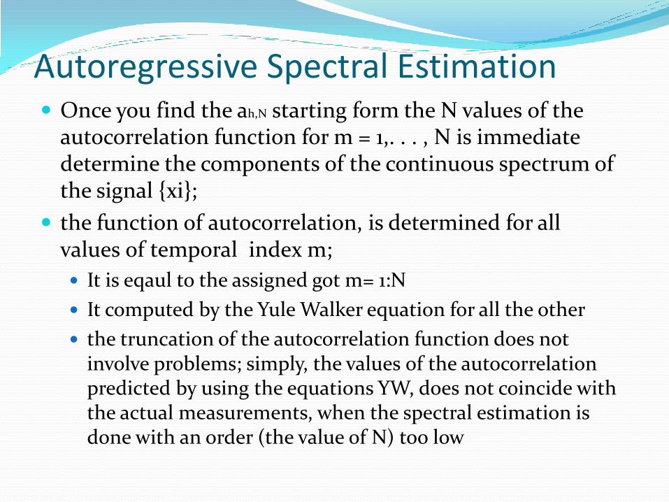
Autoregressive Spectral Estimation Once you find the ah,N starting form the N values of the
autocorrelation function for m = 1,. . . , N is immediate determine the components of the continuous spectrum of the signal {xi};
the function of autocorrelation, is determined for all values of temporal index m;
It is eqaul to the assigned got m= 1:N
It computed by the Yule Walker equation for all the other
the truncation of the autocorrelation function does not involve problems; simply, the values of the autocorrelation predicted by using the equations YW, does not coincide with the actual measurements, when the spectral estimation is done with an order (the value of N) too low
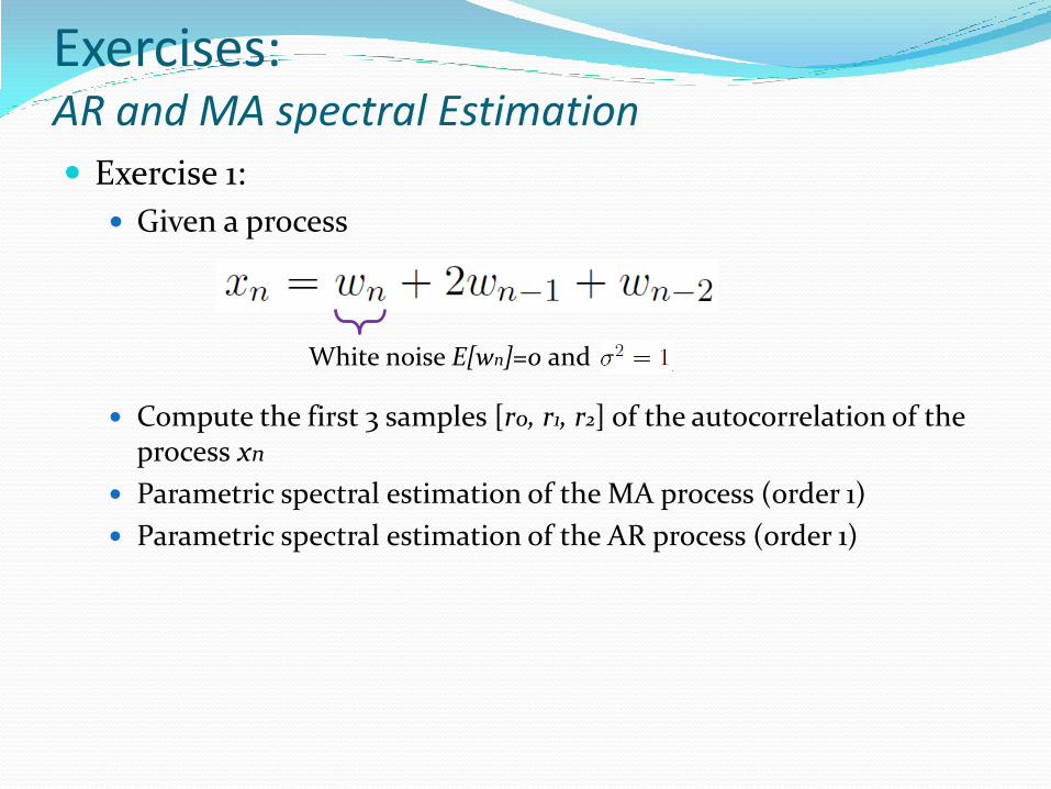
Exercises: AR and MA spectral Estimation
Exercise 1:
Given a process
Compute the first 3 samples [r0, r1, r2] of the autocorrelation of the
process xn
Parametric spectral estimation of the MA process (order 1)
Parametric spectral estimation of the AR process (order 1)
White noise E[wn]=0 and
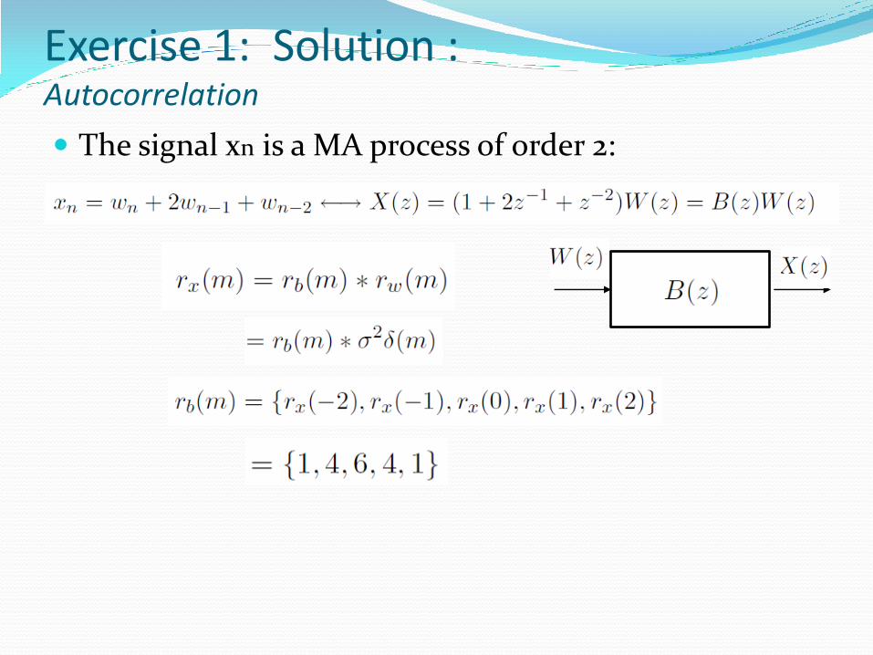
The signal xn is a MA process of order 2:
Exercise 1: Solution : Autocorrelation
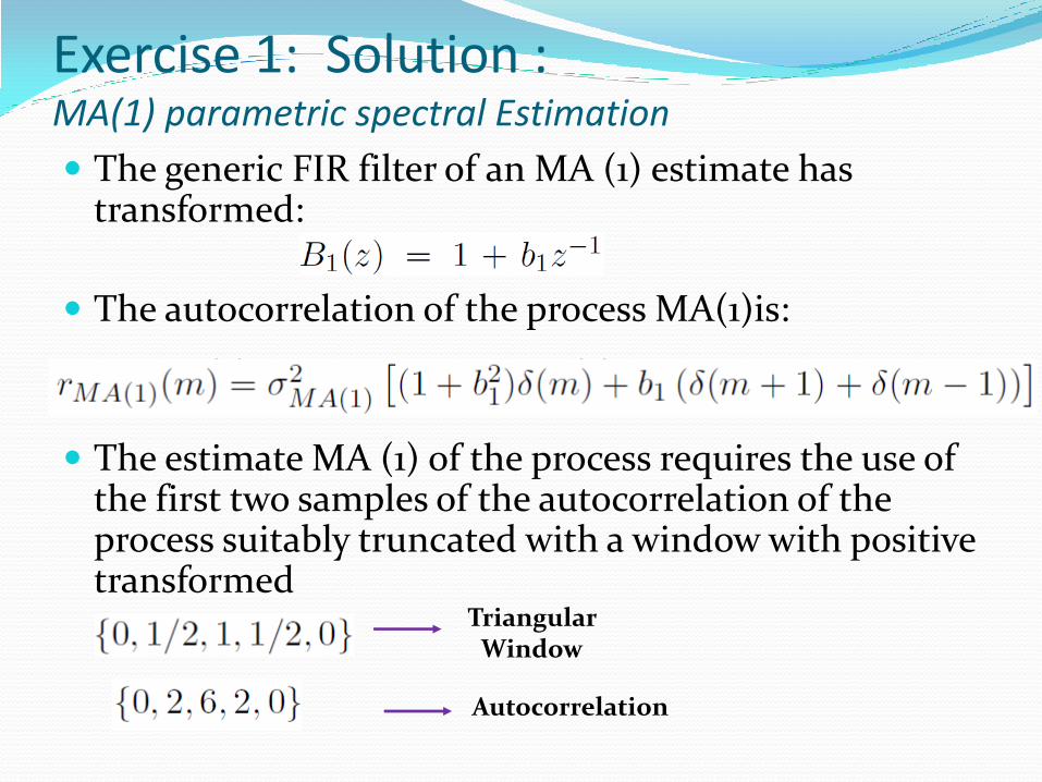
The generic FIR filter of an MA (1) estimate has transformed:
The autocorrelation of the process MA(1)is:
The estimate MA (1) of the process requires the use of the first two samples of the autocorrelation of the process suitably truncated with a window with positive transformed
Exercise 1: Solution : MA(1) parametric spectral Estimation
Triangular Window
Autocorrelation
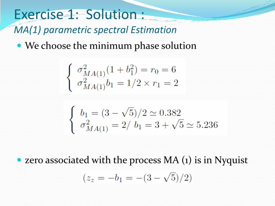
We choose the minimum phase solution
zero associated with the process MA (1) is in Nyquist
Exercise 1: Solution : MA(1) parametric spectral Estimation
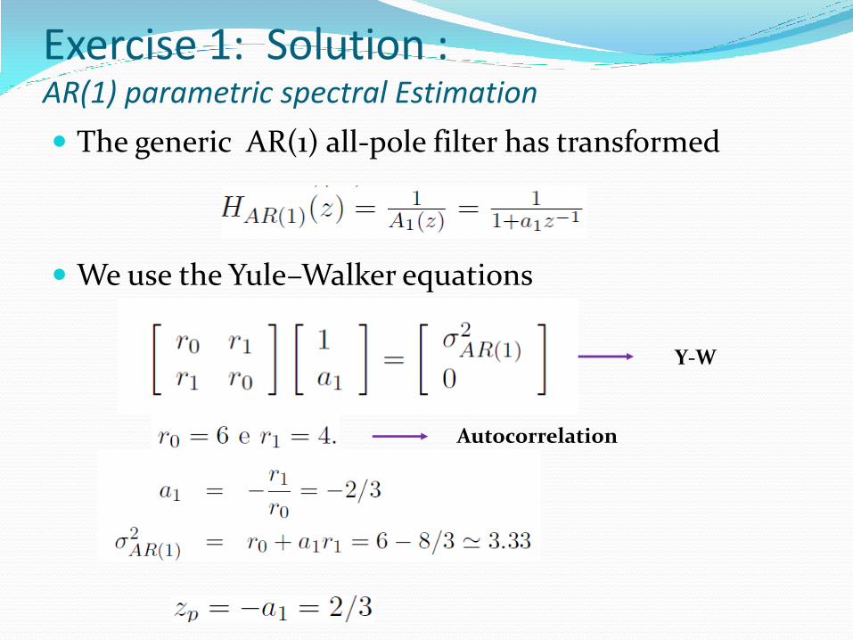
The generic AR(1) all-pole filter has transformed
We use the Yule–Walker equations
Exercise 1: Solution : AR(1) parametric spectral Estimation
Y-W
Autocorrelation
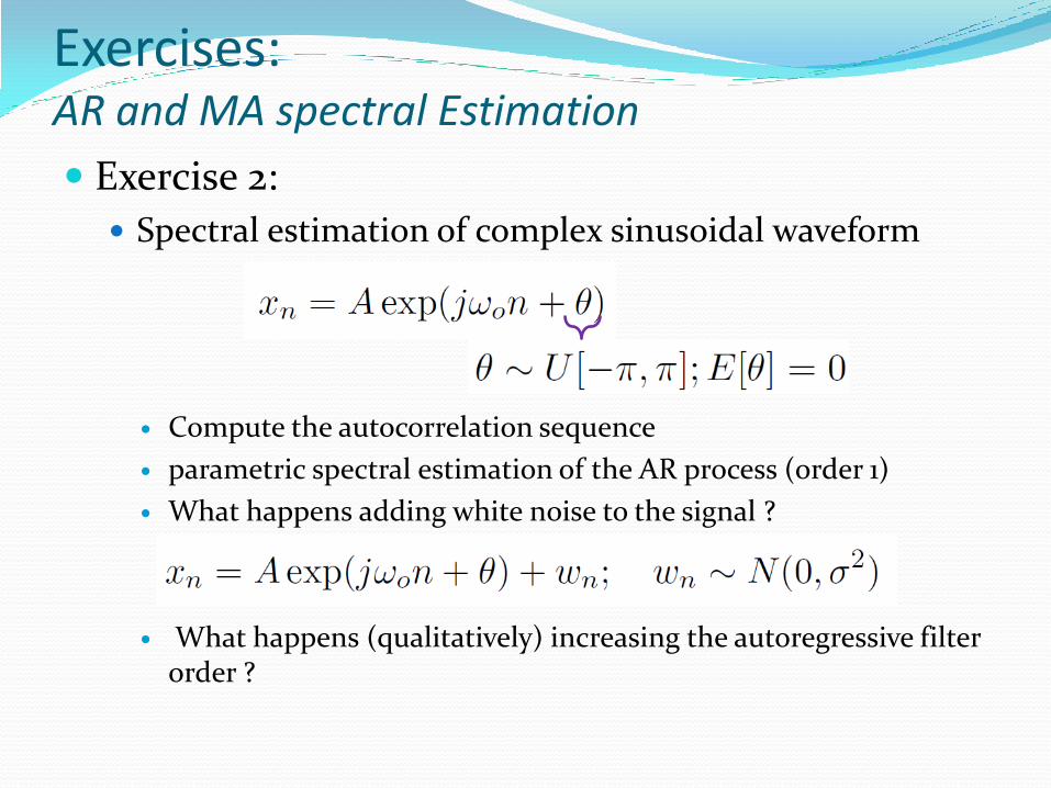
Exercise 2:
Spectral estimation of complex sinusoidal waveform
Compute the autocorrelation sequence
parametric spectral estimation of the AR process (order 1)
What happens adding white noise to the signal ?
What happens (qualitatively) increasing the autoregressive filter order ?
Exercises: AR and MA spectral Estimation
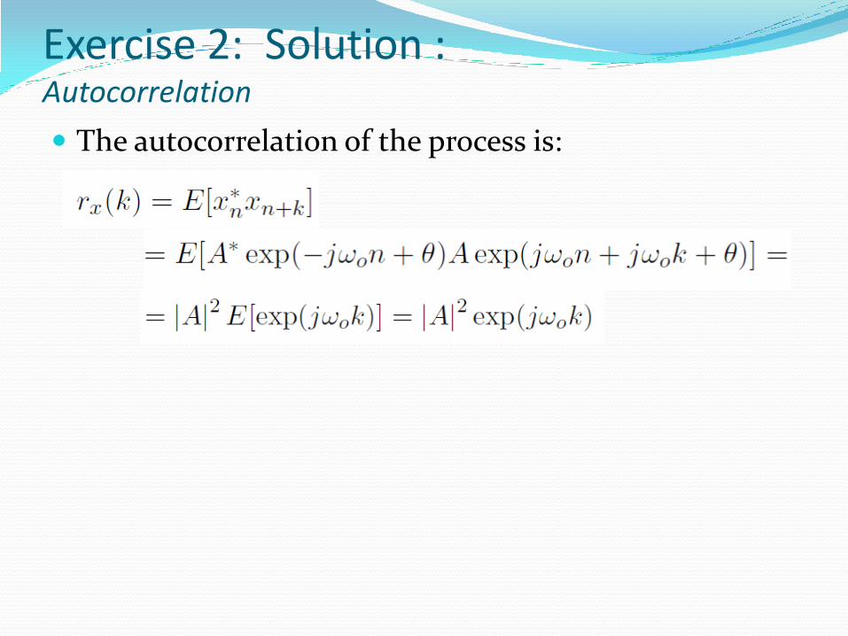
The autocorrelation of the process is:
Exercise 2: Solution : Autocorrelation
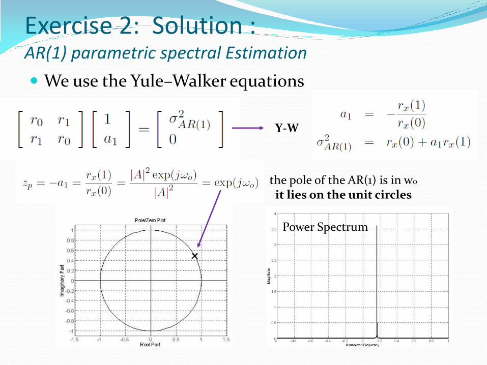
We use the Yule–Walker equations
Exercise 2: Solution : AR(1) parametric spectral Estimation
Y-W
the pole of the AR(1) is in wo it lies on the unit circles
Power Spectrum

Autocorrelation
Using the Y-W equation
Exercise 2: Solution What happens adding white noise to the signal ?
In the presence of a white noise the frequency of the pole model of the AR (1) remains unchanged
The radial position is changed. The pole is closer to the origin of a quantity proportional to the signal to noise ratio

Exercise 2: Solution What happens adding white noise to the signal ?
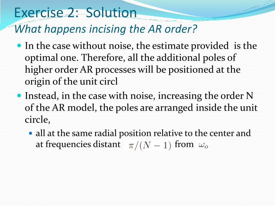
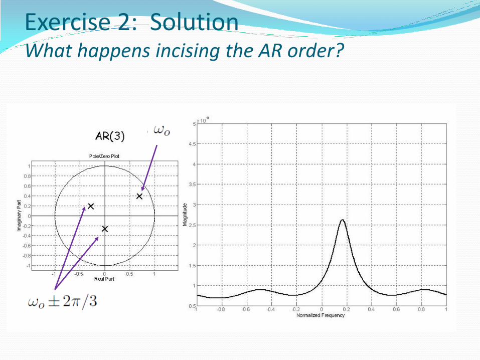
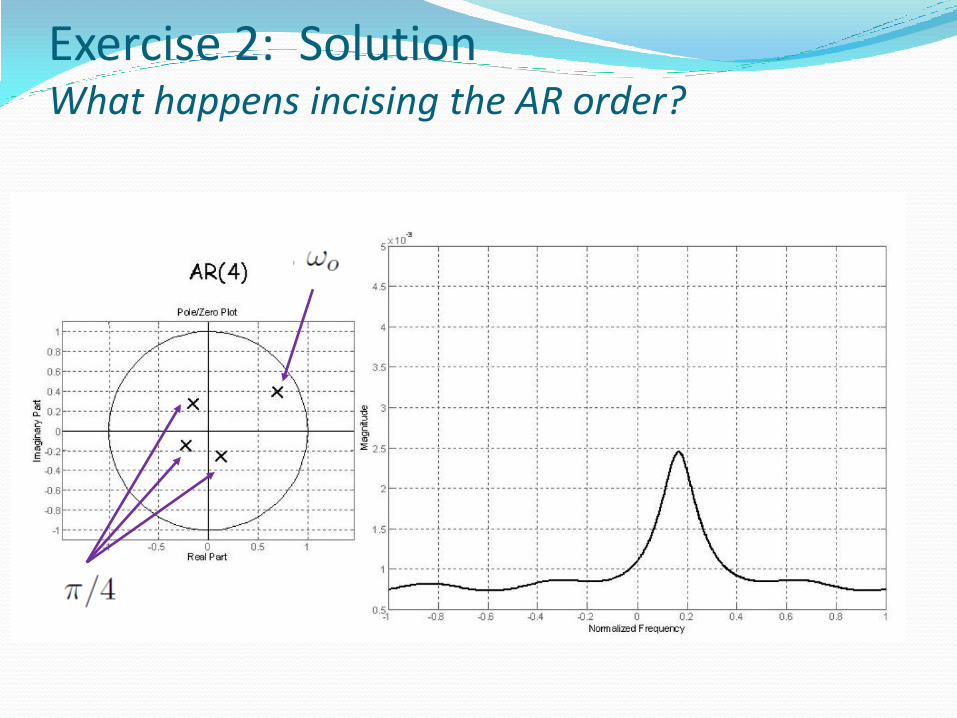
In the case without noise, the estimate provided is the optimal one. Therefore, all the additional poles of higher order AR processes will be positioned at the origin of the unit circl
Instead, in the case with noise, increasing the order N of the AR model, the poles are arranged inside the unit circle,
all at the same radial position relative to the center and at frequencies distant from
Exercise 2: Solution What happens incising the AR order?

Exercise 2: Solution What happens incising the AR order?
Exercise 2: Solution What happens incising the AR order?
Exercise 2: Solution What happens incising the AR order?

Autoregressive Model Hint:
The parametric of model-based methods of spectral estimation assume that the signal satisfies a generating model with known functional form, and then proceed in estimating the parameters in the assumed model Power Spectral Density
Matlab Examples: Autoregressive Model
Autoregressive Model
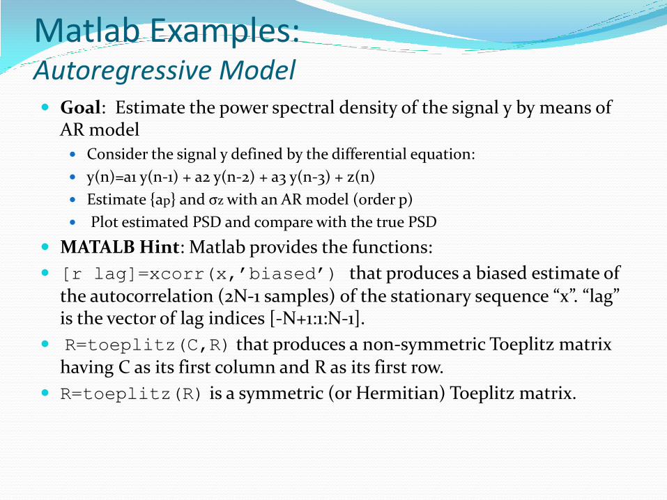
Goal: Estimate the power spectral density of the signal y by means of AR model
Consider the signal y defined by the differential equation:
y(n)=a1 y(n-1) + a2 y(n-2) + a3 y(n-3) + z(n)
Estimate {ap} and σz with an AR model (order p)
Plot estimated PSD and compare with the true PSD
MATALB Hint: Matlab provides the functions:
[r lag]=xcorr(x,’biased’) that produces a biased estimate of the autocorrelation (2N-1 samples) of the stationary sequence “x”. “lag” is the vector of lag indices [-N+1:1:N-1].
R=toeplitz(C,R) that produces a non-symmetric Toeplitz matrix having C as its first column and R as its first row.
R=toeplitz(R) is a symmetric (or Hermitian) Toeplitz matrix.
Matlab Examples: Autoregressive Model

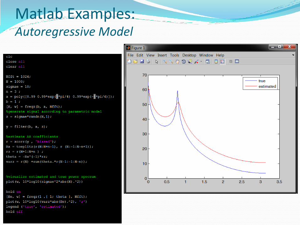
Pseudocode: Consider the signal y defined by the differential equation: y(n)=a1 y(n-1) + a2 y(n-2) + a3 y(n-3) + z(n)
sigmae = 10;
a = poly([0.99 0.99*exp(j*pi/4) 0.99*exp(-j*pi/4)])
b = 1 ;
z = sigmae*randn(N,1);
y = filter(b, a, z); Estimate {ap} and σz with an AR model (order p)
n=3;
r = xcorr(y , 'biased');
Rx = toeplitz(r(N:N+n-1), r (N:-1:N-n+1));
rz = r(N+1:N+n ) ;
theta = -Rx^(-1)*rz;
varz = r(N) +sum(theta.*r(N-1:-1:N-n));
Plot estimated PSD and compare with the true PSD
Matlab Examples: Autoregressive Model
Matlab Examples: Autoregressive Model
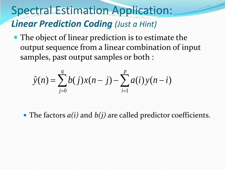
Spectral Estimation Application: Linear Prediction Coding (Just a Hint)
The object of linear prediction is to estimate the output sequence from a linear combination of input samples, past output samples or both :
The factors a(i) and b(j) are called predictor coefficients.
p
i
q
j
inyiajnxjbny10
)()()()()(ˆ
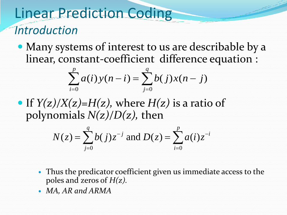
Linear Prediction Coding Introduction
Many systems of interest to us are describable by a linear, constant-coefficient difference equation :
If Y(z)/X(z)=H(z), where H(z) is a ratio of polynomials N(z)/D(z), then
Thus the predicator coefficient given us immediate access to the
poles and zeros of H(z).
MA, AR and ARMA
q
j
p
i
jnxjbinyia00
)()()()(
p
i
iq
j
j ziazDzjbzN00
)()( and )()(
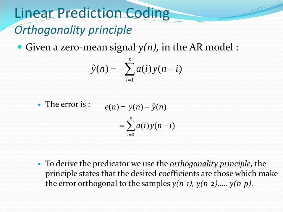
Given a zero-mean signal y(n), in the AR model :
The error is :
To derive the predicator we use the orthogonality principle, the principle states that the desired coefficients are those which make the error orthogonal to the samples y(n-1), y(n-2),…, y(n-p).
p
i
inyiany1
)()()(ˆ
p
i
inyia
nynyne
0
)()(
)(ˆ)()(
Linear Prediction Coding Orthogonality principle

Thus we require that
Or,
Interchanging the operation of averaging and summing, and representing < > by summing over n, we have
The required predicators are found by solving these equations.
p..., 2, 1,jfor 0)()( nejny
p1,...,j ,0)()()(0
n
p
i
jnyinyia
Linear Prediction Coding Orthogonality principle
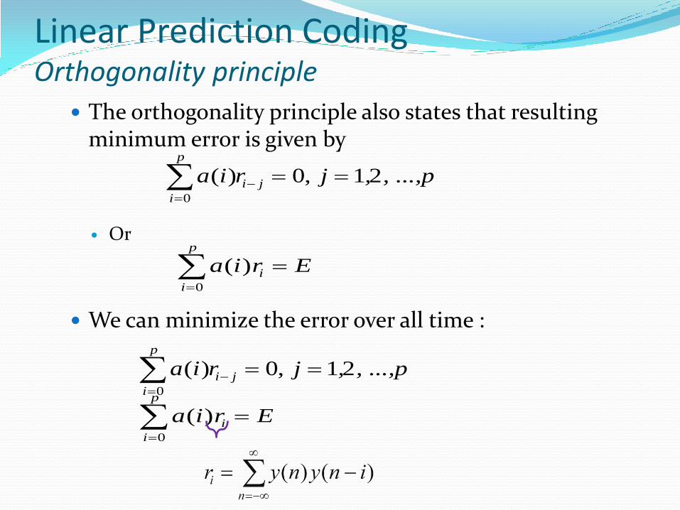
The orthogonality principle also states that resulting minimum error is given by
Or
We can minimize the error over all time :
, ...,p,jria ji
p
i
21 ,0)(0
Eriap
i
i 0
)(
, ...,p,jria ji
p
i
21 ,0)(0
Eriap
i
i 0
)(
Linear Prediction Coding Orthogonality principle