1

FULL TITLE

A comparison of logistic regression and classification tree analysis for behavioural case

linkage

SHORT TITLE

Behavioural linking using regression and classification tree analysis

Tonkin, M., Woodhams, J., Bull, R., Bond, J. W., & Santtila, P.

Keywords

Case linkage; comparative case analysis; regression; classification trees

2

Abstract

Much previous research on behavioural case linkage has used binary logistic regression to

build predictive models that can discriminate between linked and unlinked offences.

However, classification tree analysis has recently been proposed as a potential alternative due

to its ability to build user-friendly and transparent predictive models. Building on previous

research, the current study compares the relative ability of logistic regression analysis and

classification tree analysis to construct predictive models for the purposes of case linkage.

Two samples are utilised in this study: a sample of 376 serial car thefts committed in the

United Kingdom (UK) and a sample of 160 serial residential burglaries committed in Finland.

In both datasets logistic regression and classification tree models achieve comparable levels

of discrimination accuracy, but the classification tree models demonstrate problems in terms

of reliability or usability that the logistic regression models do not. These findings suggest

that future research is needed before classification tree analysis can be considered a viable

alternative to logistic regression in behavioural case linkage.

3

A comparison of logistic regression and classification tree analysis for behavioural case

linkage

Behavioural case linkage uses similarity in Modus Operandi (MO) behaviour and

geographical proximity to identify groups of crimes that were committed by the same

offender (referred to as linked crime series). The process of identifying groups of so-called

“linked offences” is of potential benefit to the police and other investigative agencies for

several reasons. First, it allows the collation and pooling of information from several different

crime scenes, which potentially increases the quantity and quality of evidence against an

offender and, therefore, the likelihood of a successful prosecution (Grubin, Kelly, &

Brunsdon, 2001). Second, the process of drawing together multiple investigations can help

the police to work in a more streamlined and efficient manner, as it allows them to conduct

one-overarching investigation that avoids the unnecessary duplication of roles and

responsibilities than can occur when multiple crimes are investigated separately (Woodhams,

Hollin, & Bull, 2007). Academic and practical interest in behavioural case linkage has,

therefore, grown significantly in recent years, with a number of publications (e.g., Bennell &

Canter, 2002; Santtila, Junkkila, & Sandnabba, 2005; Tonkin, Grant, & Bond, 2008) and

evidence that linkage is becoming increasingly used during police investigations and court

proceedings (e.g., Charron & Woodhams, 2010; Hazelwood & Warren, 2003; Labuschagne,

2012).

In terms of the academic interest in behavioural case linkage, several different

methodological approaches have been developed to test the underlying principles of case

linkage. However, the most commonly used methodology was developed by Dr. Craig

Bennell (e.g., Bennell & Canter, 2002). This methodology uses binary logistic regression and

Receiver Operating Characteristic (ROC) analyses to test the ability of offender behaviour to

4

distinguish between linked and unlinked offences. Statistically significant regression models

and relatively large Area Under the Curve (AUC) values are thought to indicate the potential

for offender behaviour to facilitate case linkage in practice1.

Using this and other methodologies, a number of studies have demonstrated that

certain types of offender behaviour can be used to distinguish between linked and unlinked

offences to a statistically significant extent. This evidence spans a variety of different crime

types, including burglary, robbery, car theft, sexual assault, homicide, and arson (e.g.,

Bennell, Jones, & Melnyk, 2009; Melnyk, Bennell, Gauthier, & Gauthier, 2010; Santtila,

Fritzon, & Tamelander, 2004; Tonkin et al., 2008; Woodhams & Toye, 2007). For example,

Woodhams and Toye (2007) showed that a logistic regression model combining three types

of offender behaviour (control, planning, and intercrime distance2) was able to distinguish

between linked and unlinked commercial robberies with a high degree of accuracy (AUC =

0.95; Swets, 1988). This level of accuracy suggests that behavioural case linkage may be a

viable procedure for the police to use. Also, these findings highlight specific offender

behaviours that can be used to guide case linkage.

But, despite the growing body of work on case linkage and the promising initial

findings, this literature is still in its infancy. For example, research is only just beginning to

explore the many methodological issues that surround the empirical testing of case linkage

(e.g., Melnyk et al., 2010; Tonkin, Santtila, & Bull, 2011; Woodhams, Grant, & Price, 2007).

One recent methodological issue that has been explored is the use of classification tree

analysis instead of logistic regression to produce statistical models that can discriminate

between linked and unlinked offences (Bennell, Woodhams, & Beauregard, in preparation).

Binary logistic regression has been used in several previous studies of case linkage

(e.g., Bennell & Canter, 2002; Woodhams & Toye, 2007) and has advantages over other

statistical procedures, such as discriminant function analysis, because it can cope with a

5

wider variety of variables and is more resistant to violations of normality and homogeneity

that are common in this area of research (Kinnear & Gray, 2009). However, the limitations of

logistic regression have been recognised within another area of forensic psychology — the

risk assessment literature — for over a decade (e.g., Steadman et al., 2000) and have recently

been applied to the literature on behavioural case linkage (Bennell et al., in preparation). To

illustrate the relative advantages of classification tree analysis over logistic regression, it is

useful to consider how these procedures might be utilised in practice to facilitate the linking

of crime.

In terms of logistic regression, the outcome of a successful analysis is a formula that

can be used to predict whether crimes are linked or not. Depending on which types of

offender behaviour emerge as statistically significant in the regression analysis, the formula

combines the relevant behavioural information into a predicted probability value that

indicates the likelihood of two crimes being committed by the same person3. This value

ranges from 0 (indicating that the two crimes are unlikely to be linked) to 1.00 (indicating

that the two crimes are likely to be linked). An automated tool could be designed to perform

these calculations, thus allowing an analyst to calculate a predicted probability value for all

pairwise comparisons in a given dataset of crimes (e.g., the probability of crime 1 and crime

2 being linked, the probability of crime 1 and crime 3 being linked, and so on). The

probability values could then be arranged in order from highest to lowest, thereby providing

the analyst with a prioritised list of potentially linked crimes. This may help to reduce

cognitive load and avoid linkage blindness during the early stages of case linkage.

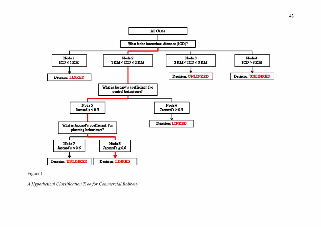
In contrast, classification tree analysis provides the analyst with a structured set of

questions that can be used to decide whether two crimes are linked or not (see the

hypothetical example in Figure 1). These questions are organised hierarchically such that the

first question is asked of all cases but subsequent questions can differ depending on the

6

preceding answer (Gardner, Lidz, Mulvey, & Shaw, 1996; Liu, Yang, Ramsay, Li, & Coid,

2011). This set of questions is followed until the analyst reaches a decision regarding linkage.

As an example, consider a situation where an analyst is presented with two commercial

robberies that are 1.50 kilometres apart and have been assessed as having a Jaccard’s

coefficient of 0.43 for control behaviours and 0.82 for planning behaviours (Jaccard’s

coefficient is a measure of behavioural similarity that ranges from 0, indicating no similarity,

to 1.00, indicating complete similarity). To determine whether these two crimes are linked,

the analyst would start at the top of the tree with the question ‘What is the intercrime

distance?’ Given an intercrime distance of 1.50 kilometres, the analyst would determine that

the case falls within node 2, which subsequently leads to the next question in the hierarchy

(‘What is the size of the Jaccard’s coefficient for control behaviours?’). In this example the

crime pair has a coefficient of 0.43 for control behaviours, which indicates that the case falls

within node 5, therefore, leading to the final question (‘What is the size of the Jaccard’s

coefficient for planning behaviours?’). A coefficient of 0.82 for planning behaviours places

the crime pair in node 8, thereby leading the analyst to conclude that these two robbery

crimes are linked. The path that the analyst took through the decision tree in this example is

highlighted in red on Figure 1.

Classification tree analysis, therefore, provides the analyst with a structured decision-

making process that indicates which types of offender behaviour should be used to link crime

and how these behaviours can be used to do so. Importantly, this process does not require the

analyst to perform complex mathematical calculations when linking crime (Rosenfeld &

Lewis, 2005); they simply need to calculate the relevant similarity coefficients and to follow

the hierarchy of questions from start to finish (all of which could be automated). Logistic

regression, however, requires the analyst to perform several analytical steps (see the Method

section). Although this process could be automated, the analyst would still need to understand

7

how the logistic regression function has arrived at a particular decision so that they can

explain their decision-making processes to investigating officers and/or the courts (which

they often have to do). This is inherently difficult for a decision that is based on a

mathematical equation, which can be difficult to break down into its constituent parts.

Decisions that are based on a classification tree, however, are relatively easy to understand

and explain because they are depicted visually (Gardner et al., 1996). In the hypothetical

crime pair above, for example, it is clear from Figure 1 which behaviours were used to

determine whether the crimes were linked and how these behaviours were used to guide the

analyst through the hierarchy of questions. Arguably, this may increase the likelihood of tree-

based linkage models becoming accepted in practice by crime analysts compared to

regression-based models (Bennell et al., in preparation; Woodhams, Bennell, & Beauregard,

2011).

A further advantage is that classification tree analysis does not assume that the same

predictor variables apply to every case, whereas logistic regression does (Steadman et al.,

2000). To illustrate this point, consider the crime pair discussed above and highlighted in

Figure 1. In this example the analyst used the intercrime distance, control and planning

behaviours to reach a decision that the two crimes were linked. If, however, another crime

pair were considered that had an intercrime distance of 0.53 kilometres the control and

planning behaviours would not be needed to reach a decision because the crime pair would

fall into node 1, thereby leading to the crimes being linked (see Figure 1). This situation

would not arise, though, with a logistic regression model because the same logistic function

(and, therefore, the same offender behaviours) would be applied to both cases to determine

linkage (Monahan et al., 2001). Arguably, this feature would make classification tree

approaches more appealing to practitioners who tend to emphasise the heterogeneity in

offending behaviour (Steadman et al., 2000). Furthermore, when one inspects the case

8

linkage literature, there is evidence to suggest that behavioural consistency may be expressed

differentially from one offender to the next, which would make the “one size fits all”

approach of logistic regression inappropriate (e.g., Grubin et al., 2001; Woodhams, 2008).

For example, Grubin et al. (2001) analysed the behavioural consistency displayed by serial

sex offenders in the United Kingdom (UK) and Canada. They found that behavioural

consistency was evident in the crime scene behaviour of their sample, but the nature of this

consistency was not the same for all offenders. That is, some offenders displayed consistency

in their control behaviours, while others displayed consistency in their escape behaviours, and

some were consistent in their sexual behaviours. In short, classification tree analysis may be

more consistent with the empirical reality of offender behavioural consistency, thereby

making it more suitable for use in practice than logistic regression (Bennell et al., in

preparation; Woodhams et al., 2011).

However, researchers have also noted some potential disadvantages of using

classification trees relative to logistic regression. In particular, several studies have observed

a tendency for the predictive models produced using classification tree analysis to be less

robust when applied to new data than those produced using logistic regression (e.g.,

Rosenfeld & Lewis, 2005; Thomas et al., 2005). This phenomenon has been referred to as

“shrinkage” or “over-fitting of the data” (e.g., Thomas et al., 2005). It occurs when complex

models are produced by combining multiple predictive factors, which fit the training sample

well but fail to generalise to new datasets (Liu et al., 2011). It, therefore, seems that one of

the proposed advantages of classification tree analysis, where different predictive factors are

used for different cases, may sometimes lead to an overly-complex model that is not very

robust. This could be a substantial problem where research is trying to build models that can

be applied in future practical situations, as is the case in the case linkage literature.

9

To investigate the relative merits of classification tree analysis and logistic regression

in a case linkage context, Bennell et al. (in preparation) recently analysed samples of

residential burglary, commercial robbery, and rape. They found that an iterative approach to

building classification trees (Monahan et al., 2001; Steadman et al., 2000) was able to

discriminate between linked and unlinked offences at a level that was comparable to that

using logistic regression analysis. For the sample of adult stranger rapes they studied, an

AUC of 0.99 was achieved using classification tree analysis, which compared to an AUC of

0.98 using logistic regression. For the sample of commercial robberies, classification tree

analysis achieved an AUC of 0.84, compared to an AUC of 0.90 using logistic regression.

For the sample of residential burglaries, classification tree analysis achieved an AUC of 0.87,

which compared to an AUC of 0.91 using logistic regression. While the logistic regression

AUCs were marginally larger than the tree-based models with the samples of robbery and

burglary in Bennell et al.’s (in preparation) study, the overlapping confidence intervals

indicated that these AUC values were not significantly different (Melnyk et al., 2010). The

authors, therefore, concluded that classification tree analysis may be a useful alternative to

logistic regression when it comes to building models that can assist crime analysts in the case

linkage task.

The comparable performance of logistic regression and tree-based models in Bennell

et al. (in preparation) are similar to those that have been observed in the wider medical and

forensic literatures. For example, a number of studies within the risk assessment literature

have shown that various main effects and tree-based regression approaches, as well as a

neural networks model, produce largely comparable levels of accuracy when predicting

violent reoffending (see Liu et al., 2011, for a review).

However, the level of shrinkage that occurred when Bennell and colleagues applied

the classification trees from the training sample to the test sample in their study is currently

10

unclear. This is an important piece of information for evaluating model performance, as

practitioners must be able to report the expected level of error that is involved in their linkage

predictions. For example, one of the key components of Rule 702 of the Federal Rules of

Evidence, which guides the acceptance of expert evidence in American courts of law, is that

any theory or technique being presented in court must have a known or potential error rate.

Thus, it is important that statistical approaches to case linkage are shown to achieve relatively

stable levels of discrimination accuracy from one sample to the next; otherwise it will be

difficult to give an accurate estimate of the error rate. Furthermore, findings from the risk

assessment literature have demonstrated significant shrinkage in the discrimination accuracy

of classification trees when they have been applied to training and test samples separately

(e.g., Liu et al., 2011; Rosenfeld & Lewis, 2005; Thomas et al., 2005). The extent to which

classification tree analysis is able to produce robust and generalisable predictive models for

the purposes of linking crime cannot, therefore, be fully evaluated unless the level of

shrinkage is explicitly reported.

It is also important that we do not assume that the findings from one study will

necessarily replicate with other crime types and in different areas. For example, Tonkin et al.

(2011) recently demonstrated that case linkage findings developed in one country (the UK)

can be substantially different when applied to another county (Finland). The current study,

therefore, compared the ability of logistic regression analysis and classification tree analysis

to build predictive models that can distinguish between linked and unlinked car thefts that

were committed in the UK and between linked and unlinked residential burglaries that were

committed in Finland. Classification tree analysis has never been applied to car theft data

before nor has it been applied to residential burglaries outside of the UK.

Method

11

Samples

Residential burglary data. The residential burglary data consisted of 160 residential

burglaries committed by 80 serial burglars in the Greater Helsinki region of Finland4 between

1990 and 2001. These data were originally collected as part of a previous project (Laukkanen,

Santtila, Jern, & Sandnabba, 2008; Santtila, Ritvanen, & Mokros, 2004). Two crimes per

offender were randomly selected from the total number of offences that they had committed

during this time period. Previous research has considered it necessary to select a constant

number of offences per offender so as to prevent highly prolific offenders with unusually

consistent or inconsistent offence behaviour having an undue influence on the findings

(Bennell, 2002).

For each burglary a range of behavioural data were recorded, including the location of

the crime (stored as an x, y coordinate), the type of property burgled, the method of entry, the

search behaviour, and the type and cost of property stolen (see Tonkin et al., 2011, for further

details). Apart from the location information, the data were stored in a binary format (1 =

present in the crime; 0 = absent). The use of binary data is consistent with previous research

on behavioural case linkage (e.g., Bennell & Canter, 2002) and is justified by findings

suggesting that more complex coding schemes are unreliable with police data (Canter &

Heritage, 1990).

Car theft data. The car theft data consisted of 376 vehicle theft crimes committed by

188 serial car thieves in Northamptonshire, UK, between January 2004 and May 2007. Two

crimes per offender were randomly selected from the total number of offences that they had

committed during this time period (Bennell, 2002). These data were collected as part of a

previous project (Tonkin, 2007), but were only used for preliminary analyses in that work.

Thus, analyses using these data have not been previously published.

12

For each car theft a range of behavioural data were recorded, including the location of

the crime (an x, y coordinate), the type of car that was stolen, the age of the vehicle, the time

and day of the week the vehicle was stolen, how the vehicle was entered and started, and the

physical state in which the vehicle was recovered (see Tonkin et al., 2008, for further details).

Apart from the location information, the data were stored in a binary format (Canter &

Heritage, 1990).

Procedure

First, a number of behavioural domains were created for each dataset. Behavioural

domains contain clusters of individual offender behaviours that serve either a similar function

during the offence, that occur at a similar stage of the offence, or that represent one ‘type’ of

offender behaviour (Tonkin et al., 2011). For the burglary data, six behavioural domains were

created, each containing a cluster of individual behavioural variables: 1) Target

Characteristics (containing 12 behavioural variables, e.g., the type of property burgled); 2)

Entry Behaviours (containing 20 variables, e.g., the point and method of entry); 3) Internal

Behaviours (containing 21 variables, e.g., search behaviour); 4) Property Stolen (containing

31 variables, e.g., cash, keys etc.); 5) The Intercrime Distance (the geographical distance in

kilometres between two offence locations); 6) A Combined behavioural domain, which

included all behaviours in the target, entry, internal, and property domains (82 variables).

These domains were derived from previous case linkage studies of burglary and the

behaviours were placed into domains according to their placement in previous research (e.g.,

Bennell, 2002; Markson, Woodhams, & Bond, 2010; Tonkin et al., 2011).

For the car theft data, five behavioural domains were created: 1) Target Selection

Choices (containing 27 individual behavioural variables, e.g., the type and age of the vehicle

stolen, and the time of day and day of the week of the theft); 2) Target Acquisition Behaviour

13

(containing nine variables, e.g., the method and point of entry to the vehicle); 3) Disposal

Behaviour (containing eight variables, e.g., whether property was stolen from the vehicle and

the condition of the vehicle when recovered); 4) The Intercrime Distance (in kilometres); 5)

A Combined behavioural domain, which included all behaviours in the target selection, target

acquisition, and disposal domains (44 variables). These domains were identical to those

developed by Tonkin et al. (2008), except for the interdump distance, which was excluded

from the analyses due to missing data.

Next, these data were used to create linked and unlinked crime pairs. The linked pairs

contained two crimes committed by the same offender and the unlinked pairs contained two

crimes committed by different offenders. There were 80 linked residential burglary pairs and

12,640 unlinked residential burglary pairs, and there were 188 linked car theft pairs and

70,312 unlinked car theft pairs. This represented every possible linked and unlinked pair that

could be created from the two datasets. Samples of this size were comfortably above the

recommended minimum for the analyses to be reported in this paper (Peduzzi, Concato,

Kemper, Holford, & Feinstein, 1996; Perreault & Barksdale, 1980).

For each crime pair an intercrime distance and a Jaccard’s coefficient for each

behavioural domain were calculated. In total, six similarity coefficients were calculated for

each residential burglary pair (one intercrime distance and five Jaccard’s coefficients) and

five coefficients were calculated for each car theft pair (one intercrime distance and four

Jaccard’s coefficients). These coefficients formed the basis of the subsequent analyses.

The Jaccard’s coefficients ranged from 0 (indicating no behavioural similarity) to 1.00

(indicating complete behavioural similarity). This coefficient has been favoured among case

linkage researchers because joint non-occurrences — when a given behaviour is absent from

both crimes in a crime pair — do not contribute to the value of the Jaccard’s coefficient

(Bennell & Canter, 2002). This is preferable when working with police data, as the ‘absence’

14

of a behaviour from the crime report may not necessarily mean that the offender did not

display that behaviour (Woodhams & Toye, 2007).

Next, each dataset was randomly split in half to form a training sample and a test

sample. This was to allow the predictive models to be (i) developed and then (ii) tested on

different datasets (cross-validation), which was necessary to avoid inflated estimates of

predictive accuracy that might occur if the models were developed and tested on the same

sample (Bennell & Jones, 2005).

Data Analyses

For each dataset binary logistic regression analysis and Iterative Classification Tree

(ICT) analysis were conducted. Although the analyses were run separately for the burglary

and car theft data, the same analytical procedure was followed for each dataset. This

procedure is described below.

Logistic regression analysis was used to examine the independent and combined

ability of the six burglary domains and the five car theft domains to distinguish between

linked and unlinked crime pairs. These analyses were initially run on the training samples.

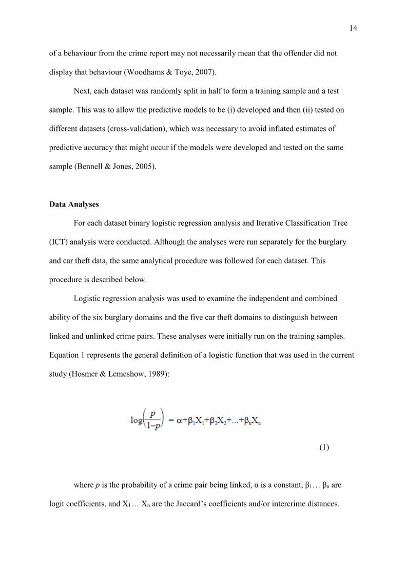
Equation 1 represents the general definition of a logistic function that was used in the current

study (Hosmer & Lemeshow, 1989):

(1)

where p is the probability of a crime pair being linked, α is a constant, β1… βn are

logit coefficients, and X1… Xn are the Jaccard’s coefficients and/or intercrime distances.

15

Separate direct logistic regression analyses were run for each behavioural domain, with the

similarity coefficient entered as an independent variable and linkage status (linked versus

unlinked) as the dichotomous dependent variable. Also, forward stepwise logistic regression

analysis was used to determine the optimal combination of domains for linkage purposes.

Excluding the combined domain, all behavioural domains were entered simultaneously in

these analyses. The combined domain was excluded to avoid violating the assumption of

multicollinearity (Field, 2009; Tonkin et al., 2011).

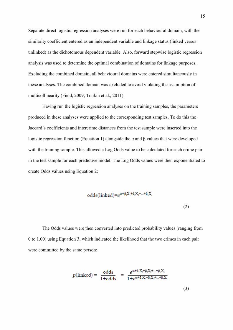
Having run the logistic regression analyses on the training samples, the parameters

produced in these analyses were applied to the corresponding test samples. To do this the

Jaccard’s coefficients and intercrime distances from the test sample were inserted into the

logistic regression function (Equation 1) alongside the α and β values that were developed

with the training sample. This allowed a Log Odds value to be calculated for each crime pair

in the test sample for each predictive model. The Log Odds values were then exponentiated to

create Odds values using Equation 2:

(2)

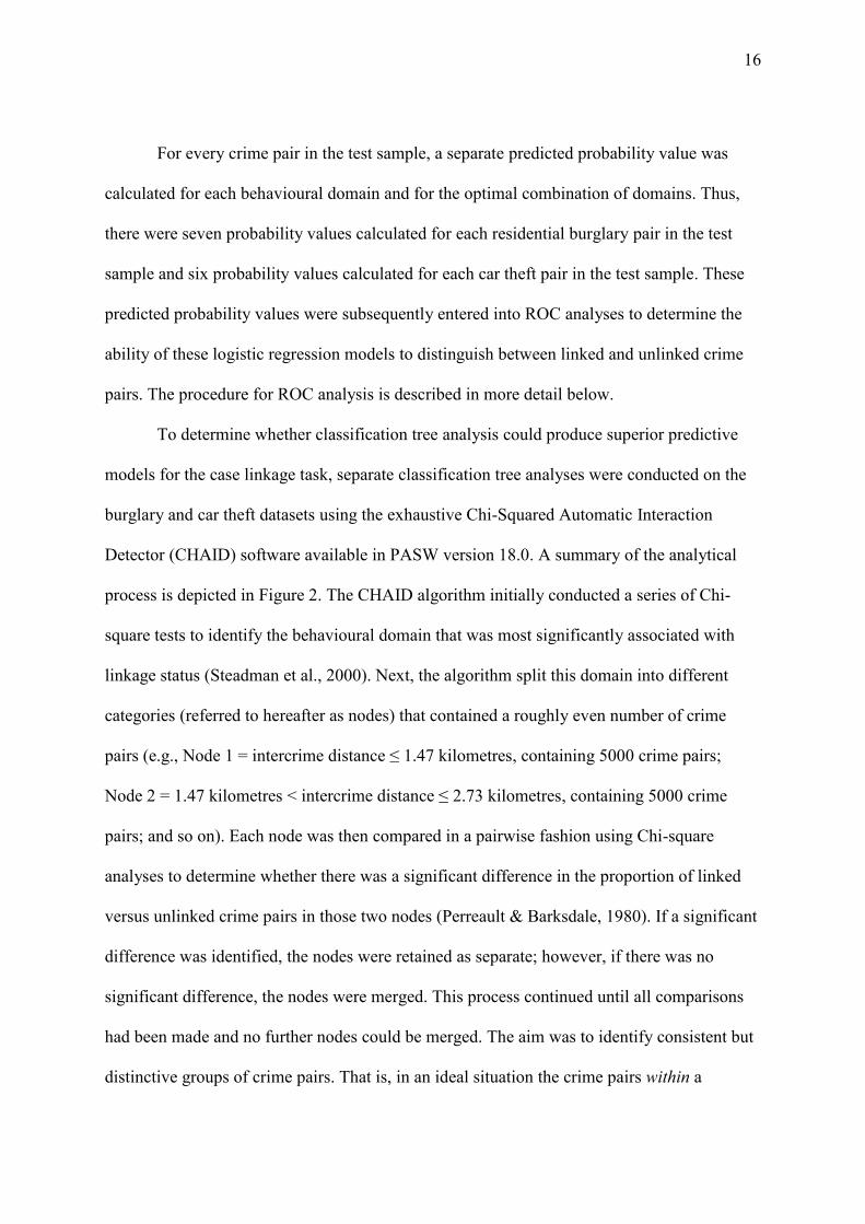
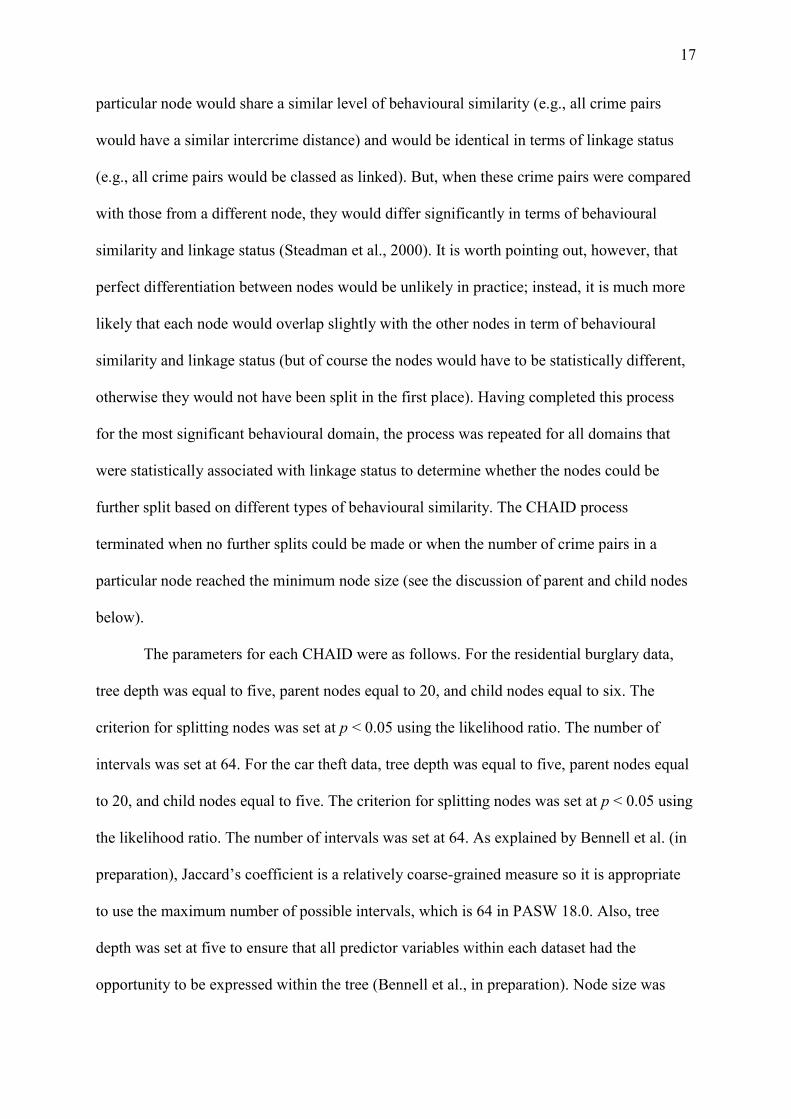
The Odds values were then converted into predicted probability values (ranging from

0 to 1.00) using Equation 3, which indicated the likelihood that the two crimes in each pair

were committed by the same person:

(3)

16

For every crime pair in the test sample, a separate predicted probability value was

calculated for each behavioural domain and for the optimal combination of domains. Thus,

there were seven probability values calculated for each residential burglary pair in the test

sample and six probability values calculated for each car theft pair in the test sample. These

predicted probability values were subsequently entered into ROC analyses to determine the

ability of these logistic regression models to distinguish between linked and unlinked crime

pairs. The procedure for ROC analysis is described in more detail below.

To determine whether classification tree analysis could produce superior predictive

models for the case linkage task, separate classification tree analyses were conducted on the

burglary and car theft datasets using the exhaustive Chi-Squared Automatic Interaction

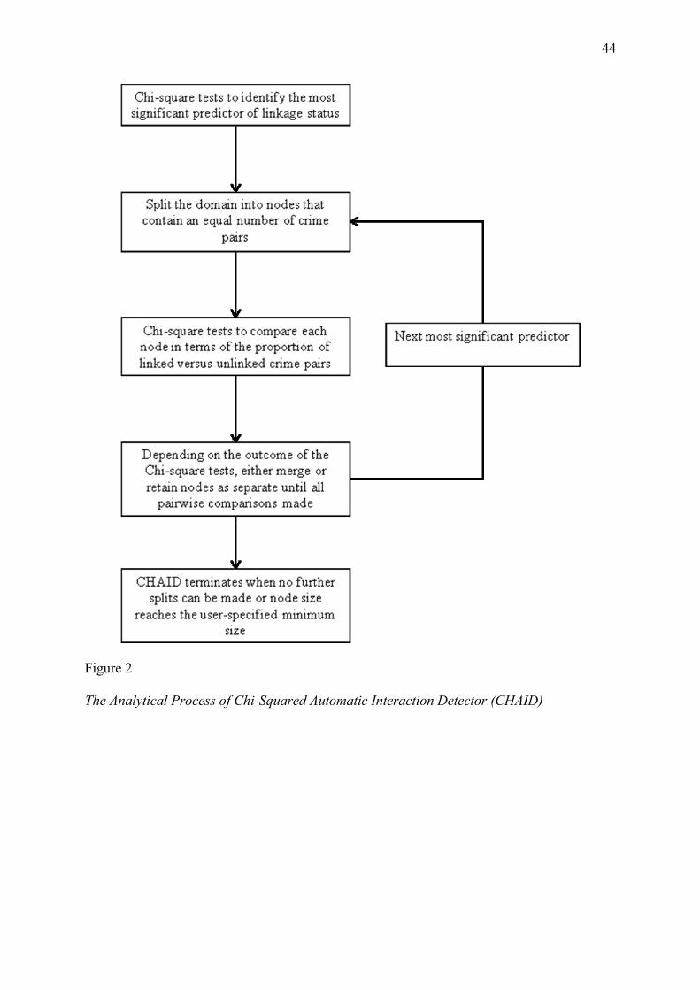
Detector (CHAID) software available in PASW version 18.0. A summary of the analytical

process is depicted in Figure 2. The CHAID algorithm initially conducted a series of Chi-

square tests to identify the behavioural domain that was most significantly associated with

linkage status (Steadman et al., 2000). Next, the algorithm split this domain into different

categories (referred to hereafter as nodes) that contained a roughly even number of crime

pairs (e.g., Node 1 = intercrime distance ≤ 1.47 kilometres, containing 5000 crime pairs;

Node 2 = 1.47 kilometres < intercrime distance ≤ 2.73 kilometres, containing 5000 crime

pairs; and so on). Each node was then compared in a pairwise fashion using Chi-square

analyses to determine whether there was a significant difference in the proportion of linked

versus unlinked crime pairs in those two nodes (Perreault & Barksdale, 1980). If a significant

difference was identified, the nodes were retained as separate; however, if there was no

significant difference, the nodes were merged. This process continued until all comparisons

had been made and no further nodes could be merged. The aim was to identify consistent but

distinctive groups of crime pairs. That is, in an ideal situation the crime pairs within a

17

particular node would share a similar level of behavioural similarity (e.g., all crime pairs

would have a similar intercrime distance) and would be identical in terms of linkage status

(e.g., all crime pairs would be classed as linked). But, when these crime pairs were compared

with those from a different node, they would differ significantly in terms of behavioural

similarity and linkage status (Steadman et al., 2000). It is worth pointing out, however, that

perfect differentiation between nodes would be unlikely in practice; instead, it is much more

likely that each node would overlap slightly with the other nodes in term of behavioural

similarity and linkage status (but of course the nodes would have to be statistically different,

otherwise they would not have been split in the first place). Having completed this process

for the most significant behavioural domain, the process was repeated for all domains that

were statistically associated with linkage status to determine whether the nodes could be

further split based on different types of behavioural similarity. The CHAID process

terminated when no further splits could be made or when the number of crime pairs in a

particular node reached the minimum node size (see the discussion of parent and child nodes

below).

The parameters for each CHAID were as follows. For the residential burglary data,

tree depth was equal to five, parent nodes equal to 20, and child nodes equal to six. The

criterion for splitting nodes was set at p < 0.05 using the likelihood ratio. The number of

intervals was set at 64. For the car theft data, tree depth was equal to five, parent nodes equal

to 20, and child nodes equal to five. The criterion for splitting nodes was set at p < 0.05 using

the likelihood ratio. The number of intervals was set at 64. As explained by Bennell et al. (in

preparation), Jaccard’s coefficient is a relatively coarse-grained measure so it is appropriate

to use the maximum number of possible intervals, which is 64 in PASW 18.0. Also, tree

depth was set at five to ensure that all predictor variables within each dataset had the

opportunity to be expressed within the tree (Bennell et al., in preparation). Node size was

18

based on previous comparative research with classification tree analysis and logistic

regression (Rosenfeld & Lewis, 2005; Thomas et al., 2005)5. The likelihood ratio was

selected because it is more robust than the alternative method, Pearson’s χ2 (SPSS, n.d.).

Following the criteria established by Steadman et al. (2000) and Monahan et al.

(2001), and subsequently used by Bennell et al. (in preparation), nodes containing less than

twice, but more than half, the base rate prevalence of linked pairs were deemed to be

unclassifiable. These unclassifiable cases were separated from those that were successfully

classified, and a further CHAID analysis was run on the unclassifiable cases. The same

analytical process depicted in Figure 2 and the same parameters described above were used in

the analysis. This iterative process was repeated until no further cases could be classified.

The SPSS sub-routine for classification tree analysis was used to develop a tree on the

training sample and then to automatically apply this tree to the test sample. These analyses

produced a predicted probability value for each crime pair in the training and test samples,

which were subsequently used to perform ROC analysis. This tested the discriminative

accuracy of the classification tree models.

ROC analysis provides an index of predictive accuracy (the AUC), which can range

from 0 (indicating perfect negative prediction) to 1.00 (indicating perfect positive prediction),

with a value of 0.50 indicating a chance level of accuracy. Typically, AUC values of 0.50 -

0.70 are considered low, values of 0.70 - 0.90 are moderate, and values of 0.90 - 1.00 are

high (Swets, 1988). ROC analysis is a useful measure of predictive accuracy because it

provides an estimate that is independent from specific decision thresholds (e.g., Bennell,

2005). Furthermore, the AUC is flexible in terms of being able to evaluate a wide variety of

offender behaviours and able to compare across samples that differ in terms of base rate and

composition (Bennell, 2002; Liu et al., 2011). This makes it well-suited to the current set of

analyses.

19

Separate ROC curves were constructed for each logistic regression model and the

classification tree model for the burglary and car theft datasets. These analyses provided an

insight into the relative ability of logistic regression and classification tree analysis to

construct predictive models for the purposes of case linkage. ROC curves were also

constructed for the training samples, as well as the test samples, to determine whether the

regression and classification tree models could be cross-validated. This is important in an

applied area of research such as this, where the ultimate aim is to develop findings that can be

applied to future police investigations. Furthermore, there is evidence to suggest that

classification tree models are less robust than regression models (e.g., Liu et al., 2011;

Rosenfeld & Lewis, 2005; Thomas et al., 2005), so it was important to examine this issue

with these data.

Results

Residential Burglary

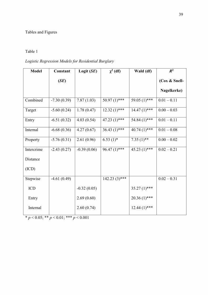
Six direct and one stepwise logistic regression analysis were conducted to examine

the ability of regression to build predictive models that could distinguish between linked and

unlinked crime pairs in the training sample. These findings are reported in Table 1. All

logistic regression models were statistically significant (p < 0.05), but the most successful

model (as measured by χ2) was the stepwise model that combined the intercrime distance,

entry behaviours, and internal behaviours. This was followed by the single-feature regression

model for the intercrime distance. These seven regression models were then applied to the

test sample to produce predicted probability values for the purposes of ROC analysis.

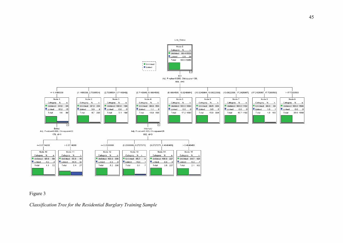
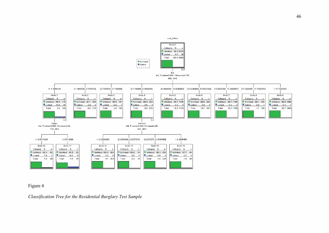
Classification tree analysis was also conducted on the training sample and

subsequently applied to the test sample. The classification trees produced by this analysis are

20

depicted in Figures 3 and 4. The same behavioural domains were included in the

classification tree model as the stepwise regression model (intercrime distance, entry

behaviours, and internal behaviours). According to the criteria of Steadman et al. (2000) and

Monahan et al. (2001), cases were categorised as unclassifiable when the percentage of

linked cases in a particular node fell between 0.30% and 1.20% for the training sample, and

between 0.35% and 1.40% for the test sample. Consequently, cases within nodes 4, 6, and 8

of the training sample and within nodes 3, 4, 6, 8, and 14 of the test sample were deemed

unclassifiable. This represented 2,604 crime pairs (20.47% of the total sample). A second

CHAID analysis was run on these unclassifiable cases, but no further cases could be

classified. The predicted probability values produced at iteration 1 were, therefore, used to

conduct ROC analysis.

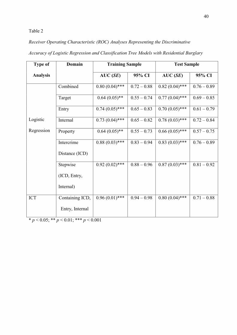
Eight ROC curves were constructed using the predicted probability values in the test

sample. Seven of these curves represented the logistic regression models reported in Table 1

and one represented the classification tree model. These analyses are reported in Table 2. All

models achieved statistically significant levels of discrimination accuracy (p < 0.001). The

most successful model with the test data appeared to be the stepwise regression model (AUC

= 0.87), which was superior to the classification tree model (AUC = 0.80). But, the

overlapping confidence intervals (CIs) indicate that this difference was not statistically

significant (Melnyk et al., 2010).

Also reported in Table 2 are the AUC values that were obtained using the training

sample. By comparing these AUC values with the equivalent values for the test sample, it is

possible to determine whether discrimination accuracy is robust using these statistical

models. With the exception of the target domain, the logistic regression models appear to be

robust and cross-validated. However, the classification tree model demonstrates a statistically

lower AUC value in the test sample compared to the training sample (as indicated by the non-

21

overlapping CIs; Melnyk et al., 2010). These findings suggest that the classification tree

model may not be as robust as the regression models when it comes to discriminating

between linked and unlinked residential burglaries in this sample.

There are several different techniques that can be used to counteract over-fitting (Loh

& Shih, 1997). For example, branches in the model that contain a relatively small number of

cases can be removed (this technique is referred to as pruning) and alterations can be made to

the model’s growth limits, such as decreasing the maximum tree depth and increasing the

minimum number of cases in the parent and child nodes (Liu et al., 2011). In an attempt to

make the burglary classification tree more robust, the criteria for splitting nodes was made

more stringent (p < 0.001) and the minimum number of cases allowed in the parent and child

nodes was increased to 100 and 50, respectively. These analyses produced a tree that was

much simpler than the initial tree, with the data split into nine nodes compared to the

previous 15 nodes and with just the intercrime distance used to make predictive decisions6. In

total, 3,703 pairs (29.11% of the total sample) were deemed unclassifiable. The iterative

process was unable to classify further cases, so the predicted probability values produced

using iteration 1 were used to construct ROC curves. These analyses produced an AUC value

of 0.93 (SE = 0.02, p < 0.001, 95% CI = 0.90 – 0.96) for the training sample and an AUC of

0.80 (SE = 0.04, p < 0.001, 95% CI = 0.72 – 0.89) for the test sample. The level of shrinkage

reduced slightly (from 0.16 to 0.13), but was still statistically significant (as indicated by the

non-overlapping CIs; Melnyk et al., 2010) and the classification tree model was still less

robust than most of the logistic regression models.

Car Theft

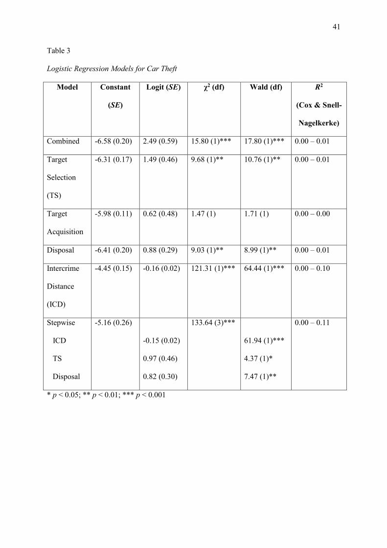
Five direct and one stepwise logistic regression analysis were conducted using the

training sample (see Table 3). All logistic regression models were statistically significant (p <

22

0.01), except the target acquisition model. The most successful model was the stepwise

model, which combined the intercrime distance, target selection choices, and disposal

behaviours. This was closely followed by the single-feature regression model for the

intercrime distance.

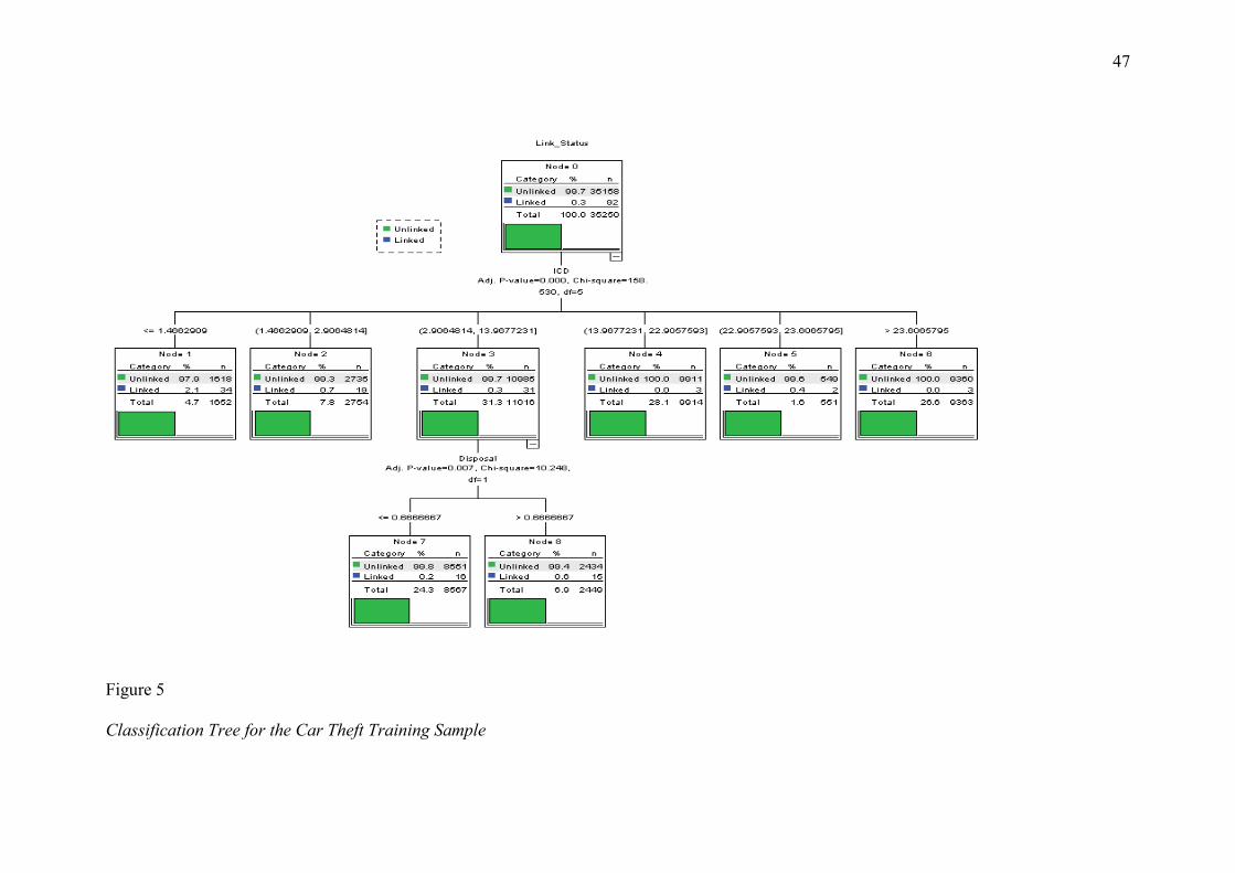
Classification tree analysis was also conducted on the training sample and

subsequently applied to the test sample. The classification trees produced by this analysis are

depicted in Figures 5 and 6. There was a slight difference in the behavioural domains

included in the tree-based model (the intercrime distance and disposal behaviours) compared

to the stepwise regression model (intercrime distance, target selection choices, and disposal

behaviours). Cases were categorised as unclassifiable when the percentage of linked cases in

a particular node fell between 0.15% and 0.60% for both the training and test samples.

Consequently, cases within nodes 3, 5, and 7 of the training sample and within nodes 2, 3, 7,

and 8 of the test sample were deemed unclassifiable. This represented 22,758 crime pairs

(32.28% of the total sample). A second CHAID analysis was run on these unclassifiable

cases, but no further cases could be classified. The predicted probability values produced at

iteration 1 were, therefore, used to conduct ROC analysis.

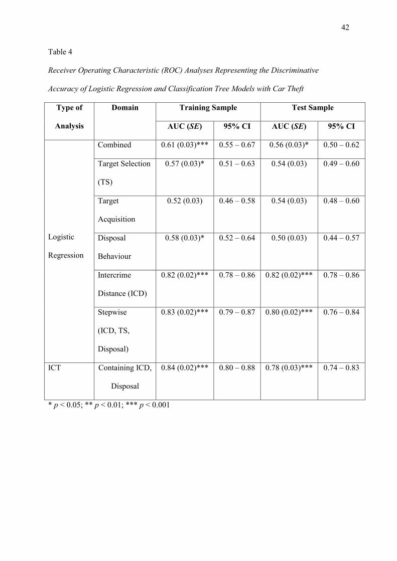
Seven ROC curves were constructed using the predicted probability values in the test

sample. Six of these curves represented the logistic regression models reported in Table 3 and

one represented the classification tree model. The ROC analyses are reported in Table 4. The

most successful model with the test data was the single-feature regression model using the

intercrime distance (AUC = 0.82). Somewhat unexpectedly this model outperformed the

stepwise regression model (AUC = 0.80), which can be explained by the reduction in

accuracy of the target selection and disposal domains when these regression models are

applied from the training data to the test data. In contrast, the intercrime distance retained a

stable level of predictive accuracy across both the training and test samples, thus allowing it

23

to outperform the stepwise model when applied to the test data. The conclusion that can be

drawn from these findings is that the intercrime distance is the most reliable logistic

regression model with these car theft data. The intercrime distance regression model also

outperformed the classification tree model, which achieved an AUC value of 0.78 with the

test data. But, the overlapping confidence intervals indicate that this difference was not

statistically significant (Melnyk et al., 2010).

In contrast to the residential burglary findings, there was little evidence to suggest

over-fitting with either the classification tree model or the intercrime distance regression

model.

Discussion

The purpose of the current study was to build on the novel work of Bennell et al. (in

preparation) by further comparing the ability of logistic regression analysis and classification

tree analysis to construct models of offender behaviour that can successfully discriminate

between linked and unlinked residential burglaries and car thefts. In both datasets

discrimination accuracy was found to be comparable between the regression- and tree-based

models; although the best regression models marginally outperformed the ICT models. These

findings are similar to those observed in the risk assessment literature (e.g., Gardner et al.,

1996; Liu et al., 2011) and the wider medical literature (e.g., Austin, 2007), where

comparable discrimination accuracy has been observed across various main effects and tree-

based regression approaches. They are also similar to those reported by Bennell et al. (in

preparation), who found comparable levels of discrimination accuracy when using logistic

regression and classification tree analysis to distinguish between linked and unlinked

burglaries, robberies, and rapes.

24

Given the greater transparency and usability of tree-based approaches, it might be

tempting to conclude from these findings that classification tree analysis is a favourable

alternative to logistic regression analysis. However, discrimination accuracy is only one

component of good model performance; another key component is reliability. That is, will the

model be able to discriminate successfully when it is applied to new cases that were not used

in its development?

The reliability findings differ for the residential burglary and car theft data. There was

significant shrinkage observed in the residential burglary sample when applying the

classification tree model from the training to test sample, which suggests that this model may

not fully generalise to new cases. This is a particular problem in applied research where the

ultimate aim is to develop predictive models that can be used to guide future investigations

and where incorrect linkage decisions can significantly hinder an investigation (Grubin et al.,

2001). Furthermore, it makes it difficult to provide an accurate estimate of the error rate one

should expect when using the burglary ICT model to identify linked and unlinked crimes.

Based on the 95% confidence intervals reported in Table 2, the estimate of discrimination

accuracy that an analyst might be expected to achieve using the ICT model to link residential

burglary crimes in Finland would range from 0.71 to 0.98. This is not a very precise estimate,

which may discourage the police and other law enforcement agencies from adopting these

models in practice.

However, the findings are more encouraging when we examine the best logistic

regression model for the burglary data (the intercrime distance). This model did not

demonstrate significant shrinkage from training to test, which suggests that it generalises to a

greater extent than the ICT model. Furthermore, it is possible to give a more precise estimate

of discrimination accuracy, which would range from 0.81 to 0.96 for the single-feature

intercrime distance model. Overall, these findings suggest that logistic regression is

25

favourable to classification tree analysis when constructing models for the purpose of linking

residential burglaries in this sample.

These findings differ to those reported by Bennell et al. (in preparation), thus

suggesting that we should be cautious before generalising their findings to other geographical

locations. This further supports the notion that replication-based research is an important

component of building a robust case linkage literature, as a multitude of social, demographic,

geographical, and pragmatic issues have the potential to alter case linkage findings (Tonkin et

al., 2011).

The over-fitting that was observed in the current sample of residential burglaries is

consistent with findings from the risk assessment literature, where complex predictive models

have sometimes failed to replicate when applied to new datasets (e.g., Liu et al., 2011;

Rosenfeld & Lewis, 2005; Thomas et al., 2005). It is particularly concerning that attempts to

counteract over-fitting with these data were unsuccessful. However, future research might

consider utilising different methods of cross-validation because the split-half method used in

the current study and by Bennell et al. (in preparation) may not be the most robust method for

testing the reliability of predictive models (Cohen, 1990). Alternatively, the multi-validation

methods described by Liu et al. (2011) and Grann and Långström (2007) might be of value.

Approaches such as these will help to ensure that the most robust classification tree is

constructed.

While we have discussed the reliability of the burglary models, we have not yet

discussed the car theft models. For these, both the classification tree model and the best

logistic regression model were reliable, with minimal shrinkage observed when

discrimination accuracy was compared across the training and test samples. These findings

are promising and suggest that classification tree analysis may offer an alternative to logistic

26

regression when building predictive models that can discriminate between linked and

unlinked car thefts.

These findings clearly differ from those with the burglary sample, where shrinkage

was observed from training to test when relying on the classification tree model to distinguish

between linked and unlinked crimes. A potential explanation is that the burglary tree was

more complex than the car theft tree, with three types of offender behaviour used to link

crime (compared with two in the car theft tree) and the data split across 15 nodes (compared

to eight in the car theft tree). In the context of case linkage, increasing model complexity can

be beneficial if it leads to a more refined understanding of real world offender behaviour, but

if the model becomes so complex that it begins to capture noise in the data and/or trends that

are unique to a particular sample this will lead to over-fitting (Liu et al., 2011). Arguably this

has happened with the burglary sample but not the car theft sample. It is, therefore, important

to determine why a more complex model emerged with the burglary sample. One possible

explanation is that the larger number of burglary (82) compared to car theft (44) variables

increased the potential for between-offender differences in behaviour, which would have led

to more nodes being formed when the CHAID algorithm was run on the burglary sample.

Alternatively, the burglary data may have been of better quality than the car theft data (as a

result of crime type or police procedures in Finland compared to the UK; see Tonkin et al.,

2011, for a more detailed discussion), which would also have allowed for greater between-

offender differences to emerge. Finally, it cannot be ruled out that the findings were due to

some quirk of these particular samples. Thus, future research should seek to determine

whether the findings replicate in other datasets.

A final issue that deserves attention is the proportion of unclassifiable cases that were

observed in the analyses. The classification tree model was unable to classify 32% of the car

theft crime pairs and 20% of the residential burglary pairs in this study. While these figures

27

are somewhat comparable to those reported in previous research (Bennell et al., in

preparation; Steadman et al., 2000), they are not insignificant numbers. Thus, if an analyst

were to utilise these trees in practice, the findings suggest that they would be unable to

proffer recommendations to investigating officers for approximately one in five residential

burglary crime pairs and one in three car theft pairs. This may limit their practical

applicability.

But, it is important to note that the percentage of unclassifiable cases is entirely

dependent on the criteria that are used to define what should and should not be classified. In

this study the criteria described by Steadman et al. (2000) and Monahan et al. (2001) were

adopted, so as to be consistent with Bennell et al. (in preparation) and the risk assessment

literature. However, it is unclear how Steadman, Monahan and colleagues developed these

criteria and, therefore, whether they are appropriate for use in a policing context. This is an

important issue because the most appropriate criteria for deciding whether cases can or

cannot be classified would depend on the situation in which linkage is being used. For

example, if the case linkage was to be presented as evidence in court, then the primary

concern would be to reach a reliable predictive decision. In this situation it would be

appropriate to adopt a strict set of criteria for judging whether a case is classifiable or not.

However, if the case linkage was to be used as an informal way of guiding an investigation,

then the primary concern may be to provide some sort of definite predictive decision

(whatever that may be). In this situation it may be appropriate to adopt less stringent criteria.

Thus, it should be clear from this discussion that, while the large number of unclassifiable

cases in this study is an important issue that should not be ignored, the practical impact of this

issue will differ considerably depending on the context in which case linkage is used during

police investigations.

28

In summary, while discrimination accuracy is relatively comparable across

classification tree and logistic regression models, classification tree models demonstrated

significant problems in terms of reliability or usability that the logistic regression models did

not experience. Based on these findings, the use of classification tree analysis as an

alternative to logistic regression cannot be supported in the area of behavioural case linkage

without further investigation. Primarily, this work should explore whether more robust

methods of cross-validation can help to build more reliable classification trees. This work can

continue with already-collected datasets, but there must be an attempt to test the relative

value of logistic regression and classification tree analysis with datasets from different

geographical locations that vary in terms of base rates and crime type. This will allow the

statistical procedures to be tested under varying conditions, which will increase the likelihood

that any conclusions drawn from this work will be applicable to a range of police forces and

other investigative agencies.

Another important area for future research is to test the usability of classification tree

models relative to logistic regression models. As discussed in the introduction, one of the key

advantages of classification tree analysis over logistic regression is its ease of use and

transparency (e.g., Steadman et al., 2000; Woodhams et al., 2011). But, this should not be

assumed; it should be explicitly tested with police crime analysts in mock linkage tasks, such

as those employed by Bennell, Bloomfield, Snook, Taylor, and Barnes (2010) and Santtila,

Korpela, and Häkkänen (2004).

Also, computational methods should be developed to calculate the temporal proximity

for all linked and unlinked pairs in a dataset, as is possible with the intercrime distance and

Jaccard’s coefficient. Temporal proximity has been shown to facilitate moderate levels of

discrimination accuracy with samples of residential burglary and car theft (Davies, Tonkin,

29

Bull, & Bond, submitted; Markson et al., 2010; Tonkin et al., 2011), so the exclusion of this

domain from the analyses in this study is clearly a limitation.

Furthermore, future work should attempt to examine the value of classification tree

analysis using samples of unsolved crime, which better reflect the real-life situation in which

case linkage is expected to perform (e.g., Woodhams & Labuschagne, 2011). This will help

to overcome a limitation that the current study and Bennell et al. (in preparation) share by

utilising samples of solved crime. However, the relatively large sample sizes that are needed

to conduct classification tree analysis (Perreault & Barksdale, 1980) probably mean that this

work will need to involve several different police forces.

Finally, future research with logistic regression and classification tree analysis should

explore the impact of sampling all offences in an offender’s crime series, rather than

restricting the analysis to just two offences per offender (as was the case in this study). As

explained by Woodhams and Labuschagne (2011), police crime databases contain series of

varying length and to sample a constant number of offences per offender may not provide the

most realistic test of behavioural case linkage. By conducting research using both

methodologies, the literature will hopefully obtain a balance between controlling the

influence of prolific offenders and testing case linkage in a more realistic manner.

Despite these limitations, this study has built on the novel work of Bennell et al. (in

preparation). The current findings suggest that researchers and practitioners should be

cautious if they are considering using classification trees to identify series of linked offences.

A significant amount of empirical work is needed to determine whether the problems of

reliability and usability identified in this study can be overcome and, therefore, whether

classification tree analysis represents a viable alternative to logistic regression analysis.

30

Footnotes

1 Please refer to the Method section for a more detailed description of this methodology.

2 Control behaviours were defined as those behaviours that allow the offender to carry out a given offence

exactly as they would wish without disruption, including variables such as the number of offenders and the level

of violence used. Planning behaviours were those that indicated the offender/s had put some thought into

conducting the offence prior to actually committing the robbery (e.g., wearing a disguise, using a getaway

vehicle, and bringing a bag to carry stolen goods away). The intercrime distance was the number of kilometres

separating offence locations. Research has suggested that crimes committed by the same person will be

committed in closer geographical proximity than crimes committed by different persons (e.g., Bennell & Canter,

2002).

3 These calculations are described in detail during the Method section of this paper.

4 The greater Helsinki region of Finland covers an area of approximately 815KM2 that contains the capital of

Finland, Helsinki, and the neighbouring cities of Espoo and Vantaa.

5 However, it should be noted that there are many- sometimes contradictory- recommendations regarding the

appropriate size of parent and child nodes.

6 The classification tree can be obtained upon request from the first author.

31

References

Austin, P. C. (2007). A comparison of regression trees, logistic regression, generalized

additive models, and multivariate adaptive regression splines for predicting AMI

mortality. Statistics in Medicine, 26, 2937-2957. doi: 10.1002/sim.2770

Bennell, C. (2002). Behavioural consistency and discrimination in serial burglary

(Unpublished doctoral dissertation). University of Liverpool, Liverpool, UK.

Bennell, C. (2005). Improving police decision making: General principles and practical

applications of Receiver Operating Characteristic analysis. Applied Cognitive

Psychology, 19, 1157-1175. doi: 10.1002/acp.1152

Bennell, C., Bloomfield, S., Snook, B., Taylor, P., & Barnes, C. (2010). Linkage analysis in

cases of serial burglary: Comparing the performance of university students, police

professionals, and a logistic regression model. Psychology, Crime & Law, 16, 507-

524. doi: 10.1080/10683160902971030

Bennell, C., & Canter, D. V. (2002). Linking commercial burglaries by modus operandi:

Tests using regression and ROC analysis. Science and Justice, 42, 153-164. doi:

10.1016/S1355-0306(02)71820-0

Bennell, C., & Jones, N. J. (2005). Between a ROC and a hard place: A method for linking

serial burglaries by modus operandi. Journal of Investigative Psychology and

Offender Profiling, 2, 23-41. doi: 10.1002/jip.21

32

Bennell, C., Jones, N. J., & Melnyk, T. (2009). Addressing problems with traditional crime

linking methods using receiver operating characteristic analysis. Legal and

Criminological Psychology, 14, 293-310. doi: 10.1348/135532508X349336

Bennell, C., Woodhams, J., & Beauregard, E. (in preparation). Investigating individual

differences in the expression of behavioural consistency in crime series using ICT

analyses.

Canter, D., & Heritage, R. (1990). A multivariate model of sexual offences behavior:

Developments in offender profiling. Journal of Forensic Psychiatry, 1, 185-212. doi:

10.1080/09585189008408469

Charron, A., & Woodhams, J. (2010). A qualitative analysis of mock jurors’ deliberations of

linkage analysis evidence. Journal of Investigative Psychology and Offender

Profiling, 7, 165-183. doi: 10.1002/jip.119

Cohen, J. (1990). Things I have learned (so far). American Psychologist, 45, 1304-1312. doi:

10.1037/0003-066X.45.12.1304

Davies, K., Tonkin, M., Bull, R., & Bond, J. W. (submitted). The course of case linkage

never did run smooth: A new investigation to tackle the behavioural changes in serial

car theft.

Field, A. (2009). Discovering statistics using SPSS (3rd ed.). London, UK: Sage.

33

Gardner, W., Lidz, C. W., Mulvey, E. P., & Shaw, E. C. (1996). A comparison of actuarial

methods for identifying repetitively violent patients with mental illnesses. Law and

Human Behavior, 20, 35-48. doi:10.1007/BF01499131

Grann, M., & Långström, N. (2007). Actuarial assessment of violence risk: To weigh or not

to weigh? Criminal Justice and Behavior, 34, 22-36. doi:

10.1177/0093854806290250

Grubin, D., Kelly, P., & Brunsdon, C. (2001). Linking serious sexual assaults through

behaviour (Home Office Research Study 215). London, UK: Home Office Research,

Development and Statistics Directorate.

Hazelwood, R. R., & Warren, J. I. (2003). Linkage analysis: Modus operandi, ritual, and

signature in serial sexual crime. Aggression and Violent Behavior, 8, 587-598. doi:

10.1016/S1359-1789(02)00106-4

Hosmer, D. W., & Lemeshow, S. (1989). Applied logistic regression. New York, NY: Wiley.

Kinnear, P. R., & Gray, C. D. (2009). SPSS 16 made simple. Hove, UK: Psychology Press.

Labuschagne, G. (2012). The use of a linkage analysis as an investigative tool and evidential

material in serial offenses. In K. Borgeson & K. Kuehnle (Eds.), Serial offenders:

Theory and practice (pp. 187-215). Sudbury, MA: Jones & Bartlett Learning.

34

Laukkanen, M., Santtila, P., Jern, P., & Sandnabba, K. (2008). Predicting offender home

location in urban burglary series. Forensic Science International, 176, 224-235. doi:

10.1016/j.forsciint.2007.09.011

Liu, Y. Y., Yang, M., Ramsay, M., Li, X. S., & Coid, J. W. (2011). A comparison of logistic

regression, classification and regression tree, and neural networks models in

predicting violent re-offending. Journal of Quantitative Criminology. Advance online

publication. doi: 10.1007/s10940-011-9137-7

Loh, W. Y., & Shih, Y. S. (1997). Split selection methods for classification trees. Statistica

Sinica, 7, 815-840. doi: 10.1.1.127.7375

Markson, L., Woodhams, J., & Bond, J. W. (2010). Linking serial residential burglary:

Comparing the utility of modus operandi behaviours, geographical proximity, and

temporal proximity. Journal of Investigative Psychology and Offender Profiling, 7,

91-107. doi: 10.1002/jip.120

Melnyk, T., Bennell, C., Gauthier, D. J., & Gauthier, D. (2010). Another look at across-crime

similarity coefficients for use in behavioural linkage analysis: An attempt to replicate

Woodhams, Grant, and Price (2007). Psychology, Crime & Law, 17, 359-380. doi:

10.1080/10683160903273188

Monahan, J., Steadman, H. J., Silver, E., Appelbaum, P. S., Clark Robbins, P., Mulvey, E. P.,

… Banks, S. (2001). Rethinking risk assessment: The MacArthur study of mental

disorder and violence. Oxford, UK: Oxford University Press.

35

Peduzzi, P., Concato, J., Kemper, E., Holford, T. R., & Feinstein, A. R. (1996). A simulation

study of the number of events per variable in logistic regression analysis. Journal of

Clinical Epidemiology, 49, 1373-1379. doi: 10.1016/S0895-4356(96)00236-3

Perreault, W. D., Jr., & Barksdale, H. C., Jr. (1980). A model-free approach for analysis of

complex contingency data in survey research. Journal of Marketing Research, 17,

503-515. doi:10.2307/3150503

Rosenfeld, B., & Lewis, C. (2005). Assessing violence risk in stalking cases: A regression

tree approach. Law and Human Behavior, 29, 343-357. doi: 10.1007/s10979-005-

3318-6

Santtila, P., Fritzon, K., & Tamelander, A. L. (2004). Linking serial arson incidents on the

basis of crime scene behavior. Journal of Police and Criminal Psychology, 19, 1-16.

doi: 10.1007/BF02802570

Santtila, P., Junkkila, J., & Sandnabba, N. K. (2005). Behavioural linking of stranger rapes.

Journal of Investigative Psychology and Offender Profiling, 2, 87-103. doi:

10.1002/jip.26

Santtila, P., Korpela, S., & Häkkänen, H. (2004). Expertise and decision-making in the

linking of car crime series. Psychology, Crime & Law, 10, 97-112. doi:

10.1080/1068316021000030559

36

Santtila, P., Ritvanen, A., & Mokros, A. (2004). Predicting burglar characteristics from crime

scene behaviour. International Journal of Police Science & Management, 6, 136-154.

doi:10.1350/ijps.6.3.136.39127

SPSS (n.d.). PASW decision trees 18. Retrieved from

http://www.sussex.ac.uk/its/pdfs/SPSS18_Decision_Trees.pdf

Steadman, H. J., Silver, E., Monahan, J., Appelbaum, P. S., Clark Robbins, P., Mulvey, E. P.,

… Banks, S. (2000). A classification tree approach to the development of actuarial

violence risk assessment tools. Law and Human Behavior, 24, 83-100. doi:

10.1023/A:1005478820425

Swets, J. A. (1988). Measuring the accuracy of diagnostic systems. Science, 240, 1285-1293.

doi: 10.1126/science.3287615

Thomas, S., Leese, M., Walsh, E., McCrone, P., Moran, P., Burns, T., … Fahy, T. (2005). A

comparison of statistical models in predicting violence in psychotic illness.

Comprehensive Psychiatry, 46, 296-303. doi: 10.1016/j.comppsych.2004.10.001

Tonkin, M. (2007). To link or not to link: A test of the case linkage principles using serial car

theft data (Unpublished Masters’ dissertation). University of Leicester, Leicester, UK.

Tonkin, M., Grant, T., & Bond, J. W. (2008). To link or not to link: A test of the case linkage

principles using serial car theft data. Journal of Investigative Psychology and

Offender Profiling, 5, 59-77. doi: 10.1002/jip.74

37

Tonkin, M., Santtila, P., & Bull, R. (2011). The linking of burglary crimes using offender

behavior: Testing research cross-nationally and in more realistic settings. Legal and

Criminological Psychology. Advance online publication. doi: 10.1111/j.2044-

8333.2010.02007.x

Woodhams, J. (2008). Juvenile sex offending: An investigative perspective (Unpublished

doctoral dissertation). University of Leicester, Leicester, UK.

Woodhams, J., Bennell, C., & Beauregard, E. (2011, June). Are all serial rapists consistent in

the same way? In M. Tonkin (Chair), Linking crimes using offender behaviour: New

and emerging directions for research. Symposium conducted at the 20th Annual

Division of Forensic Psychology Conference 2011, Portsmouth, UK.

Woodhams, J., Grant, T. D., & Price, A. R. G. (2007). From marine ecology to crime

analysis: Improving the detection of serial sexual offences using a taxonomic

similarity measure. Journal of Investigative Psychology and Offender Profiling, 4, 17-

27. doi: 10.1002/jip.55

Woodhams, J., Hollin, C. R., & Bull, R. (2007). The psychology of linking crimes: A review

of the evidence. Legal and Criminological Psychology, 12, 233-249. doi:

10.1348/135532506X118631

38

Woodhams, J., & Labuschagne, G. (2011). A test of case linkage principles with solved and

unsolved serial rapes. Journal of Police and Criminal Psychology. Advance online

publication. doi: 10.1007/s11896-011-9091-1

Woodhams, J., & Toye, K. (2007). An empirical test of the assumptions of case linkage and

offender profiling with serial commercial robberies. Psychology, Public Policy, and

Law, 13, 59-85. doi: 10.1037/1076-8971.13.1.59

39

Tables and Figures

Table 1

Logistic Regression Models for Residential Burglary

Model Constant

(SE)

Logit (SE) χ2 (df) Wald (df) R2

(Cox & Snell-

Nagelkerke)

Combined -7.30 (0.39) 7.87 (1.03) 50.97 (1)*** 59.05 (1)*** 0.01 – 0.11

Target -5.60 (0.24) 1.78 (0.47) 12.32 (1)*** 14.47 (1)*** 0.00 – 0.03

Entry -6.51 (0.32) 4.03 (0.54) 47.23 (1)*** 54.84 (1)*** 0.01 – 0.11

Internal -6.68 (0.36) 4.27 (0.67) 36.43 (1)*** 40.74 (1)*** 0.01 – 0.08

Property -5.76 (0.31) 2.61 (0.96) 6.53 (1)* 7.35 (1)** 0.00 – 0.02

Intercrime

Distance

(ICD)

-2.43 (0.27) -0.39 (0.06) 96.47 (1)*** 45.23 (1)*** 0.02 – 0.21

Stepwise

ICD

Entry

Internal

-4.61 (0.49)

-0.32 (0.05)

2.69 (0.60)

2.60 (0.74)

142.23 (3)***

35.27 (1)***

20.36 (1)***

12.44 (1)***

0.02 – 0.31

* p < 0.05; ** p < 0.01; *** p < 0.001

40

Table 2

Receiver Operating Characteristic (ROC) Analyses Representing the Discriminative

Accuracy of Logistic Regression and Classification Tree Models with Residential Burglary

Type of

Analysis

Domain Training Sample Test Sample

AUC (SE) 95% CI AUC (SE) 95% CI

Logistic

Regression

Combined 0.80 (0.04)*** 0.72 – 0.88 0.82 (0.04)*** 0.76 – 0.89

Target 0.64 (0.05)** 0.55 – 0.74 0.77 (0.04)*** 0.69 – 0.85

Entry 0.74 (0.05)*** 0.65 – 0.83 0.70 (0.05)*** 0.61 – 0.79

Internal 0.73 (0.04)*** 0.65 – 0.82 0.78 (0.03)*** 0.72 – 0.84

Property 0.64 (0.05)** 0.55 – 0.73 0.66 (0.05)*** 0.57 – 0.75

Intercrime

Distance (ICD)

0.88 (0.03)*** 0.83 – 0.94 0.83 (0.03)*** 0.76 – 0.89

Stepwise

(ICD, Entry,

Internal)

0.92 (0.02)*** 0.88 – 0.96 0.87 (0.03)*** 0.81 – 0.92

ICT Containing ICD,

Entry, Internal

0.96 (0.01)*** 0.94 – 0.98 0.80 (0.04)*** 0.71 – 0.88

* p < 0.05; ** p < 0.01; *** p < 0.001

41

Table 3

Logistic Regression Models for Car Theft

Model Constant

(SE)

Logit (SE) χ2 (df) Wald (df) R2

(Cox & Snell-

Nagelkerke)

Combined -6.58 (0.20) 2.49 (0.59) 15.80 (1)*** 17.80 (1)*** 0.00 – 0.01

Target

Selection

(TS)

-6.31 (0.17) 1.49 (0.46) 9.68 (1)** 10.76 (1)** 0.00 – 0.01

Target

Acquisition

-5.98 (0.11) 0.62 (0.48) 1.47 (1) 1.71 (1) 0.00 – 0.00

Disposal -6.41 (0.20) 0.88 (0.29) 9.03 (1)** 8.99 (1)** 0.00 – 0.01

Intercrime

Distance

(ICD)

-4.45 (0.15) -0.16 (0.02) 121.31 (1)*** 64.44 (1)*** 0.00 – 0.10

Stepwise

ICD

TS

Disposal

-5.16 (0.26)

-0.15 (0.02)

0.97 (0.46)

0.82 (0.30)

133.64 (3)***

61.94 (1)***

4.37 (1)*

7.47 (1)**

0.00 – 0.11

* p < 0.05; ** p < 0.01; *** p < 0.001

42

Table 4

Receiver Operating Characteristic (ROC) Analyses Representing the Discriminative

Accuracy of Logistic Regression and Classification Tree Models with Car Theft

Type of

Analysis

Domain Training Sample Test Sample

AUC (SE) 95% CI AUC (SE) 95% CI

Logistic

Regression

Combined 0.61 (0.03)*** 0.55 – 0.67 0.56 (0.03)* 0.50 – 0.62

Target Selection

(TS)

0.57 (0.03)* 0.51 – 0.63 0.54 (0.03) 0.49 – 0.60

Target

Acquisition

0.52 (0.03) 0.46 – 0.58 0.54 (0.03) 0.48 – 0.60

Disposal

Behaviour

0.58 (0.03)* 0.52 – 0.64 0.50 (0.03) 0.44 – 0.57

Intercrime

Distance (ICD)

0.82 (0.02)*** 0.78 – 0.86 0.82 (0.02)*** 0.78 – 0.86

Stepwise

(ICD, TS,

Disposal)

0.83 (0.02)*** 0.79 – 0.87 0.80 (0.02)*** 0.76 – 0.84

ICT Containing ICD,

Disposal

0.84 (0.02)*** 0.80 – 0.88 0.78 (0.03)*** 0.74 – 0.83

* p < 0.05; ** p < 0.01; *** p < 0.001

43

Figure 1

A Hypothetical Classification Tree for Commercial Robbery

44

Figure 2

The Analytical Process of Chi-Squared Automatic Interaction Detector (CHAID)

45

Figure 3

Classification Tree for the Residential Burglary Training Sample

46

Figure 4

Classification Tree for the Residential Burglary Test Sample

47

Figure 5

Classification Tree for the Car Theft Training Sample

48

Figure 6

Classification Tree for the Car Theft Test Sample