from predictive to prescriptive analytics · from predictive to prescriptive analytics dimitris...
TRANSCRIPT

From Predictive to Prescriptive Analytics
Dimitris BertsimasSloan School of Management, Massachusetts Institute of Technology, Cambridge, MA 02139, [email protected]
Nathan KallusSchool of Operations Research and Information Engineering and Cornell Tech, Cornell University, New York, NY 11109,
In this paper, we combine ideas from machine learning (ML) and operations research and management
science (OR/MS) in developing a framework, along with specific methods, for using data to prescribe optimal
decisions in OR/MS problems. In a departure from other work on data-driven optimization and reflecting
our practical experience with the data available in applications of OR/MS, we consider data consisting,
not only of observations of quantities with direct e↵ect on costs/revenues, such as demand or returns, but
predominantly of observations of associated auxiliary quantities. The main problem of interest is a conditional
stochastic optimization problem, given imperfect observations, where the joint probability distributions
that specify the problem are unknown. We demonstrate that our proposed solution methods, which are
inspired by ML methods such as local regression (LOESS), classification and regression trees (CART), and
random forests (RF), are generally applicable to a wide range of decision problems. We prove that they
are computationally tractable and asymptotically optimal under mild conditions even when data is not
independent and identically distributed (iid) and even for censored observations. We extend these results
to the case where some of the decision variables can directly a↵ect uncertainty in unknown ways, such
as pricing’s e↵ect on demand in joint pricing and planning problems. As an analogue to the coe�cient of
determination R2, we develop a metric P termed the coe�cient of prescriptiveness to measure the prescriptive
content of data and the e�cacy of a policy from an operations perspective. To demonstrate the power of
our approach in a real-world setting we study an inventory management problem faced by the distribution
arm of an international media conglomerate, which ships an average of 1 billion units per year. We leverage
both internal data and public online data harvested from IMDb, Rotten Tomatoes, and Google to prescribe
operational decisions that outperform baseline measures. Specifically, the data we collect, leveraged by our
methods, accounts for an 88% improvement as measured by our coe�cient of prescriptiveness.
1. Introduction
In today’s data-rich world, many problems of operations research and management science
(OR/MS) can be characterized by three primitives:
a) Data {y1, . . . , yN} on uncertain quantities of interest Y 2 Y ⇢ Rdy such as simultaneous
demands.
b) Auxiliary data {x1, . . . , xN} on associated covariates X 2 X ⇢ Rdx such as recent sale figures,
volume of Google searches for a products or company, news coverage, or user reviews, where xi
is concurrently observed with yi.
1
arX
iv:1
402.
5481
v4 [
stat
.ML
] 1
9 Ju
l 201
8

Bertsimas and Kallus:2 From Predictive to Prescriptive Analytics
c) A decision z constrained in Z ⇢ Rdz made after some observation X = x with the objective of
minimizing the uncertain costs c(z;Y ).
Traditionally, decision-making under uncertainty in OR/MS has largely focused on the problem
vstoch = minz2Z E [c(z;Y )] , zstoch 2 argminz2Z E [c(z;Y )] (1)
and its multi-period generalizations and addressed its solution under a priori assumptions about
the distribution µY of Y (cf. Birge and Louveaux (2011)), or, at times, in the presence of data
{y1, . . . , yn} in the assumed form of independent and identically distributed (iid) observations
drawn from µY (cf. Shapiro (2003), Shapiro and Nemirovski (2005), Kleywegt et al. (2002)). (We
will discuss examples of (1) in Section 1.1.) By and large, auxiliary data {x1, . . . , xN} has not been
extensively incorporated into OR/MS modeling, despite its growing influence in practice.
From its foundation, machine learning (ML), on the other hand, has largely focused on supervised
learning, or the prediction of a quantity Y (usually univariate) as a function of X, based on
data {(x1, y1), . . . , (xN , yN)}. By and large, ML does not address optimal decision-making under
uncertainty that is appropriate for OR/MS problems.
At the same time, an explosion in the availability and accessibility of data and advances in
ML have enabled applications that predict, for example, consumer demand for video games (Y )
based on online web-search queries (X) (Choi and Varian (2012)) or box-o�ce ticket sales (Y )
based on Twitter chatter (X) (Asur and Huberman (2010)). There are many other applications of
ML that proceed in a similar manner: use large-scale auxiliary data to generate predictions of a
quantity that is of interest to OR/MS applications (Goel et al. (2010), Da et al. (2011), Gruhl et al.
(2005, 2004), Kallus (2014)). However, it is not clear how to go from a good prediction to a good
decision. A good decision must take into account uncertainty wherever present. For example, in the
absence of auxiliary data, solving (1) based on data {y1, . . . , yn} but using only the sample mean
y = 1N
PN
i=1 yi ⇡E [Y ] and ignoring all other aspects of the data would generally lead to inadequate
solutions to (1) and an unacceptable waste of good data.
In this paper, we combine ideas from ML and OR/MS in developing a framework, along with
specific methods, for using data to prescribe optimal decisions in OR/MS problems that leverage
auxiliary observations. Specifically, the problem of interest is
v⇤(x) = minz2Z E⇥c(z;Y )
��X = x⇤, z⇤(x)2Z⇤(x) = argminz2Z E
⇥c(z;Y )
��X = x⇤, (2)
where the underlying distributions are unknown and only data SN = {(x1, y1), . . . , (xN , yN)} is
available. The solution z⇤(x) to (2) represents the full-information optimal decision, which, via full
knowledge of the unknown joint distribution µX,Y of (X, Y ), leverages the observation X = x to
the fullest possible extent in minimizing costs. We use the term predictive prescription for any
Bertsimas and Kallus:From Predictive to Prescriptive Analytics 3
function z(x) that prescribes a decision in anticipation of the future given the observation X = x.
Our task is to use SN to construct a data-driven predictive prescription zN(x). Our aim is that its
performance in practice, E⇥c(zN(x);Y )
��X = x⇤, is close to the full-information optimum, v⇤(x).
Our key contributions include:
a) We propose various ways for constructing predictive prescriptions zN(x) The focus of the paper
is predictive prescriptions that have the form
zN(x)2 argminz2ZPN
i=1 wN,i(x)c(z;yi), (3)
where wN,i(x) are weight functions derived from the data. We motivate specific constructions
inspired by a great variety of predictive ML methods, including for example and random forests
(RF; Breiman (2001)). We briefly summarize a selection of these constructions that we find the
most e↵ective below.
b) We also consider a construction motivated by the traditional empirical risk minimization (ERM)
approach to ML. This construction has the form
zN(·)2 argminz(·)2F1N
PN
i=1 c(z(xi);yi), (4)
where F is some class of functions. We extend the standard ML theory of out-of-sample guar-
antees for ERM to the case of multivariate-valued decisions encountered in OR/MS problems.
We find, however, that in the specific context of OR/MS problems, the construction (4) su↵ers
from some limitations that do not plague the predictive prescriptions derived from (3).
c) We show that that our proposals are computationally tractable under mild conditions.
d) We study the asymptotics of our proposals under sampling assumptions more gen-
eral than iid by leveraging universal law-of-large-number results of Walk (2010). Under
appropriate conditions and for certain predictive prescriptions zN(x) we show that costs
with respect to the true distributions converge to the full information optimum, i.e.,
limN!1 E⇥c(zN(x);Y )
��X = x⇤= v⇤(x), and that prescriptions converge to true full information
optimizers, i.e., limN!1 infz2Z⇤(x) ||z � zN(x)|| = 0, both for almost everywhere x and almost
surely. We extend our results to the case of censored data (such as observing demand via sales).
e) We extend the above results to the case where some of the decision variables may a↵ect the
uncertain variable in unknown ways not encapsulated in the known cost function. In this case,
the uncertain variable Y (z) will be di↵erent depending on the decision and the problem of
interest becomes minz2Z E⇥c(z;Y (z))
��X = x⇤. Complicating the construction of a data-driven
predictive prescription, however, is that the data only includes the realizations Yi = Yi(Zi)
corresponding to historic decisions. For example, in problems that involve pricing decisions such
as simultaneous planning and pricing, price has an unknown causal e↵ect on demand that must

Bertsimas and Kallus:4 From Predictive to Prescriptive Analytics
be determined in order to optimize the full decision z, which includes prices and production or
shipment plans, and the data only includes demand realized at particular historical prices. We
show that under certain conditions our methods can be extended to this case while perserving
favorable asymptotic properties.
f) We introduce a new metric P , termed the coe�cient of prescriptiveness, in order to measure the
e�cacy of a predictive prescription and to assess the prescriptive content of covariates X, that
is, the extent to which observing X is helpful in reducing costs. An analogue to the coe�cient of
determination R2 of predictive analytics, P is a unitless quantity that is (eventually) bounded
between 0 (not prescriptive) and 1 (highly prescriptive).
g) We demonstrate in a real-world setting the power of our approach. We study an inventory man-
agement problem faced by the distribution arm of an international media conglomerate. This
entity manages over 0.5 million unique items at some 50,000 retail locations around the world,
with which it has vendor-managed inventory (VMI) and scan-based trading (SBT) agreements.
On average it ships about 1 billion units a year. We leverage both internal company data and, in
the spirit of the aforementioned ML applications, large-scale public data harvested from online
sources, including IMDb, Rotten Tomatoes, and Google Trends. These data combined, leveraged
by our approach, lead to large improvements in comparison to baseline measures, in particular
accounting for an 88% improvement toward the deterministic perfect-foresight counterpart.
Of our proposed constructions of predictive prescriptions zN(x), the ones that we find to be
generally the most broadly and practically e↵ective are the following:
a) Motivated by k-nearest-neighbors regression (kNN; Altman (1992)),
zkNNN (x)2 argminz2Z
Pi2Nk(x) c(z;yi), (5)
where Nk(x) = {i = 1, . . . ,N :PN
j=1 I [||x�xi||� ||x�xj||] k} is the neighborhood of the k
data points that are closest to x.
b) Motivated by local linear regression (LOESS; Cleveland and Devlin (1988)),
zLOESS*N (x)2 argminz2Z
Pn
i=1 ki(x)max{1�Pn
j=1 kj(x)(xj �x)T⌅(x)�1(xi �x),0}c(z;yi), (6)
where ⌅(x) =Pn
i=1 ki(x)(xi�x)(xi�x)T , ki(x) = (1� (||xi �x||/hN(x))3)3 I [||xi �x|| hN(x)],
and hN(x) > 0 is the distance to the k-nearest point from x. Although this form may seem
complicated, it (nearly) corresponds to the simple idea of approximating E⇥c(z;Y )
��X = x⇤
locally by a linear function in x, which we will discuss at greater length in Section 2.
c) Motivated by classification and regression trees (CART; Breiman et al. (1984)),
zCARTN (x)2 argminz2Z
Pi:R(xi)=R(x) c(z;yi), (7)
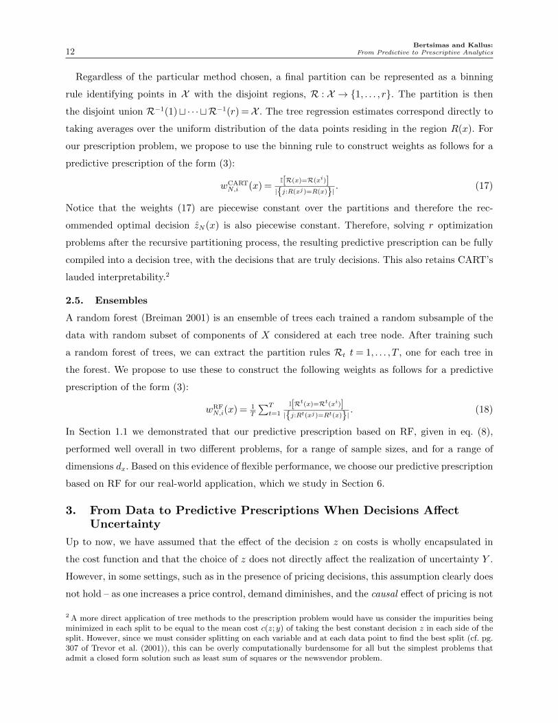
where R(x) is the binning rule implied by a regression tree trained on the data SN as shown in
an example in Figure 1.

Bertsimas and Kallus:From Predictive to Prescriptive Analytics 5
Figure 1 A regression tree is trained on data�(x1, y1), . . . , (x10, y10)
and partitions the X data into regions
defined by the leaves. The Y prediction m(x) is mj , the average of Y data at the leaf in which X = x ends up.
The implicit binning rule is R(x), which maps x to the identity of the leaf in which it ends up.
x1 5
R1 = {x : x1 5}m1 = 1
3(y1 + y4 + y5)
x2 1
R2 = {x : x1 > 5, x2 1}m2 = 1
3(y3 + y8 + y10)
R3 = {x : x1 > 5, x2 > 1}m3 = 1
4(y2 + y6 + y7 + y9)
Implicit binning rule:
R(x) = (j s.t. x2Rj)
d) Motivated by random forests (RF; Breiman (2001)),
zRFN (x)2 argminz2Z
PT
t=11
|{j:Rt(xj)=Rt(x)}|P
i:Rt(xi)=Rt(x) c(z;yi), (8)
where where Rt(x) is the binning rule implied by the tth tree in a random forest trained on the
data SN .
Further detail and other constructions are given in Sections 2 and 8.
1.1. An Illustrative Examples
In this section, we discuss di↵erent approaches to problem (2) and compare them in a two-stage
linear decision making problem, illustrating the value of auxiliary data and the methodological gap
to be addressed. We illustrate this with synthetic data but, in Section 6, we study a real-world
problem and use real-world data.
The specific problem we consider is a two-stage shipment planning problem. We have a network
of dz warehouses that we use in order to satisfy the demand for a product at dy locations. We
consider two stages of the problem. In the first stage, some time in advance, we choose amounts
zi � 0 of units of product to produce and store at each warehouse i, at a cost of p1 > 0 per unit
produced. In the second stage, demand Y 2 Rdy realizes at the locations and we must ship units
to satisfy it. We can ship from warehouse i to location j at a cost of cij per unit shipped (recourse
variable sij � 0) and we have the option of using last-minute production at a cost of p2 > p1 per
unit (recourse variable ti). The overall problem has the cost function and feasible set
c(z;y) = p1
Pdz
i=1 zi + min(t,s)2Q(z,y)(p2
Pdz
i=1 ti +Pdz
i=1
Pdy
j=1 cijsij), Z =�z 2Rdz : z � 0
,
where Q(z, y) = {(s, t)2R(dz⇥dy)⇥dz : t� 0, s� 0,Pdz
i=1 sij � yj 8j,Pdy
j=1 sij zi + ti 8i}.The key concern is that we do not know Y or its distribution. We consider the situation where we
only have data SN = ((x1, y1), . . . , (xN , yN)) consisting of observations of Y along with concurrent
observations of some auxiliary quantities X that may be associated with the future value of Y .
For example, in the portfolio allocation problem, X may include past security returns, behavior
of underlying securities, analyst ratings, or volume of Google searches for a company together
Bertsimas and Kallus:6 From Predictive to Prescriptive Analytics
■■ ■
■■
■ ■ ■ ■ ■ ■ ■ ■ ■ ■
● ● ● ● ● ● ● ● ● ● ● ● ● ● ●
▲▲ ▲ ▲
▲▲ ▲ ▲ ▲ ▲ ▲ ▲ ▲ ▲ ▲
▼▼ ▼
▼ ▼▼ ▼ ▼ ▼ ▼ ▼ ▼ ▼ ▼ ▼
◇◇
◇ ◇ ◇ ◇ ◇◇ ◇ ◇ ◇ ◇ ◇ ◇ ◇
○
○ ○○ ○ ○ ○
○ ○ ○ ○ ○ ○ ○ ○
◆◆ ◆ ◆
◆ ◆◆
◆ ◆ ◆ ◆ ◆ ◆ ◆ ◆
□ □ □□
□□ □ □ □ □ □ □ □ □ □
10 100 1000 104 1051000
1500
2000
2500
4000
Training sample size
TrueRisk($)
■ zNpoint-pred.(x), cf. eq. (10)
● zNSAA(x), cf. eq. (9)
▲ zNKR(x), cf. eq. (13)
▼ zNRec.-KR(x), cf. eq. (14)
◇ zNCART(x), cf. eq. (7)
○ zNLOESS*(x), cf. eq. (6)
◆ zNkNN(x), cf. eq. (5)
□ zNRF(x), cf. eq. (8)
z*(x), cf. eq. (2)
(a) Varying sample size N (dx = 3).
▲ ▲▲
▲ ▲▲ ▲ ▲
▲▲
▼▼ ▼ ▼
▼ ▼▼ ▼ ▼
▼
○ ○ ○ ○ ○ ○ ○○
○○
◆ ◆ ◆ ◆ ◆ ◆◆ ◆
◆◆
◇ ◇ ◇ ◇ ◇ ◇ ◇ ◇ ◇ ◇□ □ □ □ □ □ □ □ □ □
3 5 10 50 100 2591200
1500
2000
Dimension dx
TrueRisk($)
▲ zNKR(x), cf. eq. (13)
▼ zNRec.-KR(x), cf. eq. (14)
○ zNLOESS*(x), cf. eq. (6)
◆ zNkNN(x), cf. eq. (5)
◇ zNCART(x), cf. eq. (7)
□ zNRF(x), cf. eq. (8)
(b) Varying dimension dx (N = 214).
■■ ■
■■
■ ■ ■ ■ ■ ■ ■ ■ ■ ■
● ● ● ● ● ● ● ● ● ● ● ● ● ● ●
▲▲ ▲ ▲
▲▲ ▲ ▲ ▲ ▲ ▲ ▲ ▲ ▲ ▲
▼▼ ▼
▼ ▼▼ ▼ ▼ ▼ ▼ ▼ ▼ ▼ ▼ ▼
◇◇
◇ ◇ ◇ ◇ ◇◇ ◇ ◇ ◇ ◇ ◇ ◇ ◇
○
○ ○○ ○ ○ ○
○ ○ ○ ○ ○ ○ ○ ○
◆◆ ◆ ◆
◆ ◆◆
◆ ◆ ◆ ◆ ◆ ◆ ◆ ◆
□ □ □□
□□ □ □ □ □ □ □ □ □ □
10 100 1000 104 1051000
1500
2000
2500
4000
Training sample size
TrueRisk($)
■ zNpoint-pred.(x), cf. eq. (10)
● zNSAA(x), cf. eq. (9)
▲ zNKR(x), cf. eq. (13)
▼ zNRec.-KR(x), cf. eq. (14)
◇ zNCART(x), cf. eq. (7)
○ zNLOESS*(x), cf. eq. (6)
◆ zNkNN(x), cf. eq. (5)
□ zNRF(x), cf. eq. (8)
z*(x), cf. eq. (2)
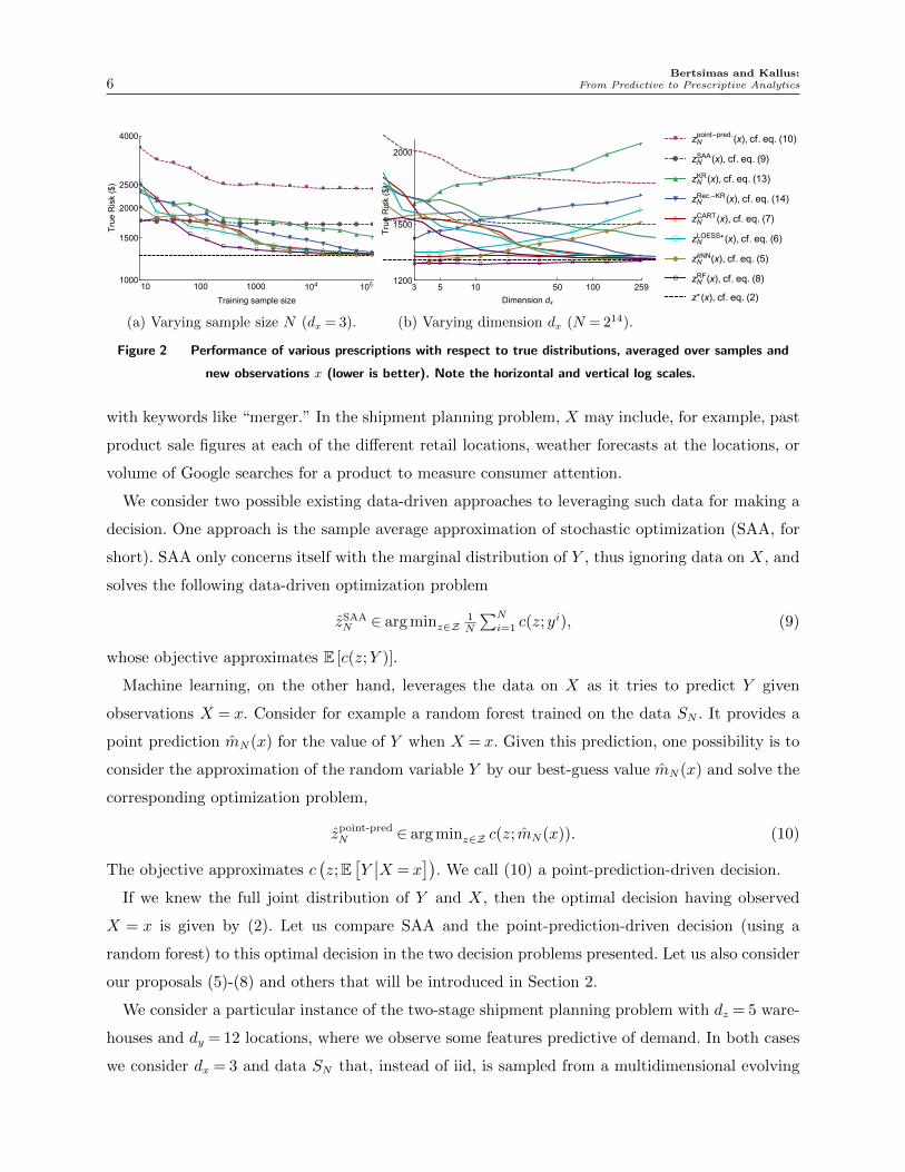
Figure 2 Performance of various prescriptions with respect to true distributions, averaged over samples and
new observations x (lower is better). Note the horizontal and vertical log scales.
with keywords like “merger.” In the shipment planning problem, X may include, for example, past
product sale figures at each of the di↵erent retail locations, weather forecasts at the locations, or
volume of Google searches for a product to measure consumer attention.
We consider two possible existing data-driven approaches to leveraging such data for making a
decision. One approach is the sample average approximation of stochastic optimization (SAA, for
short). SAA only concerns itself with the marginal distribution of Y , thus ignoring data on X, and
solves the following data-driven optimization problem
zSAAN 2 argminz2Z
1N
PN
i=1 c(z;yi), (9)
whose objective approximates E [c(z;Y )].
Machine learning, on the other hand, leverages the data on X as it tries to predict Y given
observations X = x. Consider for example a random forest trained on the data SN . It provides a
point prediction mN(x) for the value of Y when X = x. Given this prediction, one possibility is to
consider the approximation of the random variable Y by our best-guess value mN(x) and solve the
corresponding optimization problem,
zpoint-predN 2 argminz2Z c(z; mN(x)). (10)
The objective approximates c�z;E
⇥Y��X = x
⇤�. We call (10) a point-prediction-driven decision.
If we knew the full joint distribution of Y and X, then the optimal decision having observed
X = x is given by (2). Let us compare SAA and the point-prediction-driven decision (using a
random forest) to this optimal decision in the two decision problems presented. Let us also consider
our proposals (5)-(8) and others that will be introduced in Section 2.
We consider a particular instance of the two-stage shipment planning problem with dz = 5 ware-
houses and dy = 12 locations, where we observe some features predictive of demand. In both cases
we consider dx = 3 and data SN that, instead of iid, is sampled from a multidimensional evolving
Bertsimas and Kallus:From Predictive to Prescriptive Analytics 7
process in order to simulate real-world data collection. We give the particular parameters of the
problems in the supplementary Section 13. In Figure 2a, we report the average performance of the
various solutions with respect to the true distributions.
The full-information optimum clearly does the best with respect to the true distributions, as
expected. The SAA and point-prediction-driven decisions have performances that quickly converge
to suboptimal values. The former because it does not use observations on X and the latter because
it does not take into account the remaining uncertainty after observing X = x.1 In comparison,
we find that our proposals converge upon the full-information optimum given su�cient data. In
Section 4.3, we study the general asymptotics of our proposals and prove that the convergence
observed here empirically is generally guaranteed under only mild conditions.
Inspecting the figure further, it seems that ignoring X and using only the data on Y , as SAA does,
is appropriate when there is very little data; in both examples, SAA outperforms other data-driven
approaches for N smaller than ⇠64. Past that point, our constructions of predictive prescriptions,
in particular (5)-(8), leverage the auxiliary data e↵ectively and achieve better, and eventually
optimal, performance. The predictive prescription motivated by RF is notable in particular for
performing no worse than SAA in the small N regime, and better in the large N regime.
In this example, the dimension dx of the observations x was relatively small at dx = 3. In many
practical problems, this dimension may well be bigger, potentially inhibiting performance. E.g.,
in our real-world application in Section 6, we have dx = 91. To study the e↵ect of the dimension
of x on the performance of our proposals, we consider polluting x with additional dimensions of
uninformative components distributed as independent normals. The results, shown in Figure 2b,
show that while some of the predictive prescriptions show deteriorating performance with growing
dimension dx, the predictive prescriptions based on CART and RF are largely una↵ected, seemingly
able to detect the 3-dimensional subset of features that truly matter. In the supplemental Section
13.2 we also consider an alternative setting of this experiment where additional dimensions carry
marginal predictive power.
1.2. Relevant Literature
Stochastic optimization as in (1) has long been the focus of decision making under uncertainty in
OR/MS problems (cf. Birge and Louveaux (2011)) as has its multi-period generalization known
commonly as dynamic programming (cf. Bertsekas (1995)). The solution of stochastic optimization
problems as in (1) in the presence of data {y1, . . . , yN} on the quantity of interest is a topic of
active research. The traditional approach is the sample average approximation (SAA) where the
1 Note that the uncertainty of the point prediction in estimating the conditional expectation, gleaned e.g. via thebootstrap, is the wrong uncertainty to take into account, in particular because it shrinks to zero as N !1.

Bertsimas and Kallus:8 From Predictive to Prescriptive Analytics
true distribution is replaced by the empirical one (cf. Shapiro (2003), Shapiro and Nemirovski
(2005), Kleywegt et al. (2002)). Other approaches include stochastic approximation (cf. Robbins
and Monro (1951), Nemirovski et al. (2009)), robust SAA (cf. Bertsimas et al. (2014)), and data-
driven mean-variance distributionally-robust optimization (cf. Delage and Ye (2010), Calafiore
and El Ghaoui (2006)). A notable alternative approach to decision making under uncertainty in
OR/MS problems is robust optimization (cf. Ben-Tal et al. (2009), Bertsimas et al. (2011)) and
its data-driven variants (cf. Bertsimas et al. (2013), Calafiore and Campi (2005)). There is also a
vast literature on the tradeo↵ between the collection of data and optimization as informed by data
collected so far (cf. Robbins (1952), Lai and Robbins (1985), Besbes and Zeevi (2009)). In all of these
methods for data-driven decision making under uncertainty, the focus is on data in the assumed
form of iid observations of the parameter of interest Y . On the other hand, ML has attached great
importance to the problem of supervised learning wherein the conditional expectation (regression)
or mode (classification) of target quantities Y given auxiliary observations X = x is of interest (cf.
Trevor et al. (2001), Mohri et al. (2012)).
Statistical decision theory is generally concerned with the optimal selection of statistical estima-
tors (cf. Berger (1985), Lehmann and Casella (1998)). Following the early work of Wald (1949),
a loss function such as sum of squared errors or of absolute deviations is specified and the cor-
responding admissibility, minimax-optimality, or Bayes-optimality are of main interest. Statistical
decision theory and ML intersect most profoundly in the realm of regression via empirical risk
minimization (ERM), where a regression model is selected on the criterion of minimizing empirical
average of loss. A range of ML methods arise from ERM applied to certain function classes and
extensive theory on function-class complexity has been developed to analyze these (cf. Bartlett
and Mendelson (2003), Vapnik (2000, 1992)). Such ML methods include ordinary linear regression,
ridge regression, the LASSO of Tibshirani (1996), quantile regression, and `1-regularized quantile
regression of Belloni and Chernozhukov (2011). ERM is also closely connected with M -estimation
Geer (2000), which estimates a distributional parameter that maximizes an average of a function
of the parameter by the estimate that maximizes the corresponding empirical average. Unlike M -
estimation theory, which is concerned with estimation and inference, ERM theory is only concerned
with out-of-sample performance and can be applied more flexibly with less assumptions.
In certain OR/MS decision problems, one can employ ERM to select a decision policy, conceiving
of the loss as costs. Indeed, the loss function used in quantile regression is exactly equal to the cost
function of the newsvendor problem of inventory management. Rudin and Vahn (2014) consider
this loss function and the selection of a univariate-valued linear function with coe�cients restricted
in `1-norm in order to solve a newsvendor problem with auxiliary data, resulting in a method
similar to Belloni and Chernozhukov (2011). Kao et al. (2009) study finding a convex combination

Bertsimas and Kallus:From Predictive to Prescriptive Analytics 9
of two ERM solutions, the least-cost decision and the least-squares predictor, which they find
to be useful when costs are quadratic. In more general OR/MS problems where decisions are
constrained, we show in the supplemental Section 8 that ERM is not applicable. Even when it
is, a linear decision rule may be inappropriate as we show by example. For the limited problems
where ERM is applicable, we generalize the standard function-class complexity theory and out-of-
sample guarantees to multivariate decision rules since most OR/MS problems involve multivariate
decisions.
Instead of ERM, we are motivated more by a strain of non-parametric ML methods based on
local learning, where predictions are made based on the mean or mode of past observations that are
in some way similar to the one at hand. The most basic such method is kNN (cf. Altman (1992)),
which define the prediction as a locally constant function depending on which k data points lie
closest. A related method is Nadaraya-Watson kernel regression (KR) (cf. Nadaraya (1964), Watson
(1964)), which is notable for being highly amenable to theoretical analysis but sees less use in
practice. KR weighting for solving conditional stochastic optimization problems as in (2) has been
considered in Hanasusanto and Kuhn (2013), Hannah et al. (2010) but these have not considered
the more general connection to a great variety of ML methods used in practice and neither have they
considered asymptotic optimality rigorously. A more widely used local learning regression method
than KR is local regression (Cameron and Trivedi (2005) pg. 311) and in particular the LOESS
method of Cleveland and Devlin (1988). Even more widely used are recursive partitioning methods,
most often in the form of trees and most notably CART of Breiman et al. (1984). Ensembles of
trees, most notably RF of Breiman (2001), are known to be very flexible and have competitive
performance in a great range of prediction problems. The former averages locally over a partition
designed based on the data (the leaves of a tree) and the latter combines many such averages.
While there are many tree-based methods and ensemble methods, we focus on CART and RF
because of their popularity and e↵ectiveness in practice.
2. From Data to Predictive Prescriptions
Recall that we are interested in the conditional-stochastic optimization problem (2) of minimizing
uncertain costs c(z;Y ) after observing X = x. The key di�culty is that the true joint distribution
µX,Y , which specifies problem (2), is unknown and only data SN is available. One approach may
be to approximate µX,Y by the empirical distribution µN over the data SN where each datapoint
(xi, yi) is assigned mass 1/N . This, however, will in general fail unless X has small and finite
support; otherwise, either X = x has not been observed and the conditional expectation is undefined
with respect to µN or it has been observed, X = x = xi for some i, and the conditional distribution
is a degenerate distribution with a single atom at yi without any uncertainty. Therefore, we require

Bertsimas and Kallus:10 From Predictive to Prescriptive Analytics
some way to generalize the data to reasonably estimate the conditional expected costs for any x.
In some ways this is similar to, but more intricate than, the prediction problem where E[Y |X = x]
is estimated from data for any possible x 2 X . We are therefore motivated to consider predictive
methods and their adaptation to our cause.
In the next subsections we propose a selection of constructions of predictive prescriptions zN(x),
each motivated by a local-learning predictive methodology. All the constructions in this section will
take the common form of defining some data-driven weights wN,i(x) and optimizing the decision
zN against a re-weighting of the data, as in (3):
zlocalN (x)2 argminz2Z
PN
i=1 wN,i(x)c(z;yi). (11)
In some cases the weights are nonnegative and can be understood to correspond to an estimated
conditional distribution of Y given X = x. But, in other cases, some of the weights may be negative
and this interpretation breaks down.
2.1. kNN
Motivated by k-nearest-neighbor regression we propose
wkNNN,i (x) = 1
kI [xi is a kNN of x] , (12)
giving rise to the predictive prescription (5). Ties among equidistant data points are broken either
randomly or by a lower-index-first rule. Finding the kNNs of x without pre-computation can clearly
be done in O(Nd) time. Data-structures that speed up the process at query time at the cost of
pre-computation have been developed (cf. Bentley (1975)) and there are also approximate schemes
that can significantly speed up queries (c.f. Arya et al. (1998)).
2.2. Kernel Methods
The Nadaraya-Watson kernel regression (KR; cf. Nadaraya (1964), Watson (1964)) estimates
m(x) = E[Y |X = x] by
mN(x) =PN
i=1 yiK((xi�x)/hN)PN
i=1 K((xi�x)/hN),
where K : Rd !R, known as the kernel, satisfiesR
K <1 (and often unitary invariance) and hN >
0, known as the bandwidth. We restrict our attention to the following common kernels: K(x) =
I [||x|| 1] (Naıve), K(x) = (1�kxk2)I [kxk 1] (Epanechnikov), and K(x) = (1�kxk3)3I [kxk 1]
(Tri-cubic). For these (nonnegative) kernels, KR is the result of the conditional distribution estimate
that arises from the Parzen-window density estimates (cf. Parzen (1962)) of µX,Y and µX (i.e.,
their ratio). In particular, using the same conditional distribution estimate, the following weights
lead to a predictive prescription as in (3):
wKRN,i(x) =
K((xi�x)/hN)PN
j=1 K((xj�x)/hN). (13)

Bertsimas and Kallus:From Predictive to Prescriptive Analytics 11
Note that the naıve kernel with bandwidth hN corresponds directly to uniformly weighting all
neighbors of x that are within a radius hN .
A recursive modification to (13) that is motivated by an alternative kernel regressor introduced
by Devroye and Wagner (1980) is
wrecursive-KRN,i (x) =
K((xi�x)/hi)PN
j=1 K((xj�x)/hj), (14)
where now the bandwidths hi are selected per-data-point and independent of N . From a theoretical
point of view, much weaker conditions are necessary to ensure good asymptotic behavior of (14)
compared to (13), as we will see in the next section.
2.3. Local Linear Methods
Whereas KR estimates m(x) by the best local constant prediction weighted by the kernel (i.e.,
the weighted average), local linear regression estimates m(x) by the best local linear prediction
weighted by the kernel:
mN(x) = argmin�0min�1
PN
i=1 ki(x) (yi ��0 ��T1 (xi �x))
2.
In prediction, local linear methods are known to be preferable over KR (cf. Fan (1993)). Using this
to locally approximate the conditional costs E⇥c(z;Y )
��X = x⇤
by a linear function we will arrive
at a functional estimate and a predictive prescription as in (3) with the weights
wLOESSN,i (x) =
wN,i(x)PN
j=1 wN,j(x), wN,i(x) = ki(x)
⇣1�Pn
j=1 kj(x)(xj �x)T⌅(x)�1(xi �x)⌘
, (15)
where ⌅(x) =Pn
i=1 ki(x)(xi�x)(xi�x)T and ki(x) = K ((xi �x)/hN(x)). In LOESS regression per
(Cleveland and Devlin 1988), K is the tri-cubic kernel and hN(x) is the distance to x’s k-nearest
neighbor with k fixed. In Section 4.1, we establish the computational tractability of predictive
prescriptions as in (3) when weights are nonnegative. The weights (15), however, may sometimes be
negative. Nonetheless, as N increases, these weights will always become nonnegative. As such, we
propose a modification of weights (15) that ensures all weights are nonnegative without sacrificing
asymptotic optimality (see Section 4.3):
wLOESS*N,i (x) =
wN,i(x)PN
j=1 wN,j(x), wN,i(x) = ki(x)max{1�Pn
j=1 kj(x)(xj �x)T⌅(x)�1(xi �x),0}. (16)
2.4. Trees
In prediction, CART (Breiman et al. 1984) recursively splits the sample SN into regions in X along
axis-aligned cuts (one-hot hyperplanes) so to gain reduction in an impurity measure in the response
variable Y within each region. Common impurity measures are Gini or entropy for classification
and squared error for univariate regression. Multivariate impurity measures are the component-
wise average of univariate impurities. Once a tree is constructed, the value of m(x) is estimated
by the average of yi’s associated with the xi’s that reside in the same region as x.
Bertsimas and Kallus:12 From Predictive to Prescriptive Analytics
Regardless of the particular method chosen, a final partition can be represented as a binning
rule identifying points in X with the disjoint regions, R : X ! {1, . . . , r}. The partition is then
the disjoint union R�1(1)t · · ·tR�1(r) = X . The tree regression estimates correspond directly to
taking averages over the uniform distribution of the data points residing in the region R(x). For
our prescription problem, we propose to use the binning rule to construct weights as follows for a
predictive prescription of the form (3):
wCARTN,i (x) =
I[R(x)=R(xi)]|{j:R(xj)=R(x)}| . (17)
Notice that the weights (17) are piecewise constant over the partitions and therefore the rec-
ommended optimal decision zN(x) is also piecewise constant. Therefore, solving r optimization
problems after the recursive partitioning process, the resulting predictive prescription can be fully
compiled into a decision tree, with the decisions that are truly decisions. This also retains CART’s
lauded interpretability.2
2.5. Ensembles
A random forest (Breiman 2001) is an ensemble of trees each trained a random subsample of the
data with random subset of components of X considered at each tree node. After training such
a random forest of trees, we can extract the partition rules Rt t = 1, . . . , T , one for each tree in
the forest. We propose to use these to construct the following weights as follows for a predictive
prescription of the form (3):
wRFN,i(x) = 1
T
PT
t=1
I[Rt(x)=Rt(xi)]|{j:Rt(xj)=Rt(x)}| . (18)
In Section 1.1 we demonstrated that our predictive prescription based on RF, given in eq. (8),
performed well overall in two di↵erent problems, for a range of sample sizes, and for a range of
dimensions dx. Based on this evidence of flexible performance, we choose our predictive prescription
based on RF for our real-world application, which we study in Section 6.
3. From Data to Predictive Prescriptions When Decisions A↵ectUncertainty
Up to now, we have assumed that the e↵ect of the decision z on costs is wholly encapsulated in
the cost function and that the choice of z does not directly a↵ect the realization of uncertainty Y .
However, in some settings, such as in the presence of pricing decisions, this assumption clearly does
not hold – as one increases a price control, demand diminishes, and the causal e↵ect of pricing is not
2 A more direct application of tree methods to the prescription problem would have us consider the impurities beingminimized in each split to be equal to the mean cost c(z;y) of taking the best constant decision z in each side of thesplit. However, since we must consider splitting on each variable and at each data point to find the best split (cf. pg.307 of Trevor et al. (2001)), this can be overly computationally burdensome for all but the simplest problems thatadmit a closed form solution such as least sum of squares or the newsvendor problem.

Bertsimas and Kallus:From Predictive to Prescriptive Analytics 13
known a priori (e.g., can be abstracted in the cost function) and must be derived from data. In such
cases, we must take into account the e↵ect of our decision z on the uncertainty Y by considering
historical data {(x1, y1, z1), . . . , (xN , yN , zN)}, where we have also recorded historical observations
of the variable Z, which represents the historical decision taken in each instance. Using potential
outcomes, we let Y (z) denote the value of the uncertain variable that would be observed if decision
z were chosen. For each data point i, only the realization corresponding to the chosen decision zi
is revealed, yi = yi(zi). The counterfactual yi(z) that would have been observed under any other
decision z 6= zi is not available for measurement. (For detail on potential outcomes and history see
Imbens and Rubin 2015, Chapters 1-2.)
Since only some parts of our decision may have unknown e↵ects on uncertainty, we decompose
our decision variable into the part with unknown e↵ect (e.g., pricing decisions) and known e↵ect
(e.g., production decisions) in the following way:
Assumption 1 (Decomposition of Decision). For some decomposition z = (z1, z2) only z1 2Rdz1 a↵ects the uncertainty, i.e.,
Y (z1, z2) = Y (z1, z02) 8(z1, z2), (z1, z
02)2Z.
For brevity, we write Y (z) = Y (z1). And, we let Z1(z2) = {z1 : (z1, z2)2Z}, Z1 =
{z1 : 9z2 (z1, z2)2Z}, Z2(z1) = {z2 : (z1, z2)2Z}, Z2 = {z2 : 9z1 (z1, z2)2Z}.
For example, in pricing, if z1 2 [0,1) represents a price control for a product and Y represents
realized demand, then {(z1, Y (z1)) : z1 2 [0,1)} represents the random demand curve. If in the ith
data point the price was zi1, then we only observe the single point (zi
1, yi(zi
1)) on this random curve.
Decision components z2 could represent, for example, a production and shipment plan, which does
not a↵ect demand but does a↵ect final costs.
The immediate generalization of problem (2) to this setting is
v⇤(x) = minz2Z E⇥c(z;Y (z))
��X = x⇤, z⇤(x)2Z⇤(x) = argminz2Z E
⇥c(z;Y (z))
��X = x⇤. (19)
This problem depends on understanding the joint distribution of (X,Y (z)) for each z 2Z and, in
this full information setting, chooses z for least expected cost given the observation X = x and
the e↵ect z would have on the uncertainty Y (z). Assumption 1 allows problem (19) to encompass
the standard conditional stochastic optimization problem (2) by letting z = z2 and dz1= 0. On the
other hand, Assumption 1 is non-restrictive in the sense that it can be as general as necessary by
letting z = z1, i.e., no decomposing into parts of unknown e↵ect and known no e↵ect. For these
reason, we maintain the notation v⇤(x), z⇤(x), Z⇤(x).
Given only the data (xi, yi, zi) on (X,Y,Z) and without any assumptions, problem (19) is in
fact not well-specified because of the missing data on the counterfactuals. In particular, for any

Bertsimas and Kallus:14 From Predictive to Prescriptive Analytics
fixed joint distribution for (X,Y,Z), there are many possible distributions of (X,Y (z)) for each
z 2Z that all agree with the same distribution of (X,Y,Z) via the transformation Y = Y (Z) but
can each give rise to di↵erent optimal solutions z⇤(x) in (19) (see Bertsimas and Kallus 2016).
Therefore, problem (19) may not be solved using the data alone.
To eliminate this issue, we must make additional assumptions about the data. Here, we make
the assumption that controlling for X is su�cient for isolating the e↵ect of z on Y .
Assumption 2 (Ignorability). For every z 2Z, Y (z) is independent of Z conditioned on X.
In words, Assumption 2 says that, historically, X accounts for all the features associated with the
instance {Y (z) : z 2Z} that may have influenced managerial decision making. In the causal infer-
ence literature, this assumption is standard for ensuring identifiability of causal e↵ects (Rosenbaum
and Rubin 1983).
In stark contrast to many situations in causal inference dealing with latent self-selection, Assump-
tion 2 is particularly defensible in our specific setting. In the setting we consider, Z represents
historical managerial decisions and, just like future decisions to be made by the learned predictive
prescription, these decisions must have been made based on observable quantities available to the
manager. As long as these quantities were also recorded as part of X then Assumption 2 is guar-
anteed to hold. Alternatively, were decisions Z taken at random for exploration then Assumption
2 holds trivially.
3.1. Adapting local-learning methods
We now show how to generalize the predictive prescriptions from Section 2 to solve problem (19)
when decisions a↵ect uncertainty based on data on (X,Y,Z). We begin with a rephrasing of problem
(19) based on Assumptions 1 and 2. The proof is given in the E-companion.
Theorem 1. Under Assumptions 1 and 2, problem (19) is equivalent to,
min(z1,z2)2Z E⇥c(z;Y )
��X = x, Z1 = z1
⇤. (20)
Note that problem (20) depends only on the distribution of the data (X, Y, Z), does not involve
unknown counterfactuals, and has the form of a conditional stochastic optimization problem. Cor-
respondingly, all predictive-prescriptive local-learning methods from Section 2 can be adapted to
this problem by simply augmenting the data xi with zi1. In particular, we can consider data-driven
predictive prescriptions of the form
zN(x)2 argminz2ZPN
i=1 wN,i(x, z1)c(z;yi), (21)
where wN,i(x, z1) are weight functions derived from the data by simply taking the same approach
as in Section 2 but treating z1 as part of the X data. In particular, for each method in Section
Bertsimas and Kallus:From Predictive to Prescriptive Analytics 15
2, we let xi = (xi, zi1), construct weights wN,i(x) based on data SN = {(x1, y1), . . . , (xN , yN)}, and
plug wN,i(x) into (21), and compute zN(x). For example, the kNN approach applied to (19) has
the form (21) with weights
wkNNN,i (x, z1) = 1
kI [(xi, zi
1) is a kNN of (x, z1)] .
As we discuss in Section 4.2, there is an increased computational burden in solving problem (21)
when decisions a↵ect uncertainty, compared to our standard predictive prescriptions from Section
2. As we show in Section 4.4, this approach produces prescriptions that are asymptotically optimal
even when our decisions have an unknown e↵ect on uncertainty.
3.2. Example: two-stage shipment planning with pricing
Consider a pricing variation on our two-stage shipment planning problem from Section 1.1. We
introduce an additional decision variable z1 2 [0,1) for the price at which we sell the product.
The uncertain demand at the dy locations Y (z1) depends on the price we set. In the first stage,
we determine price z1 and amounts z2 at dz2warehouses. In the second stage, instead of shipping
from warehouses to satisfy all demand, we can ship as much as we would like. Our profit is the
price times number of units sold minus production and transportation costs. Assuming we behave
optimally in the second stage, we can write the problem using the cost function and feasible set
c(z;y) = p1
Pdz2i=1 z2,i + min
(t,s)2Q(z,y)(p2
Pdz2i=1 ti +
Pdz2i=1
Pdy
j=1(cij � z1)sij),
Z =�(z1, z2)2R1+dz2 : z1, z2 � 0
,
where Q(z, y) = {(s, t)2R(dz⇥dy)⇥dz : t� 0, s� 0,Pdz
i=1 sij yj 8j,Pdy
j=1 sij z2,i + ti 8i}.We now consider observing not only X and Y but also Z1. We consider the same parameters
of the problem as in Section 1.1 with an added unknown e↵ect of price on demand so that higher
prices induce lower demands. The particular parameters are given in the supplementary Section 13.
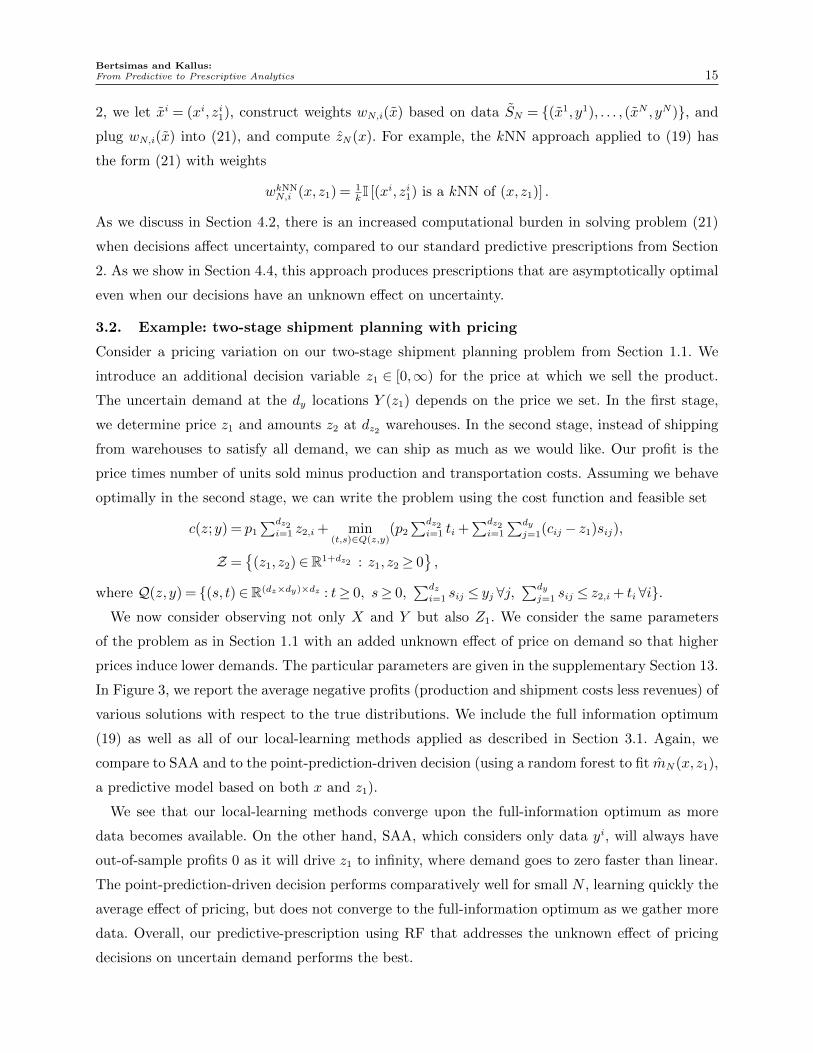
In Figure 3, we report the average negative profits (production and shipment costs less revenues) of
various solutions with respect to the true distributions. We include the full information optimum
(19) as well as all of our local-learning methods applied as described in Section 3.1. Again, we
compare to SAA and to the point-prediction-driven decision (using a random forest to fit mN(x, z1),
a predictive model based on both x and z1).
We see that our local-learning methods converge upon the full-information optimum as more
data becomes available. On the other hand, SAA, which considers only data yi, will always have
out-of-sample profits 0 as it will drive z1 to infinity, where demand goes to zero faster than linear.
The point-prediction-driven decision performs comparatively well for small N , learning quickly the
average e↵ect of pricing, but does not converge to the full-information optimum as we gather more
data. Overall, our predictive-prescription using RF that addresses the unknown e↵ect of pricing
decisions on uncertain demand performs the best.
Bertsimas and Kallus:16 From Predictive to Prescriptive Analytics
● ● ● ● ● ● ● ● ● ● ● ●▲ ▲ ▲ ▲ ▲
▲ ▲▲
▲▲
▲▲
■
■■ ■
■■ ■ ■ ■ ■ ■ ■
▼ ▼ ▼ ▼ ▼
▼▼
▼ ▼▼
▼
▼
◆◆ ◆ ◆
◆
◆
◆◆ ◆ ◆ ◆ ◆
○
○
○
○ ○
○○
○ ○ ○ ○ ○
◇ ◇
◇ ◇◇ ◇
◇◇ ◇ ◇ ◇
◇
□
□
□□ □
□□
□ □ □ □ □10 50 100 500 1000 5000 104
-3000
-2500
-2000
-1500
-1000
-500
0
Training sample size
TrueRisk($)
● zNSAA(x), cf. eq. (9)
▲ zNKR(x), cf. eq. (13)
■ zNpoint-pred.(x), cf. eq. (10)
▼ zNRec.-KR(x), cf. eq. (14)
◆ zNkNN(x), cf. eq. (5)
○ zNLOESS*(x), cf. eq. (6)
◇ zNCART(x), cf. eq. (7)
□ zNRF(x), cf. eq. (8)
z*(x), cf. eq. (2)
Figure 3 Performance of various prescriptions in the two-stage shipment planning with pricing problem.
4. Properties of Local Predictive Prescriptions
In this section, we study two important properties of local predictive prescriptions: computational
tractability and asymptotic optimality. All proofs are given in the E-companion.
4.1. Tractability
In Section 2, we considered a variety of predictive prescriptions zN(x) that are computed by solving
the optimization problem (3). An important question is then when is this optimization problem
computationally tractable to solve. As an optimization problem, problem (3) di↵ers from the prob-
lem solved by the standard SAA approach (9) only in the weights given to di↵erent observations.
Therefore, it is similar in its computational complexity and we can defer to computational studies
of SAA such as Shapiro and Nemirovski (2005) to study the complexity of solving problem (3). For
completeness, we develop su�cient conditions for problem (3) to be solvable in polynomial time.
Theorem 2. Fix x and weights wN,i(x)� 0. Suppose Z is a closed convex set and let a separation
oracle for it be given. Suppose also that c(z;y) is convex in z for every fixed y and let oracles be
given for evaluation and subgradient in z. Then for any x we can find an ✏-optimal solution to (3)
in time and oracle calls polynomial in N0, d, log(1/✏) where N0 =PN
i=1 I [wN,i(x) > 0] N is the
e↵ective sample size.
Note that all of weights presented in Section 2 are all nonnegative with the exception of local
regression (15), which is what led us to their nonnegative modification (16).
4.2. Tractability When Decisions A↵ect Uncertainty
Solving problem (21) with general weights wiN(x, z1) is generally hard as the objective of problem
(21) may be non-convex in z. In some specific instances we can maintain tractability, while in
others we can devise specialized approaches that allow us to solve problem (21) in practice.
In the simplest case, if Z1 = {z11, . . . , z1b} is discrete then the problem can simply be solved by
optimizing once for each fixed value of z1, letting z2 remain variable.

Bertsimas and Kallus:From Predictive to Prescriptive Analytics 17
Theorem 3. Fix x and weights wN,i(x, z1)� 0. Suppose Z1 = {z11, . . . , z1b} is discrete and that
Z2(z1j) is a closed convex set for each j = 1, . . . , b and let a separation oracle for it be given. Suppose
also that c((z1, z2);y) is convex in z2 for every fixed y, z1 and let oracles be given for evaluation and
subgradient in z2. Then for any x we can find an ✏-optimal solution to (21) in time and oracle calls
polynomial in N0, b, d, log(1/✏) where N0 =PN
i=1 I [wN,i(x) > 0]N is the e↵ective sample size.
Note that the convexity in z2 condition is weaker than convexity in z, which would be su�cient.
Alternatively, if Z1 is not discrete, we can approach the problem using discretization, which leads
to exponential dependence in z1’s dimension dz1and the precision log(1/✏).
Theorem 4. Fix x and weights wN,i(x, z1) � 0. Suppose c((z1, z2);y) is L-Lipschitz in z1 for
each z2 2 Z2, that Z1 is bounded, and that Z2(z1) is a closed convex set for each z1 2 Z1 and let
a separation oracle for it be given. Suppose also that c((z1, z2);y) is convex in z2 for every fixed
y, z1 and let oracles be given for evaluation and subgradient in z2. Then for any x we can find an
✏-optimal solution to (21) in time and oracle calls polynomial in N0, b, d, log(1/✏), (L/✏)dz1 where
N0 =PN
i=1 I [wN,i(x) > 0]N is the e↵ective sample size.
Although the exponential dependence in dz1and super-logarithmic dependence in 1/✏ appears
problematic, this approach works well in practice only for small dz1. For example, we use this
approach in our pricing example in Section 3.2, where dz1= 1, to successfully solve many instances
of (21).
For the specific case of tree weights, we can discretize the problem exactly, leading to a particu-
larly e�cient algorithm in practice. Suppose we are given the CART partition rule R : X ⇥Z1 !{1, . . . , r}, then we can solve problem (21) exactly as follows:
1. Let x be given and fix wCARTN,i (x, z1) =
I[R(x,z1)=R(xi,zi1)]
|{j:R(xj ,zj1)=R(x,z1)}|
.
2. Find the partitions that contain x, J = {j : 9z1, (x, z1)2R�1(j)}, and compute the constraints
on z1 in each part, Z1j =�z1 : 9x, (x, z1)2R(�1)(j)
for j 2 J . This is easily done by going
down the tree and at each node, if the node queries the value of x we only take the branch
that corresponds to the value of our given x and if the node queries the value of a component
of z1 then we take both branches and record the constraint on z1 on each side.
3. For each j 2J , solve
vj = minz2Z:z2Z1j
Pi:R(xi,zi
1)=j c(z;yi), zj = argminz2Z:z2Z1j
Pi:R(xi,zi
1)=j c(z;yi).
(These can be solved for in advance for each j = 1, . . . , r to reduce computation at query time.)
4. Let j(x) = argminj2J vj and zn(x) = zj(x).
This procedure solves (21) exactly for weights wCARTN,i (x, z1).
Bertsimas and Kallus:18 From Predictive to Prescriptive Analytics
4.3. Asymptotic Optimality
In Section 1.1, we saw that our predictive prescriptions zN(x) converged to the full-information
optimum as the sample size N grew. Next, we show that this anecdotal evidence is supported
by mathematics and that such convergence is guaranteed under only mild conditions. We define
asymptotic optimality as the desirable asymptotic behavior for zN(x).
Definition 1. We say that zN(x) is asymptotically optimal if, with probability 1, we have that
for µX-almost-everywhere x2X ,
limN!1 E⇥c(zN(x);Y )
��X = x⇤= v⇤(x).
We say zN(x) is consistent if, with probability 1, we have that for µX-almost-everywhere x2X ,
limN!1
||zN(x)�Z⇤(x)|| = 0, where ||zN(x)�Z⇤(x)|| = infz2Z⇤(x)
||zN(x)� z|| .
To a decision maker, asymptotic optimality is the most critical limiting property as it says that
decisions implemented will have performance reaching the best possible. Consistency refers to the
consistency of zN(x) as a statistical estimator for the full-information optimizer(s) Z⇤(x) and is
perhaps less critical for a decision maker but will be shown to hold nonetheless.
Asymptotic optimality and depends on our choice of zN(x), the structure of the decision problem
(cost function and feasible set), and on how we accumulate our data SN . The traditional assumption
on data collection is that it constitutes an iid process. This is a strong assumption and is often
only a modeling approximation. The velocity and variety of modern data collection often means
that historical observations do not generally constitute an iid sample in any real-world application.
We are therefore motivated to consider an alternative model for data collection, that of mixing
processes. These encompass such processes as ARMA, GARCH, and Markov chains, which can
correspond to sampling from evolving systems like prices in a market, daily product demands, or
the volume of Google searches on a topic. While many of our results extend to such settings via
generalized strong laws of large numbers (Walk 2010), we present only the iid case in the main
text to avoid cumbersome exposition and defer these extensions to the supplemental Section 9.2.
For the rest of the section let us assume that SN is generated by iid sampling.
As mentioned, asymptotic optimality also depends on the structure of the decision problem.
Therefore, we will also require the following conditions.
Assumption 3 (Existence). The full-information problem (2) is well defined: E [|c(z;Y )|] <1for every z 2Z and Z⇤(x) 6=? for almost every x.
Assumption 4 (Continuity). c(z;y) is equicontinuous in z: for any z 2 Z and ✏ > 0 there
exists � > 0 such that |c(z;y)� c(z0;y)| ✏ for all z0 with ||z � z0|| � and y 2Y.
Assumption 5 (Regularity). Z is closed and nonempty and in addition either

Bertsimas and Kallus:From Predictive to Prescriptive Analytics 19
1. Z is bounded or
2. lim inf ||z||!1 infy2Y c(z;y) > �1 and for every x 2 X , there exists Dx ⇢ Y such that
lim||z||!1 c(z;y)!1 uniformly over y 2Dx and P�y 2Dx
��X = x�> 0.
Under these conditions, we have the following su�cient conditions for asymptotic optimality,
which are proven as consequences of universal pointwise convergence results of related supervised
learning problem of Walk (2010), Hansen (2008).
Theorem 5 (kNN). Suppose Assumptions 3, 4, and 5 hold. Let wN,i(x) be as in (12) with k =
min�dCN �e,N � 1
for some C > 0, 0 < � < 1. Let zN(x) be as in (3). Then zN(x) is asymptotically
optimal and consistent.
Theorem 6 (Kernel Methods). Suppose Assumptions 3, 4, and 5 hold and that
E [|c(z;Y )|max{log |c(z;Y )| ,0}] < 1 for each z. Let wN,i(x) be as in (13) with K being any of
the kernels in Section 2.2 and hN = CN�� for C > 0, 0 < � < 1/dx. Let zN(x) be as in (3). Then
zN(x) is asymptotically optimal and consistent.
Theorem 7 (Recursive Kernel Methods). Suppose Assumptions 3, 4, and 5 hold. Let
wN,i(x) be as in (14) with K being the naıve kernel and hi = Ci�� for some C > 0, 0 < � < 1/(2dx).
Let zN(x) be as in (3). Then zN(x) is asymptotically optimal and consistent.
Theorem 8 (Local Linear Methods). Suppose Assumptions 3, 4, and 5 hold, that µX is
absolutely continuous and has density bounded away from 0 and 1 on the support of X and twice
continuously di↵erentiable, and that costs are bounded over y for each z (i.e., |c(z;y)| g(z)) and
twice continuously di↵erentiable. Let wN,i(x) be as in (15) with K being any of the kernels in
Section 2.2 and with hN = CN�� for some C > 0, 0 < � < 1/dx. Let zN(x) be as in (3). Then zN(x)
is asymptotically optimal and consistent.
Theorem 9 (Nonnegative Local Linear Methods). Suppose Assumptions 3, 4, and 5 hold,
that µX is absolutely continuous and has density bounded away from 0 and 1 on the support
of X and twice continuously di↵erentiable, and that costs are bounded over y for each z (i.e.,
|c(z;y)| g(z)) and twice continuously di↵erentiable. Let wN,i(x) be as in (16) with K being any
of the kernels in Section 2.2 and with hN = CN�� for some C > 0, 0 < � < 1/dx. Let zN(x) be as
in (3). Then zN(x) is asymptotically optimal and consistent.
Although we do not have firm theoretical results on the asymptotic optimality of the predictive
prescriptions based on CART (eq. (7)) and RF (eq. (8)), we have observed them to converge
empirically in Section 1.1.
Bertsimas and Kallus:20 From Predictive to Prescriptive Analytics
4.4. Asymptotic Optimality When Decisions A↵ect Uncertainty
When decisions a↵ect uncertainty, the condition for asymptotic optimality is subtly di↵erent. Under
the identity Y = Y (Z), Definiton 1 does not accurately reflect asymptotic optimality and indeed
methods that do not account for the unknown e↵ect of the decision (e.g., if we apply our methods
without regard to this e↵ect, ignoring data on Z1) will not reach the full-information optimum
given by (19). Instead, we would like to ensure that our decisions have optimal cost when taking
into account their e↵ect on uncertainty. The desired asymptotic behavior for zN(x) when decisions
a↵ect uncertainty is the more general condition given below.
Definition 2. We say that zN(x) is asymptotically optimal if, with probability 1, we have that
for µX-almost-everywhere x2X , as N !1
limN!1 E⇥c(zN(x);Y (zN(x)))
��X = x⇤= minz2Z E
⇥c(z;Y (z))
��X = x⇤.
The following theorem establishes asymptotic optimality for our predictive prescription based
on either kernel methods, local linear methods, or nonnegative local linear methods as adapted
to the case when decisions a↵ect uncertainty. As in Section 3.1, we use xi to denote (xi, zi1) and
SN = {(x1, y1), . . . , (xN , yN)}. To avoid issues of existence, we focus on weak minimizers zN(x) of
(21) and on asymptotic optimality.
Theorem 10. Suppose Assumptions 1, 2, 3, 4, and 5 (case 1) hold, that µ(X,Z1) is absolutely
continuous and has density bounded away from 0 and 1 on the support of X,Z1 and twice contin-
uously di↵erentiable, and that costs are bounded over y for each z (i.e., |c(z;y)| g(z)) and twice
continuously di↵erentiable. Let wN,i(x) be as in (13), (15), or (16) applied to SN with K being any
of the kernels in Section 2.2 and with hN = CN�� for some C > 0, 0 < � < 1/(dx + dz1). Then for
any ✏N ! 0, any zN(x) that ✏N -minimizes (21) (has objective value within ✏N of the infimum) is
asymptotically optimal.
5. Metrics of Prescriptiveness
In this section, we develop a relative, unitless measure of the e�cacy of a predictive prescription.
An absolute measure of e�cacy is marginal expected costs,
R(zN) = E⇥E⇥c (zN(X);Y )
��X⇤⇤
= E [c (zN(X);Y )] .
Given a validation data set SNv = ((x1, y1), · · · , (xNv , yNv)), we estimate R(zN) as
RNv(zN) = 1Nv
PNv
i=1 c (zN(xi); yi) .
If SNv is disjoint and independent of the training set SN , then this is an out-of-sample estimate
that provides an unbiased estimate of R(zN). While an absolute measure allows one to compare two
predictive prescriptions for the same problem and data, a relative measure can quantify the overall
Bertsimas and Kallus:From Predictive to Prescriptive Analytics 21
□
□
□□ □ □ □ □ □ □ □ □ □
◆◆
◆ ◆
◆
◆◆
◆ ◆ ◆ ◆ ◆ ◆
○
○○ ○
○
○ ○○ ○ ○ ○ ○ ○
◇ ◇◇ ◇
◇
◇ ◇ ◇ ◇ ◇ ◇ ◇ ◇
▼
▼ ▼
▼ ▼▼
▼▼
▼▼
▼▼ ▼
▲▲
▲
▲ ▲ ▲ ▲ ▲▲ ▲ ▲
▲ ▲
● ● ● ● ● ● ● ● ● ● ● ● ●
100 1000 10000 100000
-0.2
0.0
0.2
0.4
Training sample size
CoefficientofPrescriptivenessP
(a) Varying sample size N .
□ □ □ □ □ □ □ □ □ □ □□□□□□□ □ □ □
□
◆ ◆ ◆ ◆ ◆ ◆ ◆◆◆◆◆◆◆◆◆◆◆◆◆◆
◆
◇ ◇ ◇ ◇ ◇ ◇ ◇ ◇ ◇ ◇ ◇◇◇◇◇◇◇ ◇ ◇ ◇
◇
○ ○ ○ ○ ○ ○ ○ ○○○○○○○○○○○○○
○
▼ ▼ ▼ ▼ ▼ ▼ ▼ ▼▼ ▼ ▼▼▼
▼▼▼▼ ▼ ▼ ▼
▼
▲ ▲ ▲ ▲ ▲▲ ▲ ▲
▲ ▲ ▲▲▲▲▲
▲▲ ▲ ▲ ▲
▲
■■■■■
■■■■■■
■
□ □ □ □ □ □ □ □ □ □ □□□□□□□ □ □ □
□
● ● ● ● ● ● ● ● ● ●●●●●●● ● ● ● ●
0.005 0.010 0.050 0.100 0.500 1-1.0
-0.5
0.0
0.5
1.0
Average coefficient of determination R2
CoefficientofPrescriptivenessP
(b) Varying determination R2
(N = 214).
z*(x), cf. eq. (2)
□ zNRF(x), cf. eq. (8)
◆ zNkNN(x), cf. eq. (5)
◇ zNCART(x), cf. eq. (7)
○ zNLOESS*(x), cf. eq. (6)
▼ zNRec.-KR(x), cf. eq. (14)
▲ zNKR(x), cf. eq. (13)
■ zNpoint-pred.(x), cf. eq. (10)
□ zNRF(x), cf. eq. (8)
● zNSAA(x), cf. eq. (9)
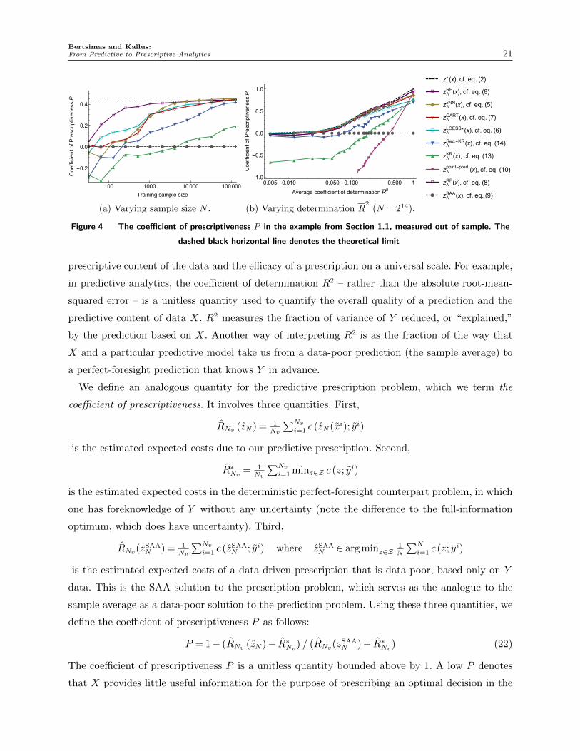
Figure 4 The coe�cient of prescriptiveness P in the example from Section 1.1, measured out of sample. The
dashed black horizontal line denotes the theoretical limit
prescriptive content of the data and the e�cacy of a prescription on a universal scale. For example,
in predictive analytics, the coe�cient of determination R2 – rather than the absolute root-mean-
squared error – is a unitless quantity used to quantify the overall quality of a prediction and the
predictive content of data X. R2 measures the fraction of variance of Y reduced, or “explained,”
by the prediction based on X. Another way of interpreting R2 is as the fraction of the way that
X and a particular predictive model take us from a data-poor prediction (the sample average) to
a perfect-foresight prediction that knows Y in advance.
We define an analogous quantity for the predictive prescription problem, which we term the
coe�cient of prescriptiveness. It involves three quantities. First,
RNv (zN) = 1Nv
PNv
i=1 c (zN(xi); yi)
is the estimated expected costs due to our predictive prescription. Second,
R⇤Nv
= 1Nv
PNv
i=1 minz2Z c (z; yi)
is the estimated expected costs in the deterministic perfect-foresight counterpart problem, in which
one has foreknowledge of Y without any uncertainty (note the di↵erence to the full-information
optimum, which does have uncertainty). Third,
RNv(zSAAN ) = 1
Nv
PNv
i=1 c (zSAAN ; yi) where zSAA
N 2 argminz2Z1N
PN
i=1 c (z;yi)
is the estimated expected costs of a data-driven prescription that is data poor, based only on Y
data. This is the SAA solution to the prescription problem, which serves as the analogue to the
sample average as a data-poor solution to the prediction problem. Using these three quantities, we
define the coe�cient of prescriptiveness P as follows:
P = 1� (RNv (zN)� R⇤Nv
) / (RNv(zSAAN )� R⇤
Nv) (22)
The coe�cient of prescriptiveness P is a unitless quantity bounded above by 1. A low P denotes
that X provides little useful information for the purpose of prescribing an optimal decision in the

Bertsimas and Kallus:22 From Predictive to Prescriptive Analytics
particular problem at hand or that zN(x) is ine↵ective in leveraging the information in X. A high
P denotes that taking X into consideration has a significant impact on reducing costs and that zN
is e↵ective in leveraging X for this purpose.
In particular, if X is independent of Y then, under appropriate conditions,
limN,Nv!1 RNv(zSAAN ) = minz2Z E [c(z;Y )] = E
⇥minz2Z E
⇥c(z;Y )
��X⇤⇤
= limN,Nv!1 RNv(zN), so
as N grows, we would see P reach 0. On the other hand, if Y is measurable with respect
to X, i.e., Y is a function of X, then, under appropriate conditions, limN,Nv!1 RNv(zN) =
E⇥minz2Z E
⇥c(z;Y )
��X⇤⇤
= E [minz2Z c(z;Y )] = limNv!1 R⇤Nv
, so as N grows, we would see P
reach 1. It is also notable that in the extreme case that Y is function of X then Y = m(X) where
m(x) = E⇥Y��X = x
⇤so that E [minz2Z c(z;Y )] = E [minz2Z c(z;m(X))], and so in this extreme
case we would see P reach 1 for zpoint-predN under appropriate conditions. In the independent case,
we would always see P reach a nonpositive number under zpoint-predN .
Let us consider the coe�cient of prescriptiveness in the example from Section 1.1. For each of
our predictive prescriptions and for each N , we measure the out of sample P on a validation set
of size Nv = 200 and plot the results in Figure 4a. Notice that even when we converge to the full-
information optimum, P does not approach 1 as N grows. Instead we see that for the same methods
that converged to the full-information optimum, we have a P that approaches 0.46. This number
represents the extent of the potential that X has to reduce costs in this particular problem. It is
the fraction of the way that knowledge of X, leveraged correctly, takes us from making a decision
under full uncertainty about the value of Y to making a decision in a completely deterministic
setting. As is the case with R2, what magnitude of P denotes a successful application depends on
the context. In our real-world application in Section 6, we find an out-of-sample P of 0.88.
To consider the relationship between how predictive X is of Y and the coe�cient of prescrip-
tiveness, we consider modifying the example by varying the magnitude of residual noise, fixing
N = 214. The details are given in the supplementary Section 13. As we vary the noise, we can vary
the average coe�cient of determination,
R2= 1� 1
dy
Pdy
i=1E[Var(Yi|X)]
Var(Yi),
from 0 to 1. In the original example, R2= 0.16. We plot the results in Figure 4b, noting that the
behavior matches our description of the extremes above. In particular, when X and Y are inde-
pendent (R2= 0), we see most methods having a zero coe�cient of prescriptiveness, less successful
methods (KR) have a somewhat negative coe�cient, and the point-prediction-driven decision has
a very negative coe�cient. When Y is measurable with respect to X (R2= 1), the coe�cient of the
optimal decision reaches 1, most methods have a coe�cient near 1, and the point-prediction-driven

Bertsimas and Kallus:From Predictive to Prescriptive Analytics 23
decision also has a coe�cient near 1 and beats most other methods. While neither extreme is rea-
sonable in practice, throughout the range, the predictive prescription motivated by RF performs
particularly well.
6. A Real-World Application
In this section, we apply our approach to a real-world problem faced by the distribution arm of
an international media conglomerate (the vendor) and demonstrate that our approach, combined
with extensive data collection, leads to significant advantages. The vendor has asked us to keep its
identity confidential as well as data on sale figures and specific retail locations. Some figures are
therefore shown on relative scales.
6.1. Problem Statement
The vendor sells over 0.5 million entertainment media titles on CD, DVD, and BluRay at over
50,000 retailers across the US and Europe. On average they ship 1 billion units in a year. The
retailers range from electronic home goods stores to supermarkets, gas stations, and convenience
stores. These have vendor-managed inventory (VMI) and scan-based trading (SBT) agreements
with the vendor. VMI means that the inventory is managed by the vendor, including replenishment
(which they perform weekly) and planogramming. SBT means that the vendor owns all inventory
until sold to the consumer, at which point the retailer buys the unit from the vendor and sells it to
the consumer. This means that retailers have no cost of capital in holding the vendor’s inventory.
The cost of a unit of entertainment media consists mainly of the cost of production of the
content. Media-manufacturing and delivery costs are secondary in e↵ect. Therefore, the primary
objective of the vendor is simply to sell as many units as possible and the main limiting factor is
inventory capacity at the retail locations. For example, at many of these locations, shelf space for
the vendor’s entertainment media is limited to an aisle endcap display and no back-of-the-store
storage is available. Thus, the main loss incurred in over-stocking a particular product lies in the
loss of potential sales of another product that sold out but could have sold more. In studying this
problem, we will restrict our attention to the replenishment and sale of video media only and to
retailers in Europe.
Apart from the limited shelf space the other main reason for the di�culty of the problem is the
particularly high uncertainty inherent in the initial demand for new releases. Whereas items that
have been sold for at least one period have a somewhat predictable decay in demand, determining
where demand for a new release will start is a much less trivial task. At the same time, new releases
present the greatest opportunity for high demand and many sales.
We now formulate the full-information problem. Let r = 1, . . . , R index the locations, t = 1, . . . , T
index the replenishment periods, and j = 1, . . . , d index the products. Denote by zj the order
Bertsimas and Kallus:24 From Predictive to Prescriptive Analytics
quantity decision for product j, by Yj the uncertain demand for product j, and by Kr the over-
all inventory capacity at location r. Considering only the main e↵ects on revenues and costs as
discussed in the previous paragraph, the problem decomposes on a per-replenishment-period, per-
location basis. We therefore wish to solve, for each t and r, the following problem:
v⇤(xtr) = max E
"Pd
j=1 min{Yj, zj}�����X = xtr
#=Pd
j=1 E⇥min{Yj, zj}
��Xj = xtr
⇤(23)
s.t. z � 0,Pd
j=1 zj Kr,
where xtr denotes auxiliary data available at the beginning of period t in the (t, r)th problem.
Note that had there been no capacity constraint in problem (23) and a per-unit ordering cost
were added, the problem would decompose into d separate newsvendor problems, the solution to
each being exactly a quantile regression on the regressors xtr. As it is, the problem is coupled, but,
fixing xtr, the capacity constraint can be replaced with an equivalent per-unit ordering cost � via
Lagrangian duality and the optimal solution is attained by setting each zj to the �th conditional
quantile of Yj. However, the reduction to quantile regression does not hold since the dual optimal
value of � depends simultaneously on all of the conditional distributions of Yj for j = 1, . . . , d.
6.2. Applying Predictive Prescriptions to Censored Data
In applying our approach to problem (23), we face the issue that we have data on sales, not demand.
That is, our data on the quantity of interest Y is right-censored. In this section, we develop a
modification of our approach to correct for this. The results in this section apply generally.
Suppose that instead of data {y1, . . . , yN} on Y , we have data {u1, . . . , uN} on U = min{Y, V }where V is an observable random threshold, data on which we summarize via � = I [U < V ]. For
example, in our application, V is the on-hand inventory level at the beginning of the period. Overall,
our data consists of SN = {(x1, u1, �1), . . . , (xN , uN , �N)}.One way to deal with this is by considering decisions (sock levels) as a↵ecting uncertainty (sales).
As long as demand and threshold are conditionally independent given X, Assumption 2 will be
satisfied and we can use the approach (21) developed in Section 3.1. However, the particular setting
of censored data has a lot structure where we actually know the mechanism of how decision a↵ect
uncertainty. This allows us to develop a special-purpose solution that side-steps the need to learn
the structure of this dependence and computationally less tractable approaches (Section 4.2).
In order to correct for the fact that our observations are in fact censored, we develop a conditional
variant of the Kaplan-Meier method (cf. Kaplan and Meier (1958), Huh et al. (2011)) to transform
our weights appropriately. Let (i) denote the ordering u(1) · · · u(N). Given the weights wN,i(x)
generated based on the naıve assumption that yi = ui, we transform these into the weights
wKaplan-MeierN,(i) (x) = I
⇥�(i) = 1
⇤✓ wN,(i)(x)PN
`=i wN,(`)(x)
◆Qki�1 : �(k)=1
✓PN`=k+1 wN,(`)(x)
PN`=k wN,(`)(x)
◆. (24)
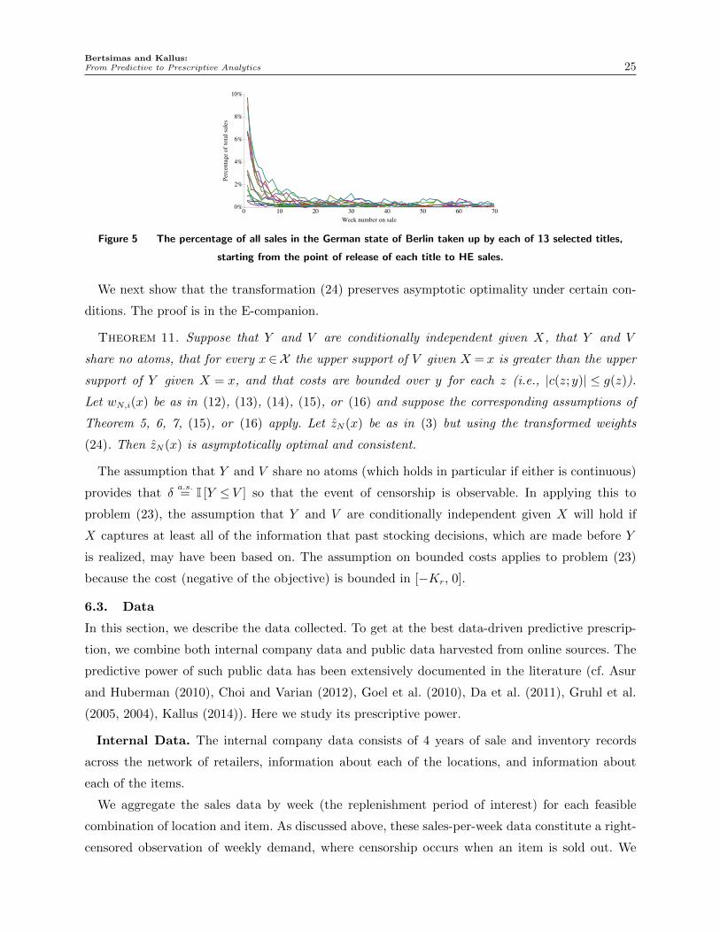
Bertsimas and Kallus:From Predictive to Prescriptive Analytics 25
0 10 20 30 40 50 60 700%
2%
4%
6%
8%
10%
Week number on salePercentageoftotalsales
Figure 5 The percentage of all sales in the German state of Berlin taken up by each of 13 selected titles,
starting from the point of release of each title to HE sales.
We next show that the transformation (24) preserves asymptotic optimality under certain con-
ditions. The proof is in the E-companion.
Theorem 11. Suppose that Y and V are conditionally independent given X, that Y and V
share no atoms, that for every x2X the upper support of V given X = x is greater than the upper
support of Y given X = x, and that costs are bounded over y for each z (i.e., |c(z;y)| g(z)).
Let wN,i(x) be as in (12), (13), (14), (15), or (16) and suppose the corresponding assumptions of
Theorem 5, 6, 7, (15), or (16) apply. Let zN(x) be as in (3) but using the transformed weights
(24). Then zN(x) is asymptotically optimal and consistent.
The assumption that Y and V share no atoms (which holds in particular if either is continuous)
provides that �a.s.= I [Y V ] so that the event of censorship is observable. In applying this to
problem (23), the assumption that Y and V are conditionally independent given X will hold if
X captures at least all of the information that past stocking decisions, which are made before Y
is realized, may have been based on. The assumption on bounded costs applies to problem (23)
because the cost (negative of the objective) is bounded in [�Kr, 0].
6.3. Data
In this section, we describe the data collected. To get at the best data-driven predictive prescrip-
tion, we combine both internal company data and public data harvested from online sources. The
predictive power of such public data has been extensively documented in the literature (cf. Asur
and Huberman (2010), Choi and Varian (2012), Goel et al. (2010), Da et al. (2011), Gruhl et al.
(2005, 2004), Kallus (2014)). Here we study its prescriptive power.
Internal Data. The internal company data consists of 4 years of sale and inventory records
across the network of retailers, information about each of the locations, and information about
each of the items.
We aggregate the sales data by week (the replenishment period of interest) for each feasible
combination of location and item. As discussed above, these sales-per-week data constitute a right-
censored observation of weekly demand, where censorship occurs when an item is sold out. We

Bertsimas and Kallus:26 From Predictive to Prescriptive Analytics
Nor
mal
ized
HE
sale
s
0 100 200 300 4000
0.5
1
(a) Box o�ce gross ($M), ⇢= 0.32
100000 300000 5000000
0.5
1
(b) Number IMDb votes, ⇢= 0.25
0 2 4 6 80
0.5
1
(c) Average IMDb rating, ⇢= 0.02
Figure 6 Scatter plots of various data from IMDb and RT (horizontal axes) against total European sales during
first week of HE release (vertical axes, rescaled to anonymize) and corresponding coe�cients of correlation (⇢).
developed the transformed weights (24) to tackle this issue exactly. Figure 5 shows the sales life cycle
of a selection of titles in terms of their marketshare when they are released to home entertainment
(HE) sales and onwards. Since new releases can attract up to almost 10% of sales in their first
week of release, they pose a great sales opportunity, but at the same time significant demand
uncertainty. Information about retail locations includes to which chain a location belongs and
the address of the location. To parse the address and obtain a precise position of the location,
including country and subdivision, we used the Google Geocoding API (Application Programming
Interface).3 Information about items include the medium (e.g. DVD or BluRay) and an item “title.”
The title is a short descriptor composed by a local marketing team in charge of distribution and
sales in a particular region and may often include information beyond the title of the underlying
content. For example, a hypothetical film titled The Film sold in France may be given the item
title “THE FILM DVD + LIVRET - EDITION FR”, implying that the product is a French edition
of the film, sold on a DVD, and accompanied by a booklet (livret), whereas the same film sold in
Germany on BluRay may be given the item title “FILM, THE (2012) - BR SINGLE”, indicating
it is sold on a single BluRay disc.
Public Data: Item Metadata, Box O�ce, and Reviews. We sought to collect addi-
tional data to characterize the items and how desirable they may be to consumers. For this
we turned to the Internet Movie Database (IMDb; www.imdb.com) and Rotten Tomatoes (RT;
www.rottentomatoes.com). IMDb is an online database of information on films and TV series. RT
is a website that aggregates professional reviews from newspapers and online media, along with
user ratings, of films and TV series.
In order to harvest information from these sources on the items being sold by the vendor, we
first had to disambiguate the item entities and extract original content titles from the item titles.
3 See https://developers.google.com/maps/documentation/geocoding for details.

Bertsimas and Kallus:From Predictive to Prescriptive Analytics 27
World
North Rhine-Westphalia
Baden-Württemberg
18ê03ê12 22ê04ê12 27ê05ê12 01ê07ê12 05ê08ê12 09ê09ê12 14ê10ê12 18ê11ê12 23ê12ê12 27ê01ê13
1
2
3
USTheatricalRelease
GermanTheatrical
Release
USHERelease
GermanHERelease
(a) Unnamed film 1
World
North Rhine-Westphalia
Baden-Württemberg
29ê09ê13 03ê11ê13 08ê12ê13 12ê01ê14 16ê02ê14 23ê03ê14 27ê04ê14 01ê06ê14 06ê07ê14 10ê08ê14
0.5
1.
1.5
USTheatricalRelease
GermanTheatrical
Release
USHERelease
GermanHERelease
(b) Unnamed film 2
Figure 7 Weekly search engine attention for two unnamed films in the world and in two populous German
states (solid lines) and weekly HE sales for the same films in the same states (dashed lines). Search engine
attention and sales are both shown relative to corresponding overall totals in the respective region. The scales are
arbitrary but common between regions and the two plots.
Having done so, we extract the following information from IMDb: type (film, TV, other/unknown);
US original release date of content (e.g. in theaters); average IMDb user rating (0-10); number of
IMDb users voting on rating; number of awards (e.g. Oscars for films, Emmys for TV) won and
number nominated for; the main actors (i.e., first-billed); plot summary (30-50 words); genre(s)
(of 26; can be multiple); and MPAA rating (e.g. PG-13, NC-17) if applicable. And the following
information from RT: professional reviewers’ aggregate score; RT user aggregate rating; number of
RT users voting on rating; and if a film, then American box o�ce gross when shown in theaters.
In Figure 6, we provide scatter plots of some of these attributes against sale figures in the first
week of HE release. Notice that the number of users voting on the rating of a title is much more
indicative of HE sales than the quality of a title as reported in the aggregate score of these votes.
Public Data: Search Engine Attention. In the above, we saw that box o�ce gross is reason-
ably informative about future HE sale figures. The box o�ce gross we are able to access, however,
is for the American market and is also missing for various European titles. We therefore would like
additional data to quantify the attention being given to di↵erent titles and to understand the local
nature of such attention. For this we turned to Google Trends (GT; www.google.com/trends).4
For each title, we measure the relative Google search volume for the search term equal to the
original content title in each week from 2011 to 2014 (inclusive) over the whole world, in each
European country, and in each country subdivision (states in Germany, cantons in Switzerland,
autonomous communities in Spain, etc.). In each such region, after normalizing against the volume
of our baseline query, the measurement can be interpreted as the fraction of Google searches for the
title in a given week out of all searches in the region, measured on an arbitrary but (approximately)
common scale between regions.
4 While GT is available publicly online, access to massive-scale querying and week-level trends data is not public. Seeacknowledgements.

Bertsimas and Kallus:28 From Predictive to Prescriptive Analytics
In Figure 7, we compare this search engine attention to sales figures in Germany for two unnamed
films.5 Comparing panel (a) and (b), we first notice that the overall scale of sales correlates with
the overall scale of local search engine attention at the time of theatrical release, whereas the global
search engine attention is less meaningful (note vertical axis scales, which are common between the
two figures). Looking closer at di↵erences between regions in panel (b), we see that, while showing
in cinemas, unnamed film 2 garnered more search engine attention in North Rhine-Westphalia
(NW) than in Baden-Wurttemberg (BW) and, correspondingly, HE sales in NW in the first weeks
after HE release were greater than in BW. In panel (a), unnamed film 1 garnered similar search
engine attention in both NW and BW and similar HE sales as well. In panel (b), we see that the
search engine attention to unnamed film 2 in NW accelerated in advance of the HE release, which
was particularly successful in NW. In panel (a), we see that a slight bump in search engine attention
3 months into HE sales corresponded to a slight bump in sales. These observations suggest that
local search engine attention both at the time of local theatrical release and in recent weeks may
be indicative of future sales volumes.
6.4. Constructing Auxiliary Data Features and a Random Forest Prediction
For each instance (t, r) of problem (23) and for each item i we construct a vector of numeric
predictive features xtri that consist of backward cumulative sums of the sale volume of the item i
at location r over the past 3 weeks (as available; e.g., none for new releases), backward cumulative
sums of the total sale volume at location r over the past 3 weeks, the overall mean sale volume at
location r over the past 1 year, the number of weeks since the original release date of the content
(e.g., for a new release this is the length of time between the premier in theaters to release on
DVD), an indicator vector for the country of the location r, an indicator vector for the identity of
chain to which the location r belongs, the total search engine attention to the title i over the first
two weeks of local theatrical release globally, in the country, and in the country-subdivision of the
location r, backward cumulative sums of search engine attention to the title i over the past 3 weeks
globally, in the country, and in the country-subdivision of the location r, and features capturing
item information harvested from IMDb and RT.
Much of the information harvested from IMDb and RT is unstructured in that it is not numeric
features, such as plot summaries, MPAA ratings, and actor listings. To capture this information as
numerical features that can be used in our framework, we use a range of clustering and community-
detection techniques, which we describe in full in supplementary Section 14.
We end up with dx = 91 numeric predictive features. Having summarized these numerically, we
train a RF of 500 trees to predict sales. In training the RF, we normalize each the sales in each
5 These films must remain unnamed because a simple search can reveal their European distributor and hence thevendor who prefers their identity be kept confidential.

Bertsimas and Kallus:From Predictive to Prescriptive Analytics 29
(a) Top 25 x variables in predictive importance,
measured as the average over trees of the change in
mean-squared error of the tree as percentage of total
variance when the value of the variables is randomly
permuted among the out-of-bag training data.
1 2 5 10 20
0.2
0.3
0.4
0.5
0.6
0.7
0.8
0.9
Week number on sale
R2
RF Prediction
Same-as-Last-WeekPrediction
(b) Out-of-sample coe�cients of determination R2
for predicting demand next week at di↵erent stages
of product life cycle.
instance by the training-set average sales in the corresponding location; we de-normalize after
predicting. To capture the decay in demand from time of release in stores, we train a separate
RFs for sale volume on the kth week on the shelf for k = 1, . . . , 35 and another RF for the “steady
state” weekly sale volume after 35 weeks.
For k = 1, we are predicting the demand for a new release, the uncertainty of which, as discussed
in Section 6.1, constitutes one of the greatest di�culties of the problem to the company. In terms of
predictive quality, when measuring out-of-sample performance we obtain an R2 = 0.67 for predicting
sale volume for new releases. The 25 most important features in this prediction are given in Figure
8a. In Figure 8b, we show the R2 obtained also for predictions at later times in the product life
cycle, compared to the performance of a baseline heuristic that always predicts for next week the
demand of last week.
Considering the uncertainty associated with new releases, we feel that this is a positive result,
but at the same time what truly matters is the performance of the prescription in the problem.
We discuss this next.
6.5. Applying Our Predictive Prescriptions to the Problem
In the last section we discussed how we construct RFs to predict sales, but our problem of interest
is to prescribe order quantities. To solve our problem (23), we use the trees in the forests we
trained to construct weights wN,i(x) exactly as in (18), then we transform these as in (24), and
finally we prescribe data-driven order quantities zN(x) as in (8). Thus, we use our data to go from
an observation X = x of our varied auxiliary data directly to a replenishment decision on order
quantities.
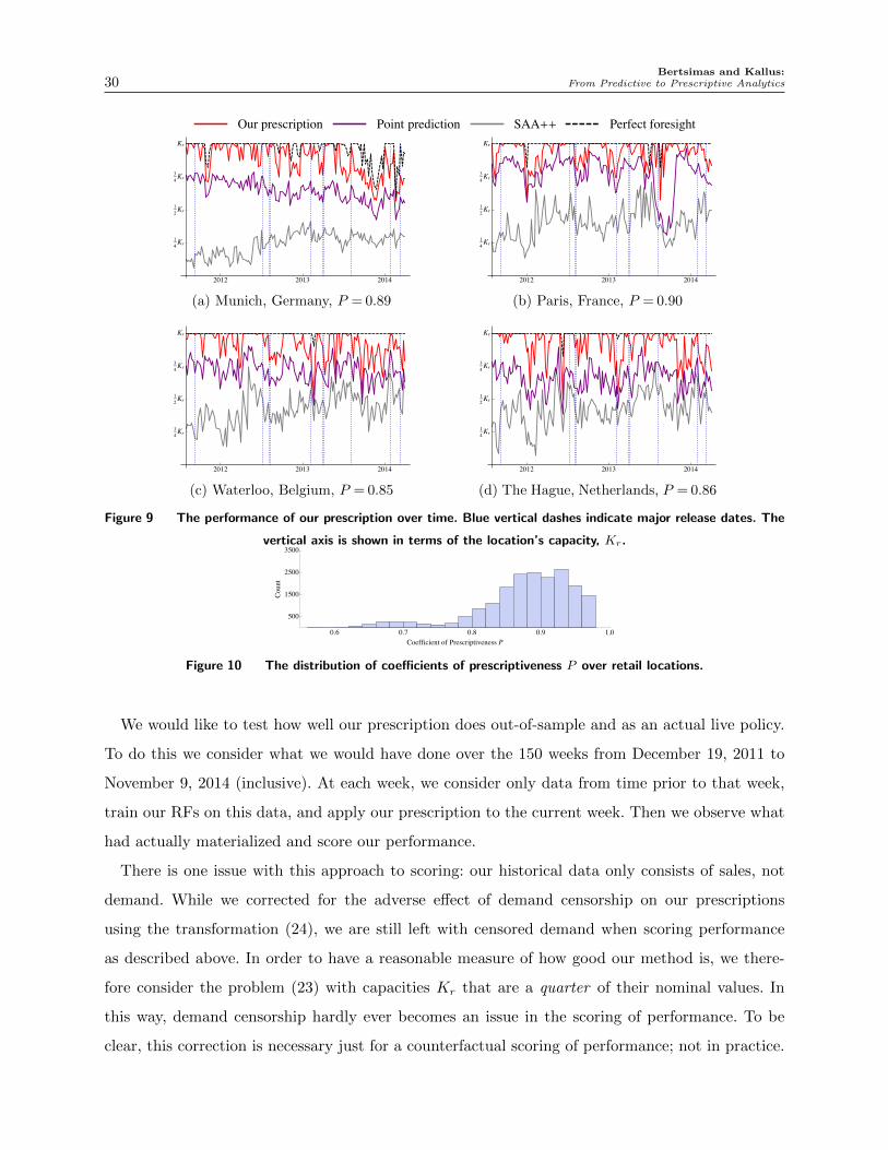
Bertsimas and Kallus:30 From Predictive to Prescriptive Analytics
��� ������������ ����� ���������� ���++ ������� ���������
���� ���� ����
����
����
����
��
(a) Munich, Germany, P = 0.89
���� ���� ����
����
����
����
��
(b) Paris, France, P = 0.90
���� ���� ����
����
����
����
��
(c) Waterloo, Belgium, P = 0.85
���� ���� ����
����
����
����
��
(d) The Hague, Netherlands, P = 0.86
Figure 9 The performance of our prescription over time. Blue vertical dashes indicate major release dates. The
vertical axis is shown in terms of the location’s capacity, Kr.
0.6 0.7 0.8 0.9 1.0
500
1500
2500
3500
Coefficient of Prescriptiveness P
Count
Figure 10 The distribution of coe�cients of prescriptiveness P over retail locations.
We would like to test how well our prescription does out-of-sample and as an actual live policy.
To do this we consider what we would have done over the 150 weeks from December 19, 2011 to
November 9, 2014 (inclusive). At each week, we consider only data from time prior to that week,
train our RFs on this data, and apply our prescription to the current week. Then we observe what
had actually materialized and score our performance.
There is one issue with this approach to scoring: our historical data only consists of sales, not
demand. While we corrected for the adverse e↵ect of demand censorship on our prescriptions
using the transformation (24), we are still left with censored demand when scoring performance
as described above. In order to have a reasonable measure of how good our method is, we there-
fore consider the problem (23) with capacities Kr that are a quarter of their nominal values. In
this way, demand censorship hardly ever becomes an issue in the scoring of performance. To be
clear, this correction is necessary just for a counterfactual scoring of performance; not in practice.
Bertsimas and Kallus:From Predictive to Prescriptive Analytics 31
The transformation (24) already corrects for prescriptions trained on censored observations of the
quantity Y that a↵ects true costs.
We compare the performance of our method with three other quantities. One is the performance
of the perfect-forecast policy, which knows future demand exactly (no distributions). Another is the
performance of a data-driven policy without access to the auxiliary data (i.e., SAA). Because the
decay of demand over the lifetime of a product is significant, to make it a fair comparison we let this
policy depend on the distributions of product demand based on how long its been on the market.
That is, it is based on T separate datasets where each consists of the demands for a product after t
weeks on the market (again, considering only past data). Due to this handicap we term it SAA++
henceforth. The last benchmark is the performance of a point-prediction-driven policy using the
RF sale prediction. Because there are a multitude of optimal solutions zj to (23) if we were to let
Yj be deterministic and fixed as our prediction mN,j(x), we have to choose a particular one for the
point-prediction-driven decision. The one we choose sets order levels to match demand and scale
to satisfy the capacity constraint: zpoint-predN,j (x) = Kr max{0, mN,j(x)}/Pd
j0=1 max{0, mN,j0(x)}.The ratio of the di↵erence between our performance and that of the prescient policy and the
di↵erence between the performance of SAA++ and that of the prescient policy is the coe�cient of
prescriptiveness P . When measured out-of-sample over the 150-week period as these policies make
live decisions, we get P = 0.88. Said another way, in terms of our objective (sales volumes), our
data X and our prescription zN(x) gets us 88% of the way from the best data-poor decision to the
impossible perfect-foresight decision. This is averaged over just under 20,000 locations.
In Figure 9, we plot the performance over time at four specific locations, the city of which is
noted. Blue vertical dashes in each plot indicate the release dates of the 10 biggest first-week sellers
in each location, which turn out to be the same. Two pairs of these coincide on the same week. The
plots show a general ordering of performance with our policy beating the point-prediction-driven
policy (but not always as seen in a few days in Figure 9b), which in turn beats SAA++ (but not
always as seen in a few days in Figure 9d). The P of our policy specific to these locations are 0.89,
0.90, 0.85, and 0.86. The corresponding P of the point-prediction-driven policy are 0.56, 0.57, 0.50,
0.40. That the point-prediction-driven policy outperforms SAA++ (even with the handicap) and
provides a significant improvement as measured by P can be attributed to the informativeness of
the data collected in Section 6.3 about demand. On most major release dates, the point-prediction-
driven policy does relatively worse, which can be attributed to the fact that demand for new
releases has the greatest amount of (residual) uncertainty, which the point-prediction-driven policy
ignores. When we leverage this data in a manner appropriate for inventory management using our
approach, we nearly double the improvement. We also see that on most major release dates, our
policy seizes the opportunity to match the perfect foresight performance, but on a few it falls short.
In Figure 10, we plot the overall distribution of P of our policy over all retail locations in Europe.
Bertsimas and Kallus:32 From Predictive to Prescriptive Analytics
7. Concluding Remarks
In this paper, we combine ideas from ML and OR/MS in developing a framework, along with
specific methods, for using data to prescribe optimal decisions in OR/MS problems that leverage
auxiliary observations. We motivate our methods based on existing predictive methodology from
ML, but, in the OR/MS tradition, focus on the making of a decision and on the e↵ect on costs,
revenues, and risk. Our approach is generally applicable, tractable, asymptotically optimal, and
leads to substantive and measurable improvements in a real-world context.
We feel that the above qualities, together with the growing availability of data and in particular
auxiliary data in OR/MS applications, a↵ord our proposed approach a potential for substantial
impact in the practice of OR/MS.
Acknowledgments
The authors would like to thank the anonymous reviewers and associate editor for their very helpful sug-
gestions that helped us improve the paper. We would like to thank Ross Anderson and David Nachum of
Google for assistance in obtaining access to Google Trends data. This paper is based upon work supported
by the National Science Foundation Graduate Research Fellowship under Grant No. 1122374.
References
Altman, Naomi S. 1992. An introduction to kernel and nearest-neighbor nonparametric regression. The
American Statistician 46(3) 175–185.
Arya, Sunil, David Mount, Nathan Netanyahu, Ruth Silverman, Angela Wu. 1998. An optimal algorithm
for approximate nearest neighbor searching in fixed dimensions. J. ACM 45(6) 891–923.
Asur, Sitaram, Bernardo Huberman. 2010. Predicting the future with social media. WI-IAT . 492–499.
Bartlett, Peter, Shahar Mendelson. 2003. Rademacher and gaussian complexities: Risk bounds and structural
results. J. Mach. Learn. Res. 3 463–482.
Belloni, Alexandre, Victor Chernozhukov. 2011. `1-penalized quantile regression in high-dimensional sparse
models. The Annals of Statistics 39(1) 82–130.
Ben-Tal, Aharon, Laurent El Ghaoui, Arkadi Nemirovski. 2009. Robust optimization. Princeton University
Press.
Bentley, Jon. 1975. Multidimensional binary search trees used for associative searching. Commun. ACM
18(9) 509–517.
Beran, Rudolf. 1981. Nonparametric regression with randomly censored survival data. Tech. rep., Technical
Report, Univ. California, Berkeley.
Berger, James O. 1985. Statistical decision theory and Bayesian analysis . Springer.
Bertsekas, Dimitri, Angelia Nedic, Asuman Ozdaglar. 2003. Convex analysis and optimization. Athena
Scientific, Belmont.

Bertsimas and Kallus:From Predictive to Prescriptive Analytics 33
Bertsekas, Dimitri P. 1995. Dynamic programming and optimal control . Athena Scientific Belmont, MA.
Bertsekas, Dimitri P. 1999. Nonlinear programming . Athena Scientific, Belmont.
Bertsimas, Dimitris, David B Brown, Constantine Caramanis. 2011. Theory and applications of robust
optimization. SIAM review 53(3) 464–501.
Bertsimas, Dimitris, Vishal Gupta, Nathan Kallus. 2013. Data-driven robust optimization Submitted to
Operations Research.
Bertsimas, Dimitris, Vishal Gupta, Nathan Kallus. 2014. Robust saa Submitted to Mathematical Program-
ming.
Bertsimas, Dimitris, Nathan Kallus. 2016. Pricing from observational data .
Besbes, Omar, Assaf Zeevi. 2009. Dynamic pricing without knowing the demand function: Risk bounds and
near-optimal algorithms. Operations Research 57(6) 1407–1420.
Billingsley, P. 1999. Convergence of Probability Measures . Wiley, New York.
Birge, John R, Francois Louveaux. 2011. Introduction to stochastic programming . Springer.
Blondel, Vincent D, Jean-Loup Guillaume, Renaud Lambiotte, Etienne Lefebvre. 2008. Fast unfolding of
communities in large networks. Journal of Statistical Mechanics: Theory and Experiment 2008(10)
P10008.
Bradley, Richard. 1986. Basic properties of strong mixing conditions. Dependence in Probability and Statis-
tics. Birkhausser, 165–192.
Bradley, Richard. 2005. Basic properties of strong mixing conditions. A survey and some open questions.
Probab. Surv. 2(107-44) 37.
Breiman, Leo. 2001. Random forests. Machine learning 45(1) 5–32.
Breiman, Leo, Jerome Friedman, Charles Stone, Richard Olshen. 1984. Classification and regression trees .
CRC press.
Calafiore, Giuseppe, Marco C Campi. 2005. Uncertain convex programs: randomized solutions and confidence
levels. Mathematical Programming 102(1) 25–46.
Calafiore, Giuseppe Carlo, Laurent El Ghaoui. 2006. On distributionally robust chance-constrained linear
programs. Journal of Optimization Theory and Applications 130(1) 1–22.
Cameron, A Colin, Pravin K Trivedi. 2005. Microeconometrics: methods and applications . Cambridge
university press.
Carrasco, Marine, Xiaohong Chen. 2002. Mixing and moment properties of various garch and stochastic
volatility models. Econometric Theory 18(1) 17–39.
Choi, Hyunyoung, Hal Varian. 2012. Predicting the present with google trends. Econ. Rec. 88(s1) 2–9.
Bertsimas and Kallus:34 From Predictive to Prescriptive Analytics
Cleveland, William S, Susan J Devlin. 1988. Locally weighted regression: an approach to regression analysis
by local fitting. Journal of the American Statistical Association 83(403) 596–610.
Da, Zhi, Joseph Engelberg, Pengjie Gao. 2011. In search of attention. J. Finance 66(5) 1461–1499.
Delage, E, Y Ye. 2010. Distributionally robust optimization under moment uncertainty with application to
data-driven problems. Operations Research 55(3) 98–112.
Devroye, Luc P, TJ Wagner. 1980. On the l 1 convergence of kernel estimators of regression functions with
applications in discrimination. Zeitschrift fur Wahrscheinlichkeitstheorie und verwandte Gebiete 51(1)
15–25.
Doukhan, Paul. 1994. Mixing: Properties and Examples. Springer.
Dudley, Richard M. 2002. Real analysis and probability , vol. 74. Cambridge University Press, Cambridge.
Fan, Jianqing. 1993. Local linear regression smoothers and their minimax e�ciencies. The Annals of Statistics
196–216.
Geer, Sara A. 2000. Empirical Processes in M-estimation, vol. 6. Cambridge university press.
Goel, Sharad, Jake Hofman, Sebastien Lahaie, David Pennock, Duncan Watts. 2010. Predicting consumer
behavior with web search. PNAS 107(41) 17486–17490.
Grotschel, M, L Lovasz, A Schrijver. 1993. Geometric algorithms and combinatorial optimization. Springer,
New York.
Gruhl, Daniel, Laurent Chavet, David Gibson, Jorg Meyer, Pradhan Pattanayak, Andrew Tomkins, J Zien.
2004. How to build a WebFountain: An architecture for very large-scale text analytics. IBM Syst. J.
43(1) 64–77.
Gruhl, Daniel, Ramanathan Guha, Ravi Kumar, Jasmine Novak, Andrew Tomkins. 2005. The predictive
power of online chatter. SIGKDD . 78–87.
Hanasusanto, Grani Adiwena, Daniel Kuhn. 2013. Robust data-driven dynamic programming. Advances in
Neural Information Processing Systems. 827–835.
Hannah, Lauren, Warren Powell, David M Blei. 2010. Nonparametric density estimation for stochastic
optimization with an observable state variable. Advances in Neural Information Processing Systems.
820–828.
Hansen, Bruce E. 2008. Uniform convergence rates for kernel estimation with dependent data. Econometric
Theory 24(03) 726–748.
Huh, Woonghee Tim, Retsef Levi, Paat Rusmevichientong, James B Orlin. 2011. Adaptive data-driven
inventory control with censored demand based on kaplan-meier estimator. Operations Research 59(4)
929–941.
Imbens, Guido W, Donald B Rubin. 2015. Causal inference in statistics, social, and biomedical sciences.
Cambridge University Press.

Bertsimas and Kallus:From Predictive to Prescriptive Analytics 35
Kakade, Sham, Karthik Sridharan, Ambuj Tewari. 2008. On the complexity of linear prediction: Risk bounds,
margin bounds, and regularization. NIPS . 793–800.
Kallus, Nathan. 2014. Predicting crowd behavior with big public data. WWW . 23, 625630.
Kao, Yi-hao, Benjamin V Roy, Xiang Yan. 2009. Directed regression. Advances in Neural Information
Processing Systems . 889–897.
Kaplan, Edward L, Paul Meier. 1958. Nonparametric estimation from incomplete observations. Journal of
the American statistical association 53(282) 457–481.
Kleywegt, Anton, Alexander Shapiro, Tito Homem-de Mello. 2002. The sample average approximation
method for stochastic discrete optimization. SIAM J. Optim. 12(2) 479–502.
Koenker, Roger. 2005. Quantile regression. 38, Cambridge university press.
Lai, Tze Leung, Herbert Robbins. 1985. Asymptotically e�cient adaptive allocation rules. Advances in
applied mathematics 6(1) 4–22.
Ledoux, Michel, Michel Talagrand. 1991. Probability in Banach Spaces: isoperimetry and processes. Springer.
Lehmann, Erich Leo, George Casella. 1998. Theory of point estimation, vol. 31. Springer.
Mcdonald, Daniel, Cosma Shalizi, Mark Schervish. 2011. Estimating beta-mixing coe�cients. AISTATS .
516–524.
Mohri, Mehryar, Afshin Rostamizadeh. 2008. Rademacher complexity bounds for non-iid processes. NIPS .
1097–1104.
Mohri, Mehryar, Afshin Rostamizadeh, Ameet Talwalkar. 2012. Foundations of machine learning . MIT
press.
Mokkadem, Abdelkader. 1988. Mixing properties of arma processes. Stochastic Process. Appl. 29(2) 309–315.
Nadaraya, Elizbar. 1964. On estimating regression. Theory Probab. Appl. 9(1) 141–142.
Nemirovski, Arkadi, Anatoli Juditsky, Guanghui Lan, Alexander Shapiro. 2009. Robust stochastic approxi-
mation approach to stochastic programming. SIAM Journal on Optimization 19(4) 1574–1609.
Parzen, Emanuel. 1962. On estimation of a probability density function and mode. The annals of mathe-
matical statistics 1065–1076.
Robbins, Herbert. 1952. Some aspects of the sequential design of experiments. Bulletin of the American
Mathematical Society 58 527–535.
Robbins, Herbert, Sutton Monro. 1951. A stochastic approximation method. The annals of mathematical
statistics 400–407.
Rosenbaum, Paul R, Donald B Rubin. 1983. The central role of the propensity score in observational studies
for causal e↵ects. Biometrika 70(1) 41–55.
Rudin, Cynthia, Gah-Yi Vahn. 2014. The big data newsvendor: Practical insights from machine learning .

Bertsimas and Kallus:36 From Predictive to Prescriptive Analytics
Shapiro, Alexander. 2003. Monte carlo sampling methods. Handbooks Oper. Res. Management Sci. 10
353–425.
Shapiro, Alexander, Arkadi Nemirovski. 2005. On complexity of stochastic programming problems. Contin-
uous optimization. Springer, 111–146.
Tibshirani, Robert. 1996. Regression shrinkage and selection via the lasso. Journal of the Royal Statistical
Society. Series B (Methodological) 267–288.
Trevor, Hastie, Tibshirani Robert, Jerome Friedman. 2001. The Elements of Statistical Learning , vol. 1.
Springer.
Vapnik, Vladimir. 1992. Principles of risk minimization for learning theory. Advances in neural information
processing systems . 831–838.
Vapnik, Vladimir. 2000. The nature of statistical learning theory . springer.
Wald, Abraham. 1949. Statistical decision functions. The Annals of Mathematical Statistics 165–205.
Walk, Harro. 2010. Strong laws of large numbers and nonparametric estimation. Recent Developments in
Applied Probability and Statistics. Springer, 183–214.
Ward, Joe. 1963. Hierarchical grouping to optimize an objective function. J. Am. Stat. Assoc. 58(301)
236–244.
Watson, Geo↵rey. 1964. Smooth regression analysis. Sankhya A 359–372.
Bertsimas and Kallus:From Predictive to Prescriptive Analytics 37
Supplement
8. Alternative Approaches using Empirical Risk Minimization
In the beginning of Section 2, we noted that the empirical distribution is insu�cient for approx-
imating the full-information problem (2). The solution was to consider local neighborhoods in
approximating conditional expected costs; these were computed separately for each x. Another
approach would be to develop an explicit decision rule and impose structure on it. In this section,
we consider an approach to constructing a predictive prescription by selecting from a family of
linear functions restricted in some norm,
F =�z(x) = Wx : W 2Rdz⇥dx , ||W ||R
, (25)
so to minimize the empirical marginal expected costs as in (4),
zN(·)2 argminz(·)2F1N
PN
i=1 c(z(xi);yi).
The linear decision rule can be generalized by transforming X to include nonlinear terms or by
embedding in a reproducing kernel Hilbert space. We consider two examples of a norm on the matrix
of linear coe�cients, W : the row-wise p, p0-norm and the Schatten p-norm, which are, respectively,
||W || = ||(�1kW1kp, . . . ,�dkWdkp)||p0 , ||W || =����(⌧1, . . . , ⌧min{dz ,dx})
����p,
where ⌧i are W ’s singular values. For example, the Schatten 1-norm is the matrix nuclear norm. In
either case, the restriction on the norm is equivalent to an appropriately-weighted regularization
term incorporated into the objectives of (4).
Problem (4) corresponds to the traditional framework of empirical risk minimization in statis-
tical learning with a general loss function. It is also closely related to M -estimation Geer (2000),
except that we are concerned with out-of-sample performance rather than inference, an infinite-
dimensional decision rule rather than a finite-dimensional parameter, and potentially non-smooth
functions. For dz = dy = 1, Z = R, and c(z;y) = (z � y)2, problem (4) corresponds to least-squares
regression. For dz = dy = 1, Z = R, and c(z;y) = (y� z)(⌧ � I [y� z < 0]), problem (4) corresponds
to quantile regression (cf. Koenker (2005)), which estimates the conditional ⌧ -quantile as a func-
tion of x. Rearranging terms, c(z;y) = (y � z)(⌧ � I [y� z < 0]) = max{(1� ⌧)(z � y), ⌧(y� z)} is
the same as the newsvendor cost function where ⌧ is the service level requirement as observed by
Rudin and Vahn (2014). Standard ERM generalization theory deals only with univariate-valued
functions. Because most OR/MS problems involve multivariate uncertainty and decisions, in this
section we generalize the approach and its associated theoretical guarantees to such multivariate
problems (dy � 1, dz � 1). In particular, we generalize Rademacher complexity to multivariate-
valued decision rules and extend the Rademacher comparison Lemma (Theorem 4.12 of Ledoux

Bertsimas and Kallus:38 From Predictive to Prescriptive Analytics
and Talagrand (1991)) to this new definition. We can then apply standard results to obtain out-
of-sample guarantees.
Before continuing, we note a few limitations of any approach based on (4). For general problems,
there is no reason to expect that optimal solutions will have a linear structure (whereas certain
distributional assumptions lead to such conclusions in least-squares and quantile regression analy-
ses). In particular, unlike the predictive prescriptions studied in Section 2, the approach based on
(4) does not enjoy the same universal guarantees of asymptotic optimality. Instead, we will only
have out-of-sample guarantees that depend on our class F of decision rules.
Another limitation is the di�culty in restricting the decisions to a constrained feasible set Z 6=Rdz . Consider, for example, the portfolio allocation problem from Section 1.1, where we must havePdx
i=1 zi = 1. One approach to applying (4) to this problem might be to set c(z;y) = 1 for z /2 Z(or, equivalently, constrain z(xi) 2Z 8i). However, not only will this not guarantee that z(x) 2Zfor x outside the dataset, but we would also run into a problem of infeasibility as we would have
N linear equality constraints on dz ⇥ dx linear coe�cients (a constraint such asPdx
i=1 zi 1 that
does not reduce the a�ne dimension will still lead to an undesirably flat linear decision rule as N
grows). Another approach may be to compose F with a projection onto Z, but this will generally
lead to a non-convex optimization problem that is intractable to solve. Therefore, the approach is
limited in its applicability to OR/MS problems.
In a few limited cases, we may be able to sensibly extend the cost function synthetically outside
the feasible region while maintaining convexity. For example, in the shipment planning example of
Section 1.1, we may allow negative order quantities z and extend the first-stage costs to depend
only on the positive part of z, i.e. p1
Pdz
i=1 max{zi, 0} (but leave the second-stage costs as they are
for convexity). Now, if after training zN(·), we transform any resulting decision by only taking the
positive part of each order quantity, we end up with a feasible decision rule whose costs are no
worse than the synthetic costs of the original rule.
In the rest of this section we consider the application of the approach (4) to problems where y
and z are multivariate and c(z;y) is general, but only treat unconstrained decisions Z = Rdz .
8.1. Tractability
We first develop su�cient conditions for the problem (4) to be optimized in polynomial time. The
proof appears in Section 11.
Theorem 12. Suppose that c(z;y) is convex in z for every fixed y and let oracles be given for
evaluation and subgradient in z. Then for any fixed x we can find an ✏-optimal solution to (4) in
time and oracle calls polynomial in n, d, log(1/✏) for F as in (25).
Bertsimas and Kallus:From Predictive to Prescriptive Analytics 39
8.2. Out-of-Sample Guarantees
Next, we characterize the out-of-sample guarantees of a predictive prescription derived from (4).
All proofs are in the E-companion. In the traditional framework of empirical risk minimization in
statistical learning such guarantees are often derived using Rademacher complexity but these only
apply to univariate problems (c.f. Bartlett and Mendelson (2003)). Because most OR/MS problems
are multivariate, we generalize this theory appropriately. We begin by generalizing the definition
of Rademacher complexity to multivariate-valued functions.
Definition 3. Given a sample SN = {s1, . . . , sN}, The empirical multivariate Rademacher com-
plexity of a class of functions F taking values in Rd is defined as
bRN(F ;SN) = Eh
2N
supg2FPn
i=1
Pd
k=1 �ikgk(si)���s1, . . . , sn
i
where �ik are independently equiprobably +1,�1. The marginal multivariate Rademacher com-
plexity is defined as the expectation over the sampling distribution of SN : RN(F) = EhbRn(F ;SN)
i.
Note that given only data SN , the quantity bRN(F ;SN) is observable. Note also that when d = 1
the above definition coincides with the common definition of Rademacher complexity.
The theorem below relates the multivariate Rademacher complexity of F to out-of-sample guar-
antees on the performance of the corresponding predictive prescription zN(x) from (4). A general-
ization of the following to mixing processes is given in the supplemental Section 10. We denote by
SxN = {x1, . . . , xN} the restriction of our sample to data on X.
Theorem 13. Suppose c(z;y) is bounded and equi-Lipschitz in z:
supz2Z, y2Y c(z;y) c, supz 6=z02Z, y2Yc(z;y)�c(z0;y)
||zk�z0k||1
L <1.
Then, for any � > 0, each of the following events occurs with probability at least 1� �,
E [c(z(X);Y )] 1N
PN
i=1 c(z(xi);yi) + cp
log(1/�0)/2N + LRN(F) 8z 2F , (26)
E [c(z(X);Y )] 1N
PN
i=1 c(z(xi);yi) + 3cp
log(2/�00)/2N + LbRN(F ;SxN) 8z 2F . (27)
In particular, these hold for z = zN(·)2F .
Equations (26) and (27) provide a bound on the out-of-sample performance of any predictive
prescription z(·) 2 F . The bound is exactly what we minimize in problem (4) because the extra
terms do not depend on z(·). That is, we minimize the empirical risk, which, with additional
confidence terms, bounds the true out-of-sample costs of the resulting predictive prescription zN(·).To prove Theorem 13, we first establish a comparison lemma that is an extension of Theorem
4.12 of Ledoux and Talagrand (1991) to our multivariate case.
Lemma 1. Suppose that c is L-Lipschitz uniformly over y with respect to 1-norm:
supz 6=z02Z, y2Y
c(z;y)� c(z0;y)
maxk=1, ..., d |zk � z0k|
L <1.

Bertsimas and Kallus:40 From Predictive to Prescriptive Analytics
Let G = {(x, y) 7! c (f(x);y) : f 2F}. Then we have that bRn(G;SN)LbRn(F ;SxN) and therefore
also that Rn(G)LRn(F). (Notice that one is a univariate complexity and one multivariate and
that the complexity of F involves only the sampling of x.)
Proof Write �i(z) = c(z;yi)/L. Then by Lipschitz assumption and by part 2 of Proposition 2.2.1
from Bertsekas et al. (2003), for each i, �i is 1-Lipchitz. We now would like to show the inequality
in
bRn(G;SN) = E
"2
nsupz2F
nX
i=1
�i0�i(z(xi))
����� SN
#
LE
"2
nsupz2F
nX
i=1
dX
k=1
�ikzk(xi)
����� SxN
#
= LbRn(F ;SxN).
By conditioning and iterating, it su�ces to show that for any T ⇢R⇥Z and 1-Lipchitz �,
E
supt,z2T
(t+�0�(z))
�E
"supt,z2T
t+
dX
k=1
�kzk
!#. (28)
The expectation on the left-hand-side is over two values (�0 = ±1) so there are two choices of (t, z),
one for each scenario. Let any (t(+1), z(+1)), (t(�1), z(�1)) 2 T be given. Let k⇤ and s⇤ = ±1 be such
that
maxk=1, ..., d
���z(+1)k � z
(�1)k
���= s⇤⇣z
(+1)k⇤ � z
(�1)k⇤
⌘.
Fix (t(±1), z(±1)) = (t(±s⇤), z(±s⇤)). Then, since these are feasible choices in the inner supremum,
choosing (t, z)(�) = (t(�k⇤ ), z(�k⇤ )), we see that the right-hand-side of (28) has
RHS (28)� 1
2E
"t(+1) + z
(+1)k⇤ +
X
k 6=k⇤�kz
(+1)k
#
+1
2E
"t(�1) � z
(�1)k⇤ +
X
k 6=k⇤�kz
(�1)k
#
=1
2
✓t(+1) + t(�1) + max
k=1, ..., d
���z(+1)k � z
(�1)k
���◆
� 1
2
�t(+1) +�
�z(+1)
��+
1
2
�t(�1) ��
�z(�1)
��
where the last inequality is due to the Lipschitz condition. Since true for any (t(±1), z(±1)) given,
taking suprema over the left-hand-side completes the proof. ⇤Next, we restate the main result of Bartlett and Mendelson (2003):
Theorem 14. Consider a class G of functions U !R that are bounded: |g(u)| g 8g 2 G, u2 U .
Consider a sample Sn = (u1, . . . , uN) of some random variable T 2 T . Fix � > 0. Then we have
that, with probability 1� �,
E [g(T )] 1
N
NX
i=1
g(ui) + gp
log(1/�)/2N + RN(G) 8g 2 G, (29)
Bertsimas and Kallus:From Predictive to Prescriptive Analytics 41
and that, again with probability 1� �,
E [g(T )] 1
N
NX
i=1
g(ui) + 3gp
log(2/�)/2N + bRN(G) 8g 2 G. (30)
Finally, we can prove Theorem 13:
Proof of Theorem 13 Apply Theorem 14 to the random variable U = (X,Y ) and function class
G = {(x, y) 7! c (f(x);y) : f 2F}. Note that by assumption we have boundedness of functions in Gby the constant c. Bound the complexity of G by that of F using Lemma 1 and the assumption of
c(z;y) being L-Lipschitz. Equations (32) and (33) hold for every g 2 G and hence for every f 2Fand g(x, y) = c (f(x);y), of which the expectation is the expected costs of the decision rule f . ⇤
Equations (26) and (27) in Theorem 13 involve the multivariate Rademacher complexity of our
class F of decision rules. In the next lemmas, we compute appropriate bounds on the complexity
of our examples of classes F . The theory, however, applies beyond linear rules.
Lemma 2. Consider F as in (25) with row-wise p, p0 norm for p 2 [2,1) and p0 2 [1,1]. Let q
be the conjugate exponent of p (1/p+ 1/q = 1) and suppose that ||x||q M for all x2X . Then
RN(F) 2MRq
p�1N
Pdz
k=11�k
.
Lemma 3. Consider F as in (25) with Schatten p-norm. Let r = max{1� 1/p, 1/2}. Then
bRN(F ;SxN) 2Rdr
z
q1N
q1N
PN
i=1 kxik, RN(F) 2Rdrz
q1N
qE ||X||22.
The above results indicate that the confidence terms in equations (26) and (27) shrink to 0 as
N !1 even if we slowly relax norm restrictions. Hence, we can approach the optimal out-of-sample
performance over the class F without restrictions on norms.
Proof of Lemma 2 Consider Fk = {zk(·) : z 2F} = {zk(x) = wT x : ||w||p R�k
}, the projection of
F onto the kth coordinate. Then F ⇢F1 ⇥ · · ·⇥Fdz and RN(F)Pdz
k=1 RN(Fk). The latter right-
hand-side complexities are the common univariate Rademacher complexities. Applying Theorem 1
of Kakade et al. (2008) to each component we get RN(Fk) 2Mq
p�1N
R�k
. ⇤Proof of Lemma 3 Let q be p’s conjugate exponent (1/p + 1/q = 1). In terms of vector norms
on v 2 Rd, if q � 2 then ||v||p ||v||2 and if q 2 then ||b||p d1/2�1/p ||v||2. Let F be the matrix
Fji = xij. Note that F� 2Rdx⇥dz . By Jensen’s inequality and since Schatten norms are vector norms
on singular values,
bR2N(F ;Sx
N) 4
N 2E
"sup
||W ||pR
Trace (WF�)2
����SxN
#
=4R2
N 2Eh||F�||2q
��SxN
i
4R2
N 2max
nmin{dz, dx}1�2/p
,1o
Eh||F�||22
��SxN
i
4R2
N 2max
�d1�2/p
z ,1
Eh||F�||22
��SxN
i.

Bertsimas and Kallus:42 From Predictive to Prescriptive Analytics
The first result follows because
1
NEh||F�||22
��SxN
i=
1
n
dzX
k=1
dxX
j=1
NX
i,i0=1
xijx
i0j E [�ik�i0k]
=dz
N
NX
i=1
dxX
j=1
(xij)
2 = dzbEN ||x||22
The second result follows by applying Jensen’s inequality again to pass the expectation over Sn
into the square. ⇤
9. Extensions of Asymptotic Optimality to Mixing Processes andProofs
In this supplemental section, we generalize the asymptotic results to mixing process and provide
the omitted proofs from Sections 4.3 and 4.4.
9.1. Mixing Processes
We begin by defining stationary and mixing processes.
Definition 4. A sequence of random variables V1, V2, . . . with joint measure µ is called sta-
tionary if joint distributions of finitely many consecutive variables are invariant to shifting. That
is,
µVt,...,Vt+k= µVs,...,Vs+k
8s, t2N, k � 0,
where µVt,...,Vt+kis the induced measure on a sequence of length k.
In particular, if a sequence is stationary then the variables have identical marginal distributions,
but they may not be independent and the sequence may not be exchangeable. Instead of inde-
pendence, mixing is the property that if standing at particular point in the sequence we look far
enough ahead, the head and the tail look nearly independent, where “nearly” is defined by di↵erent
metrics for di↵erent definitions of mixing.
Definition 5. Given a stationary sequence {Vt}t2N, denote by At = � (V1, . . . , Vt) the sigma-
algebra generated by the first t variables and by At = � (Vt, Vt+1, . . . ) the sigma-algebra generated
by the subsequence starting at t. Define the mixing coe�cients at lag k
↵(k) = supt2N,A2At,B2At+k
|µ(A\B)�µ(A)µ(B)|
�(k) = supt2N
������µ{Vs}st
⌦µ{Vs}s�t+k�µ{Vs}st_s�t+k
������TV
⇢(k) = supt2N,Q2L2(At),R2L2(At+k)
|Corr(Q,R)|
where ||·||TV is the total variance and L2(A) is the set of A-measurable square-integrable real-valued
random variables.
{Vt} is said to be ↵-mixing if ↵(k)k!1�! 0 , �-mixing if �(k)
k!1�! 0, and ⇢-mixing if ⇢(k)k!1�! 0.

Bertsimas and Kallus:From Predictive to Prescriptive Analytics 43
Notice that an iid sequence has ↵(k) = �(k) = ⇢(k) = 0. Bradley (1986) establishes that 2↵(k)�(k) and 4↵(k) ⇢(k) so that either �- or ⇢-mixing implies ↵-mixing.
Many processes satisfy mixing conditions under mild assumptions: auto-egressive moving-
average (ARMA) processes (cf. Mokkadem (1988)), generalized autoregressive conditional heteros-
kedasticity (GARCH) processes (cf. Carrasco and Chen (2002)), and certain Markov chains. For a
thorough discussion and more examples see Doukhan (1994) and Bradley (2005). Mixing rates are
often given explicitly by model parameters but they can also be estimated from data (cf. Mcdonald
et al. (2011)). Sampling from such processes models many real-life sampling situations where obser-
vations are taken from an evolving system such as, for example, the stock market, inter-dependent
product demands, or aggregates of doubly stochastic arrival processes as in the posts on social
media.
9.2. Asymptotic Optimality
Let us now restate the results of Section 4.3 in more general terms, encompassing both iid and
mixing conditions on SN .
Theorem 15 (kNN). Suppose Assumptions 3, 4, and 5 hold and that SN is generated by iid
sampling. Let wN,i(x) be as in (12) with k = min�dCN �e,N � 1
for some C > 0, 0 < � < 1. Let
zN(x) be as in (3). Then zN(x) is asymptotically optimal and consistent.
Theorem 16 (Kernel Methods). Suppose Assumptions 3, 4, and 5 hold and that
E [|c(z;Y )|max{log |c(z;Y )| ,0}] <1 for each z. Let wN,i(x) be as in (13) with K being any of the
kernels in Section 2.2 and h = CN�� for C, � > 0. Let zN(x) be as in (3). If SN comes from
1. an iid process and � < 1/dx, or
2. a ⇢-mixing process with ⇢(k) = O(k��) (� > 0) and � < 2�/(dx + 2dx�), or
3. an ↵-mixing process with ↵(k) = O(k��) (� > 1) and � < 2(�� 1)/(3dx + 2dx�),
then zN(x) is asymptotically optimal and consistent.
Theorem 17 (Recursive Kernel Methods). Suppose Assumptions 3, 4, and 5 hold and that
SN comes from a ⇢-mixing process withP1
k=1 ⇢(k) <1 (or iid). Let wN,i(x) be as in (14) with K
being the naıve kernel and with hi = Ci�� for some C > 0, 0 < � < 1/(2dx). Let zN(x) be as in (3).
Then zN(x) is asymptotically optimal and consistent.
Theorem 18 (Local Linear Methods). Suppose Assumptions 3, 4, and 5 hold, that µX is
absolutely continuous and has density bounded away from 0 and 1 on the support of X and twice
continuously di↵erentiable, and that costs are bounded over y for each z (i.e., |c(z;y)| g(z)) and
twice continuously di↵erentiable. Let wN,i(x) be as in (15) with K being any of the kernels in
Section 2.2 and with hN = CN�� for some C, � > 0. Let zN(x) be as in (3). If SN comes from
Bertsimas and Kallus:44 From Predictive to Prescriptive Analytics
1. an iid process and � < 1/dx, or
2. an ↵-mixing process with ↵(k) = O(k��), � > dx + 3, and � < (�� dx � 3)/(dx(�� dx + 3)),
then zN(x) is asymptotically optimal and consistent.
Theorem 19 (Nonnegative Local Linear Methods). Suppose Assumptions 3, 4, and 5
hold, that µX is absolutely continuous and has density bounded away from 0 and 1 on the sup-
port of X and twice continuously di↵erentiable, and that costs are bounded over y for each z (i.e.,
|c(z;y)| g(z)) and twice continuously di↵erentiable. Let wN,i(x) be as in (16) with K being any
of the kernels in Section 2.2 and with hN = CN�� for some C, � > 0. Let zN(x) be as in (3). If SN
comes from
1. an iid process and � < 1/dx, or
2. an ↵-mixing process with ↵(k) = O(k��), � > dx + 3, and � < (�� dx � 3)/(dx(�� dx + 3)),
then zN(x) is asymptotically optimal and consistent.
Theorem 20 (Decisions A↵ect Uncertainty). Suppose Assumptions 1, 2, 3, 4, and 5 (case
1) hold, that µ(X,Z1) is absolutely continuous and has density bounded away from 0 and 1 on the
support of X,Z1 and twice continuously di↵erentiable, and that costs are bounded over y for each z
(i.e., |c(z;y)| g(z)) and twice continuously di↵erentiable. Let wN,i(x) be as in (13), (15), or (16)
applied to SN with K being any of the kernels in Section 2.2 and with hN = CN�� for some C > 0,
� > 0. Let zN(x) be as in (21). If SN comes from
1. an iid process and � < 1/(dx + dz1), or
2. an ↵-mixing process with ↵(k) = O(k��), � > dx + dz1+ 3, and � < (�� dx � dz1
� 3)/(dx(��dx � dz1
+ 3)),
Then zN(x) is asymptotically optimal and consistent.
9.3. Proofs of Asymptotic Results for Local Predictive Prescriptions
First, we establish some preliminary results. In what follows, let
C(z|x) = E⇥c(z;Y )
��X = x⇤,
bCN(z|x) =NX
i=1
wN,i(x)c(z;yi),
µY |x(A) = E⇥I [Y 2A]
��X = x⇤,
µY |x,N(A) =NX
i=1
wN,i(x)I⇥yi 2A
⇤.
Lemma 4. If {(xi, yi)}i2N is stationary and f : RmY ! R is measurable then {(xi, f(yi))}i2N is
also stationary and has mixing coe�cients no larger than those of {(xi, yi)}i2N.

Bertsimas and Kallus:From Predictive to Prescriptive Analytics 45
Proof This is simply because a transform can only make the generated sigma-algebra coarser.
For a single time point, if f is measurable and B 2 B(R) then by definition f�1(B) 2 B(R) and,
therefore, {Y �1(f�1(B)) : B 2 B(R)} ⇢ {Y �1(B) : B 2 B(RmY )}. Here the transform is applied
independently across time so the result holds (f ⇥ · · ·⇥ f remains measurable). ⇤
Lemma 5. Suppose Assumptions 3 and 4 hold. Fix x 2X and a sample path of data such that,
for every z 2 Z, bCN(z|x) ! C(z|x). Then bCN(z|x) ! C(z|x) uniformly in z over any compact
subset of Z.
Proof Let any convergent sequence zN ! z and ✏ > 0 be given. By equicontinuity and
zN ! z, 9N1 such that |c(zN ;y)� c(z;y)| ✏/2 8N � N1. Then��� bCN(zN |x)� bCN(z|x)
��� EµY |x,N
|c(zN ;y)� c(z;y)| ✏/2 8N � N1. By assumption bCN(z|x) ! C(z|x) and hence 9N2 such
that��� bCN(z|x)�C(z|x)
��� ✏/2. Therefore, for N �max{N1,N2},��� bCN(zN |x)�C(z|x)
������ bCN(zN |x)� bCN(z|x)
���+��� bCN(z|x)�C(z|x)
��� ✏.
Hence bCN(zN |x)!C(z|x) for any convergent sequence zN ! z.
Now fix E ⇢ Z compact and suppose for contradiction that supz2E
��� bCN(z|x)�C(z|x)��� 6! 0.
Then 9✏ > 0 and zN 2 E such that��� bCN(zN |x)�C(zN |x)
��� � ✏ infinitely often. Restricting first to
a subsequence where this always happens and then using the compactness of E, there exists a
convergent subsequence zNk! z 2E such that
��� bCNk(zNk
|x)�C(zNk|x)���� ✏ for every k. Then,
0 < ✏��� bCNk
(zNk|x)�C(zNk
|x)������ bCNk
(zNk|x)�C(z|x)
���+��C(z|x)�C(zNk
|x)�� .
Since zNk! z, we have shown before that 9k1 such that
��� bCNk(zNk
|x)�C(z|x)��� ✏/2 8k � k1.
By equicontinuity and zNk! z, 9k2 such that
��c(zNk;y)� c(z;y)
�� ✏/4 8k � k2. Hence, also��C(z|x)�C(zNk
|x)�� E
⇥��c(zNk;y)� c(z;y)
�� ��X = x⇤ ✏/4 8k � k2. Considering k = max{k1, k2}
we get the contradiction that 0 < ✏ ✏/2. ⇤
Lemma 6. Suppose Assumptions 3, 4, and 5 hold. Fix x2X and a sample path of data such that
µY |x,N ! µY |x weakly and, for every z 2Z, bCN(z|x)!C(z|x). Then limN!1
⇣minz2Z bCN(z|x)
⌘=
v⇤(x) and every sequence zN 2 argminz2Z bCN(z|x) satisfies limN!1 C (zN |x) = v⇤(x) and
limN!1 infz2Z⇤(x) ||z � zN || = 0.
Proof First, we show bCN(z|x) and C(z|x) are continuous and eventually coercive. Let ✏ > 0
be given. By equicontinuity, 9� > 0 such that |c(z;y)� c(z0;y)| ✏ 8y 2 Y whenever ||z � z0|| �.
Hence, whenever ||z � z0|| �, we have��� bCN(z|x)� bCN(z0|x)
��� EµY |x,N|c(z;y)� c(z0;y)| ✏ and
|C(z|x)�C(z0|x)|E⇥|c(z;y)� c(z0;y)|
��X = x⇤ ✏. This gives continuity. Coerciveness is trivial if
Z is bounded. Suppose it is not. Without loss of generality Dx is compact, otherwise we can take any
compact subset of it that has positive probability on it. Then by assumption of weak convergence

Bertsimas and Kallus:46 From Predictive to Prescriptive Analytics
9N0 such that µY |x,N(Dx) � µY |x(Dx)/2 > 0 for all N �N0. Now let zk 2 Z be any sequence such
that ||zk|| !1. Let M > 0 be given. Let �0 = lim infk!1 infy/2Dx c(zk;y) and � = max{�0,0}. By
assumption �0 >�1. Hence 9k0 such that infy/2Dx c(zk;y)� �0 8k � k0. By Dx-uniform coerciveness
and ||zk|| ! 1, 9k1 � k0 such that c(zk;y) � (2M � 2�)/µY |x(Dx) 8k � k1 and y 2 Dx. Hence,
8k � k1 and N �N0,
C(zk|x)� µY |x(Dx)⇥ (2M � 2�)/µY |x(Dx) + (1�µY |x(Dx))�0 � 2M � 2�+��M,
bCN(zk|x)� µY |x,N(Dx)⇥ (2M � 2�)/µY |x,N(Dx) + (1� µY |x,N(Dx))�0 �M ��+�= M,
since ↵�0 � � if ↵� 0. This gives coerciveness eventually. By the usual extreme value theorem (c.f.
Bertsekas (1999), pg. 669), bZN(x) = argminz2Z bCN(z|x) and Z⇤(x) = argminz2Z C(z|x) exist, are
nonempty, and are compact.
Now we show there exists Z⇤1(x) compact such that Z⇤(x) ⇢ Z⇤
1(x) and bZN(x) ⇢ Z⇤1(x) even-
tually. If Z is bounded this is trivial. So suppose otherwise (and again, without loss of general-
ity Dx is compact). Fix any z⇤ 2 Z⇤(x). Then by Lemma 5 we have bCN(z⇤|x) ! C(z⇤|x). Since
minz2Z bCN(z|x) bCN(z⇤|x), we have limsupN!1 minz2Z bCN(z|x)C(z⇤|x) = minz2Z C(z|x) = v⇤.
Now suppose for contradiction no such Z⇤1(x) exists. Then there must be a subsequence zNk
2 bZNk
such that����zNk
����!1. By Dx-uniform coerciveness and����zNk
����!1, 9k1 � k0 such that c(zNk;y)�
2 (v⇤ + 1��)/µY |x(Dx) 8k � k1 and y 2Dx. Hence, 8k � k1 and N �N0,
bCN(zNk|x)� µY |x,N(Dx)⇥ 2 (v⇤ + 1��)/µY |x(Dx) + (1� µY |x,N(Dx))� v⇤ + 1.
This yields a contradiction v⇤ + 1 v⇤. So Z⇤1(x) exists.
Applying Lemma 5,
⌧N = supz2Z⇤1(x)
��� bCN(z|x)�C(z|x)���! 0.
The first result follows from
�N =���min
z2ZbCN(z|x)�min
z2ZC(z|x)
��� supz2Z⇤1(x)
��� bCN(z|x)�C(z|x)���= ⌧N ! 0.
Now consider any sequence zN 2 bZN(x). The second result follows from���C (zN |x)�min
z2ZC(z|x)
������ bCN(zN(x)|x)�C (zN |x)
���+���min
z2ZbCN(z|x)�min
z2ZC(z|x)
��� ⌧N + �N ! 0.
Suppose the third result is false. Then since Z⇤1(x) is compact, there is a convergent sub-
sequence zNk! z0 such that infz2Z⇤(x)
����zNk� z���� � ⌘ > 0 for all k. Since infz2Z⇤(x) ||z0 � z|| �
infz2Z⇤(x)
����zNk� z���� �
����zNk� z0���� ! ⌘ > 0, we have z0 /2 Z⇤(x) and hence ✏ = C(z0|x) �
minz2Z C(z|x) > 0. By equicontinuity and zNk! z0, 9k2 such that
��c(zNk;y)� c(z0;y)
�� ✏/2 8y 2Y 8k � k2. Then,
��C(zNk|x)�C(z0|x)
�� E⇥��c(zNk
;y)� c(z0;y)�� ��X = x
⇤ ✏/2 8k � k2. Therefore,
8k � k2,
⌧Nk+ �Nk
�C(zNk|x)�min
z2ZC(z|x)�C(z0|x)�min
z2ZC(z|x)� ✏/2 = ✏/2,

Bertsimas and Kallus:From Predictive to Prescriptive Analytics 47
which, taking limits, is a contradiction, yielding the third result. ⇤
Lemma 7. Suppose c(z;y) is equicontinuous in z. Suppose moreover that for each fixed z 2Z ⇢Rd we have that bCN(z|x)!C(z|x) a.s. for µX-a.e.x and that for each fixed measurable D ⇢Y we
have that µY |x,N(D) ! µY |x(D) a.s. for µX-a.e.x. Then, a.s. for µX-a.e.x, bCN(z|x) ! C(z|x) for
all z 2Z and µY |x,N ! µY |x weakly.
Proof Since Euclidean space is separable, µY |x,N ! µY |x weakly a.s. for µX-a.e.x (c.f. Theo-
rem 11.4.1 of Dudley (2002)). Consider the set Z 0 = Z \ Qd [ {the isolated points of Z}. Then
Z 0 is countable and dense in Z. Since Z 0 is countable, by continuity of measure, a.s. for µX-
a.e.x, bCN(z0|x) ! C(z0|x) for all z0 2 Z 0. Restrict to a sample path and x where this event
occurs. Consider any z 2 Z and ✏ > 0. By equicontinuity 9� > 0 such that |c(z;y)� c(z0;y)| ✏/2 whenever ||z � z0|| �. By density there exists such z0 2 Z 0. Then,
��� bCN(z|x)� bCN(z0|x)���
EµY |x,N[|c(z;y)� c(z0;y)|] ✏/2 and |C(z|x)�C(z0|x)|E
⇥|c(z;y)� c(z0;y)|
��X = x⇤ ✏/2. There-
fore, 0��� bCN(z|x)�C(z|x)
������ bCN(z0|x)�C(z0|x)
���+ ✏! ✏. Since true for each ✏, the result follows
for all z 2Z. The choice of particular sample path and x constitute a measure-1 event by assump-
tion. ⇤Now, we prove the general form of the asymptotic results from Section 9.2.
Proof of Theorem 15 Fix z 2 Z. Set Y 0 = c(z;y). By Assumption 3, E[|Y 0|] < 1. Let us apply
Theorem 5 of Walk (2010) to Y 0. By iid sampling and choice of k, we have that bCN(z|x)!E[Y 0|X =
x] for µX-a.e.x, a.s.
Now fix D measurable. Set Y 0 = I [y 2D]. Then E[Y 0] exists by measurability and Y 0 is bounded
in [0,1]. Therefore applying Theorem 5 of Walk (2010) in the same manner again, µY |x,N(D)
converges to µY |x(D) for µX-a.e.x a.s.
Applying Lemma 7 we obtain that assumptions for Lemma 6 hold for µX-a.e.x, a.s., which in
turn yields the result desired. ⇤Proof of Theorem 16 Fix z 2 Z. Set Y 0 = c(z;y). By Assumption 3, E[|Y 0|] < 1. Let us apply
Theorem 3 of Walk (2010) to Y 0. By assumption in theorem statement, we also have that
E{|Y 0|max{log |Y 0| ,0}} <1. Moreover each of the kernels in Section 2.2 can be rewritten K(x) =
H(||x||) such that H(0) > 0 and limt!1 tdX H(t)! 0.
Consider the case of iid sampling. Then our data on (X,Y 0) is ⇢-mixing with ⇢(k) = 0. Using
these conditions and our choices of kernel and hN , Theorem 3 of Walk (2010) gives that bCN(z|x)!E[Y 0|X = x] for µX-a.e.x, a.s.
Consider the case of ⇢-mixing or ↵-mixing. By Lemma 4, equal or lower mixing coe�cients hold
for X,Y 0 as hold for X,Y . Using these conditions and our choices of kernel and hN , Theorem 3 of
Walk (2010) gives that bCN(z|x)!E[Y 0|X = x] for µX-a.e.x, a.s.

Bertsimas and Kallus:48 From Predictive to Prescriptive Analytics
Now fix D measurable. Set Y 0 = I [y 2D]. Then E[Y 0] exists by measurability and
E{|Y 0|max{log |Y 0| ,0}} 1 <1. Therefore applying Theorem 3 of Walk (2010) in the same man-
ner again, µY |x,N(D) converges to µY |x(D) for µX-a.e.x a.s.
Applying Lemma 7 we obtain that assumptions for Lemma 6 hold for µX-a.e.x, a.s., which in
turn yields the result desired. ⇤Proof of Theorem 17 Fix z 2 Z. Set Y 0 = c(z;y). By Assumption 3, E[|Y 0|] < 1. Let us apply
Theorem 4 of Walk (2010) to Y 0. Note that the naıve kernel satisfies the necessary conditions.
Since our data on (X,Y ) is ⇢-mixing by assumption, we have that by Lemma 4, equal or lower
mixing coe�cients hold for X,Y 0 as hold for X,Y . Using these conditions and our choice of the
naıve kernel and hN , Theorem 4 of Walk (2010) gives that bCN(z|x) ! E[Y 0|X = x] for µX-a.e.x,
a.s.
Now fix D measurable. Set Y 0 = I [y 2D]. Then E[Y 0] exists by measurability. Therefore applying
Theorem 4 of Walk (2010) in the same manner again, µY |x,N(D) converges to µY |x(D) for µX-a.e.x
a.s.
Applying Lemma 7 we obtain that assumptions for Lemma 6 hold for µX-a.e.x, a.s., which in
turn yields the result desired. ⇤Proof of Theorem 18 Fix z 2Z and x2X . Set Y 0 = c(z;Y ). By Assumption 3, E[|Y 0|] <1. Let
us apply Theorem 11 of Hansen (2008) to Y 0 and use the notation thereof. Fix the neighborhood
of consideration to the point x (i.e., set cN = 0) since uniformity in x is not of interest. All of the
kernels in Section 2.2 are bounded above and square integrable and therefore satisfy Assumption 1
of Hansen (2008). Let f be the density of X. By assumption 0 < � f(x)B0 <1 for all x2X .
Moreover, our choice of hN satisfies hN ! 0.
Consider first the iid case. Then we have ↵(k) = 0 = O(k��) for � = 1 (� in Hansen (2008)).
Combined with boundedness conditions of Y 0 and f (|Y 0| g(z) < 1 and � < f < B0), we satisfy
Assumption 2 of Hansen (2008). Setting � = 1, s = 1 in (17) of Hansen (2008) we get ✓ = 1.
Therefore, since h = O(N�1/dx) we have
(log logN)4(logN)2
N ✓hdxN
! 0.
Having satisfied all the conditions of Theorem 11 of Hansen (2008), we have that bCN(z|x) !E[Y 0|X = x] a.s.
Now consider the ↵-mixing case. If the mixing conditions hold for X,Y then by Lemma 4, equal
or lower mixing coe�cients hold for X,Y 0. By letting s = 1 we have � > dx + 3 > 2. Combined
with boundedness conditions of Y 0 and f (|Y 0| g(z) <1 and � < f < B0), we satisfy Assumption
2 of Hansen (2008). Setting q = 1, s = 1 in (16) and (17) of Hansen (2008) we get ✓ = ��dx�3��dx+3
.
Therefore, since hN = O(N�✓/dx) we have
(log logN)4(logN)2
N ✓hdxN
! 0.

Bertsimas and Kallus:From Predictive to Prescriptive Analytics 49
Having satisfied all the conditions of Theorem 11 of Hansen (2008), we have again that bCN(z|x)!E[Y 0|X = x] a.s.
Since x2X was arbitrary we have convergence for µX-a.e.x a.s.
Now fix D measurable. Consider a response variable Y 0 = I [y 2D]. Then E[Y 0] exists by measur-
ability and Y 0 is bounded in [0,1]. In addition, by Lemma 4, equal or lower mixing coe�cients hold
for X,Y 0 as hold for X,Y . Therefore applying Theorem 11 of Hansen (2008) in the same manner
again, µY |x,N(D) converges to µY |x(D) for µX-a.e.x a.s.
Applying Lemma 7 we obtain that assumptions for Lemma 6 hold for µX-a.e.x, a.s., which in
turn yields the result desired. ⇤Proof of Theorem 19 Consider the unnormalized local linear weights, which we rewrite as:
wN,i(x) = ki(x)
1�
nX
j=1
kj(x)(xj �x)T⌅(x)�1(xi �x)
!
= K
✓xi �x
hN
◆✓1�hN �(x)T (x)�1
✓xi �x
hN
◆◆,
where �(x) =1
Nhd+1N
nX
j=1
K
✓xj �x
hN
◆✓xj �x
hN
◆,
(x) =1
NhdN
nX
j=1
K
✓xj �x
hN
◆✓xj �x
hN
◆✓xj �x
hN
◆T
.
We will show that wN,i(x) � 0 eventually as N grows for µX-a.e.x, a.s. Then we will have that
weights (16) are equal to weights (15) eventually and Theorem 19 applies. Let ⌃=R
K(u)uuT du,
a⇤n =
⇣logN
NhDN
⌘1/2
+h2N , and fX denote the density of X. Using the properties of the kernel (symmetric
and zero outside the unit ball) and the di↵erentiability of fX (series expandable), to show that
Eh�(x)
i=
1
hd+1N
ZK
✓x0 �x
hN
◆✓x0 �x
hN
◆fX(u)dx0
=1
hN
ZK (u)ufX(x+ hNu)du
=1
hN
ZK (u)u(fX(x) + hNrfX(x)T u+ O(h2
N ||u||2))du
=⌃rfX(x) + O(h2N),
Eh (x)
i=
1
hdN
ZK
✓x0 �x
hN
◆✓x0 �x
hN
◆✓x0 �x
hN
◆T
fX(u)dx0
=
ZK (u)uuT fX(x+ hNu)du
=
ZK (u)uuT (fX(x) + hNrfX(x)T u+ O(h2
N ||u||2))du
= fX(x)⌃+ O(h2N).
By two invocations of Theorem 2 of Hansen (2008), �(x) = ⌃rfX(x) + O(a⇤n) and (x) = ⌃r+
O(a⇤n) uniformly in x a.s. Note that K
⇣xi�xhN
⌘= 0 if
������xi�x
hN
������ > 1 so to show wN,i(x) � 0 we can

Bertsimas and Kallus:50 From Predictive to Prescriptive Analytics
restrict to������xi�x
hN
������ 1. Therefore, we have that wN,i(x) = ki(x)(1�O(hN)) where O(hN) is uni-
formly in x a.s. so that wN,i(x)� 0 for all i eventually for µX-a.e.x, a.s. ⇤Proof of Theorem 20 Fix any x. Let us redefine
C(z|x) = E⇥c(z;Y (z))
��X = x⇤, bCN(z|x) =
NX
i=1
wN,i(x, z1)c(z;yi).
Next, fix any z. Let Y 0 = c(z;Y ) and note that, by Lemma 4, the same mixing coe�cients hold
for ((X,Z1), Y0) as do for (X,Y,Z). In the case of weights given by (13), applying Theorem 9
of Hansen (2008) to ((X,Z1), Y0) yields the following uniform convergence over the inputs to the
weights (x, z1): we have that, for some cN !1, almost surely
sup||x0||+||z01||cN
�����NX
i=1
wN,i(x0, z0
1)c(z;yi)�E⇥c(z;Y )
��X = x0,Z1 = z01
⇤�����! 0. (31)
For the case of weights given by (15), applying Theorem 11 of Hansen (2008) yields the same result
(31). Finally, in the case of weights given by (16), we repeat the argument in Theorem 19 verbatim
but replacing x by (x, z1) everywhere to arrive at the conclusion that the weights are eventually
nonnegative, eventually reduce to the case of weights given by (15), and yield the same result (31).
A critical observation is that (31) holds for z01 6= z1. Now, let us restrict to the almost sure event
that (31) holds simultaneously for all z 2Z \Qdz , of which there are countably many.
Let ✏ > 0 be given. By equicontinuity, for each z 2 Z \ Qdz there is �z > 0 such that
|c(z;y)� c(z0;y)| ✏/4 for all y, ||z � z0|| �z. By density of rationals, these balls cover Z. Since Zis compact, there is a finite collection z1, . . . , zk 2Z \Qdz such that for all z 2Z there is a j such
that ||z � zj|| �zj . Let N1 be large enough so that for all N � N1, ||x|| + supz2Z ||z1|| cN and
the left-hand-side of (31) is no more than ✏/2 for each of the finitely-many z1, . . . , zk.
Let N �N1. Let any z be given. Let j be such that ||z � zj|| �zj . Note that
NX
i=1
wN,i(x, z1)c(zj;yi) = bCN(z|x) +
NX
i=1
wN,i(x, z1)(c(zj;yi)� c(z;yi)).
Moreover, by Assumptions 1 and 2, we have
E⇥c(zj;Y )
��X = x,Z1 = z1
⇤= E
⇥c(z;Y )
��X = x,Z1 = z1
⇤+ E
⇥c(zj;Y )� c(z;Y )
��X = x,Z1 = z1
⇤
= E⇥c(z;Y (z1))
��X = x⇤+ E
⇥c(zj;Y )� c(z;Y )
��X = x,Z1 = z1
⇤
= C(z|x) + E⇥c(zj;Y )� c(z;Y )
��X = x,Z1 = z1
⇤.
Therefore, since ||x|| + ||z1|| cN ,
��� bCN(z|x)�C(z|x)���=�����
NX
i=1
wN,i(x, z1)c(z;yi)�E⇥c(z;Y )
��X = x,Z1 = z1
⇤�����
NX
i=1
wN,i(x, z1)��c(z;yi)� c(zj;yi)
��+ E⇥��c(z;yi)� c(zj;yi)
�� ��X = x,Z1 = z1
⇤

Bertsimas and Kallus:From Predictive to Prescriptive Analytics 51
+
�����NX
i=1
wN,i(x, z1)c(zj;yi)�E
⇥c(zj;Y )
��X = x,Z1 = z1
⇤�����
✏/4+ ✏/4+ ✏/2 = ✏.
Since z and ✏ were arbitrary and N1 did not depend on z, we have
⌧N = supz2Z
��� bCN(z|x)�C(z|x)���! 0.
Therefore,
�N =��� infz2Z
bCN(z|x)� infz2Z
C(z|x)��� sup
z2Z
��� bCN(z|x)�C(z|x)���= ⌧N ! 0.
Next, let zN , ✏N be such that ✏N ! 0 and bCN(zN |x)� infz2Z bCN(z|x) ✏N . Then,
0C(zN |x)� infz2Z
C(z|x)��� bCN(zN |x)�C(zN |x)
���+��� bCN(zN |x)� inf
z2ZbCN(zN |x)
���
+��� infz2Z
bCN(zN |x)� infz2Z
C(z|x)��� ⌧N + ✏N + �N ! 0,
which completes the proof. ⇤Proof of Theorem 11 By assumption of Y and V sharing no atoms, �
a.s.= � = I [Y V ] is observ-
able so let us replace �i by �i in (24). Let
F (y|x) = E⇥I [Y > y]
��X = x⇤
FN(y|x) =NX
i=1
I⇥ui > y
⇤wKaplan-Meier
N,i (x),
H1(y|x) = EhIhU > y, � = 1
i ��X = xi
H1,N(y|x) =NX
i=1
Ihui > y, �i = 1
iwN,i(x),
H2(y|x) = E⇥I [U > y]
��X = x⇤
H2,N(y|x) =NX
i=1
I⇥ui > y
⇤wN,i(x).
By assumption on conditional supports of Y and V , sup{y : F (y : x) > 0} sup{y : H2(y : x) > 0}.By the same arguments as in Theorem 5, 6, 7, or 8, we have that, for all y, H1,N(y|x)!H1(y|x),
H2,N(y|x)!H2(y|x) a.s. for µX-a.e.x. By assumption of conditional independence and by the main
result of Beran (1981), we have that, for all y, FN(y|x) ! F (y|x) a.s. for µX-a.e.x. Since Y is a
separable space we can bring the “for all y” inside the statement, i.e., we have weak convergence
(c.f. Theorem 11.4.1 of Dudley (2002)): µY |x,N ! µY |x a.s. for µX-a.e.x where µY |x,N is based on
weights wKaplan-MeierN,i (x). Since costs are bounded, the portmanteau lemma (see Theorem 2.1 of
Billingsley (1999)) gives that for each z 2 Z, bCN(z|x) ! E[c(z;Y )|X = x] where bCN(z|x) is based
on weights wKaplan-MeierN,i (x). Applying Lemma 7 we obtain that assumptions for Lemma 6 hold for
µX-a.e.x, a.s., which in turn yields the result desired. ⇤

Bertsimas and Kallus:52 From Predictive to Prescriptive Analytics
10. Extensions of Out-of-Sample Guarantees to Mixing Processes andProofs
We can also extend the results of Section 8.2 to mixing processes. Combining and restating the
main results of Bartlett and Mendelson (2003) (for iid) and Mohri and Rostamizadeh (2008) (for
mixing), we can restate Theorem 14 as follows
Theorem 21. Consider a class G of functions U !R that are bounded: |g(u)| g 8g 2 G, u2 U .
Consider a sample Sn = (u1, . . . , uN) of some random variable T 2 T . Fix � > 0. If SN is generated
by IID sampling, let �0 = �00 = � and ⌫ = N . If SN comes from a �-mixing process, fix some t, ⌫
such that 2t⌫ = N , let �0 = �/2� (⌫ � 1)�(t) and �00 = �/2� 2(⌫ � 1)�(t). Then (only for �0 > 0 or
�00 > 0 where they appear), we have that with probability 1� �,
E [g(T )] 1
N
NX
i=1
g(ui) + gp
log(1/�0)/2⌫ + R⌫(G) 8g 2 G, (32)
and that, again, with probability 1� �,
E [g(T )] 1
N
NX
i=1
g(ui) + 3gp
log(2/�0)/2⌫ + bR⌫(G) 8g 2 G. (33)
Replacing this result in the proof of Theorem 13 extends it to the case of data generated by a
mixing process.
11. Proofs of Tractability Results
Proof of Theorem 2 Let I = {i : wN,i(x) > 0}, w = (wN,i(x))i2I . Rewrite (3) as minwT ✓ over
(z,✓)2Rd⇥n0 subject to z 2Z and ✓i � c(z;yi) 8i2 I. Weak optimization of a linear objective over
a closed convex body is reducible to weak separation via the ellipsoid algorithm (see Grotschel et al.
(1993)). A weak separation oracle for Z is assumed given. To separate over the ith cost constraint
at fixed z0,✓0i call the evaluation oracle to check violation and if violated call the subgradient oracle
to get s2 @zc(z0;yi) with ||s||1 1 and produce the cut ✓i � c(z0;yi) + sT (z � z0). ⇤
Proof of Theorem 3 Solve (21) for each of z11, . . . , z1b and take the minimum. In each case, we
have a problem that resembles (3) and we may use an argument similar to Theorem 2 to prove its
tractability. ⇤Proof of Theorem 4 Let R = infz012Z1
supz12Z1||z1 � z0
1||. Then no more than b = (3RL/✏)dz1
balls of radius ✏/L are needed in order to cover Z1. Let their centers be denoted z11, . . . , z1b and
apply Theorem 3. ⇤Proof of Theorem 12 In the case of (25), z(xi) = Wxi. By computing the norm of W we have
a trivial weak membership algorithm for the norm constraint and hence by Theorems 4.3.2 and
4.4.4 of Grotschel et al. (1993) we have a weak separation algorithm. By adding a�ne constraints
⇣ij = zj(xi), all that is left is to separate over are constraints of the form ✓i � c(⇣i;y
i), which can
be done as in the proof of Theorem 2. ⇤

Bertsimas and Kallus:From Predictive to Prescriptive Analytics 53
12. Proof of Theorem 1
Proof Under Assumptions 1 and 2, the objective of problem (19) can be rewritten as
E⇥c(z;Y (z))
��X = x⇤= E
⇥c(z;Y (z1))
��X = x⇤
(By Assumption 1)
= E⇥c(z;Y (z1))
��X = x,Z1 = z1
⇤(By Assumption 2)
= E⇥c(z;Y (Z1))
��X = x,Z1 = z1
⇤(By conditioning)
= E⇥c(z;Y )
��X = x,Z1 = z1
⇤(By definition of Y )
which is the objective of problem (20). ⇤
13. Omitted Details from Sections 1.1 and 3.213.1. Shipment Planning Example
In our shipment planning example, we consider stocking dz = 4 warehouses to serve dy = 12 loca-
tions. We take locations spaced evenly on the 2-dimensional unit circle and warehouses spaced
evenly on the circle of radius 0.85. The resulting network and its associated distance matrix are
shown in Figure 11. We suppose shipping costs from warehouse i to location j are cij = $10Dij
and that production costs are $5 per unit when done in advance and $100 per unit when done last
minute.
We consider observing dx = 3 demand-predictive features X that, instead of iid, evolve as a
3-dimensioanl ARMA(2,2) process:
X(t)��1X(t� 1)��2X(t� 2) = U(t) +⇥1U(t� 1) +⇥2U(t� 2)
where U ⇠N (0,⌃U) are innovations and
(⌃U)ij =
✓I [i = j]
8
7� (�1)i+j 1
7
◆0.05,
�1 =
0@
0.5 �0.9 01.1 �0.7 00 0 0.5
1A , �2 =
0@
0. �0.5 0�0.5 0 0
0 0 0
1A ,
⇥1 =
0@
0.4 0.8 0�1.1 �0.3 0
0 0 0
1A , ⇥2 =
0@
0 �0.8 0�1.1 0 0
0 0 0
1A .
We suppose that demands are generated according to a factor model
Yi = max{0, ATi (X + �i/4) +
�BT
i X�✏i}
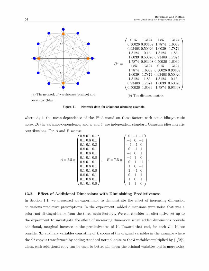
Bertsimas and Kallus:54 From Predictive to Prescriptive Analytics
Ê
Ê
ÊÊ
Ê
Ê
Ê
Ê
ÊÊ
Ê
Ê
‡
‡
‡
‡
-1.0 -0.5 0.5 1.0
-1.0
-0.5
0.5
1.0
(a) The network of warehouses (orange) and
locations (blue).
DT =
0BBBBBBBBBBBBBBBBB@
0.15 1.3124 1.85 1.31240.50026 0.93408 1.7874 1.60390.93408 0.50026 1.6039 1.78741.3124 0.15 1.3124 1.851.6039 0.50026 0.93408 1.78741.7874 0.93408 0.50026 1.60391.85 1.3124 0.15 1.3124
1.7874 1.6039 0.50026 0.934081.6039 1.7874 0.93408 0.500261.3124 1.85 1.3124 0.150.93408 1.7874 1.6039 0.500260.50026 1.6039 1.7874 0.93408
1CCCCCCCCCCCCCCCCCA
(b) The distance matrix.
Figure 11 Network data for shipment planning example.
where Ai is the mean-dependence of the ith demand on these factors with some idiosyncratic
noise, Bi the variance-dependence, and ✏i and �i are independent standard Gaussian idiosyncratic
contributions. For A and B we use
A = 2.5⇥
0BBBBBBBBBBBBBBBBB@
0.8 0.1 0.10.1 0.8 0.10.1 0.1 0.80.8 0.1 0.10.1 0.8 0.10.1 0.1 0.80.8 0.1 0.10.1 0.8 0.10.1 0.1 0.80.8 0.1 0.10.1 0.8 0.10.1 0.1 0.8
1CCCCCCCCCCCCCCCCCA
, B = 7.5⇥
0BBBBBBBBBBBBBBBBB@
0 �1 �1�1 0 �1�1 �1 00 �1 1�1 0 1�1 1 00 1 �11 0 �11 �1 00 1 11 0 11 1 0
1CCCCCCCCCCCCCCCCCA
.
13.2. E↵ect of Additional Dimensions with Diminishing Predictiveness
In Section 1.1, we presented an experiment to demonstrate the e↵ect of increasing dimension
on various predictive prescriptions. In the experiment, added dimensions were noise that was a
priori not distinguishable from the three main features. We can consider an alternative set up to
the experiment to investigate the e↵ect of increasing dimension when added dimensions provide
additional, marginal increase in the predictiveness of Y . Toward that end, for each L 2 N, we
consider 3L auxiliary variables consisting of L copies of the original variables in the example where
the `th copy is transformed by adding standard normal noise to the 3 variables multiplied by (1/2)`.
Thus, each additional copy can be used to better pin down the original variables but is more noisy
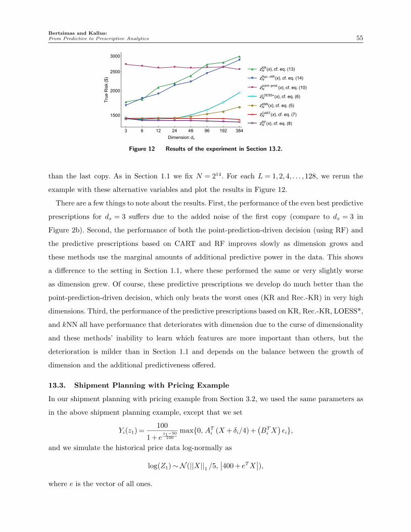
Bertsimas and Kallus:From Predictive to Prescriptive Analytics 55
▲ ▲
▲▲
▲
▲ ▲▲
▼▼
▼
▼▼
▼▼
▼■ ■ ■ ■ ■ ■ ■ ■
○ ○ ○ ○○
○
○
○
◆ ◆ ◆ ◆ ◆ ◆ ◆◆
◇ ◇ ◇ ◇ ◇ ◇ ◇ ◇□ □ □ □ □ □ □ □
3 6 12 24 48 96 192 384
1500
2000
2500
3000
Dimension dx
TrueRisk($)
▲ zNKR(x), cf. eq. (13)
▼ zNRec.-KR(x), cf. eq. (14)
■ zNpoint-pred.(x), cf. eq. (10)
○ zNLOESS*(x), cf. eq. (6)
◆ zNkNN(x), cf. eq. (5)
◇ zNCART(x), cf. eq. (7)
□ zNRF(x), cf. eq. (8)
Figure 12 Results of the experiment in Section 13.2.
than the last copy. As in Section 1.1 we fix N = 214. For each L = 1,2,4, . . . ,128, we rerun the
example with these alternative variables and plot the results in Figure 12.
There are a few things to note about the results. First, the performance of the even best predictive
prescriptions for dx = 3 su↵ers due to the added noise of the first copy (compare to dx = 3 in
Figure 2b). Second, the performance of both the point-prediction-driven decision (using RF) and
the predictive prescriptions based on CART and RF improves slowly as dimension grows and
these methods use the marginal amounts of additional predictive power in the data. This shows
a di↵erence to the setting in Section 1.1, where these performed the same or very slightly worse
as dimension grew. Of course, these predictive prescriptions we develop do much better than the
point-prediction-driven decision, which only beats the worst ones (KR and Rec.-KR) in very high
dimensions. Third, the performance of the predictive prescriptions based on KR, Rec.-KR, LOESS*,
and kNN all have performance that deteriorates with dimension due to the curse of dimensionality
and these methods’ inability to learn which features are more important than others, but the
deterioration is milder than in Section 1.1 and depends on the balance between the growth of
dimension and the additional predictiveness o↵ered.
13.3. Shipment Planning with Pricing Example
In our shipment planning with pricing example from Section 3.2, we used the same parameters as
in the above shipment planning example, except that we set
Yi(z1) =100
1+ ez1�50100
max{0, ATi (X + �i/4) +
�BT
i X�✏i},
and we simulate the historical price data log-normally as
log(Z1)⇠N (||X||1 /5,��400+ eT X
��),
where e is the vector of all ones.
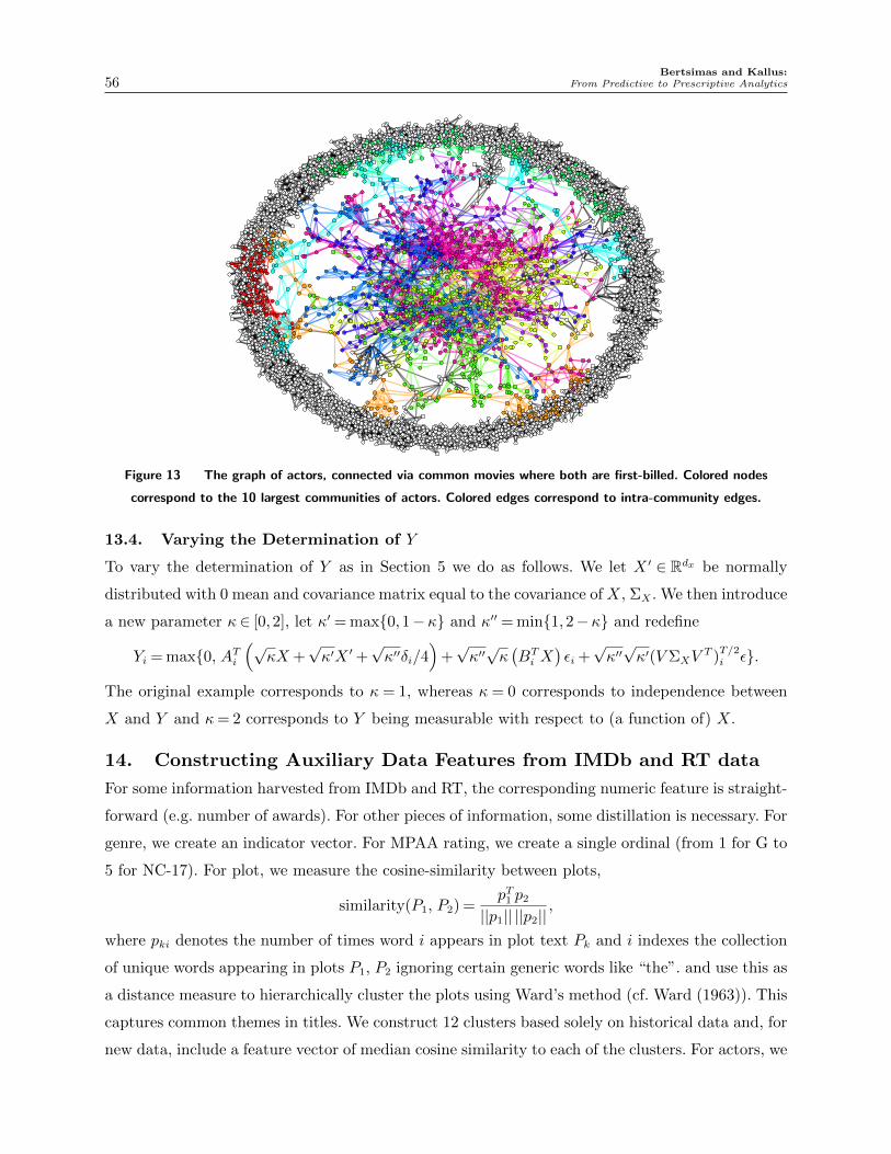
Bertsimas and Kallus:56 From Predictive to Prescriptive Analytics
Figure 13 The graph of actors, connected via common movies where both are first-billed. Colored nodes
correspond to the 10 largest communities of actors. Colored edges correspond to intra-community edges.
13.4. Varying the Determination of Y
To vary the determination of Y as in Section 5 we do as follows. We let X 0 2 Rdx be normally
distributed with 0 mean and covariance matrix equal to the covariance of X, ⌃X . We then introduce
a new parameter 2 [0,2], let 0 = max{0,1�} and 00 = min{1,2�} and redefine
Yi = max{0, ATi
⇣pX +
p0X 0 +
p00�i/4
⌘+p00p
�BT
i X�✏i +
p00
p0(V ⌃XV T )
T/2i ✏}.
The original example corresponds to = 1, whereas = 0 corresponds to independence between
X and Y and = 2 corresponds to Y being measurable with respect to (a function of) X.
14. Constructing Auxiliary Data Features from IMDb and RT data
For some information harvested from IMDb and RT, the corresponding numeric feature is straight-
forward (e.g. number of awards). For other pieces of information, some distillation is necessary. For
genre, we create an indicator vector. For MPAA rating, we create a single ordinal (from 1 for G to
5 for NC-17). For plot, we measure the cosine-similarity between plots,
similarity(P1, P2) =pT
1 p2
||p1|| ||p2||,
where pki denotes the number of times word i appears in plot text Pk and i indexes the collection
of unique words appearing in plots P1, P2 ignoring certain generic words like “the”. and use this as
a distance measure to hierarchically cluster the plots using Ward’s method (cf. Ward (1963)). This
captures common themes in titles. We construct 12 clusters based solely on historical data and, for
new data, include a feature vector of median cosine similarity to each of the clusters. For actors, we

Bertsimas and Kallus:From Predictive to Prescriptive Analytics 57
create a graph with titles as nodes and with edges between titles that share actors, weighted by the
number of actors shared. We use the method of Blondel et al. (2008) to find communities of titles
and create an actor-counter vector for memberships in the 10 largest communities (see Figure 13).
This approach is motivated by the existence of such actor groups as the “Rat Pack” (Humphery
Bogart and friends), “Brat Pack” (Molly Ringwald and friends), and “Frat Pack” (Owen Wilson
and friends) that often co-star in titles with a similar theme, style, and target audience.