frictional property of flexible element - intech -...

12

Frictional Property of Flexible Element

Keiji Imado Oita University

Japan

1. Introduction

In the calculation of frictional force of a flexible element such as a belt, rope or cable

wrapped around the cylinder, the famous Euler's belt formula (Hashimoto, 2006) or simply

known as the belt friction equation (Joseph F. Shelley, 1990) is used. The formula is useful

for designing a belt drive or band brake (J. A. Williams, 1994). On the other hand, a belt or

rope is conveniently used to tighten a luggage to a carrier or lift up the luggage from the

carrier. In that case, for the sake of adjusting the belt length and keeping an appropriate

tension during transportation, various kinds of belt buckles are used. These belt buckles

have been devised empirically and there was no theory about why it can fix the belt. The

first purpose of this chapter is to present the theory of belt buckle clearly by considering the

self-locking mechanism generated by wrapping the belt on the belt. Making use of the belt

tension for a locking mechanism, a belt buckle with no locking mechanism can be made. The

principle and some basic property of this new belt buckle are also shown.

The self-locking of belt may occur even in the case where a belt is wrapped on an axis two or

more times. The second purpose of this chapter is to present the frictional property of belt

wrapped on an axis two and three times through deriving the formulas corresponding to an

each condition. Making use of this self-locking property of belt, a belt-type one-way clutch

can be made (Imado, 2010). The principle and fundamental property of this new clutch are

described.

As the last part of this chapter, the frictional property of flexible element wrapped on a hard body with any contour is discussed. The frictional force can be calculated by the curvilinear integral of the curvature with respect to line element along the contact curve.

2. Theory of belt buckle

Notation C Magnification factor of belt tension F Frictional force, N Fij = Fji Frictional force between point Pi and Pj , N L Distance between two cylinder centers, m N Normal force of belt to surface, N Nij= Nji Normal force of belt between point Pi and Pj , N Pi Boundary of contact angle R Radius of main cylinder, m

www.intechopen.com

New Tribological Ways

236

Ti Tension of belt in i’th interval, N r Radius of accompanied cylinder, m μ Coefficient of friction for belt-cylinder contact μb Coefficient of friction for belt-belt contact θ Angle

θi Angle of point Pi

θij =θji Contact angle between Pi and Pj

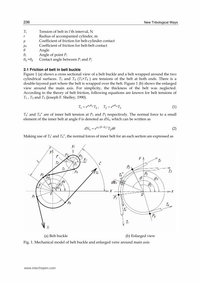
2.1 Friction of belt in belt buckle Figure 1 (a) shows a cross sectional view of a belt buckle and a belt wrapped around the two cylindrical surfaces. T1 and T4 (T1>T4 ) are tensions of the belt at both ends. There is a double-layered part where the belt is wrapped over the belt. Figure 1 (b) shows the enlarged view around the main axis. For simplicity, the thickness of the belt was neglected. According to the theory of belt friction, following equations are known for belt tensions of T1 , T2 and T3 (Joseph F. Shelley, 1990).

12 341 2 2 3,bT e T T e Tμ θ μθ= = (1)

T4’ and T4” are of inner belt tension at P1 and P2 respectively. The normal force to a small element of the inner belt at angle θ is denoted as dNb, which can be written as

2( )2

bbdN e T dμ θ θ θ−= (2)

Making use of T4’ and T4”, the normal forces of inner belt for an each section are expressed as

(a) Belt buckle (b) Enlarged view

Fig. 1. Mechanical model of belt buckle and enlarged veiw around main axis

www.intechopen.com


237

2

1

6

( )25 4

( )12 4

( )16 4

"

'

dN e T d

dN e T d

dN e T d

μ θ θμ θ θμ θ θ

θθθ

−−−

⎫= ⎪⎪= ⎬⎪= ⎪⎭ (3)

The frictional force between P1 and P6 is

6

16

116 16 4( 1)F dN e T

θ μθθ μ= = −∫ (4)

The inner belt tension T4’ is the sum of the frictional force F16 and the belt tension T4.

164 4 16 4'T T F e Tμθ= + = (5)

The frictional force F12 acting on the inner belt is composed of two forces denoted as F12in and F12out. The frictional force F12in is acting on the cylindrical surface, which is generated by the normal forces dNb and dN12. The normal force dNb is exerted from the outer belt. The other normal force dN12 is generated by the inner belt tension. So, F12in is given by

1 1

12 12

2 2

212 12 4( 1) ( 1) 'b

in bb

TF dN dN e e T

θ θ μ θ μθθ θ

μμ μ μ= + = − + −∫ ∫ (6)

Making use of Eq. (2), the frictional force F12out acting on the belt-belt boundary can be written as

1

12

212 2( 1)b

out b bF dN e Tθ μ θθ μ= = −∫ (7)

The frictional force F12 is the sum of Eqs. (6) and (7).

12 1212 2 4( 1) 1 ( 1) 'b

b

F e T e Tμ θ μθμμ

⎛ ⎞= − + + −⎜ ⎟⎝ ⎠ (8)

As the belt tension T4” is the sum of F12 and T4’ , making use of Eq. (5) and (8), T4” can be written as

26 124 12 4 4 2" ' ( 1) 1b

b

T F T e T e Tμθ μ θ μμ

⎛ ⎞= + = + − +⎜ ⎟⎝ ⎠ (9)

Making use of Eq. (3), the frictional force F25 can be written as

2

25

525 25 4( 1) "F dN e T

θ μθθ μ= = −∫ (10)

As the belt tension T3 is the sum of F25 and T4”, making use of Eqs. (9) and (10), T3 can be expressed as

25 26 123 25 4 4 2" ( 1) 1b

b

T F T e e T e Tμθ μθ μ θ μμ

⎧ ⎫⎛ ⎞⎪ ⎪= + = + − +⎜ ⎟⎨ ⎬⎪ ⎪⎝ ⎠⎩ ⎭ (11)

www.intechopen.com


238

Substituting Eq. (1) into Eq. (11) to eliminate T2 gives

( )56

1234 253 4( )1 ( 1) 1 /b

b

eT T

e e

μθμ θμ θ θ μ μ+= − − + (12)

Substituting Eq. (1) into Eq. (12) to get the relation between T1 and T4 gives

( )12 34 56

1234 25

( )

1 4( )1 ( 1) 1 /

b

bb

e eT T

e e

μ θ μ θ θμ θμ θ θ μ μ

++= − − + (13)

In the same manner from Eq. (1) to Eq. (13), in the case of T1<T4, corresponding relation of Eq. (13) yields as

34 56 12 16 12( )4 1( 1) 1b b

b

T e e e e Tμ θ θ μ θ μθ μ θ μμ+⎧ ⎫⎛ ⎞⎪ ⎪= + − +⎜ ⎟⎨ ⎬⎪ ⎪⎝ ⎠⎩ ⎭

(14)

2.2 Property of formulas of belt buckle The validity of Eqs. (13) and (14) might be checked by supposing an extreme case of either μ=0 or μb=0. Substituting μ=0 into Eq. (13) gives

12

121 4

2

b

b

eT T

e

μ θμ θ= − (15)

Next, substituting μb=0 into Eq. (13) gives

34 56

34 56

34 25

( )( )

1 4 4( )121

eT T C e T

e

μ θ θ μ θ θμ θ θθ μ+ ++= =− (16)

Substituting μb=0 into Eq. (15) or substituting μ=0 into Eq. (16) gives T1=T4. Substituting

12 0θ = into Eq. (13) to remove the double-layered segment on the ratio of belt tension yields

the conventional equation of belt friction.

34 56( )1 4T e Tμ θ θ+= (17)

Equation (17) is also obtained by substituting 12 0θ = into Eq. (16). This means that the ratio

of belt tension is magnified by the factor C

34 25( )

12

1

1C

eμ θ θθ μ += − (18)

due to the double-layered segment even in the case of μb=0. As far as these inspections are

concerned, there is no contradiction in Eq. (13). As Eqs. (13), (15) and (16) are of fractions,

the factor of T4 might become infinity meaning T4/T1=0. This fact virtually implies the

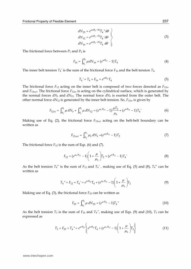
occurrence of self-locking. Figure 2 shows the relation of μb and θ12 satisfying b 12 2eμ θ = in

Eq. (15). Self-locking occurs in the region above this curve where b 12 2eμ θ > . On the other

hand, in the region below this curve, self-locking does not occur. In the case of μ=0, the

equilibrium of moment of belt tension about O in Fig. 1 gives

www.intechopen.com


239

0.20 0.25 0.30 0.35 0.40 0.45 0.5060

90

120

150

180

210

b 12e 2μ θ =

Sliding condition

Overl

appin

g a

ngle

of belt θ 12

, d

eg

Coefficient of belt-belt friction μb

Locking condition

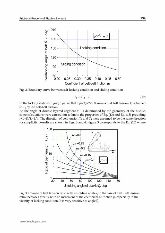
Fig. 2. Boundary curve between self-locking condition and sliding condition

4 2 12T T T= − (19)

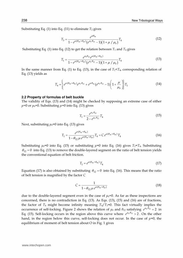
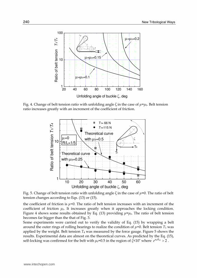
In the locking state with μ=0, T4=0 so that T1=2T2=2T3. It means that belt tension T1 is halved to T2 by the belt-belt friction. As the angle of double-layered segment θ12 is determined by the geometry of the buckle, some calculations were carried out to know the properties of Eq. (13) and Eq. (15) providing r/L=R/L=1/4. The direction of belt tension T1 and T4 were assumed to be the same direction for simplicity. Results are shown in Figs. 3 and 4. Figure 3 corresponds to the Eq. (15) where

20 40 60 80 100 120 140 1601

10

100

μb =0.1

μb =0.2

μb =0.25x

y

ζ

T 4

T1

Ra

tio

of

be

lt t

en

sio

n

T1/T

4

Unfolding angle of buckle ζ, deg

μb =0.3

μ =0

μb =0.15

Fig. 3. Change of belt tension ratio with unfolding angle ζ in the case of μ=0. Belt tension ratio increases greatly with an increment of the coefficient of friction μb especially in the vicinity of locking condition. It is very sensitive to angle ζ.

www.intechopen.com


240

20 40 60 80 100 120 140 1601

10

100

x

y

ζ

T 4

T1

μ=μb=0.1

μ=μb=0.15

μ=μb=0.2

Ratio

of b

elt t

en

sio

n T

1/T

4


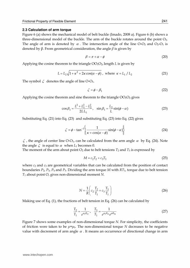
Fig. 4. Change of belt tension ratio with unfolding angle ζ in the case of μ=μb. Belt tension ratio increases greatly with an increment of the coefficient of friction.

10 20 30 40 50 601

10

T1= 66 N

T1=115 N

ζT4

T1

Theoretical curve

with μb=0.5

Ra

tio

of

be

lt t

en

sio

n T

1/ T

4


Theoretical curve

with μb=0.25

μ=0

R/L=1/5

Fig. 5. Change of belt tension ratio with unfolding angle ζ in the case of μ=0. The ratio of belt tension changes according to Eqs. (13) or (15).

the coefficient of friction is μ=0. The ratio of belt tension increases with an increment of the coefficient of friction μb. It increases greatly when it approaches the locking condition. Figure 4 shows some results obtained by Eq. (13) providing μ=μb. The ratio of belt tension becomes far bigger than the that of Fig. 3. Some experiments were carried out to verify the validity of Eq. (15) by wrapping a belt around the outer rings of rolling bearings to realize the condition of μ=0. Belt tension T1 was applied by the weight. Belt tension T4 was measured by the force gauge. Figure 5 shows the results. Experimental data are almost on the theoretical curves. As predicted by the Eq. (15), self-locking was confirmed for the belt with μb=0.5 in the region of ζ<10˚ where 12 2beμ θ > .

www.intechopen.com


241

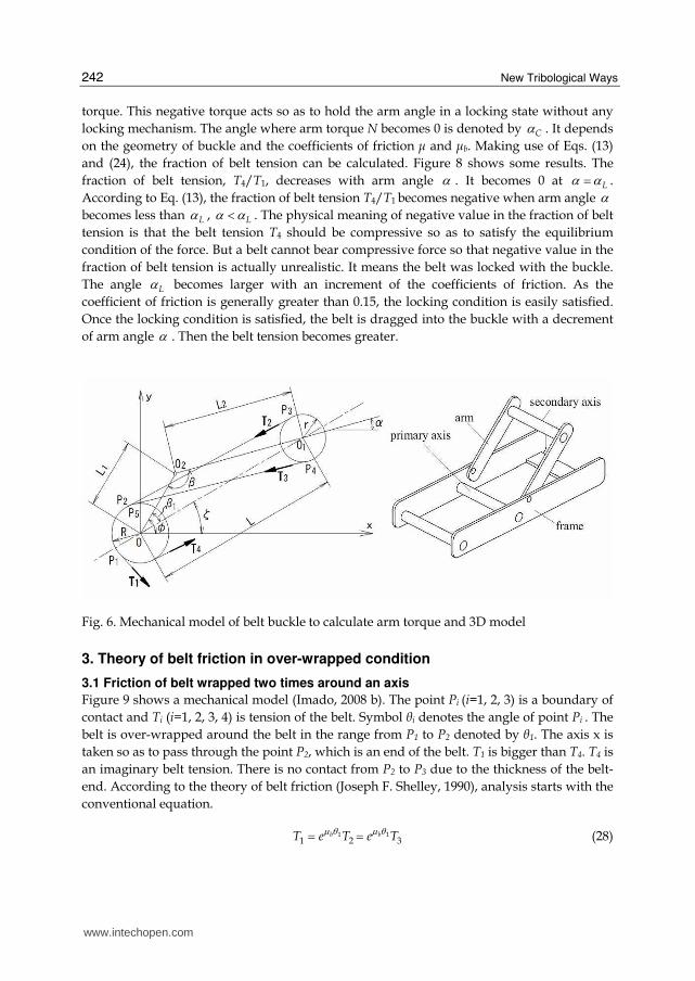
2.3 Calculation of arm torque

Figure 6 (a) shows the mechanical model of belt buckle (Imado, 2008 a). Figure 6 (b) shows a

three-dimensional model of the buckle. The arm of the buckle rotates around the point O2.

The angle of arm is denoted by α . The intersection angle of the line O-O2 and O2-O1 is

denoted by β. From geometrical consideration, the angle ┚ is given by

β π α φ= + − (20)

Applying the cosine theorem to the triangle OO1O2, length L is given by

22 1 2 cos( )L L κ κ α φ= + + − , where 1 2/L Lκ = (21)

The symbol ζ denotes the angle of line O-O1.

1ζ φ β= − (22)

Applying the cosine theorem and sine theorem to the triangle OO1O2 gives

2 2 2

1 2 21 1

1

cos , sin sin( )2

L L L L

LL Lβ β φ α+ −= = − (23)

Substituting Eq. (21) into Eq. (23) and substituting Eq. (23) into Eq. (22) gives

1 1tan sin( )

cos( )ζ φ φ ακ α φ− ⎧ ⎫⎪ ⎪= − −⎨ ⎬+ −⎪ ⎪⎩ ⎭ (24)

ζ , the angle of center line O-O1, can be calculated from the arm angle α by Eq. (24). Note

the angle ζ is equal to α when L1 becomes 0. The moment of the arm about point O2 due to belt tensions T2 and T3 is expressed by

2 2 3 3M c T c T= + (25)

where c2 and c3 are geometrical variables that can be calculated from the position of contact

boundaries P2, P3, P4 and P5. Dividing the arm torque M with RT1, torque due to belt tension

T1 about point O, gives non-dimensional moment N.

322 3

1 1

1 TTN c c

R T T

⎛ ⎞= +⎜ ⎟⎝ ⎠ (26)

Making use of Eq. (1), the fractions of belt tension in Eq. (26) can be calculated by

12 12 34

32

1 1

1 1,

b b

TT

T Te e eμ θ μ θ μθ= = (27)

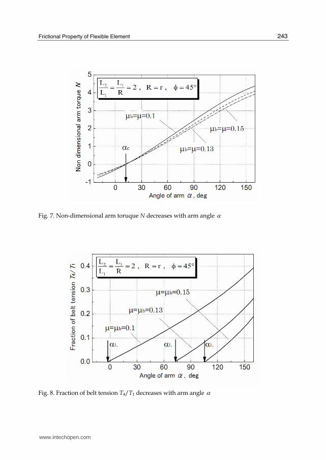
Figure 7 shows some examples of non-dimensional torque N. For simplicity, the coefficients

of friction were taken to be μ=μb. The non-dimensional torque N decreases to be negative

value with decrement of arm angle α . It means an occurrence of directional change in arm

www.intechopen.com


242

torque. This negative torque acts so as to hold the arm angle in a locking state without any

locking mechanism. The angle where arm torque N becomes 0 is denoted by Cα . It depends

on the geometry of buckle and the coefficients of friction μ and μb. Making use of Eqs. (13)

and (24), the fraction of belt tension can be calculated. Figure 8 shows some results. The

fraction of belt tension, T4/T1, decreases with arm angle α . It becomes 0 at Lα α= .

According to Eq. (13), the fraction of belt tension T4/T1 becomes negative when arm angle α

becomes less than Lα , Lα α< . The physical meaning of negative value in the fraction of belt

tension is that the belt tension T4 should be compressive so as to satisfy the equilibrium

condition of the force. But a belt cannot bear compressive force so that negative value in the

fraction of belt tension is actually unrealistic. It means the belt was locked with the buckle.

The angle Lα becomes larger with an increment of the coefficients of friction. As the

coefficient of friction is generally greater than 0.15, the locking condition is easily satisfied.

Once the locking condition is satisfied, the belt is dragged into the buckle with a decrement

of arm angle α . Then the belt tension becomes greater.

Fig. 6. Mechanical model of belt buckle to calculate arm torque and 3D model

3. Theory of belt friction in over-wrapped condition

3.1 Friction of belt wrapped two times around an axis

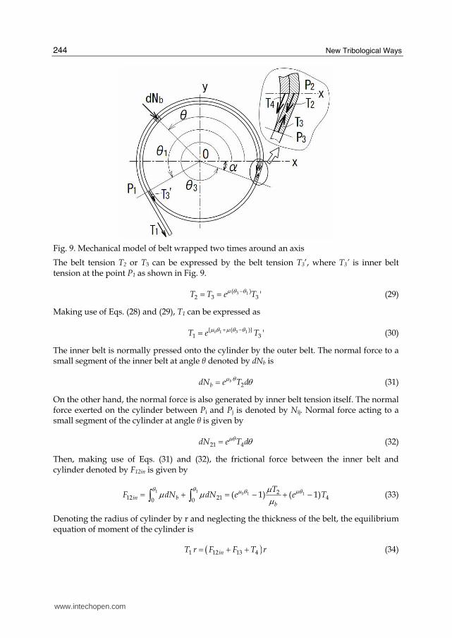
Figure 9 shows a mechanical model (Imado, 2008 b). The point Pi (i=1, 2, 3) is a boundary of

contact and Ti (i=1, 2, 3, 4) is tension of the belt. Symbol θi denotes the angle of point Pi . The

belt is over-wrapped around the belt in the range from P1 to P2 denoted by θ1. The axis x is

taken so as to pass through the point P2, which is an end of the belt. T1 is bigger than T4. T4 is

an imaginary belt tension. There is no contact from P2 to P3 due to the thickness of the belt-

end. According to the theory of belt friction (Joseph F. Shelley, 1990), analysis starts with the

conventional equation.

1 11 2 3

b bT e T e Tμ θ μ θ= = (28)

www.intechopen.com


243

Fig. 7. Non-dimensional arm toruque N decreases with arm angle α

Fig. 8. Fraction of belt tension T4/T1 decreases with arm angle α

www.intechopen.com


244

Fig. 9. Mechanical model of belt wrapped two times around an axis

The belt tension T2 or T3 can be expressed by the belt tension T3’, where T3’ is inner belt tension at the point P1 as shown in Fig. 9.

3 1( )2 3 3 'T T e Tμ θ θ−= = (29)

Making use of Eqs. (28) and (29), T1 can be expressed as

1 3 1{ ( )}1 3 'bT e Tμ θ μ θ θ+ −= (30)

The inner belt is normally pressed onto the cylinder by the outer belt. The normal force to a small segment of the inner belt at angle θ denoted by dNb is

2b

bdN e T dμ θ θ= (31)

On the other hand, the normal force is also generated by inner belt tension itself. The normal force exerted on the cylinder between Pi and Pj is denoted by Nij. Normal force acting to a small segment of the cylinder at angle θ is given by

21 4dN e T dμθ θ= (32)

Then, making use of Eqs. (31) and (32), the frictional force between the inner belt and cylinder denoted by F12in is given by

1 1

1 1212 21 40 0

( 1) ( 1)bin b

b

TF dN dN e e T

θ θ μ θ μθμμ μ μ= + = − + −∫ ∫ (33)

Denoting the radius of cylinder by r and neglecting the thickness of the belt, the equilibrium equation of moment of the cylinder is

( )1 12 13 4inT r F F T r= + + (34)

www.intechopen.com


245

Here, the frictional force F13 exerted on the surface between P1 and P3 is given by

3

3 11

1

( )( )13 3 3' { 1} 'F e T d e T

θ μ θ θμ θ θθμ θ −−= = −∫ (35)

Substituting Eqs. (33) and (35) into Eq. (34) gives

1 3 1 1( )21 3 4( 1) { 1} 'b

b

TT e e T e Tμ θ μ θ θ μθμ

μ −= − + − + (36)

Substituting T2 and T3’ in Eq. (36) as functions of T1 by making use of Eqs. (28) and (30) gives

1

1 3 1

( )

1 4( )

(1 ) 1

b

b

b

eT T

e e

θ μ μμ θ μ θ θμ

μ

+− −

= ⎛ ⎞− − +⎜ ⎟⎝ ⎠ (37)

This is the targeted equation that expresses the relation between T1 and T4. Equation (37) can be checked by supposing an extreme case of either μ=0 or μb=0. Substituting μ=0 into Eq. (37) gives T1=T4 as a matter of course. Substituting of μb=0 into Eq. (37) requires limiting operation.

1

10

lim (1 )b

b b

eμ θ

μμ μθμ→ − = − (38)

Making use of Eq. (38), Eq. (37) becomes Eq. (39) for the case of μb=0.

1

3 11 4( )

1

eT T

e

μθμ θ θμθ − −= − + (39)

Equation (39) implies the belt may be locked firmly around an axis when the denominator of the fraction in Eq. (39) becomes 0. Substituting μ=0 into Eq. (39) gives T1=T4 again as a matter of course. Substituting μ=μb into Eq. (37) gives

1 3( )1 4T e T

μ θ θ+= (40)

Equation (40) is exactly the same form as the Euler’s belt formula though was derived from the expression that took an effect of over-wrapping of belt into account. Equation (40) implies that the belt cannot be locked on the cylinder as far as the wrapping angle is finite. Letting θ1=0 in Eq. (37) to eliminate the over-wrapping part gives

3

1 4T e Tμθ= (41)

This is the well-known Euler’s belt formula. So the Euler’s belt formula was proved to be included as a special case in Eq. (37). Equation (41) can also be obtained from Eqs. (39) and (40). Next, let’s consider some locking conditions. According to Eq. (37), the belt tension ratio T4 /T1 can be expressed as

www.intechopen.com


246

1 3 1

1 1

( )

4( ) ( )

1

(1 ) 1b

b b

b

e eT

T ee

μ θ μ θ θ

θ μ μ θ μ μ

μμ − −

+ +

⎛ ⎞− − +⎜ ⎟ Γ⎝ ⎠= = (42)

The locking condition is satisfied when the numerator of Eq. (42) becomes 0 meaning T4 =0. So, the discriminant of locking condition can be expressed as

1 3 1( )1(1 ) 1e eκμθ μ θ θκ − −⎛ ⎞Γ = − − +⎜ ⎟⎝ ⎠ (43)

Locking condition is satisfied in the case of Γ≤0. Critical point is Γ=0. Here, κ denotes a ratio of the coefficient of friction.

/bκ μ μ= (44)

As 1 1eκμθ ≥ and 3 1( ) 0e μ θ θ− − > , κ should be less than unity to make the value of locking

discriminant of Eq. (43) be Γ<0. As can be seen in Fig. 9, the angle θ3 is smaller than 2π due to

the thickness of the belt. From geometrical consideration in Fig. 9, following equation is

obtained.

cos 1r t

r t rα = ≈ −+ (45)

Here, t is thickness of the belt and r is a radius of the cylinder. When angle α is small, the

angle α can be roughly estimated by

2 /t rα ≈ (46)

Supposing the angle of non-contact is α =15˚, the corresponding critical locking condition

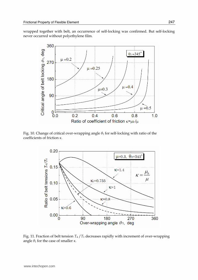
can be evaluated by solving Eq. (43). Figure 10 shows some solutions. The critical angle of

belt locking θ1 decreases with an increment of the coefficient of friction μ. Provided the

coefficient of friction is constant, the critical angle of belt locking θ1 increases with an

increment of κ. This fact means that the belt is likely to lock with a decrement of κ. So the

smaller coefficient of friction μb is preferable for self-locking. The limiting condition for the

belt locking is κ =0 or μb=0.

Figure 11 illustrates the effect of κ on the fraction of belt tension T4 /T1 for the case of μ=0.3

and θ3=345°. Making use of Eq. (41), the convergence point is calculated. It is T4 /T1 =exp(-

μθ3)≈0.164. It is clear that the fraction of belt tension T4 /T1 is greatly influenced by the

magnitude of κ, μb /μ. The belt tension ratio T4 /T1 decreases with an increment of over-

wrapping angle θ1 except for the case of κ=1.4. When 1κ ≥ , the fraction of belt tension is

always positive, so that the self-locking never occurs. Provided θ1=360°, θ3=345° and μ=0.3,

the critical ratio of the coefficient of friction κc for the self-locking with two times over-

wrapping condition was calculated by using the discriminant Eq. (43). It was κc=0.735. The

corresponding line was plotted with a dashed line in Fig. 11. The magnitude of κ should be

smaller than κc to cause the self-locking. Figure 12 shows a method by which the coefficient of friction between the belt and belt can be reduced so as to satisfy the self-locking condition. When a polyethylene film was

www.intechopen.com


247

wrapped together with belt, an occurrence of self-locking was confirmed. But self-locking never occurred without polyethylene film.

Fig. 10. Change of critical over-wrapping angle θ1 for self-locking with ratio of the coefficients of friction κ.

Fig. 11. Fraction of belt tension T4 /T1 decreases rapidly with increment of over-wrapping angle θ1 for the case of smaller κ.

www.intechopen.com


248

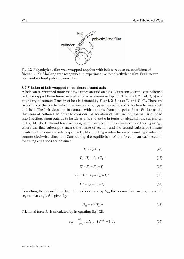
Fig. 12. Polyethylene film was wrapped together with belt to reduce the coefficient of friction μb. Self-locking was recognized in experiment with polyethylene film. But it never occurred without polyethylene film.

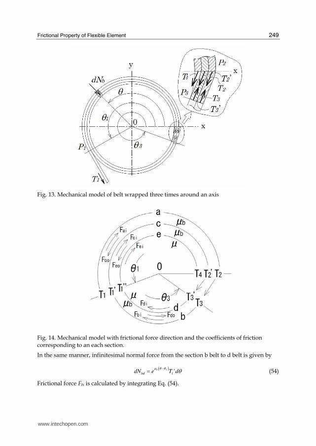
3.2 Friction of belt wrapped three times around axis A belt can be wrapped more than two times around an axis. Let us consider the case where a

belt is wrapped three times around an axis as shown in Fig. 13. The point Pi (i=1, 2, 3) is a

boundary of contact. Tension of belt is denoted by Ti (i=1, 2, 3, 4) or Ti’ and T1>T4. There are

two kinds of the coefficients of friction μ and μb. μb is the coefficient of friction between belt

and belt. The belt does not in contact with the axis from the point P2 to P3 due to the

thickness of belt-end. In order to consider the equation of belt friction, the belt is divided

into 5 sections from outside to inside as a, b, c, d and e in terms of frictional force as shown

in Fig. 14. The frictional force working on an each section is expressed by either Fsi or Fso ,

where the first subscript s means the name of section and the second subscript i means

inside and o means outside respectively. Note that Fsi works clockwisely and Fso works in a

counter-clockwise direction. Considering the equilibrium of the force in an each section,

following equations are obtained.

1 2aiT F T= + (47)

3 2 1 'biT T F T= = + (48)

1 2' '

ci coT F F T= − + (49)

3 2 1' ' "di doT T F F T= = − + (50)

1 4" ei eoT F F T= − + (51)

Denothing the normal force from the section a to c by Nac, the normal force acting to a small

segment at angle θ is given by

2b

acdN e T dμ θ θ= (52)

Frictional force Fai is calculated by integrating Eq. (52).

( )11

201b

ai b acF dN e Tθ μ θθ μ== = −∫ (53)

www.intechopen.com


249

Fig. 13. Mechanical model of belt wrapped three times around an axis

Fig. 14. Mechanical model with frictional force direction and the coefficients of friction corresponding to an each section.

In the same manner, infinitesimal normal force from the section b belt to d belt is given by

( )1

1'

μ θ θ θ−= b

bddN e T d (54)

Frictional force Fbi is calculated by integrating Eq. (54).

www.intechopen.com


250

( ) ( )( )3 3 1 3 1

1 1

1 1' 1 '

θ θ μ θ θ μ θ θθ θμ μ θ− −= = = −∫ ∫ b b

bi b bd bF dN e T d e T (55)

Making use of Eq. (52), infinitesimal normal force from section c belt to e belt is given by

2 2 2' 'b b bce acdN e T d dN e T d e T dμ θ μ θ μ θθ θ θ= + = + (56)

Frictional force Fci is calculated by integrating Eq. (56).

( ) ( )( )1 11

2 2 2 20 0' 1 'b b

ci b ce bF dN e T T d e T Tθ θ μ θ μ θμ μ θ= = + = − +∫ ∫ (57)

Making use of Eq. (54), infinitesimal normal force from section d belt to the axis is given by

( ) ( ) ( )1 1 1

1 1 1" " '

μ θ θ μ θ θ μ θ θθ θ θ− − −= + = + b

d bddN e T d dN e T d e T d (58)

Frictional force Fdi is calculated by integrating Eq. (58).

( ) ( )( ) ( )( ) ( )( )3 3 1 1 3 1 3 1

1 1

1 1 1 1" ' 1 " 1 '

θ θ μ θ θ μ θ θ μ θ θ μ θ θθ θ

μμ μ θ μ− − − −= = + = − + −∫ ∫ b b

di d

b

F dN e T e T d e T e T (59)

Making use of Eq. (56), infinitesimal normal force from section e belt to the axis is given by

4 4 2 2'b be cedN e T d dN e T d e T d e T dμ θ μ θμθ μθθ θ θ θ= + = + + (60)

Then, the frictional force Fei is given by

( ) ( ) ( )( )1 111

4 2 2 4 2 20 0' 1 1 'b b b

e i eb

F dN e T e T e T d e T e T Tθ θ μ θ μ θ μ θμθμθ μμ μ θ μ= = + + = − + − +∫ ∫ (61)

Neglecting the thickness of the belt, the equilibrium requirement of the moment gives

1 4d i e iT F F T= + + (62)


( )( ) ( )( ) ( )( )3 1 3 1 1 1

1 1 1 2 2 41 " 1 ' 1 '

μ θ θ μ θ θ μ θ μθμ μμ μ

− −= − + − + − + +b b

b b

T e T e T e T T e T (63)

The belt tensions T1’, T1”, T2 and T2’ in Eq. (63) should be expressed by the function of T4. From the law of action and reaction,

, ,= = =co ai eo ci do bi

F F F F F F (64)

Substituting Eqs. (53), (55), (57), (59) and (61) into Eqs. (47) to (51) give

11 2 2

baiT F T e Tμ θ= + = (65)

( )3 1

2 3 1 1' '

μ θ θ−= = + = b

biT T F T e T (66)

( )( ) ( )1 1 11 2 2 2 2 2 2' ' 1 ' 1 ' 'b b b

ci coT F F T e T T e T T e Tμ θ μ θ μ θ= − + = − + − − + = (67)

www.intechopen.com


251

( ) ( )( )3 1 3 1

3 2 1 1 1 1' ' " " " 1 1 '

μ θ θ μ θ θ μμ

− − ⎛ ⎞= = − + = − + = + − −⎜ ⎟⎝ ⎠b

di do di bi

b

T T F F T F F T e T e T (68)

( ) ( )1 11 4 2 2 4" 1 1 'b

ei eob

T F F T e T T e Tμ θ μθμμ

⎛ ⎞= − + = − − + +⎜ ⎟⎝ ⎠ (69)

Making use of Eqs. (65), (66) and (67) gives,

( ) ( )1 3 1 3

1 2 3' '

μ θ θ μ θ θ+ += =b b

T e T e T (70)

Substituting Eq. (68) into Eq. (70) and making use of Eq. (67) gives

( ) ( ) ( )( )1 3 3 1 3 1 1

1 1 2" 1 1 '

μ θ θ μ θ θ μ θ θ μ θμμ

+ − −⎧ ⎫⎛ ⎞⎪ ⎪= + − −⎨ ⎜ ⎟ ⎬⎪ ⎪⎝ ⎠⎩ ⎭b b b

b

T e e T e e T (71)

Making use of Eqs. (65), (66) and (67) gives

( )1 3

1

2' μ θ θ+=

b

TT

e

(72)

Substituting Eq. (72) into Eq. (71) gives

( ) ( ) ( )( )1 3 3 1 3 11

1 1 1" 1 1

μ θ θ μ θ θ μ θ θμ θ μμ

+ + − − ⎛ ⎞= + − −⎜ ⎟⎝ ⎠b bb

b

T e T e e T (73)

Rearranging Eq. (73) gives,

( )( ) ( )3 1

1 3 3 11 1 1

1 1

"

μ θ μ θ

μ θ θ μ θ θ

μμ

+ + −

⎛ ⎞− − −⎜ ⎟⎝ ⎠= =b b

b

b

e e

T T AT

e

(74)

Making use of Eqs. (65) and (72) gives

( )3

1 32 2 1

1'

μ θμ θ θ+

++ = b

b

eT T T

e

(75)


( )( )

( )3 1

11

1 31 1 4 1 4

1 1" 1

μ θ μ θμθμθ

μ θ θμμ +

+ −⎛ ⎞= − + = +⎜ ⎟⎝ ⎠b b

b

b

e e

T T e T BT e T

e

(76)

Substituting Eq. (76) into the left hand side of Eq. (74) gives,

www.intechopen.com


252

( )( )( )

( )( ) ( )

"

μ θ μ θμθμθ

μ θ θ

μ θ μ θ

μ θ θ μ θ θ

μμ

μμ

+

+ + −

+ −⎛ ⎞= − + = +⎜ ⎟⎝ ⎠⎛ ⎞− − −⎜ ⎟⎝ ⎠= =

b 3 b 1

11

b 1 3

b 3 b 1

b 1 3 3 1

1 1 4 1 4

b

b

1 1

e 1 e 1

T 1 T e T BT e T

e

1 e e 1

T AT

e

(77)

Equation (77) can be written in the form of

1

1 4

eT T

A B

μθ= − (78)

where

( )

( ) ( )( )( )

( )3 1

3 1

1 3 3 1 1 3

1 11 1

, 1

μ θ μ θ μ θ μ θ

μ θ θ μ θ θ μ θ θ

μμ μ

μ+ + − +

⎛ ⎞− − −⎜ ⎟ + −⎛ ⎞⎝ ⎠= = −⎜ ⎟⎝ ⎠b b

b b

b b

b

b

e ee e

A B

e e

(79)

Eqs. (78) and (79) are the targeted equations that express the relation between T1 and T4 in the case of a belt wrapped three times around an axis .

3.3 Characteristics of belt friction equation with three times wrapping around axis The equation derived in the previous section seems complex. It can be checked by assuming some extreme cases such as μ=0, μb=0 and μ=μb. In the case of μ=0, Eq. (79) becomes,

( )

( )( )( )

( )3 1 3 1

1 3 1 3

1 1 1,

μ θ μ θ μ θ μ θμ θ θ μ θ θ+ +

+ − + −= = −b b b b

b b

e e e eA B

e e

(80)

then

( )( )

1 3

1 3

1

μ θ θμ θ θ

++− = =b

b

eA B

e

(81)

Substituting Eq. (81) and μ=0 into Eq. (78) gives T1=T4. In the case of μb=0, limiting operations are required. For the term A in Eq. (79),

( ) ( )3 1

3 10

limμ θ μ θ

μμ μ θ θμ→ − = −b b

bb

e e (82)

For the term B in Eq. (79),

( )( )3 1

10

lim 1 1 2μ θ μ θ

μμ μθμ→ + − =b b

bb

e e (83)

Then Eq. (79) becomes,

( )( )3 1

3 1

1

1, 2μ θ θ

μ θ θ μθ−− −= =A B

e

(84)

www.intechopen.com


253

Substituting Eq. (84) into (78) gives

( )( )3

3 11 4

3 1 11 2

μθμ θ θμ θ θ θ −= − − +

eT T

e

(85)

In order to consider the smallest wrapping angle of three times wrapping, substituting θ1=0

into Eq. (85) gives,

3

1 431

eT T

μθμθ= − (86)

On the other hand, substituting θ1=θ3 into Eq. (85) gives,

3

1 431 2

eT T

μθμθ= − (87)

Equation (87) shows the relation of belt tension with the largest wrapping angle of three

times wrapping. The locking condition is satisfied when the denominator of Eqs. (86) and

(87) become 0, so that in the case of θ1=θ3, only 1/2 of the coefficient of friction is required

for self locking in compared with the case of θ1=0.

In the case of μb=μ, Eq. (79) becomes,

32

1, 0μθ= =A B

e

(88)

so that Eq. (78) becomes,

( )1

1 32

1 4 4

μθ μ θ θ+= =−e

T T e TA B

(89)

Substituting θ1=0 into Eq. (89) gives,

321 4T e Tμθ= (90)

Substituting θ1=θ3 into Eq. (89) gives,

331 4T e Tμθ= (91)

Note the magnitude of the wrapping angle of Eqs. (90) and (91). They are exactly the same

form as the Euler’s belt formula though they were derived considering the effect of over-

wrapping of belt on belt friction.

Next, Substituting θ1=0 into Eq. (79) provided the boundary of two and three times over-

wrapping of belt gives,

( )

( )3

3

1 1 1

, 0

μ θ

θ μ μ

μμ

+

⎛ ⎞+ − −⎜ ⎟⎝ ⎠= =b

b

b

e

A B

e

(92)

www.intechopen.com


254

then Eq. (78) becomes

3

3

( )

1 4 4

1

(1 ) 1 1

b

b

b

eT T T

A Be

θ μ μμ θ μ

μ

+= =− ⎛ ⎞− − +⎜ ⎟⎝ ⎠ (93)

On the other hand, substituting θ1=θ3 into Eq. (37) in the section 3.1 that was the equation for two times over-wrapping conditions gives,

3

3

( )

1 4

(1 ) 1 1

b

b

b

eT T

e

θ μ μμ θ μ

μ

+= ⎛ ⎞− − +⎜ ⎟⎝ ⎠ (94)

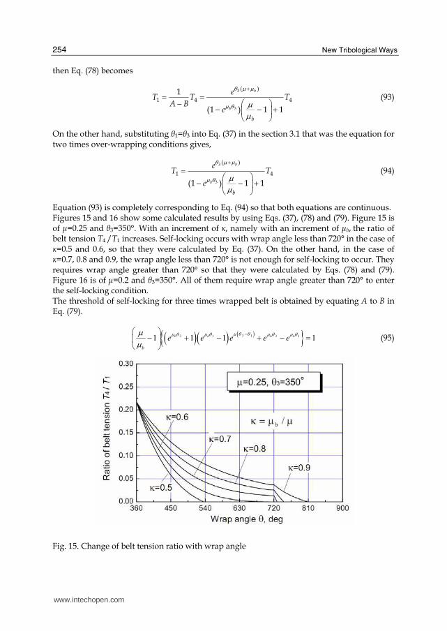
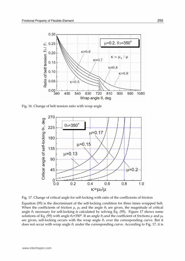
Equation (93) is completely corresponding to Eq. (94) so that both equations are continuous. Figures 15 and 16 show some calculated results by using Eqs. (37), (78) and (79). Figure 15 is of μ=0.25 and θ3=350°. With an increment of κ, namely with an increment of μb, the ratio of belt tension T4 /T1 increases. Self-locking occurs with wrap angle less than 720° in the case of κ=0.5 and 0.6, so that they were calculated by Eq. (37). On the other hand, in the case of κ=0.7, 0.8 and 0.9, the wrap angle less than 720° is not enough for self-locking to occur. They requires wrap angle greater than 720° so that they were calculated by Eqs. (78) and (79). Figure 16 is of μ=0.2 and θ3=350°. All of them require wrap angle greater than 720° to enter the self-locking condition. The threshold of self-locking for three times wrapped belt is obtained by equating A to B in Eq. (79).

( )( ) ( ){ }3 13 1 3 11 1 1 1μ θ θμ θ μ θ μ θ μ θμ

μ−⎛ ⎞− + − + − =⎜ ⎟⎝ ⎠

b b b b

b

e e e e e (95)

Fig. 15. Change of belt tension ratio with wrap angle

www.intechopen.com


255

Fig. 16. Change of belt tension ratio with wrap angle

Fig. 17. Change of critical angle for self-locking with ratio of the coefficients of friction

Equation (95) is the discriminant of the self-locking condition for three times wrapped belt. When the coefficients of friction μ, μb and the angle θ3 are given, the magnitude of critical angle θ1 necessary for self-locking is calculated by solving Eq. (95). Figure 17 shows some solutions of Eq. (95) with angle θ3=350°. If an angle θ3 and the coefficient of frictions μ and μb are given, self-locking occurs with the wrap angle θ1 over the corresponding curve. But it does not occur with wrap angle θ1 under the corresponding curve. According to Fig. 17, it is

www.intechopen.com


256

clearly seen that wrap angle θ1 becomes larger with an increment of κ. It also becomes larger with a decrement of the coefficient of friction μ. Provided κ is small enough, it is noticeable that the self-locking occurs theoretically even with these small coefficients of friction.

4. Novel clutch utilizing self-locking property of belt

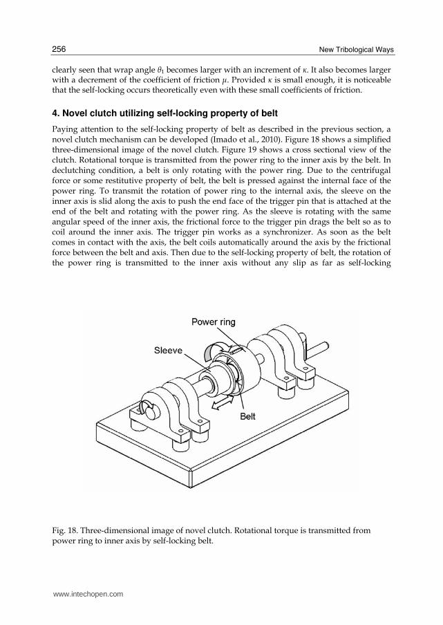
Paying attention to the self-locking property of belt as described in the previous section, a novel clutch mechanism can be developed (Imado et al., 2010). Figure 18 shows a simplified three-dimensional image of the novel clutch. Figure 19 shows a cross sectional view of the clutch. Rotational torque is transmitted from the power ring to the inner axis by the belt. In declutching condition, a belt is only rotating with the power ring. Due to the centrifugal force or some restitutive property of belt, the belt is pressed against the internal face of the power ring. To transmit the rotation of power ring to the internal axis, the sleeve on the inner axis is slid along the axis to push the end face of the trigger pin that is attached at the end of the belt and rotating with the power ring. As the sleeve is rotating with the same angular speed of the inner axis, the frictional force to the trigger pin drags the belt so as to coil around the inner axis. The trigger pin works as a synchronizer. As soon as the belt comes in contact with the axis, the belt coils automatically around the axis by the frictional force between the belt and axis. Then due to the self-locking property of belt, the rotation of the power ring is transmitted to the inner axis without any slip as far as self-locking

Fig. 18. Three-dimensional image of novel clutch. Rotational torque is transmitted from power ring to inner axis by self-locking belt.

www.intechopen.com


257

Trigger Pin

Belt

Sleeve

Power

Ring

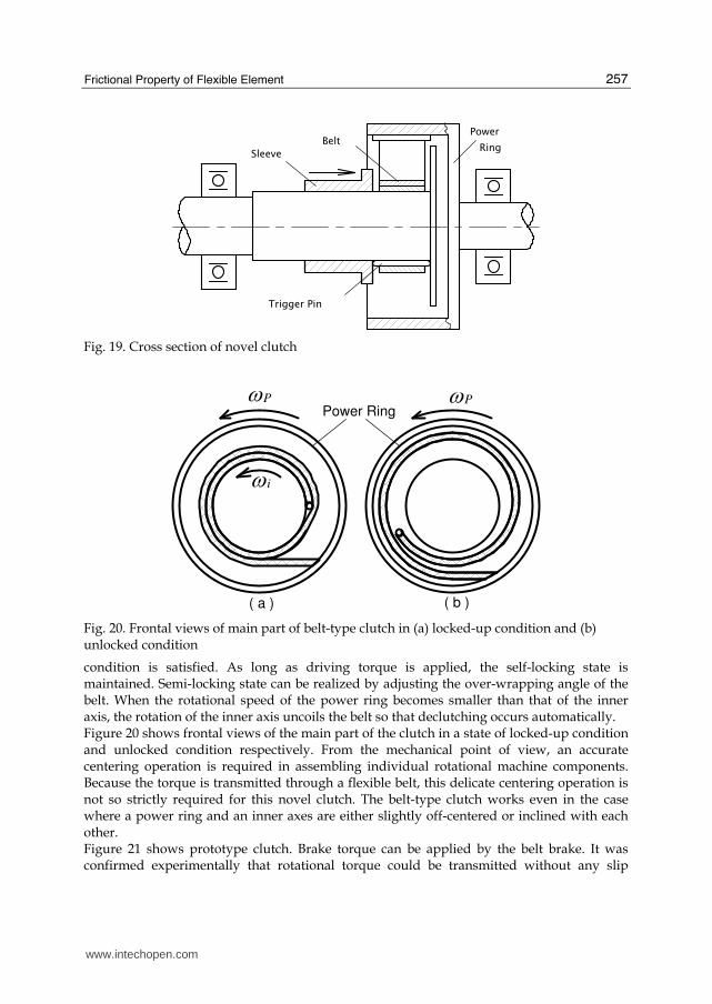
Fig. 19. Cross section of novel clutch

( a ) ( b )

Power RingωP ωP

ωi

Fig. 20. Frontal views of main part of belt-type clutch in (a) locked-up condition and (b) unlocked condition

condition is satisfied. As long as driving torque is applied, the self-locking state is maintained. Semi-locking state can be realized by adjusting the over-wrapping angle of the belt. When the rotational speed of the power ring becomes smaller than that of the inner axis, the rotation of the inner axis uncoils the belt so that declutching occurs automatically.

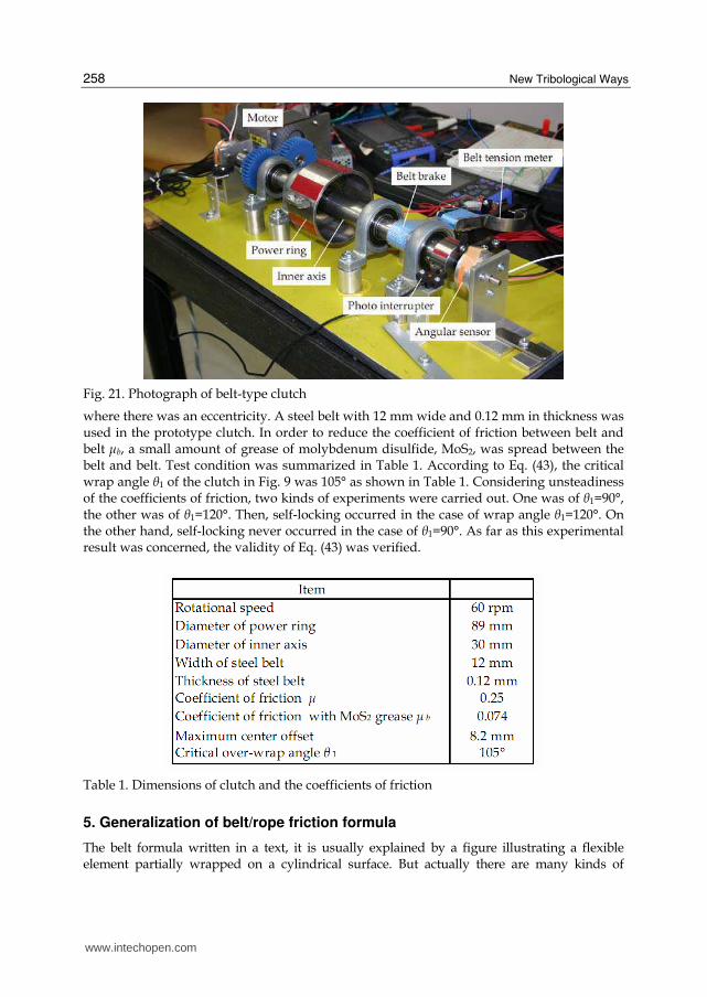
Figure 20 shows frontal views of the main part of the clutch in a state of locked-up condition and unlocked condition respectively. From the mechanical point of view, an accurate centering operation is required in assembling individual rotational machine components. Because the torque is transmitted through a flexible belt, this delicate centering operation is not so strictly required for this novel clutch. The belt-type clutch works even in the case where a power ring and an inner axes are either slightly off-centered or inclined with each other. Figure 21 shows prototype clutch. Brake torque can be applied by the belt brake. It was confirmed experimentally that rotational torque could be transmitted without any slip

www.intechopen.com


258

Fig. 21. Photograph of belt-type clutch

where there was an eccentricity. A steel belt with 12 mm wide and 0.12 mm in thickness was used in the prototype clutch. In order to reduce the coefficient of friction between belt and belt μb, a small amount of grease of molybdenum disulfide, MoS2, was spread between the belt and belt. Test condition was summarized in Table 1. According to Eq. (43), the critical wrap angle θ1 of the clutch in Fig. 9 was 105° as shown in Table 1. Considering unsteadiness of the coefficients of friction, two kinds of experiments were carried out. One was of θ1=90°, the other was of θ1=120°. Then, self-locking occurred in the case of wrap angle θ1=120°. On the other hand, self-locking never occurred in the case of θ1=90°. As far as this experimental result was concerned, the validity of Eq. (43) was verified.

Table 1. Dimensions of clutch and the coefficients of friction

5. Generalization of belt/rope friction formula

The belt formula written in a text, it is usually explained by a figure illustrating a flexible element partially wrapped on a cylindrical surface. But actually there are many kinds of

www.intechopen.com


259

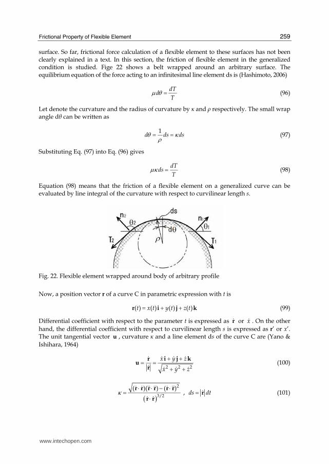
surface. So far, frictional force calculation of a flexible element to these surfaces has not been clearly explained in a text. In this section, the friction of flexible element in the generalized condition is studied. Fige 22 shows a belt wrapped around an arbitrary surface. The equilibrium equation of the force acting to an infinitesimal line element ds is (Hashimoto, 2006)

dT

dT

μ θ = (96)

Let denote the curvature and the radius of curvature by κ and ┩ respectively. The small wrap angle dθ can be written as

1

d ds dsθ κρ= = (97)


dT

dsT

μκ = (98)

Equation (98) means that the friction of a flexible element on a generalized curve can be evaluated by line integral of the curvature with respect to curvilinear length s.

Fig. 22. Flexible element wrapped around body of arbitrary profile

Now, a position vector r of a curve C in parametric expression with t is

( ) ( ) ( ) ( )t x t y t z t= + +r i j k (99)

Differential coefficient with respect to the parameter t is expressed as r$ or x$ . On the other

hand, the differential coefficient with respect to curvilinear length s is expressed as r’ or x’. The unit tangential vector u , curvature κ and a line element ds of the curve C are (Yano &

Ishihara, 1964)

2 2 2

x y z

x y z

+ += = + +i j kr

ur

$ $ $$$ $ $ $

(100)

( )2

3/2

( )( ) ( ), ds dtκ ⋅ ⋅ − ⋅= =⋅

r r r r r rr

r r

$ $ $$ $$ $ $$$

$ $ (101)

www.intechopen.com


260

For a plane curve of z=0 in Eq. (99), substituting Eq. (99) into Eq. (101) gives

2 22 2 3/2

,( )

xy xyds x y dt

x yκ −= = ++

$$$ $$$ $ $$ $

(102)

Substituting Eq. (102) into the left side of Eq. (98) gives

2 2

xy xyds dt

x yμκ μ −= +

$$$ $$$$ $

(103)

The unit principal normal vector m of the curve C is given by the formula (Yano & Ishihara, 1964)

'/ '

'

d dt

dt ds= =u u

m uu

(104)

Making use of Eq. (100) gives

{ }2 2 2

1' ( ) ( )

( )y xy xy x xy xy

x y= − + −+u i j$ $$$ $$$ $ $$$ $$$

$ $ (105)

2 22 2 2

'( )

xy xyx y

x yκ−= + =+u

$$$ $$$ $ $$ $

(106)


=2 2

y x

x y

− ++i j

m$ $

$ $ (107)

Here, the direction of the vector m is toward the center of curvature. Then, an outward

normal vector n can be defined as

=2 2

y x

x y

−= − +i j

n m$ $

$ $ (108)

The direction of the normal vector n is denoted by θ

1tanx

yθ − ⎛ ⎞−= ⎜ ⎟⎝ ⎠

$$

(109)

Differentiating Eq. (109) with respect to t gives

2 2

x y xy

x yθ −= +

$ $$ $$$$$ $

(110)

Comparing Eq. (110) with Eq. (103) gives

2 2

xy xyds dt dt

x yμκ μ μθ−= =+

$$$ $$$ $$ $

(111)

www.intechopen.com


261

Hence, making use of Eq. (111), integration of Eq. (98) becomes

( ) ( )2 1 2 1log /ds dt T Tμκ μθ μ θ θ= = − =∫ ∫ $ (112)

Equation (112) means that fraction of belt tension is determined by angular difference of the

outward normal vectors at the contact boundaries and is unrelated to the intermediate

profile. Equation (98) might be applied to the three dimensional problems.

As an example, let’s consider a rope spirally wrapped around a cylinder with radius a. The

parametric expression of a spiral with parameter t is (Yano & Ishihara, 1964)

cos , sin ,x a t y a t z bt= = = (113)

Substituting Eq. (113) into Eqs. (99) and (101) gives

( )2 2 2 2/ ,a a b ds a b dtκ = + = + (114)

Substituting Eq. (114) into Eq. (98) and integrating with respect to the parameter t from t1 to

t2 gives

( ) ( )22 1

21

1exp

1 /

Tt t

T b aμ⎧ ⎫⎪ ⎪= −⎨ ⎬⎪ ⎪+⎩ ⎭

(115)

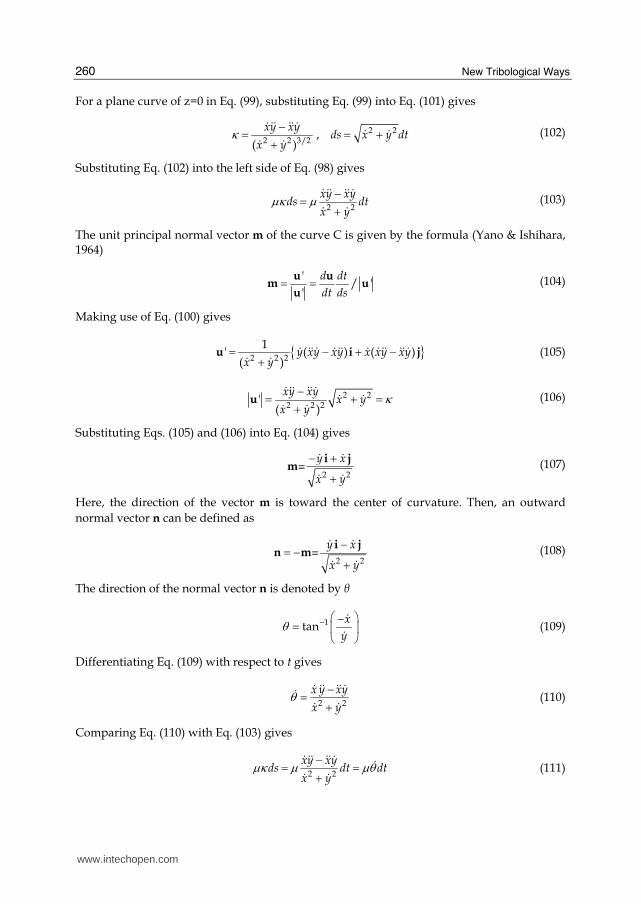
The member t2-t1 in Eq. (115) is usually a wrap angle for a plane problem. But it is not wrap angle in the three dimensional problem. In the case of b=0, Eq. (115) becomes well known Euler’s belt formula. On the other hand, when b becomes infinity, Eq. (115) yields T1=T2. Hence, for a three-dimensional problem, the frictional force of a rope is influenced on a way of wrapping. Figure 23 (a) shows some results of calculation of Eq. (115) provided t1=0 and t2=2n┨. Tension ratio T2/T1 decreases with an increment of the fraction of b/a. Let’s consider another example of a modified spiral defined by Eq. (116).

cos , sin , 14

tx a t y a t z bt

nπ⎛ ⎞= = = −⎜ ⎟⎝ ⎠ (116)

According to Eq. (116), it can be seen that the velocity component in z direction decreases linearly with parameter t and becomes 0 at t=2n┨. The components of Eq. (101) for the curve of Eq. (116) are

( )2 2 2

2 2 22 2

21 , ,

2 2 4

b t nt ba b a

n n n

ππ π π

−⎛ ⎞ ⎛ ⎞⋅ = + − ⋅ = + ⋅ =⎜ ⎟ ⎜ ⎟⎝ ⎠ ⎝ ⎠r r r r r r$ $ $$ $$ $ $$ (117)


( )2 2 2 2 2 2 2 2

2 23

2 22 2

4 1 4 4, 1

2

2 12

a a n b n n t t tds a b dt

nt

n a bn

π π πκ ππ π

+ + − + ⎛ ⎞= = + −⎜ ⎟⎝ ⎠⎧ ⎫⎪ ⎪⎛ ⎞+ −⎨ ⎬⎜ ⎟⎝ ⎠⎪ ⎪⎩ ⎭

(118)

www.intechopen.com


262

Fig. 23. Change of tension ratio T2/T1 with coefficient ratio b/a of spiral

Substituting Eq. (118) into Eq. (98) and integrating with respect to parameter t from t1=0 to t2=2n┨ gives

2 2 2

12

2 2 2 2 2 21

11log log tan

1 1

T

T

β γ βγμ βγ β γ γ γ β γ γ−⎧ ⎫⎛ ⎞ ⎛ ⎞⎛ ⎞ +⎪ ⎪⎜ ⎟ ⎜ ⎟= +⎨ ⎬⎜ ⎟ ⎜ ⎟ ⎜ ⎟⎝ ⎠ + + − + +⎪ ⎪⎝ ⎠ ⎝ ⎠⎩ ⎭

(119)

where ( )/ , 1 / 2b a nγ β π= =

Considering the case of ┛=0, namely b=0 of Eq. (119) requires limiting operation.

2 2

2 2 20

1lim log 2

1nγ

β γμ μ μ πβγ ββ γ γ γ→⎛ ⎞+⎜ ⎟ = =⎜ ⎟+ + −⎝ ⎠

(120)

Hence, the result of plane problem is included as a special case of ┛=0 in Eq. (119). Figure 23 (b) shows some results of calculation of Eq. (119). The tension ratio of T2/T1 in Fig. 23 (b) becomes larger than that of the corresponding value of Fig. 23 (a).

www.intechopen.com


263

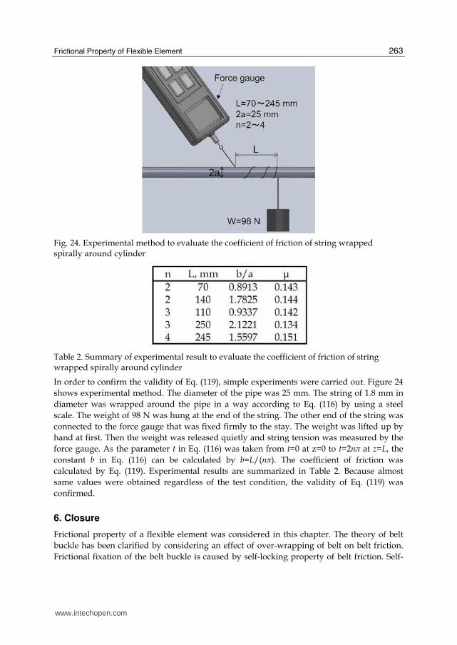
Fig. 24. Experimental method to evaluate the coefficient of friction of string wrapped spirally around cylinder

Table 2. Summary of experimental result to evaluate the coefficient of friction of string wrapped spirally around cylinder

In order to confirm the validity of Eq. (119), simple experiments were carried out. Figure 24

shows experimental method. The diameter of the pipe was 25 mm. The string of 1.8 mm in

diameter was wrapped around the pipe in a way according to Eq. (116) by using a steel

scale. The weight of 98 N was hung at the end of the string. The other end of the string was

connected to the force gauge that was fixed firmly to the stay. The weight was lifted up by

hand at first. Then the weight was released quietly and string tension was measured by the

force gauge. As the parameter t in Eq. (116) was taken from t=0 at z=0 to t=2n┨ at z=L, the

constant b in Eq. (116) can be calculated by b=L/(n┨). The coefficient of friction was

calculated by Eq. (119). Experimental results are summarized in Table 2. Because almost

same values were obtained regardless of the test condition, the validity of Eq. (119) was

confirmed.

6. Closure

Frictional property of a flexible element was considered in this chapter. The theory of belt

buckle has been clarified by considering an effect of over-wrapping of belt on belt friction.

Frictional fixation of the belt buckle is caused by self-locking property of belt friction. Self-

www.intechopen.com


264

locking occurs even in the case where a belt is wrapped around an axis two or more times.

Two conditions are required to bring about self-locking. One is smaller coefficient of belt-

belt friction than that of belt-axis friction. The other is larger wrap angle than the critical

wrap angle. Utilizing the self-locking property of belt, a novel one-way clutch was

developed. The problem of this clutch is how to get the smaller and stable coefficient of belt-

belt friction for long time use. Friction of a flexible element wrapped around a generalized

profile was studied. However, the friction of twisted flexible element in a thread, rope and

wire has not been clarified yet. Further research is required.

7. References

Hashimoto H., (2006). Tribology, Morikita publishing, ISBN 4-627-66591-1, Tokyo

Imado K., (2007). Study of Self-locking Mechanism of Belt Friction, Proceedings of the

STLE/ASME International Joint Tribology Conference, ISBN 0-7918-3811-0, San Diego

October 2007, ASME

Imado K., (2008 a). Study of Belt Buckle, Proceedings of the JAST Tribology Conference, pp.139-

140, ISSN 0919-6005, Tokyo, May 2008

Imado K., (2008 b). Study of Belt Friction in Over-Wrapped Condition, Tribology Online,

Vol.3, No.2, pp.76-79, ISSN 1881-2198

Imado K., Tominaga H., et al. (2010). Development of novel clutch utilizing self-locking

mechanisms of belt. Triloboy International, 43. pp.1127-1131, ISSN 0301-679X

J. A. Williams (1994). Engineering Tribology, Oxford University Press, ISBN 0-19-856503-8,

New York

Joseph F. Shelley (1990). Vector Mechanics for Engineers, McGraw-Hill, ISBN 0-07-056835-9,

New York

Yano K. & Ishihara S., (1964). Vector Analysis, Shokabo, 3341-01060-3067, Tokyo

www.intechopen.com

New Tribological WaysEdited by Dr. Taher Ghrib

ISBN 978-953-307-206-7Hard cover, 498 pagesPublisher InTechPublished online 26, April, 2011Published in print edition April, 2011

InTech EuropeUniversity Campus STeP Ri Slavka Krautzeka 83/A 51000 Rijeka, Croatia Phone: +385 (51) 770 447 Fax: +385 (51) 686 166www.intechopen.com

InTech ChinaUnit 405, Office Block, Hotel Equatorial Shanghai No.65, Yan An Road (West), Shanghai, 200040, China

Phone: +86-21-62489820 Fax: +86-21-62489821

This book aims to recapitulate old information's available and brings new information's that are with the fashionresearch on an atomic and nanometric scale in various fields by introducing several mathematical models tomeasure some parameters characterizing metals like the hydrodynamic elasticity coefficient, hardness,lubricant viscosity, viscosity coefficient, tensile strength .... It uses new measurement techniques verydeveloped and nondestructive. Its principal distinctions of the other books, that it brings practical manners tomodel and to optimize the cutting process using various parameters and different techniques, namely, usingwater of high-velocity stream, tool with different form and radius, the cutting temperature effect, that can bemeasured with sufficient accuracy not only at a research lab and also with a theoretical forecast. This bookaspire to minimize and eliminate the losses resulting from surfaces friction and wear which leads to a greatermachining efficiency and to a better execution, fewer breakdowns and a significant saving. A great part isdevoted to lubrication, of which the goal is to find the famous techniques using solid and liquid lubricant filmsapplied for giving super low friction coefficients and improving the lubricant properties on surfaces.

How to referenceIn order to correctly reference this scholarly work, feel free to copy and paste the following:

Keiji Imado (2011). Frictional Property of Flexible Element, New Tribological Ways, Dr. Taher Ghrib (Ed.),ISBN: 978-953-307-206-7, InTech, Available from: http://www.intechopen.com/books/new-tribological-ways/frictional-property-of-flexible-element

© 2011 The Author(s). Licensee IntechOpen. This chapter is distributedunder the terms of the Creative Commons Attribution-NonCommercial-ShareAlike-3.0 License, which permits use, distribution and reproduction fornon-commercial purposes, provided the original is properly cited andderivative works building on this content are distributed under the samelicense.

https://creativecommons.org/licenses/by-nc-sa/3.0/

frictional property of flexible element - intech -...

Documents