Ocean Sci., 14, 769–782, 2018https://doi.org/10.5194/os-14-769-2018© Author(s) 2018. This work is distributed underthe Creative Commons Attribution 4.0 License.

Frictional interactions between tidal constituentsin tide-dominated estuariesHuayang Cai1, Marco Toffolon2, Hubert H. G. Savenije3, Qingshu Yang1, and Erwan Garel41Institute of Estuarine and Coastal Research, School of Marine Sciences, Sun Yat-sen University, Guangzhou 510275, China2Department of Civil, Environmental and Mechanical Engineering, University of Trento, Trento, Italy3Department of Water Management, Faculty of Civil Engineering and Geosciences,Delft University of Technology, Delft, the Netherlands4Centre for Marine and Environmental Research (CIMA), University of Algarve, Faro, Portugal

Correspondence: Erwan Garel (egarel@ualg.pt)

Received: 18 April 2018 – Discussion started: 3 May 2018Revised: 23 July 2018 – Accepted: 27 July 2018 – Published: 8 August 2018

Abstract. When different tidal constituents propagate alongan estuary, they interact because of the presence of nonlinearterms in the hydrodynamic equations. In particular, due tothe quadratic velocity in the friction term, the effective fric-tion experienced by both the predominant and the minor tidalconstituents is enhanced. We explore the underlying mech-anism with a simple conceptual model by utilizing Cheby-shev polynomials, enabling the effect of the velocities ofthe tidal constituents to be summed in the friction term and,hence, the linearized hydrodynamic equations to be solvedanalytically in a closed form. An analytical model is adoptedfor each single tidal constituent with a correction factor toadjust the linearized friction term, accounting for the mu-tual interactions between the different tidal constituents bymeans of an iterative procedure. The proposed method is ap-plied to the Guadiana (southern Portugal–Spain border) andGuadalquivir (Spain) estuaries for different tidal constituents(M2, S2, N2, O1, K1) imposed independently at the estuarymouth. The analytical results appear to agree very well withthe observed tidal amplitudes and phases of the different tidalconstituents. The proposed method could be applicable toother alluvial estuaries with a small tidal amplitude-to-depthratio and negligible river discharge.

1 Introduction

Numerous studies have been conducted in recent decades tomodel tidal wave propagation along an estuary since an un-derstanding of tidal dynamics is essential for exploring theinfluence of human-induced (such as dredging for naviga-tional channels) or natural (such as global sea level rises)interventions on estuarine environments (Schuttelaars et al.,2013; Winterwerp et al., 2013). Analytical models are invalu-able tools and have been developed to study the basic physicsof tidal dynamics in estuaries; for instance, to examine thesensitivity of tidal properties (e.g., tidal damping or wavespeed) to change in terms of external forcing (e.g., spring–neap variations in amplitude) and geometry (e.g., depth orchannel length). However, most analytical solutions devel-oped to date, which make use of the linearized Saint-Venantequations, can only deal with one predominant tidal con-stituent (e.g., M2), which prevents consideration of the non-linear interactions between different tidal constituents. Theunderlying problem is that the friction term in the momen-tum equation follows a quadratic friction law, which causesnonlinear behavior, causing tidal asymmetry as the tide prop-agates upstream. If the friction law were linear, one wouldexpect that the effective frictional effect for different tidalconstituents (e.g., M2 and S2) could be computed indepen-dently (Pingree, 1983).

To explore the interaction between different constituentsof the tidal flow, the quadratic velocity u|u| (where u isthe velocity) is usually approximated by a truncated seriesexpansion, such as a Fourier expansion (Proudman, 1953;

Published by Copernicus Publications on behalf of the European Geosciences Union.

770 H. Cai et al.: Frictional interactions between tidal constituents

x

Planimetric view

Altimetric viewhA=Bh

ωt

Cross section

Tidal wave

η S torage areas

LWHW Bs

B

rs=Bs/B

Bs B

υz

u

h

z

Closed end

Figure 1. Geometry of a semi-closed estuary and basic notation (after Savenije et al., 2008). HW, high water; LW, low water.

Dronkers, 1964; Le Provost, 1973; Pingree, 1983; Fang,1987; Inoue and Garrett, 2007). If the tidal current is com-posed of one dominant constituent and a much smaller sec-ond constituent, it has been shown by many researchers (Jef-freys, 1970; Heaps, 1978; Prandle, 1997) that the weakerconstituent is acted on by up to 50 % more friction than actson the dominant constituent. However, this requires the as-sumption of a very small value of the ratio of the magni-tudes of the weaker and dominant constituents, which indi-cates that this is only a first-order estimation. Later, someresearchers extended the analysis to improve the accuracy ofestimates and to allow for more than two constituents (Pin-gree, 1983; Fang, 1987; Inoue and Garrett, 2007). Pingree(1983) investigated the interaction between M2 and S2 tides,resulting in a second-order correction of the effective frictioncoefficient acting on the predominant M2 tide and a fourth-order value for the weaker S2 constituent of the tide. Fang(1987) derived exact expressions of the coefficients of theFourier expansion of u|u| for two tidal constituents but didnot provide exact solutions for the case of three or more con-stituents. Later, Inoue and Garrett (2007) used a novel ap-proach to determine the Fourier coefficients of u|u|, whichallows the magnitude of the effective friction coefficient tobe determined for many tidal constituents. For the generaltwo-dimensional tidal wave propagation, the expansion ofquadratic bottom friction using a Fourier series was firstproposed by Le Provost (1973) and subsequently applied tospectral models for regional tidal currents (Le Provost et al.,1981; Le Provost and Fornerino, 1985; Molines et al., 1989).Building on the previous work by Le Provost (1973), the im-portance of quadratic bottom friction in tidal propagation anddamping was discussed by Kabbaj and Le Provost (1980)and reviews of friction terms in models were presented byLe Provost (1991).

In contrast, as noted by other researchers (Doodson, 1924;Dronkers, 1964; Godin, 1991, 1999), the quadratic veloc-ity u|u| is, mathematically, an odd function, and it is possibleto approximate it by using a two- or three-term expression,

such as αu+βu3 or αu+βu3+ ξu5, where α, β and ξ are

suitable numerical constants. The linear term αu representsthe linear superposition of different constituents, while thenonlinear interaction is attributed to a cubic term βu3 and afifth-order term ξu5. It is to be noted that such a method hasthe advantage of keeping the hydrodynamic equations solv-able in a closed form (Godin, 1991, 1999).

Previous studies explored the effect of frictional interac-tion between different tidal constituents by quantifying a fric-tion correction factor only (e.g., Dronkers, 1964; Le Provost,1973; Pingree, 1983; Fang, 1987; Godin, 1999; Inoue andGarrett, 2007). In this study, for the first time, the mutualinteractions between tidal constituents in the frictional termwere explored using a conceptual analytical model. Specifi-cally, a friction correction factor for each constituent was de-fined by expanding the quadratic velocity using a Chebyshevpolynomials approach. The model has subsequently been ap-plied to the Guadiana and Guadalquivir estuaries in southernIberia, for which cases the mutual interaction between thepredominantM2 tidal constituent and other tidal constituents(e.g., S2, N2, O1, K1) is explored.

2 Materials and methods

2.1 Hydrodynamic model

We are considering a semi-closed estuary that is forced byone predominant tidal constituent (e.g., M2) with the tidalfrequency ω = 2π/T , where T is the tidal period. As thetidal wave propagates into the estuary, it has a wave celerityof water level cA, a wave celerity of velocity cV, an ampli-tude of tidal elevation η, a tidal velocity amplitude υ, a phaseof water level φA, and a phase of velocity φV. The length ofthe estuary is indicated by Le.

The geometry of a semi-closed estuary is shown in Fig. 1,where x is the longitudinal coordinate, which is positive inthe landward direction, and z is the free surface elevation.The tidally averaged cross-sectional area A and width B are

Ocean Sci., 14, 769–782, 2018 www.ocean-sci.net/14/769/2018/

H. Cai et al.: Frictional interactions between tidal constituents 771

assumed to be exponentially convergent in the landward di-rection, as described by

A= A0 exp(−x/a), (1)

B = B0 exp(−x/b), (2)

where A0 and B0 are the respective values at the estuarymouth (where x = 0) and a and b are the convergence lengthsof cross-sectional area and width, respectively. We also as-sume a rectangular cross section, from which it follows thatthe tidally averaged depth is given by h= A/B. The possibleinfluence of storage area is described by the storage width ra-tio rS, defined as the ratio of the storage width BS (width ofthe channel at averaged high water level) to the tidally aver-aged width B (i.e., rS = BS/B).

With the above assumptions, the one-dimensional continu-ity equation reads

rS∂h

∂t+ u

∂h

∂x+h

∂u

∂x+hu

B

dBdx= 0, (3)

where t is the time and h the instantaneous depth. Assumingnegligible density effects, the one-dimensional momentumequations can be cast as follows

∂u

∂t+ u

∂u

∂x+ g

∂z

∂x+

gu|u|

K2h4/3 = 0, (4)

where g is the acceleration due to gravity and K is theManning–Strickler friction coefficient.

In order to obtain an analytical solution, we assume a neg-ligible river discharge and that the tidal amplitude is smallwith respect to the mean depth and follow Toffolon andSavenije (2011) to derive the linearized solution of the sys-tem of Eqs. (3) and (4). However, different from the stan-dard linear solutions, we will retain the mutual interactionamong different harmonics originating from the nonlinearfrictional term, which contains two sources of nonlinear-ity: the quadratic velocity u|u| and the variable depth in thedenominator. While we neglect the latter factor, consistentwith the assumption of small tidal amplitude, we will exploitChebyshev polynomials to represent the harmonic interac-tion in the quadratic velocity (see Sect. 3.1). For clarity, wereport here the linearized version of the momentum equation

∂u

∂t+ g

∂z

∂x+ κu|u| = 0 (5)

and the friction coefficient

κ =g

K2h4/3 . (6)

Toffolon and Savenije (2011) demonstrated that the tidalhydrodynamics in a semi-closed estuary are controlled bya few dimensionless parameters that depend on geometryand external forcing (for detailed information about analyt-ical solutions for tidal hydrodynamics, readers can refer to

Table 1. Definitions of dimensionless parameters.

Independent parameters Dependent parameters

Tidal amplitude at the mouth Tidal amplitudeζ0 = η0/h0 ζ = η/h

Friction number at the mouth Friction number

χ0 = rSc0ζ0g/(K2ωh0

4/3)

χ = rSc0ζg/(K2ωh

4/3)

Estuary shape Velocity numberγ = c0/(ωa) µ= υ/(rSζc0)= υh/(rSηc0)Estuary length Damping number for water levelL∗e = Le/L0 δA = c0dη/(ηωdx)

Damping number for velocityδV = c0dυ/(υωdx)Celerity number for water levelλA = c0/cACelerity number for velocityλV = c0/cVPhase differenceφ = φV−φA

Appendix A). They are defined in Table 1 and can be in-terpreted as follows: ζ0 is the dimensionless tidal amplitude(the subscript 0 indicating the seaward boundary condition);γ is the estuary shape number (representing the effect ofcross-sectional area convergence); χ0 is the friction num-ber (describing the role of the frictional dissipation); L∗e isthe dimensionless estuary length. The dimensional quantitiesused in the definition of the dimensionless parameters are asfollows: η0 is the tidal amplitude at the seaward boundary;

c0 =

√gh/rS is the frictionless wave celerity in a prismatic

channel; L0 = c0/ω is the tidal length scale related to thefrictionless tidal wave length by a factor 2π .

The main dependent dimensionless parameters are alsopresented in Table 1, including the following: ζ is the ac-tual tidal amplitude; χ is the actual friction number; µ is thevelocity number (the ratio of the actual velocity amplitude tothe frictionless value in a prismatic channel); λA and λV are,respectively, the celerity for elevation and velocity (the ratiobetween the frictionless wave celerity in a prismatic channeland actual wave celerity); δA and δV are, respectively, the am-plification number for elevation and velocity (describing therate of increase, δA (or δV) > 0, or decrease, δA (or δV) < 0,in the wave amplitudes along the estuary axis); φ = φV−φAis the phase difference between the phases of velocity andelevation.

It is important to remark that several nonlinear terms arepresent both in the continuity and in the momentum equa-tions (Parker, 1991), which are responsible, for instance, forthe internal generation of overtides (e.g.,M4). In this approx-imated approach, we disregard them and focus exclusively onthe mutual interaction among the external tidal constituentsmediated by the quadratic velocity dependence in the fric-tional term. In fact, the nonlinear quadratic velocity term cru-cially affects the propagation of the tidal waves associated

www.ocean-sci.net/14/769/2018/ Ocean Sci., 14, 769–782, 2018

772 H. Cai et al.: Frictional interactions between tidal constituents

with the different constituents that are already present in thetidal forcing at the estuary mouth.

2.2 Study areas

Both the Guadiana and Guadalquivir estuaries are located inthe southwest part of the Iberian Peninsula. These systemsare good candidates for the application of a 1-D hydrody-namic model of tidal propagation. Both estuaries feature asimple geometry, consisting of a single, narrow and moder-ately deep channel with relatively smooth bathymetric varia-tions. Moreover, their tidal prism exceeds their average fresh-water inputs by several orders of magnitude due to strongregulation by dams. Under these usual, low river dischargeconditions, both estuaries are well-mixed, and the water cir-culation is mainly driven by tides.

The Guadiana estuary, at the southern border betweenSpain and Portugal, connects the Guadiana River to the Gulfof Cádiz. Tidal water level oscillations are observed alongthe channel as far as a weir 78 km upstream of the rivermouth (Garel et al., 2009). Both the cross-sectional area andthe channel width are convergent and can be described by anexponential function, with convergence lengths of a = 31 kmand b = 38 km, respectively (Fig. 2). The flow depth is gen-erally between 4 and 8 m, with a mean depth of about 5.5 m(Garel, 2017). The tidal dynamics in the Guadiana estu-ary are derived from records obtained using eight pressuretransducers deployed for a period of 2 months (31 July to25 September 2015) approximately every 10 km along theestuary (from the mouth to ∼ 70 km upstream). The datawere collected during an extended (months-long) period ofdrought with negligible river discharge (always < 20 m3 s−1

over the preceding 5 months). For each station, the amplitudeand phase of elevation of the tidal constituents were obtainedfrom standard harmonic analysis of the observed pressurerecords using the “t-tide” Matlab toolbox (Pawlowicz et al.,2002). The harmonic results are displayed in Table 2. Nearthe mouth, the largest diurnal (K1), semidiurnal (M2) andquarter-diurnal (M4) frequencies are similar to those previ-ously reported at the same location based on pressure recordstaken over∼ 9 months (see Garel and Ferreira, 2013). In par-ticular, the value (ηK1 + ηO1)/(ηM2 + ηS2) is less than 0.1 atthe sea boundary, which indicates that the tide is dominantlysemidiurnal.

The Guadalquivir estuary is located in southern Spain, at∼ 100 km to the east of the Guadiana River mouth. The es-tuary has a length of 103 km starting from the mouth at San-lúcar de Barrameda to the Alcalá del Río dam. The geome-try of the Guadalquivir estuary can be approximated by ex-ponential functions with a convergence length of a = 60 kmfor the cross-sectional area and b = 66 km for the width (seeDiez-Minguito et al., 2012). The flow depth is more or lessconstant (7.1 m).

Tidal dynamics along the Guadalquivir estuary were an-alyzed by Diez-Minguito et al. (2012) based on harmonic

0 10 20 30 40 50 60 70 80Distance from the mouth x (km)

100

101

102

103

104

Dep

th (m

), w

idth

(m),

area

(m)2

Cross-sectional area

Depth

Width

Figure 2. Tidally averaged depth (m, black dots), width (m, bluedots) and cross-sectional area (m2, green dots) along the Guadianaestuary. Red lines represent exponential fit curves for the width andcross-sectional area.

analyses of field measurements collected from June to De-cember 2008. The amplitude and phase of tidal constituentsnear the mouth are highly similar to those at the entranceof the Guadiana estuary (Table 2), producing a semidiurnaland mesotidal signal with a mean spring tidal range of 3.5 m.In this paper, the tidal observations of the Guadalquivir es-tuary are taken directly from Diez-Minguito et al. (2012).The results apply to the low river discharge conditions (<40 m3 s−1) that usually predominate in the estuary.

3 Conceptual model

3.1 Representation of quadratic velocity u|u| using theChebyshev polynomials approach

Chebyshev polynomials can be used to approximate thequadratic dependence of the friction term on the velocity,u|u|. Adopting a two-term approximation, it is known that(Godin, 1991, 1999)

u|u| = υ̂2[α(uυ̂

)+β

(uυ̂

)3], (7)

where υ̂ is the sum of the amplitudes of all the harmonicconstituents. The Chebyshev coefficients α = 16/(15π) andβ = 32/(15π) were determined by the expansion of cos(nx)(n= 1, 2, . . . ) in powers of cos(x) (Godin, 1991, 1999). Itis important to note that, unlike series developments (e.g.,Fourier expansion), the Chebyshev coefficients α and β varywith the number of terms that are used in the development.Godin (1991) already showed that a two-term approximation(such as Eq. 7) is adequate to satisfactorily account for thefriction.

Ocean Sci., 14, 769–782, 2018 www.ocean-sci.net/14/769/2018/

H. Cai et al.: Frictional interactions between tidal constituents 773

Table 2. Tidal elevation amplitudes (m) and phases (◦) estimates (with 95 % confidence intervals in brackets) from harmonic analyses ofpressure records along the Guadiana estuary (x: distance from the mouth, km).

x (km) Msf O1 K1 N2 M2 S2 M4 M6

Amplitude (m)

2.4 0.01 (0.03) 0.06 (0.01) 0.07 (0.01) 0.23 (0.01) 0.97 (0.01) 0.37 (0.02) 0.02 (0.00) 0.01 (0.00)10.7 0.01 (0.07) 0.06 (0.01) 0.07 (0.01) 0.22 (0.01) 0.93 (0.01) 0.34 (0.01) 0.02 (0.01) 0.01 (0.00)22.8 0.03 (0.04) 0.06 (0.01) 0.07 (0.01) 0.20 (0.02) 0.86 (0.02) 0.29 (0.02) 0.04 (0.01) 0.02 (0.01)33.9 0.06 (0.05) 0.06 (0.01) 0.07 (0.01) 0.20 (0.02) 0.85 (0.02) 0.27 (0.02) 0.04 (0.01) 0.03 (0.01)43.6 0.06 (0.06) 0.06 (0.01) 0.07 (0.01) 0.21 (0.02) 0.87 (0.02) 0.27 (0.02) 0.05 (0.01) 0.03 (0.01)51.4 0.05 (0.05) 0.06 (0.01) 0.07 (0.01) 0.22 (0.02) 0.90 (0.02) 0.28 (0.02) 0.07 (0.01) 0.03 (0.01)60.1 0.07 (0.06) 0.06 (0.01) 0.07 (0.01) 0.22 (0.02) 0.93 (0.02) 0.30 (0.02) 0.08 (0.01) 0.04 (0.01)69.6 0.10 (0.06) 0.06 (0.01) 0.06 (0.01) 0.19 (0.03) 0.78 (0.03) 0.24 (0.03) 0.16 (0.03) 0.02 (0.01)

Phase (◦)

2.4 190 (149) 310 (6) 73 (5) 54 (4) 62 (1) 93 (2) 151 (8) 219 (18)10.7 8 (190) 319 (7) 85 (6) 68 (3) 75 (1) 108 (3) 103 (14) 237 (15)22.8 38 (66) 331 (9) 103 (7) 87 (4) 93 (1) 130 (3) 131 (12) 294 (16)33.9 49 (56) 343 (7) 116 (6) 104 (5) 109 (1) 151 (4) 166 (8) 336 (11)43.6 51 (58) 348 (8) 123 (8) 116 (5) 121 (1) 166 (4) 189 (6) 12 (14)51.4 48 (48) 352 (9) 128 (8) 123 (6) 128 (1) 175 (5) 203 (5) 43 (19)60.1 53 (58) 356 (9) 133 (8) 131 (6) 135 (1) 184 (5) 219 (4) 69 (21)69.6 51 (43) 7 (9) 146 (8) 146 (9) 148 (2) 200 (7) 261 (11) 15 (18)

For a single harmonic

u= υ1 cos(ω1t) , (8)

where υ1 is the velocity amplitude and ω1 its frequency,Eq. (7) can be expressed by exploiting standard trigonomet-ric relations as

u|u| ∼= υ21

[8

3πcos(ω1t)+

815π

cos(3ω1t)

]. (9)

Focusing only on the original harmonic constituent leads to

u|u| ∼=8

3πυ2

1 cos(ω1t) , (10)

which coincides exactly with Lorentz’s classical linearization(Lorentz, 1926) or a Fourier expansion of u|u| (Proudman,1953).

Considering a second tidal constituent, the velocity isgiven by

u= υ1 cos(ω1t)+ υ2 cos(ω2t)

= υ̂ [ε1 cos(ω1t)+ ε2 cos(ω2t)] , (11)

where υ2 and ω2 are the amplitude and frequency of the sec-ond constituent, and ε1 = υ1/υ̂ and ε2 = υ2/υ̂ are the ratiosof the amplitudes to that of the maximum possible velocityυ̂ = υ1+υ2. Note that the possible phase lag between the twoconstituents is neglected assuming a suitable time shift (In-oue and Garrett, 2007). In this case, the truncated Chebyshev

polynomials approximation of u|u| (focusing on two originaltidal constituents) is expressed as (see also Godin, 1999)

u|u| ∼=8

3πυ̂2 [F1ε1 cos(ω1t)+F2ε2 cos(ω2t)] , (12)

with

F1 =3π8

[α+β

(34ε2

1 +32ε2

2

)]=

15

(2+ 3ε2

1 + 6ε22

)=

15

(8+ 9ε2

1 − 12ε1

), (13)

F2 =3π8

[α+β

(34ε2

2 +32ε2

1

)]=

15

(2+ 3ε2

2 + 6ε21

)=

15

(5+ 9ε2

1 − 6ε1

), (14)

where F1 and F2 represent the effective friction coeffi-cients caused by the nonlinear interactions between tidal con-stituents. The last equality in Eqs. (13) and (14) is due to thefact that ε1+ ε2 = 1. It is worth noting that Eq. (12) is a rea-sonable approximation only if the amplitude of the secondaryconstituent is much smaller than that of the dominant one.

For illustration, approximations using Eqs. (7) and (12)for a typical tidal current with ε1 = 3/4 and ε2 = 1/4 aredisplayed in Fig. 3 for the case of two tidal constituents. Itcan be seen that the Chebyshev polynomials approximation(Eq. 7) matches the nonlinear quadratic velocity well, whileEq. (12), retaining only the original frequencies (ω1 and ω2),is still able to approximately capture the first-order trend ofthe quadratic term.

www.ocean-sci.net/14/769/2018/ Ocean Sci., 14, 769–782, 2018

774 H. Cai et al.: Frictional interactions between tidal constituents

0 1 2 3 4 5 6 7 8t (s) ×104

-0.4

-0.2

0

0.2

0.4

0.6

0.8

u|u|

u|u|Eq.(7)Eq.(12)

Figure 3. Approximation to the quadratic velocity u|u| by theChebyshev polynomials approach for the case of two tidal con-stituents (i.e., M2 and K1). Here, u= 0.6cos(ω1t)+ 0.2cos(ω2t),where ω1 and ω2 represent the tidal frequencies of M2 and K1, re-spectively.

It can be seen from Eqs. (13) and (14) that when ε2� 1(hence, ε1 ' 1 for the dominant tidal constituent), F1 ' 1,F2 ' 1.6; thus, the weaker constituent experiences propor-tionately 60 % more friction than the dominant constituent,which is slightly larger than the classical result of 50 % morefriction for the weaker tidal constituent. Figure 4 shows thesolutions of effective friction coefficients F1 and F2 as afunction of ε1 for the case of two constituents. As expected,we see a symmetric response of these coefficients in the func-tion of ε1 since ε1+ ε2 = 1. Specifically, we note that theeffective friction coefficient F1 reaches a minimum whenε1 = 2/3, when the velocity amplitude of the dominant con-stituent is twice as large as the weaker constituent.

Similarly, we are able to extend the same approach to thecase of a generic number n of astronomical tidal constituents(e.g., K1, O1, M2, S2, N2):

u=

n∑i=1

υ1 cos(ωi t)= υ̂n∑i=1

εi cos(ωi t) , (15)

in which the subscript i represents the ith tidal constituent.Considering only the original tidal constituents, the quadraticvelocity can be approximated as

u|u| ∼=8

3πυ̂2

n∑i=1

Fiεi cos(ωi t) , (16)

and the general expression for the effective friction coeffi-cients of j th tidal constituents is given by

Fj =3π8

{α+β

[n∑

i=1,i 6=j

32ε2i −

34ε2j

]}

0 0.1 0.2 0.3 0.4 0.5 0.6 0.7 0.8 0.9 10.8

1

1.2

1.4

1.6

F1

(a)

0 0.1 0.2 0.3 0.4 0.5 0.6 0.7 0.8 0.9 1ε1

0.8

1

1.2

1.4

1.6

F2

(b)

Figure 4. Computed effective friction coefficients F1 (a) and F2 (b)from Eqs. (13) and (14) as a function of ε1.

=15

(2+ 3ε2

j +

n∑i=1,i 6=j

6ε2i

). (17)

We provide the complete coefficients for the cases of one tothree constituents in Appendix B.

3.2 Effective friction in the momentum equation

For a single tidal constituent u= υ1 cos(ω1t), the quadraticvelocity term u|u| is often approximated by adoptingLorentz’s linearization equation (Eq. 10), and thus the fric-tion term in Eq. (5) becomes

κu|u| =

(κ

83πυ1

)u= ru, (18)

which is the “standard” case for a monochromatic wave,i.e., when we only deal with a predominant tidal constituent(e.g., M2).

For illustration of the method, we consider a tidal currentthat is composed of one dominant constituent (e.g., M2 withvelocity u1) and a weaker constituent (e.g., S2 with veloc-ity u2), which is a simple but important example in estuaries,i.e., u= u1+u2. In this case, the combination of Eq. (5) andthe Chebyshev polynomials expansion of u|u| (Eq. 12) yields

∂u1∂t+∂u2∂t+ g

∂z1∂x+ g

∂z2∂x+ κ

83πυ̂ (F1u1+F2u2)= 0, (19)

where z1 is the free surface elevation for the dominant con-stituent and z2 for the secondary constituent. Exploiting thelinearity of Eq. (19), we can solve the two problems indepen-dently. As a result, we see that the actual friction term that isfelt in Eq. (19) is different from that which would be felt bythe single constituent alone (Eq. 18).

Ocean Sci., 14, 769–782, 2018 www.ocean-sci.net/14/769/2018/

H. Cai et al.: Frictional interactions between tidal constituents 775

Introducing a general form of the linearized momentumequation for the generic ith constituent

∂ui

∂t+ g

∂zi

∂x+ firiui = 0, (20)

with

ri = κ8

3πυi, (21)

as in the standard case, we see that the effective friction termcontains a correction factor

fi =Fi

εi, (22)

through the coefficient Fi . Since the ratio εi can be quitesmall for a weaker constituent, the friction actually felt canbe significantly stronger.

4 Results

4.1 Hydrodynamic modeling incorporating the frictioncorrection factor

If there are many tidal constituents, then the friction experi-enced by one is affected by the others. As suggested by ourconceptual model, the mutual effects can be incorporated byusing the friction correction factor fn defined in Eq. (22) ifthe other (weaker) constituents are treated in the same wayas the predominant constituent. As a result, the friction num-ber χn for each tidal constituent can be modified as

χn = fnχ, (23)

where χ is the friction number (see definition in Table 1)experienced if only a single tidal constituent is considered.

We note that the modified friction number χn in Eq. (23)contains the friction coefficientK . In many applications,K iscalibrated separately for each tidal constituent to account forthe different friction exerted due to the combined tide, ei-ther changing K directly or through calibration of the differ-ent correction friction factors fn (see, e.g., Cai et al., 2015,2016). The current study aims at avoiding the need to ad-just K individually, so that only a single value of K needs tobe calibrated, based on the physical consideration that fric-tion mostly depends on bottom roughness, and the other fac-tors (tide interaction) are to be correctly modeled.

4.2 Procedure to study the propagation of the differentconstituents

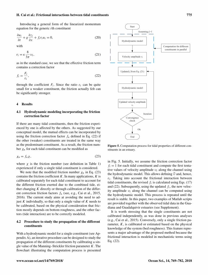
With a hydrodynamic model for a single constituent (see Ap-pendix A), an iterative procedure can be designed to study thepropagation of the different constituents by calibrating a sin-gle value of the Manning–Strickler friction parameterK . Theflowchart illustrating the computation process is presented

Start

Hydrodynamic model

Assuming fi=1

Velocity amplitude υi

Updated fi from Eq. (21)

Hydrodynamic model

Updated velocity amplitude υi

Convergencecheck

End

Ok

Iteration

Computation for different constituents in parallel

Figure 5. Computation process for tidal properties of different con-stituents in an estuary.

in Fig. 5. Initially, we assume the friction correction factorfi = 1 for each tidal constituent and compute the first tenta-tive values of velocity amplitude υi along the channel usingthe hydrodynamic model. This allows defining υ̂ and, hence,εi . Taking into account the frictional interaction betweentidal constituents, the revised fi is calculated using Eqs. (17)and (22). Subsequently, using the updated fi , the new veloc-ity amplitude υi along the channel can be computed usingthe hydrodynamic model. This process is repeated until theresult is stable. In this paper, two examples of Matlab scriptsare provided together with the observed tidal data in the Gua-diana and Guadalquivir estuaries (see Supplement).

It is worth stressing that the single constituents are notcalibrated independently, as was done in previous analyses(e.g., Cai et al., 2015). Conversely, only a single friction pa-rameter, K , is calibrated or estimated based on the physicalknowledge of the system (bed roughness). This feature repre-sents a major advantage of the proposed method because thefrictional interaction is modeled in mechanistic terms usingEq. (22).

www.ocean-sci.net/14/769/2018/ Ocean Sci., 14, 769–782, 2018

776 H. Cai et al.: Frictional interactions between tidal constituents

0 20 40 60 800.7

0.8

0.9

1

1.1

Am

plitu

de (m

) (a) M2

0

40

80

120

0 20 40 60 800.2

0.3

0.4

Am

plitu

de (m

)

(b) S2

0

40

80

120

Phas

e (°

)

0 20 40 60 800.1

0.2

0.3

Am

plitu

de (m

) (c) N2

0

40

80

120

0 20 40 60 80Distance from the mouth x (km)

0

0.1

0.2

Am

plitu

de (m

)

(d) K1

0

40

80

120

Phas

e (°

)

0 20 40 60 80Distance from the mouth x (km)

0

0.1

0.2

Am

plitu

de (m

) (e) O1

0

40

80

120

Phas

e (°

)

Analytical ηObserved ηAnalytical φAObserved φA

Figure 6. Tidal constituents (a)M2, (b) S2, (c) N2, (d)K1 and (e)O1, modeled against observed values of tidal amplitude (m) and phase (◦)of elevation along the Guadiana estuary.

4.3 Application to the Guadiana and Guadalquivirestuaries

In this study, the analytical model for a semi-closed estu-ary presented in Sect. 2.1 was applied to the Guadiana andGuadalquivir estuaries to reproduce the correct tidal behav-ior for different tidal constituents. The analytical results werecompared with observed tidal amplitude η and associatedphase of elevation φA.

The morphology of the Guadiana estuary was representedin the model with a constant depth (5.5 m), an exponentiallyconverging width (length scale, 38 km) and a constant stor-age ratio of 1 representative of the limited salt marsh areas(about 20 km2, see Garel, 2017). The Manning–Strickler fric-tion coefficient (K = 42 m1/3 s−1) was determined by cali-brating the model outputs (obtained using the iterative pro-cedure presented in Sect. 4.2) with observations. It can beseen from Fig. 6 that the computed tidal amplitude and phaseof elevation are in good agreement with the observed valuesfor different tidal constituents in the Guadiana estuary. TheN2 amplitude is slightly overestimated in the central part ofthe estuary, which may suggest that the harmonic analysishas some difficulties in resolving this constituent in relationto the length of the considered time series (54 days). In sup-port, the N2 amplitude (0.16 m) from a longer time series(85 days) collected in 2017 at 58 km from the mouth matchesthe model output better, while results for other constituentsare similar in 2015 and 2017 (Erwan Garel, personal com-munication, 2017). Otherwise, the correspondence is poorest

Table 3. Mean correction friction factor f for different tidal con-stituents along the Guadiana and Guadalquivir estuaries.

Tidal M2 S2 N2 K1 O1constituents

Guadiana 1.1 4.6 8.1 41.1 49.8Guadalquivir 1.1 5.4 9.7 40.7 43.7

for the semidiurnal constituents at the most upstream station,owing to the truncation of the lowest water levels by a silllocated about 65 km from the river mouth (Garel, 2017). Ta-ble 3 displays the mean friction correction coefficient f ob-tained from the iterative procedure to account for the non-linear interaction between different tidal constituents. In par-ticular, the mean friction correction factors f for the minorconstituents S2, N2, O1 and K1 are 4.6, 8.1, 41.1 and 49.8,respectively.

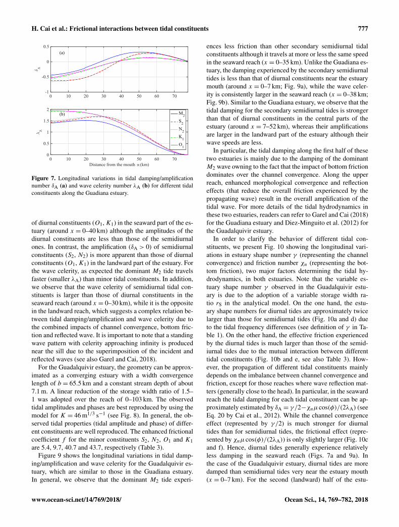
To understand the tidal dynamics between different tidalconstituents along the Guadiana estuary, the longitudinalvariations in the tidal damping/amplification number δA andcelerity number λA (see their definitions in Table 1) areshown in Fig. 7 where similar minor constituents in semid-iurnal (S2, N2) and diurnal (O1, K1) bands behave more orless the same. As shown in Fig. 7a, the minor constituents S2,N2, O1 and K1 experience more friction compared with thepredominant M2 tide. Interestingly, we observe a strongerdamping (δA < 0) of semidiurnal constituents (S2, N2) than

Ocean Sci., 14, 769–782, 2018 www.ocean-sci.net/14/769/2018/

H. Cai et al.: Frictional interactions between tidal constituents 777

0 10 20 30 40 50 60 70-1

-0.5

0

0.5

δA

(a)

0 10 20 30 40 50 60 70Distance from the mouth x (km)

0

0.5

1

1.5

2

λA

(b) M2S2N2K1O1

Figure 7. Longitudinal variations in tidal damping/amplificationnumber δA (a) and wave celerity number λA (b) for different tidalconstituents along the Guadiana estuary.

of diurnal constituents (O1,K1) in the seaward part of the es-tuary (around x = 0–40 km) although the amplitudes of thediurnal constituents are less than those of the semidiurnalones. In contrast, the amplification (δA > 0) of semidiurnalconstituents (S2, N2) is more apparent than those of diurnalconstituents (O1,K1) in the landward part of the estuary. Forthe wave celerity, as expected the dominant M2 tide travelsfaster (smaller λA) than minor tidal constituents. In addition,we observe that the wave celerity of semidiurnal tidal con-stituents is larger than those of diurnal constituents in theseaward reach (around x = 0–30 km), while it is the oppositein the landward reach, which suggests a complex relation be-tween tidal damping/amplification and wave celerity due tothe combined impacts of channel convergence, bottom fric-tion and reflected wave. It is important to note that a standingwave pattern with celerity approaching infinity is producednear the sill due to the superimposition of the incident andreflected waves (see also Garel and Cai, 2018).

For the Guadalquivir estuary, the geometry can be approx-imated as a converging estuary with a width convergencelength of b = 65.5 km and a constant stream depth of about7.1 m. A linear reduction of the storage width ratio of 1.5–1 was adopted over the reach of 0–103 km. The observedtidal amplitudes and phases are best reproduced by using themodel for K = 46 m1/3 s−1 (see Fig. 8). In general, the ob-served tidal properties (tidal amplitude and phase) of differ-ent constituents are well reproduced. The enhanced frictionalcoefficient f for the minor constituents S2, N2, O1 and K1are 5.4, 9.7, 40.7 and 43.7, respectively (Table 3).

Figure 9 shows the longitudinal variations in tidal damp-ing/amplification and wave celerity for the Guadalquivir es-tuary, which are similar to those in the Guadiana estuary.In general, we observe that the dominant M2 tide experi-

ences less friction than other secondary semidiurnal tidalconstituents although it travels at more or less the same speedin the seaward reach (x = 0–35 km). Unlike the Guadiana es-tuary, the damping experienced by the secondary semidiurnaltides is less than that of diurnal constituents near the estuarymouth (around x = 0–7 km; Fig. 9a), while the wave celer-ity is consistently larger in the seaward reach (x = 0–38 km;Fig. 9b). Similar to the Guadiana estuary, we observe that thetidal damping for the secondary semidiurnal tides is strongerthan that of diurnal constituents in the central parts of theestuary (around x = 7–52 km), whereas their amplificationsare larger in the landward part of the estuary although theirwave speeds are less.

In particular, the tidal damping along the first half of thesetwo estuaries is mainly due to the damping of the dominantM2 wave owning to the fact that the impact of bottom frictiondominates over the channel convergence. Along the upperreach, enhanced morphological convergence and reflectioneffects (that reduce the overall friction experienced by thepropagating wave) result in the overall amplification of thetidal wave. For more details of the tidal hydrodynamics inthese two estuaries, readers can refer to Garel and Cai (2018)for the Guadiana estuary and Diez-Minguito et al. (2012) forthe Guadalquivir estuary.

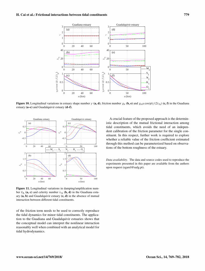
In order to clarify the behavior of different tidal con-stituents, we present Fig. 10 showing the longitudinal vari-ations in estuary shape number γ (representing the channelconvergence) and friction number χn (representing the bot-tom friction), two major factors determining the tidal hy-drodynamics, in both estuaries. Note that the variable es-tuary shape number γ observed in the Guadalquivir estu-ary is due to the adoption of a variable storage width ra-tio rS in the analytical model. On the one hand, the estu-ary shape numbers for diurnal tides are approximately twicelarger than those for semidiurnal tides (Fig. 10a and d) dueto the tidal frequency differences (see definition of γ in Ta-ble 1). On the other hand, the effective friction experiencedby the diurnal tides is much larger than those of the semid-iurnal tides due to the mutual interaction between differenttidal constituents (Fig. 10b and e, see also Table 3). How-ever, the propagation of different tidal constituents mainlydepends on the imbalance between channel convergence andfriction, except for those reaches where wave reflection mat-ters (generally close to the head). In particular, in the seawardreach the tidal damping for each tidal constituent can be ap-proximately estimated by δA = γ /2−χnµcos(φ)/(2λA) (seeEq. 20 by Cai et al., 2012). While the channel convergenceeffect (represented by γ /2) is much stronger for diurnaltides than for semidiurnal tides, the frictional effect (repre-sented by χnµcos(φ)/(2λA)) is only slightly larger (Fig. 10cand f). Hence, diurnal tides generally experience relativelyless damping in the seaward reach (Figs. 7a and 9a). Inthe case of the Guadalquivir estuary, diurnal tides are moredamped than semidiurnal tides very near the estuary mouth(x = 0–7 km). For the second (landward) half of the estu-

www.ocean-sci.net/14/769/2018/ Ocean Sci., 14, 769–782, 2018

778 H. Cai et al.: Frictional interactions between tidal constituents

0 50 1000.6

0.7

0.8

0.9

1

Am

plitu

de (m

) (a) M2

0

40

80

120

160

0 50 1000.1

0.2

0.3

0.4

Am

plitu

de (m

) (b) S2

0

40

80

120

160

Phas

e (°

)

0 50 1000

0.1

0.2

Am

plitu

de (m

)

(c) N2

0

40

80

120

160

0 50 100Distance from the mouth x (km)

0

0.1

0.2

Am

plitu

de (m

)

(d) K1

0

40

80

120

160

Phas

e (°

)

0 50 100Distance from the mouth x (km)

0

0.1

0.2

Am

plitu

de (m

) (e) O1

0

40

80

120

160

Phas

e (°

)

Analytical ηObserved ηAnalytical φAObserved φA

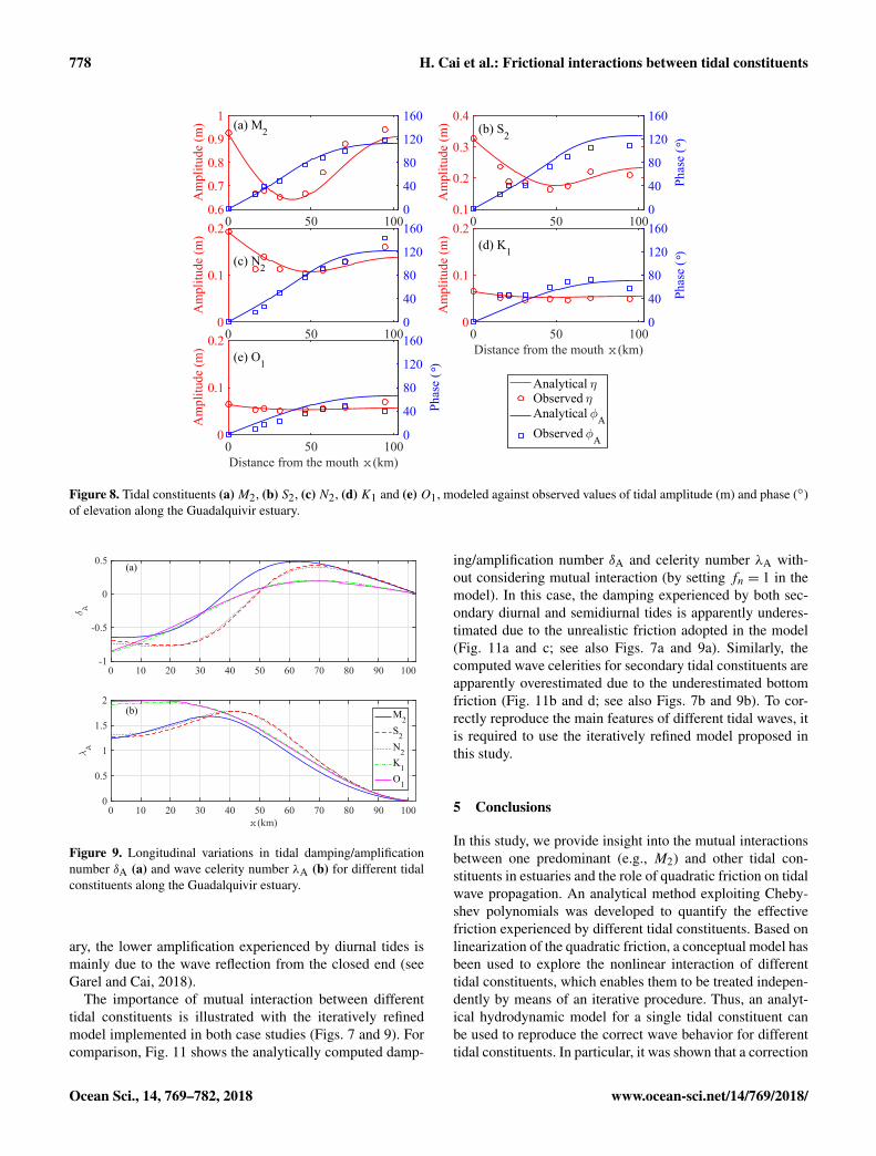
Figure 8. Tidal constituents (a)M2, (b) S2, (c) N2, (d)K1 and (e)O1, modeled against observed values of tidal amplitude (m) and phase (◦)of elevation along the Guadalquivir estuary.

0 10 20 30 40 50 60 70 80 90 100-1

-0.5

0

0.5

δA

(a)

0 10 20 30 40 50 60 70 80 90 100x (km)

0

0.5

1

1.5

2

λA

(b) M2S2N2K1O1

Figure 9. Longitudinal variations in tidal damping/amplificationnumber δA (a) and wave celerity number λA (b) for different tidalconstituents along the Guadalquivir estuary.

ary, the lower amplification experienced by diurnal tides ismainly due to the wave reflection from the closed end (seeGarel and Cai, 2018).

The importance of mutual interaction between differenttidal constituents is illustrated with the iteratively refinedmodel implemented in both case studies (Figs. 7 and 9). Forcomparison, Fig. 11 shows the analytically computed damp-

ing/amplification number δA and celerity number λA with-out considering mutual interaction (by setting fn = 1 in themodel). In this case, the damping experienced by both sec-ondary diurnal and semidiurnal tides is apparently underes-timated due to the unrealistic friction adopted in the model(Fig. 11a and c; see also Figs. 7a and 9a). Similarly, thecomputed wave celerities for secondary tidal constituents areapparently overestimated due to the underestimated bottomfriction (Fig. 11b and d; see also Figs. 7b and 9b). To cor-rectly reproduce the main features of different tidal waves, itis required to use the iteratively refined model proposed inthis study.

5 Conclusions

In this study, we provide insight into the mutual interactionsbetween one predominant (e.g., M2) and other tidal con-stituents in estuaries and the role of quadratic friction on tidalwave propagation. An analytical method exploiting Cheby-shev polynomials was developed to quantify the effectivefriction experienced by different tidal constituents. Based onlinearization of the quadratic friction, a conceptual model hasbeen used to explore the nonlinear interaction of differenttidal constituents, which enables them to be treated indepen-dently by means of an iterative procedure. Thus, an analyt-ical hydrodynamic model for a single tidal constituent canbe used to reproduce the correct wave behavior for differenttidal constituents. In particular, it was shown that a correction

Ocean Sci., 14, 769–782, 2018 www.ocean-sci.net/14/769/2018/

H. Cai et al.: Frictional interactions between tidal constituents 779

0 20 40 600

1

2

3

γ

Guadiana estuary

(a)

0 20 40 600

20

40

χn

(b)

0 20 40 60x (km)

0

0.5

1

χμ cos(φ)/(2λA)

(c)

0 50 1000

1

2

3

γ

Guadalquivir estuary

(d)

0 50 1000

20

40

χn

(e)

0 50 100x (km)

0

0.5

1(f)

M2

S2

N2

K1

O1

χμ cos(φ)/(2λA)

Figure 10. Longitudinal variations in estuary shape number γ (a, d), friction number χn (b, e) and χnµcos(φ)/(2λA) (c, f) in the Guadianaestuary (a–c) and Guadalquivir estuary (d–f).

0 20 40 60-1

-0.5

0

0.5

1

δA

Guadiana estuary

(a)

0 20 40 60x (km)

0

0.5

1

1.5

2

λA

(b)

0 50 100-1

-0.5

0

0.5

1

δA

Guadalquivir estuary

(c)

0 50 100x (km)

0

0.5

1

1.5

2

λA

(d)

M2 S2 N2 K1 O1

Figure 11. Longitudinal variations in damping/amplification num-ber δA (a, c) and celerity number λA (b, d) in the Guadiana estu-ary (a, b) and Guadalquivir estuary (c, d) in the absence of mutualinteraction between different tidal constituents.

of the friction term needs to be used to correctly reproducethe tidal dynamics for minor tidal constituents. The applica-tion to the Guadiana and Guadalquivir estuaries shows thatthe conceptual model can interpret the nonlinear interactionreasonably well when combined with an analytical model fortidal hydrodynamics.

A crucial feature of the proposed approach is the determin-istic description of the mutual frictional interaction amongtidal constituents, which avoids the need of an indepen-dent calibration of the friction parameter for the single con-stituent. In this respect, further work is required to explorewhether a reliable value of the friction coefficient estimatedthrough this method can be parameterized based on observa-tions of the bottom roughness of the estuary.

Data availability. The data and source codes used to reproduce theexperiments presented in this paper are available from the authorsupon request (egarel@ualg.pt).

www.ocean-sci.net/14/769/2018/ Ocean Sci., 14, 769–782, 2018

780 H. Cai et al.: Frictional interactions between tidal constituents

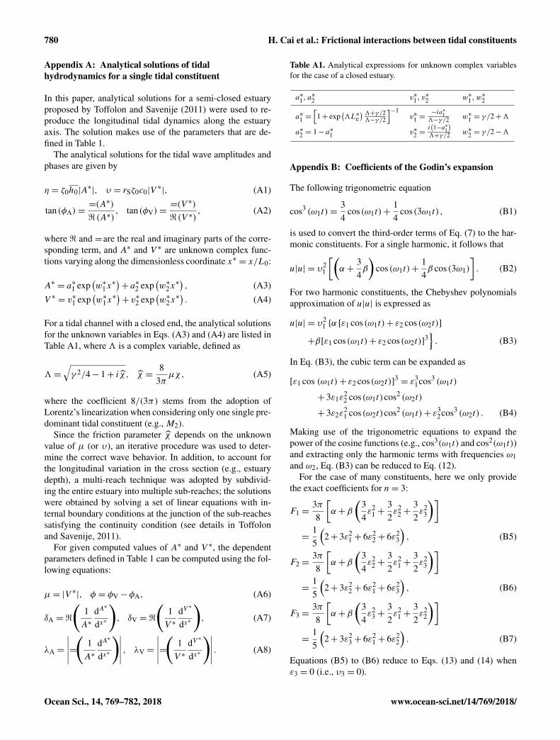
Appendix A: Analytical solutions of tidalhydrodynamics for a single tidal constituent

In this paper, analytical solutions for a semi-closed estuaryproposed by Toffolon and Savenije (2011) were used to re-produce the longitudinal tidal dynamics along the estuaryaxis. The solution makes use of the parameters that are de-fined in Table 1.

The analytical solutions for the tidal wave amplitudes andphases are given by

η = ζ0h0|A∗|, υ = rSζ0c0|V

∗|, (A1)

tan(φA)==(A∗)

<(A∗), tan(φV)=

=(V ∗)

<(V ∗), (A2)

where < and = are the real and imaginary parts of the corre-sponding term, and A∗ and V ∗ are unknown complex func-tions varying along the dimensionless coordinate x∗ = x/L0:

A∗ = a∗1 exp(w∗1x

∗)+ a∗2 exp

(w∗2x

∗), (A3)

V ∗ = v∗1 exp(w∗1x

∗)+ v∗2 exp

(w∗2x

∗). (A4)

For a tidal channel with a closed end, the analytical solutionsfor the unknown variables in Eqs. (A3) and (A4) are listed inTable A1, where 3 is a complex variable, defined as

3=

√γ 2/4− 1+ iχ̂ , χ̂ =

83πµχ, (A5)

where the coefficient 8/(3π) stems from the adoption ofLorentz’s linearization when considering only one single pre-dominant tidal constituent (e.g., M2).

Since the friction parameter χ̂ depends on the unknownvalue of µ (or υ), an iterative procedure was used to deter-mine the correct wave behavior. In addition, to account forthe longitudinal variation in the cross section (e.g., estuarydepth), a multi-reach technique was adopted by subdivid-ing the entire estuary into multiple sub-reaches; the solutionswere obtained by solving a set of linear equations with in-ternal boundary conditions at the junction of the sub-reachessatisfying the continuity condition (see details in Toffolonand Savenije, 2011).

For given computed values of A∗ and V ∗, the dependentparameters defined in Table 1 can be computed using the fol-lowing equations:

µ= |V ∗|, φ = φV−φA, (A6)

δA =<

(1A∗

dA∗

dx∗

), δV =<

(1V ∗

dV∗

dx∗

), (A7)

λA =

∣∣∣∣∣=(

1A∗

dA∗

dx∗

)∣∣∣∣∣ , λV =

∣∣∣∣∣=(

1V ∗

dV∗

dx∗

)∣∣∣∣∣ . (A8)

Table A1. Analytical expressions for unknown complex variablesfor the case of a closed estuary.

a∗1 , a∗2 v∗1 , v∗2 w∗1 , w∗2

a∗1 =[1+ exp

(3L∗e

) 3+γ /23−γ /2

]−1v∗1 =

−ia∗13−γ /2 w∗1 = γ /2+3

a∗2 = 1− a∗1 v∗2 =i(1−a∗1

)3+γ /2 w∗2 = γ /2−3

Appendix B: Coefficients of the Godin’s expansion

The following trigonometric equation

cos3 (ω1t)=34

cos(ω1t)+14

cos(3ω1t) , (B1)

is used to convert the third-order terms of Eq. (7) to the har-monic constituents. For a single harmonic, it follows that

u|u| = υ21

[(α+

34β

)cos(ω1t)+

14β cos(3ω1)

]. (B2)

For two harmonic constituents, the Chebyshev polynomialsapproximation of u|u| is expressed as

u|u| = υ21 {α [ε1 cos(ω1t)+ ε2 cos(ω2t)]

+β[ε1 cos(ω1t)+ ε2 cos(ω2t)]3}. (B3)

In Eq. (B3), the cubic term can be expanded as

[ε1 cos (ω1t)+ ε2 cos(ω2t)]3= ε3

1cos3 (ω1t)

+ 3ε1ε22 cos(ω1t)cos2 (ω2t)

+ 3ε2ε21 cos(ω2t)cos2 (ω1t)+ ε

32cos3 (ω2t) . (B4)

Making use of the trigonometric equations to expand thepower of the cosine functions (e.g., cos3(ω1t) and cos2(ω1t))and extracting only the harmonic terms with frequencies ω1and ω2, Eq. (B3) can be reduced to Eq. (12).

For the case of many constituents, here we only providethe exact coefficients for n= 3:

F1 =3π8

[α+β

(34ε2

1 +32ε2

2 +32ε2

3

)]=

15

(2+ 3ε2

1 + 6ε22 + 6ε2

3

), (B5)

F2 =3π8

[α+β

(34ε2

2 +32ε2

1 +32ε2

3

)]=

15

(2+ 3ε2

2 + 6ε21 + 6ε2

3

), (B6)

F3 =3π8

[α+β

(34ε2

3 +32ε2

1 +32ε2

2

)]=

15

(2+ 3ε2

3 + 6ε21 + 6ε2

2

). (B7)

Equations (B5) to (B6) reduce to Eqs. (13) and (14) whenε3 = 0 (i.e., υ3 = 0).

Ocean Sci., 14, 769–782, 2018 www.ocean-sci.net/14/769/2018/

H. Cai et al.: Frictional interactions between tidal constituents 781

The Supplement related to this article is available onlineat https://doi.org/10.5194/os-14-769-2018-supplement.

Author contributions. HC and EG conceived the study and wrotethe draft of the paper. MT, HHGS and QY contributed to the im-provement of the paper. All authors reviewed the paper.

Competing interests. The authors declare that they have no conflictof interest.

Acknowledgements. We acknowledge the financial support fromthe National Key R & D of China (grant no. 2016YFC0402600),from the National Natural Science Foundation of China (grantno. 51709287), from the Basic Research Program of Sun Yat-SenUniversity (grant no. 17lgzd12), and from the Water Resource Sci-ence and Technology Innovation Program of Guangdong Province(grant no. 2016-20). The work of Erwan Garel was supported byFCT research contract IF/00661/2014/CP1234.

Edited by: John M. HuthnanceReviewed by: David Bowers and Job Dronkers

References

Cai, H., Savenije, H. H. G., and Toffolon, M.: A new analyticalframework for assessing the effect of sea-level rise and dredgingon tidal damping in estuaries, J. Geophys. Res., 117, C09023,https://doi.org/10.1029/2012JC008000, 2012.

Cai, H., Toffolon, M., and Savenije, H. H. G.: Analytical investi-gation of superposition between predominant M2 and other tidalconstituents in estuaries, in: Proceedings of 36th IAHR WorldCongress, Delft – The Hague, 2015.

Cai, H., Toffolon, M., and Savenije, H. H. G.: An Analyt-ical Approach to Determining Resonance in Semi-ClosedConvergent Tidal Channels, Coast Eng. J., 58, 1650009,https://doi.org/10.1142/S0578563416500091, 2016.

Diez-Minguito, M., Baquerizo, A., Ortega-Sanchez, M., Navarro,G., and Losada, M. A.: Tide transformation in the Guadalquivirestuary (SW Spain) and process-based zonation, J. Geophys.Res., 117, C03019, https://doi.org/10.1029/2011jc007344, 2012.

Doodson, A. T.: Perturbations of Harmonic Tidal Constants, in:vol. 106 of 739, Proceedings of the Royal Society, London, 513–526, 1924.

Dronkers, J. J.: Tidal computations in River and Coastal Waters,Elsevier, New York, 1964.

Fang, G.: Nonlinear effects of tidal friction, Acta Oceanol. Sin., 6,105–122, 1987.

Garel, E.: Guadiana River estuary – Investigating the past, presentand future, in: Present Dynamics of the Guadiana Estuary, editedby: Moura, D., Gomes, A., Mendes, I., and Anibal, J., Universityof Algarve, Faro, Portugal, 15–37, 2017.

Garel, E. and Cai, H.: Effects of Tidal-Forcing Variations on TidalProperties Along a Narrow Convergent Estuary, Estuar. Coast,https://doi.org/10.1007/s12237-018-0410-y, in press, 2018.

Garel, E. and Ferreira, O.: Fortnightly changes in water transportdirection across the mouth of a narrow estuary, Estuar. Coast, 36,286–299, https://doi.org/10.1007/s12237-012-9566-z, 2013.

Garel, E., Pinto, L., Santos, A., and Ferreira, O.: Tidal and riverdischarge forcing upon water and sediment circulation at a rock-bound estuary (Guadiana estuary, Portugal), Estuar. Coast. ShelfS., 84, 269–281, https://doi.org/10.1016/j.ecss.2009.07.002,2009.

Godin, G.: Compact Approximations to the Bottom Friction Term,for the Study of Tides Propagating in Channels, Cont. Shelf Res.,11, 579–589, https://doi.org/10.1016/0278-4343(91)90013-V,1991.

Godin, G.: The propagation of tides up rivers with special consider-ations on the upper Saint Lawrence river, Estuar. Coast. Shelf S.,48, 307–324, https://doi.org/10.1006/ecss.1998.0422, 1999.

Heaps, N. S.: Linearized vertically-integrated equation for resid-ual circulation in coastal seas, Dtsch. Hydrogr. Z., 31, 147–169,https://doi.org/10.1007/BF02224467, 1978.

Inoue, R. and Garrett, C.: Fourier representation ofquadratic friction, J. Phys. Oceanogr., 37, 593–610,https://doi.org/10.1175/Jpo2999.1, 2007.

Jeffreys, H.: The Earth: Its Origin, History and Physical Consti-tution, 5th Edn., Cambridge University Press, Cambridge, UK,1970.

Kabbaj, A. and Le Provost, C.: Nonlinear tidal waves in channels: aperturbation method adapted to the importance of quadratic bot-tom friction, Tellus, 32, 143–163, https://doi.org/10.1111/j.2153-3490.1980.tb00942.x, 1980.

Le Provost, C.: Décomposition spectrale du terme quadratique defrottement dans les équations des marées littorales, C. R. Acad.Sci. Paris, 276, 653–656, 1973.

Le Provost, C.: Generation of Overtides and compound tides (re-view), in: Tidal Hydrodynamics, edited by: Parker, B., John Wi-ley and Sons, Hoboken, NJ, 269–295, 1991.

Le Provost, C. and Fornerino, M.: Tidal spectroscopy ofthe English Channel with a numerical model, J. Phys.Oceanogr., 15, 1009–1031, https://doi.org/10.1175/1520-0485(1985)015<1008:TSOTEC>2.0.CO;2, 1985.

Le Provost, C., Rougier, G., and Poncet, A.: Numer-ical modeling of the harmonic constituents of thetides, with application to the English Channel, J. Phys.Oceanogr., 11, 1123–1138, https://doi.org/10.1175/1520-0485(1981)011<1123:NMOTHC>2.0.CO;2, 1981.

Lorentz, H. A.: Verslag Staatscommissie Zuiderzee, Tech. rep., Al-gemene Landsdrukkerij, the Hague, the Netherlands, 1926.

Molines, J. M., Fornerino, M., and Le Provost, C.: Tidal spec-troscopy of a coastal area: observed and simulated tides ofthe Lake Maracaibo system, Cont. Shelf Res., 9, 301–323,https://doi.org/10.1016/0278-4343(89)90036-8, 1989.

Parker, B. B.: The relative importance of the various nonlinearmechanisms in a wide range of tidal interactions, in: Tidal Hy-drodynamics, edited by: Parker, B., John Wiley and Sons, Hobo-ken, NJ, 237–268, 1991.

Pawlowicz, R., Beardsley, B., and Lentz, S.: Classical tidalharmonic analysis including error estimates in MAT-

www.ocean-sci.net/14/769/2018/ Ocean Sci., 14, 769–782, 2018

782 H. Cai et al.: Frictional interactions between tidal constituents

LAB using T-TIDE, Comput. Geosci., 28, 929–937,https://doi.org/10.1016/S0098-3004(02)00013-4, 2002.

Pingree, R. D.: Spring Tides and Quadratic Friction, Deep-Sea Res. Pt. A, 30, 929–944, https://doi.org/10.1016/0198-0149(83)90049-3, 1983.

Prandle, D.: The influence of bed friction and vertical eddy vis-cosity on tidal propagation, Cont. Shelf Res., 17, 1367–1374,https://doi.org/10.1016/S0278-4343(97)00013-7, 1997.

Proudman, J.: Dynamical oceanography, Methuen, London, 1953.Savenije, H. H. G., Toffolon, M., Haas, J., and Veling,

E. J. M.: Analytical description of tidal dynamics inconvergent estuaries, J. Geophys. Res., 113, C10025,https://doi.org/10.1029/2007JC004408, 2008.

Schuttelaars, H. M., de Jonge, V. N., and Chernetsky, A.: Improvingthe predictive power when modelling physical effects of humaninterventions in estuarine systems, Ocean Coast. Manage., 79,70–82, https://doi.org/10.1016/j.ocecoaman.2012.05.009, 2013.

Toffolon, M. and Savenije, H. H. G.: Revisiting linearized one-dimensional tidal propagation, J. Geophys. Res., 116, C07007,https://doi.org/10.1029/2010JC006616, 2011.

Winterwerp, J. C., Wang, Z. B., van Braeckel, A., van Holland,G., and Kosters, F.: Man-induced regime shifts in small estuar-ies – II: a comparison of rivers, Ocean Dynam., 63, 1293–1306,https://doi.org/10.1007/s10236-013-0663-8, 2013.

Ocean Sci., 14, 769–782, 2018 www.ocean-sci.net/14/769/2018/