frictional contact of an anisotropic piezoelectric plate … · frictional contact of an...
TRANSCRIPT
Pre-Publicacoes do Departamento de MatematicaUniversidade de CoimbraPreprint Number 07–16
FRICTIONAL CONTACT OF AN ANISOTROPICPIEZOELECTRIC PLATE
ISABEL N. FIGUEIREDO AND GEORG STADLER
Abstract: The purpose of this paper is to derive and study a new asymptoticmodel for the equilibrium state of a thin anisotropic piezoelectric plate in frictionalcontact with a rigid obstacle. In the asymptotic process, the thickness of the piezo-electric plate is driven to zero and the convergence of the unknowns is studied.This leads to two-dimensional Kirchhoff-Love plate equations, in which mechanicaldisplacement and electric potential are partly decoupled. Based on this model nu-merical examples are presented that illustrate the mutual interaction between themechanical displacement and the electric potential. We observe that, compared topurely elastic materials, piezoelectric bodies yield a significantly different contactbehavior.
Keywords: contact, friction, asymptotic analysis, anisotropic material, piezoelec-tricity, plate.
AMS Subject Classification (2000): 74K20, 78M35, 74M15, 74M10, 74F15.
1. Introduction
The generation of electric charges in certain crystals when subjected tomechanical force was discovered in 1880 by Pierre et Jacques Curie and isnowadays known as piezoelectric effect (or direct piezoelectric effect). Theinverse phenomenon, that is, the generation of mechanical stress and strain incrystals when subjected to electric fields is called inverse piezoelectric effectand was predicted in 1881 by Lippmann (see [17]). Piezoelectric materialsare solids exhibiting this kind of interaction between mechanical and elec-tric properties. This provides them with sensor (direct effect) and actuator(inverse effect) capabilities making them extremely useful in a wide range ofpractical applications in aerospace, mechanical, electrical, civil and biomedi-cal engineering (see [29]). In many of these applications, additionally contactphenomena can occur or may be used on purpose, e.g., for measurement de-vices.
Received April 15, 2007.This work is partially supported by the project ”Mathematical Analysis of Piezoelectric Prob-
lems” (POCTI/MAT/59502/2004, Fundacao para a Ciencia e a Tecnologia, Portugal).
1
2 I. N. FIGUEIREDO AND G. STADLER
The aim of this paper is to derive, mathematically justify and numericallystudy a new bi-dimensional model for the equilibrium state of an anisotropicpiezoelectric thin plate possibly in frictional contact with a rigid foundation.The derivation of the reduced (or lower-dimensional) model is done usingan asymptotic procedure. It will turn out that the resulting equations aredefined in the middle plane of the plate.
Let us start with motivating our interest in this problem. It was observedthat, if no contact and friction conditions have to be taken into account,for certain problems the mechanical and the electric parts of the equationsdecouple in an asymptotic process [11, 8, 28, 26] (see [1, 7, 23, 25, 33] forrelated results where only partial or no decoupling occurs). In the presenceof contact and friction it is not at all obvious if similar results hold true.We are also interested in numerically studying the behavior of piezoelectricmaterials, and by these means gain a better understanding for their propertiesand features.
Asymptotic methods have been widely used to deduce reduced models forplates, shells or rods. For the main ideas and bibliographic references see [3, 4,5] for elastic plates, [6] for shells, and [32] for rods. For thin plates, asymptoticanalysis applies to the thickness variable and can be briefly summarized asfollows: Starting with the variational three-dimensional equations for a platewith thickness h, these equations are scaled to a domain independent ofh. Assuming appropriate scalings for the data and unknowns, one thenlets h → 0 and studies the convergence of the unknowns as well as theproperties of the limit variables. Rescaling to the original domain then resultsin reduced model equations. For a general theory of asymptotic expansionsfor variational problems that depend on a small parameter we refer to [21].
We consider, in this paper, an anisotropic piezoelectric plate whose me-chanical displacements are restricted due to possible contact with a rigidinsulated foundation. The contact is unilateral (i.e., the contact region isnot known in advance) and is modelled by the classical Signorini conditions.For the frictional behavior of the plate, the Tresca friction law is used. Thevariational formulation of this plate problem is a variational inequality of thesecond kind, see [9, 18]. The unknowns are the mechanical displacement andthe electric potential. The original, three-dimensional plate is subject to con-tact and friction on a part of its surface. While in the asymptotic procedure
FRICTIONAL CONTACT OF AN ANISOTROPIC PIEZOELECTRIC PLATE 3
the system equations become two-dimensional, the contact and friction con-ditions remain similar to contact conditions occurring in three-dimensionalelasticity.
Note that for modeling friction in physical applications, often the Coulombrather than the Tresca friction law is used (see [9]). Since for the numericalrealization of Coulomb friction usually a sequence of Tresca friction problemsis used, Tresca friction is not only of theoretical but also practical relevance.Such as sequence of Tresca problems is also solved in our numerical study todiscuss a problem with Coulomb friction.
In the literature, several authors deal with asymptotic models for piezoelec-tric structures. We mention [26] for piezoelectric plates including magneticeffects, [28] for piezoelectric thin plates with homogeneous isotropic elasticitycoefficients, [23, 25, 33, 11, 12] for anisotropic piezoelectric plates and rods,[7] for geometrically nonlinear thin piezoelectric shells, and [27] for the mod-elling of eigenvalue problems for thin piezoelectric shells. However, thesepapers do not take into account the effects of possible contact or frictionwith a rigid foundation; nevertheless for elastic rods and shells, one findsasymptotic frictionless contact models in [32] and [20], respectively. On theother hand, there are papers dealing with contact and friction of piezoelectricmaterials that do not use an asymptotic procedure to reduce the model; werefer to [22], where two different variational formulations for the modellingof unilateral frictionless contact are established as well as [2] for primal anddual formulations of frictional contact problems. In [30, 31], mathematicalanalysis of frictional contact problems with piezoelectric materials can befound; for error estimates and numerical simulations we refer to [15]. In allof the above references either none or only few numerical simulations can befound.
The main contributions of this paper are twofold: Firstly, the application ofthe asymptotic method to the variational inequality of the second kind thatdescribes the anisotropic piezoelectric plate. Due to the presence of frictionand contact conditions, the convergence proof in the asymptotic procedure issignificantly more involved than in the unconstrained case (see [11, 28]). Oursecond main contribution is the numerical study of the limit problem takinginto account contact and friction. These conditions are similar to three-dimensional elasticity contact problems, where their numerical treatment isknown to be a challenging task.
4 I. N. FIGUEIREDO AND G. STADLER
We finish this introduction with a sketch of the structure of this paper. Inthe next section, the three-dimensional plate model is described. In Section3, we apply the asymptotic analysis and prove strong convergence of the un-knowns. Finally, in Section 4 we report on numerical tests for the asymptoticequations.
2. The 3D plate problem
Notations and geometry. Let ω ⊂ IR2 be a bounded domain with
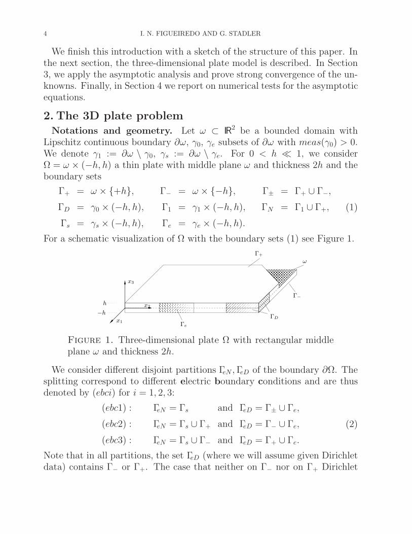
Lipschitz continuous boundary ∂ω, γ0, γe subsets of ∂ω with meas(γ0) > 0.We denote γ1 := ∂ω \ γ0, γs := ∂ω \ γe. For 0 < h ≪ 1, we considerΩ = ω × (−h, h) a thin plate with middle plane ω and thickness 2h and theboundary sets
Γ+ = ω × +h, Γ− = ω × −h, Γ± = Γ+ ∪ Γ−,
ΓD = γ0 × (−h, h), Γ1 = γ1 × (−h, h), ΓN = Γ1 ∪ Γ+,
Γs = γs × (−h, h), Γe = γe × (−h, h).(1)
For a schematic visualization of Ω with the boundary sets (1) see Figure 1.
Γe
x1
x3
x2
Γ−
Γ+
ω
ΓD
−h
h
Figure 1. Three-dimensional plate Ω with rectangular middleplane ω and thickness 2h.
We consider different disjoint partitions ΓeN ,ΓeD of the boundary ∂Ω. Thesplitting correspond to different electric boundary conditions and are thusdenoted by (ebci) for i = 1, 2, 3:
(ebc1) : ΓeN = Γs and ΓeD = Γ± ∪ Γe,
(ebc2) : ΓeN = Γs ∪ Γ+ and ΓeD = Γ− ∪ Γe,
(ebc3) : ΓeN = Γs ∪ Γ− and ΓeD = Γ+ ∪ Γe.
(2)
Note that in all partitions, the set ΓeD (where we will assume given Dirichletdata) contains Γ− or Γ+. The case that neither on Γ− nor on Γ+ Dirichlet

FRICTIONAL CONTACT OF AN ANISOTROPIC PIEZOELECTRIC PLATE 5
data for the electric potential are given requires a slightly different treatmentthan the one chosen in this paper, see Remark 1 on page 23.
Points of Ω are denoted by x = (x1, x2, x3), where the first two components(x1, x2) ∈ ω are independent of h and x3 ∈ (−h, h). We denote by n =(n1, n2, n3) the unit outward normal vector to ∂Ω. Throughout the paper,the Latin indices i, j, k, l, . . . are taken from 1, 2, 3, while the Greek indicesα, β, . . . from 1, 2. The summation convention with respect to repeatedindices is employed, that is, aibi =
∑3i=1 aibi. Moreover we denote by a · b =
aibi the inner product of the vectors a = (ai) and b = (bi), by Ce = (Cijklekl)the contraction of a fourth order tensor C = (Cijkl) with a second ordertensor e = (ekl) and by Ce : d = Cijklekldij the inner product of the tensorsCe and d = (dij). Given a function θ(x) defined in Ω we denote by ∂iθ = ∂θ
∂xi
its partial derivative with respect to xi.In the sequel, for an open subset Υ ⊂ IR
n, n = 2, 3, we define D(Υ) to bethe space of infinitely often differentiable functions with compact support onΥ. We denote by D′(Υ) the dual space of D(Υ), often called the space ofdistributions on Υ. For m = 1, 2, the Sobolev spaces Hm(Υ) are defined by
H1(Υ) =
v ∈ L2(Υ) : ∂iv ∈ L2(Υ) for i = 1, . . . , n
,
H2(Υ) =
v ∈ L2(Υ) : ∂iv, ∂ijv ∈ L2(Υ) for i, j = 1, . . . , n
,
where L2(Υ) = v : Υ → IR,∫
Υ |v|2dΥ < ∞ and the partial derivativesare interpreted as distributional derivatives. Moreover, for v ∈ (H1(Ω))3
we denote by vn := v · n and vt := v − vnn the normal and tangentialcomponents of v on the boundary of Ω, respectively. Similarly, for a secondorder symmetric tensor field τ = (τij) ∈ (L2(Ω))9 we denote its normaland tangential components on the boundary of Ω as τn := (τn) · n andτt := (τn)−τnn, respectively. Using the summation convention, this becomesτn := τijninj and τt = (τti) where τti := τijnj − τnni. In addition, we denoteby | · | the Euclidean norm in IR
3.3D plate in frictional contact – classical formulation. We consider
a piezoelectric anisotropic plate which in its reference configuration occupiesthe domain Ω. It is held fixed on ΓD and submitted to a mechanical volumeforce of density f in Ω and a mechanical surface traction of density g on ΓN .On its lower face Γ− it may be in frictional contact with the rigid foundation(which is assumed to be an insulator). We denote by s : Γ− −→ IR
+ theinitial gap between the rigid foundation and the boundary Γ− measured in the

6 I. N. FIGUEIREDO AND G. STADLER
direction of the outward unit normal vector n. To model the frictional contactwe use the classical Signorini contact conditions and the Tresca friction law(see [9]).
We assume that the plate is subject to an electric volume charge of densityr. Moreover, we suppose given an electric surface charge of density θ on ΓeN
and an electric potential equal to ϕ0 applied to ΓeD, where the pair ΓeN ,ΓeD
is defined as in one of the cases (ebci), i = 1, 2, 3 above. Note that the lowersubscripts eN and eD in ΓeN and ΓeD refer to electric (e) Neumann (N) andDirichlet (D) boundary conditions, respectively, while the lower subscripts N
and D in ΓN and ΓD refer to mechanical (Neumann and Dirichlet) boundaryconditions.
We now give the classical (i.e., strong) equations defining the mechanicaland electric equilibrium state of the plate Ω. The equilibrium is describedby the following five groups of equations and boundary conditions, whoseunknowns are the mechanical displacement vector u : Ω → IR
3 and the(scalar) electric potential ϕ : Ω → IR.
Mechanical equilibrium equations and boundary conditions
−divσ(u, ϕ) = f (i.e., − ∂jσij(u, ϕ) = fi) in Ω,
σ(u, ϕ)n = g (i.e., σij(u, ϕ)nj = gi) on ΓN ,
u = 0 on ΓD.
(3a)
Maxwell-Gauss equations and electric boundary conditions (ebci), i = 1, 2, 3
divD(u, ϕ) = r (i.e., ∂iDi(u, ϕ) = r) in Ω,
D(u, ϕ)n = θ (i.e., Di(u, ϕ)ni = θ) on ΓeN ,
ϕ = ϕ0 on ΓeD.
(3b)
Constitutive equations[
σij(u, ϕ) = Cijklekl(u) − PkijEk(ϕ) in Ω,
Dk(u, ϕ) = Pkijeij(u) + εklEl(ϕ) in Ω.(3c)
Signorini’s contact conditions
un ≤ s, σn ≤ 0, σn(un − s) = 0 on Γ−. (3d)
FRICTIONAL CONTACT OF AN ANISOTROPIC PIEZOELECTRIC PLATE 7
Tresca’s law of friction
|σt| ≤ q, and
|σt| < q ⇒ ut = 0,
|σt| = q ⇒ ∃c ≥ 0 : ut = −cσt
on Γ−. (3e)
The mechanical equilibrium equations (3a) express the balance of mechanicalloads and internal stresses. The electric displacement field D is governedby the Maxwell-Gauss equations (3b), and the constitutive equations (3c)characterize piezoelectricity. They define the interaction between the stresstensor σ : Ω → IR
9, the electric displacement vector D : Ω → IR3, the linear
strain tensor e(u) and the electric field vector E(ϕ), the latter two tensorsgiven by
e(u) = 12
(
∇u+ (∇u)⊤)
(i.e., eij(u) = 12
(
∂iuj + ∂jui))
E(ϕ) = −∇ϕ (i.e., Ei(ϕ) = −∂iϕ).
In (3c), C = (Cijkl) is the elastic fourth order, P = (Pijk) the piezoelectricthird order and ε = (εij) is the dielectric second order tensor field. TheSignorini law (3d) describes the contact and frictional behavior of the platewith a rigid foundation. If the plate is not in contact with the rigid foundation(i.e., un < s), the normal stress vanishes, i.e., σn = 0. For un = s, thatis, the plate is in contact with the obstacle, the normal stress componentσn is nonpositive. These conditions are the complementarity conditions forcontact. Finally, the conditions (3e) model the frictional behavior of theplate, where q ≥ 0 is a function representing the prescribed friction bound.Briefly, (3e) expresses the fact that on the contact boundary Γ− the Euclideannorm of the tangential stress component cannot exceed the given frictionbound q, that slip occurs if this norm equals q, and stick if it is smaller thanq. Moreover, slip can only occur in the negative direction of σt. Note thatthe regions where contact and slip or stick occur are not known a priori.This makes contact problems with friction free boundary problems, whichare theoretically and practically challenging.
We assume the following hypotheses on the data
f ∈(
L2(Ω))3, g ∈
(
L2(ΓN))3, r ∈ L2(Ω), θ ∈ L2(ΓeN),
ϕ0 ∈ H1/2(ΓeD), s ∈ H1/2(Γ−), q ∈ L2(Γ−).
8 I. N. FIGUEIREDO AND G. STADLER
Moreover, the tensor fields C = (Cijkl), P = (Pijk) and ε = (εij) are definedon ω × [−1, 1] for x = (x1, x2,
x3
h ). Defining them on the reference plateω × [−1, 1] makes them independent of h in the transformed variables alsoused in the next section. The tensors Cijkl, Pijk, εij are assumed to besufficiently smooth functions that satisfy the following symmetries Cijkl =Cjikl = Cklij, Pijk = Pikj, εij = εji. Moreover, C and ε are assumed to becoercive, that is there exist c1, c2 > 0 such that
Cijkl(x)MklMij ≥ c1
3∑
i,j=1
(Mij)2 and εij(x)θiθj ≥ c2
3∑
i=1
θ2i
for every symmetric 3 × 3 real valued matrix M , every vector θ ∈ IR3 and
every x ∈ ω × [−1, 1].3D-plate in frictional contact – weak formulation. We now give
the weak or variational formulation of (3a)-(3e). We define the space ofadmissible mechanical displacements
V :=
v ∈(
H1(Ω))3
: v|ΓD= 0
that we endow with the norm ‖v‖V = ‖∇v‖(L2(Ω))9, which, due to the Poincareinequality is equivalent to the usual H1-norm. Moreover, we introduce theconvex cone
K :=
v ∈ V : vn ≤ s on Γ−
, where vn = −v3,
as well as the space of admissible electric potentials
Ψ :=
ψ ∈ H1(Ω) : ψ|ΓeD= 0
,
in which we use the norm ‖ψ‖Ψ = ‖∇ψ‖(L2(Ω))3 (which is also equivalent tothe usual H1-norm).
Next, we briefly sketch how the variational formulation of (3a)-(3e) is ob-tained. Using the Green formula in (3a), we obtain for any v ∈ K
∫
Ω
σij eij(v − u) dx−∫
∂Ω
σij nj (vi − ui) dΓN =
∫
Ω
fi(vi − ui) dx. (4)
Since v = u = 0 on ΓD, σij nj = gi on ΓN , ∂Ω = ΓD ∪ ΓN ∪ Γ− and due to
σij nj (vi − ui) = σt (vt − ut) + σn (vn − un)
= σt (vt − ut) + σn (vn − s) − σn (un − s),
FRICTIONAL CONTACT OF AN ANISOTROPIC PIEZOELECTRIC PLATE 9
(4) becomes, using σn(vn − s) ≥ 0 and σn(un − s) = 0 on Γ−,∫
Ω
σij eij(v−u) dx−∫
Ω
fi(vi−ui) dx−∫
ΓN
gi(vi−ui) dΓN ≥∫
Γ−
σt (vt−ut) dx.
(5)Adding j(v) − j(u) to both sides of (5), where
j(v) :=
∫
Γ−
q |vt| dΓ−, with vt = v − vnn = (v1, v2, 0),
and using∫
Ω
(
σt (vt − ut) + q|vt| − q|ut|)
dx ≥ 0,
we obtain∫
Ω
σij eij(v−u) dx+j(v)−j(u)−∫
Ω
fi(vi−ui) dx−∫
ΓN
gi(vi−ui) dΓN ≥ 0. (6)
Next, from (3b) we have for any ψ ∈ Ψ
−∫
Ω
Di ∂iψ dx+
∫
ΓeN
θ ψ dΓeN =
∫
Ω
r ψ dx, (7)
where Di ni = θ on ΓeN and ψ = 0 on ΓeD have been used. Summing (6) and(7), using the constitutive equations (3c) and the transformation ϕ = ϕ+ϕ0,we obtain as weak formulation of (3a)-(3e) the following elliptic variationalinequality of the second kind [13, 14]
Find (u, ϕ) ∈ K × Ψ such that:
b(
(u, ϕ), (v − u, ψ))
+ j(v) − j(u) ≥ l(
(v − u, ψ))
∀(v, ψ) ∈ K × Ψ,
(8)where
b(
(u, ϕ), (v, ψ))
:=∫
ΩCe(u) : e(v) dx+∫
Ω εij ∂iϕ ∂jψ dx
+∫
Ω Pijk
(
∂iϕejk(v) − ∂iψejk(u))
dx,
and
l(
(v, ψ))
:=∫
Ω f · v dx+∫
ΓNg · v dΓN +
∫
Ω r ψ dx−∫
ΓeNθ ψ dΓeN
−∫
Ω εij ∂iϕ0 ∂jψ dx−∫
Ω Pijk ∂iϕ0 ejk(v) dx.
10 I. N. FIGUEIREDO AND G. STADLER
3. Asymptotic analysis
In this section, we use an asymptotic method, which is mainly due to[3, 4, 5], to derive two-dimensional plate equations from the three-dimensionalsystem of equations (3a)-(3e). The principal idea is letting the plate’s thick-ness h tend to zero, after rescaling the 3D variational inequality (8) to a fixedreference domain that does not depend on h. We investigate the convergenceof the unknowns as h→ 0 and analyze the resulting system of equations.
3.1. Scaling of the 3D-equations to a fixed domain. Here, we redefinethe 3D variational problem (8) in the h-independent domain Ω = ω×(−1, 1).
To each x = (x1, x2, x3) ∈ Ω we associate the element x = (x1, x2, hx3) ∈ Ω,through the isomorphism π(x) = (x1, x2, hx3) ∈ Ω . We consider the subsetsdefined in (1) for the choice h = 1, that is
Γ± = ω × ±1, ΓD = γ0 × (−1, 1),
Γ1 = γ1 × (−1, 1), ΓN = Γ1 ∪ Γ+,
Γs = γs × (−1, 1), Γe = γe × (−1, 1),
and the disjoint partitions ΓeN , ΓeD of ∂Ω defined by consequently replacingΓ by Γ in (2).
We denote by n = (n1, n2) = (nα) the unit outer normal vector along ∂ω,by t = (t1, t2) = (tα), with t1 = −n2 and t2 = n1, the unit tangent vectoralong ∂ω, by ∂θ
∂ν = να∂αθ the outer normal derivative of the scalar functionθ along ∂ω. For the asymptotic process we need the data to satisfy thefollowing hypotheses
fα π = h2fα, f3 π = h3f3 in Ω,
gα π = h2gα, g3 π = h3g3 in Γ1,
gα π = h3gα, g3 π = h4g3, in Γ+,
ϕ0 π = h3ϕ0, r π = h r in Ω
s π = h s, q π = h3q in Γ−,
θ π = h θ in Γs ∪ Γe, θ π = h2θ in Γ±.
(9)
Above, we assume that fα ∈ H1(Ω), f3 ∈ L2(Ω), gα ∈ H1(ΓN), g3 ∈ L2(ΓN),
r ∈ L2(Ω), θ ∈ L2(ΓeN), ϕ0 ∈ H1(Ω), q ∈ L2(Γ−) and s ∈ L2(Γ−) with s ≥ 0.
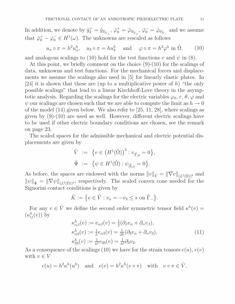
FRICTIONAL CONTACT OF AN ANISOTROPIC PIEZOELECTRIC PLATE 11
In addition, we denote by g+3 = g3|
Γ+
, ϕ+0 = ϕ0|
Γ+
, ϕ−0 = ϕ0|
Γ−and we assume
that ϕ+0 − ϕ−
0 ∈ H1(ω). The unknowns are rescaled as follows
uα π = h2uhα, u3 π = huh
3 and ϕ π = h3ϕh in Ω, (10)
and analogous scalings to (10) hold for the test functions v and ψ in (8).At this point, we briefly comment on the choice (9)-(10) for the scalings of
data, unknowns and test functions. For the mechanical forces and displace-ments we assume the scalings also used in [5] for linearly elastic plates. In[24] it is shown that these are (up to a multiplicative power of h) “the onlypossible scalings” that lead to a linear Kirchhoff-Love theory in the asymp-totic analysis. Regarding the scalings for the electric variables ϕ0, r, θ, ϕ andψ our scalings are chosen such that we are able to compute the limit as h→ 0of the model (14) given below. We also refer to [25, 11, 28], where scalings asgiven by (9)-(10) are used as well. However, different electric scalings haveto be used if other electric boundary conditions are chosen, see the remarkon page 23.
The scaled spaces for the admissible mechanical and electric potential dis-placements are given by
V :=
v ∈(
H1(Ω))3
: v|ΓD= 0
,
Ψ :=
ψ ∈ H1(Ω) : ψ|ΓeD= 0
.
As before, the spaces are endowed with the norms ‖v‖V = ‖∇v‖(L2(Ω))9 and
‖ψ‖Ψ = ‖∇ψ‖(L2(Ω))3, respectively. The scaled convex cone needed for the
Signorini contact conditions is given by
K :=
v ∈ V : vn = −v3 ≤ s on Γ−
.
For any v ∈ V we define the second order symmetric tensor field κh(v) =(κh
ij(v)) by
κhαβ(v) := eαβ(v) = 1
2(∂βvα + ∂αvβ),
κhα3(v) := 1
heα3(v) = 1
2h(∂3vα + ∂αv3),
κh33(v) := 1
h2e33(v) = 1h2∂3v3.
(11)
As a consequence of the scalings (10) we have for the strain tensors e(u), e(v)with v ∈ V
e(u) = h2κh(uh) and e(v) = h2κh(v π) with v π ∈ V .
12 I. N. FIGUEIREDO AND G. STADLER
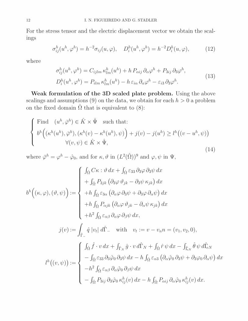
For the stress tensor and the electric displacement vector we obtain the scal-ings
σhij(u
h, ϕh) = h−2σij(u, ϕ), Dhi (u
h, ϕh) = h−2Dhi (u, ϕ), (12)
where
σhij(u
h, ϕh) = Cijlm κhlm(uh) + hPαij ∂αϕ
h + P3ij ∂3ϕh,
Dhi (u
h, ϕh) = Pilm κhlm(uh) − h εiα ∂αϕ
h − εi3 ∂3ϕh.
(13)
Weak formulation of the 3D scaled plate problem. Using the abovescalings and assumptions (9) on the data, we obtain for each h > 0 a problem
on the fixed domain Ω that is equivalent to (8):
Find (uh, ϕh) ∈ K × Ψ such that:
bh(
(κh(uh), ϕh), (κh(v) − κh(uh), ψ))
+ j(v) − j(uh) ≥ lh(
(v − uh, ψ))
∀(v, ψ) ∈ K × Ψ,(14)
where ϕh = ϕh − ϕ0, and for κ, ϑ in (L2(Ω))9 and ϕ, ψ in Ψ,
bh(
(κ, ϕ), (ϑ, ψ))
:=
∫
ΩCκ : ϑ dx+∫
Ω ε33 ∂3ϕ∂3ψ dx
+∫
Ω P3jk
(
∂3ϕϑjk − ∂3ψ κjk
)
dx
+h∫
Ω ε3α
(
∂αϕ∂3ψ + ∂3ϕ∂αψ)
dx
+h∫
Ω Pαjk
(
∂αϕϑjk − ∂αψ κjk
)
dx
+h2∫
Ω εαβ ∂αϕ∂βψ dx,
j(v) :=
∫
Γ−
q |vt| dΓ− with vt := v − vnn = (v1, v2, 0),
lh(
(v, ψ))
:=
∫
Ω f · v dx+∫
ΓNg · v dΓN +
∫
Ω r ψ dx−∫
ΓeNθ ψ dΓeN
−∫
Ω ε33 ∂3ϕ0 ∂3ψ dx− h∫
Ω εα3
(
∂αϕ0 ∂3ψ + ∂3ϕ0 ∂αψ)
dx
−h2∫
Ω εαβ ∂αϕ0 ∂βψ dx
−∫
Ω P3ij ∂3ϕ0 κhij(v) dx− h
∫
Ω Pαij ∂αϕ0 κhij(v) dx.
FRICTIONAL CONTACT OF AN ANISOTROPIC PIEZOELECTRIC PLATE 13
Using the relation (11) between κh(v) and v, in the sequel (mainly in theproof of Theorem 1), we abbreviate
bh(
(κh(uh), ϕ), (κh(v), ψ))
by bh(
(uh, ϕ), (v, ψ))
.
In contrast to (8), where the dependence on the parameter h is implicit (bymeans of the domain Ω), problem (14) now depends explicitly on h, but isdefined on a domain independent of h.
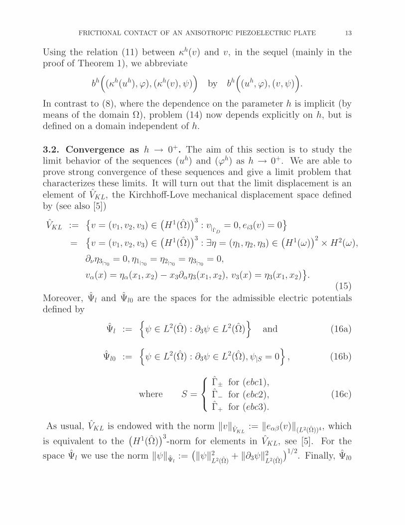
3.2. Convergence as h → 0+. The aim of this section is to study thelimit behavior of the sequences (uh) and (ϕh) as h → 0+. We are able toprove strong convergence of these sequences and give a limit problem thatcharacterizes these limits. It will turn out that the limit displacement is anelement of VKL, the Kirchhoff-Love mechanical displacement space definedby (see also [5])
VKL :=
v = (v1, v2, v3) ∈(
H1(Ω))3
: v|ΓD
= 0, ei3(v) = 0
=
v = (v1, v2, v3) ∈(
H1(Ω))3
: ∃η = (η1, η2, η3) ∈(
H1(ω))2 ×H2(ω),
∂νη3|γ0= 0, η1|γ0
= η2|γ0= η3|γ0
= 0,
vα(x) = ηα(x1, x2) − x3∂αη3(x1, x2), v3(x) = η3(x1, x2)
.
(15)
Moreover, Ψl and Ψl0 are the spaces for the admissible electric potentialsdefined by
Ψl :=
ψ ∈ L2(Ω) : ∂3ψ ∈ L2(Ω)
and (16a)
Ψl0 :=
ψ ∈ L2(Ω) : ∂3ψ ∈ L2(Ω), ψ|S = 0
, (16b)
where S =
Γ± for (ebc1),
Γ− for (ebc2),
Γ+ for (ebc3).
(16c)
As usual, VKL is endowed with the norm ‖v‖VKL:= ‖eαβ(v)‖(L2(Ω))4, which
is equivalent to the(
H1(Ω))3
-norm for elements in VKL, see [5]. For the
space Ψl we use the norm ‖ψ‖Ψl:=
(
‖ψ‖2L2(Ω)
+ ‖∂3ψ‖2L2(Ω)
)1/2. Finally, Ψl0
14 I. N. FIGUEIREDO AND G. STADLER
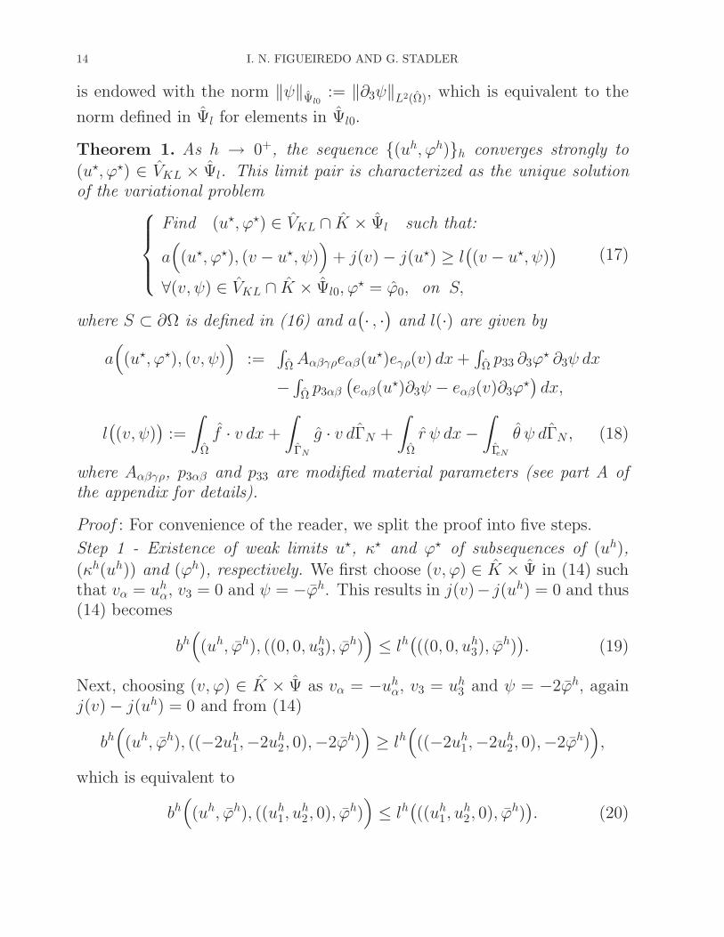
is endowed with the norm ‖ψ‖Ψl0:= ‖∂3ψ‖L2(Ω), which is equivalent to the
norm defined in Ψl for elements in Ψl0.
Theorem 1. As h → 0+, the sequence (uh, ϕh)h converges strongly to
(u⋆, ϕ⋆) ∈ VKL × Ψl. This limit pair is characterized as the unique solutionof the variational problem
Find (u⋆, ϕ⋆) ∈ VKL ∩ K × Ψl such that:
a(
(u⋆, ϕ⋆), (v − u⋆, ψ))
+ j(v) − j(u⋆) ≥ l(
(v − u⋆, ψ))
∀(v, ψ) ∈ VKL ∩ K × Ψl0, ϕ⋆ = ϕ0, on S,
(17)
where S ⊂ ∂Ω is defined in (16) and a(
· , ·)
and l(·) are given by
a(
(u⋆, ϕ⋆), (v, ψ))
:=∫
ΩAαβγρeαβ(u⋆)eγρ(v) dx+∫
Ω p33 ∂3ϕ⋆ ∂3ψ dx
−∫
Ω p3αβ
(
eαβ(u⋆)∂3ψ − eαβ(v)∂3ϕ⋆)
dx,
l(
(v, ψ))
:=
∫
Ω
f · v dx+
∫
ΓN
g · v dΓN +
∫
Ω
r ψ dx−∫
ΓeN
θ ψ dΓN , (18)
where Aαβγρ, p3αβ and p33 are modified material parameters (see part A ofthe appendix for details).
Proof : For convenience of the reader, we split the proof into five steps.
Step 1 - Existence of weak limits u⋆, κ⋆ and ϕ⋆ of subsequences of (uh),
(κh(uh)) and (ϕh), respectively. We first choose (v, ϕ) ∈ K × Ψ in (14) suchthat vα = uh
α, v3 = 0 and ψ = −ϕh. This results in j(v)− j(uh) = 0 and thus(14) becomes
bh(
(uh, ϕh), ((0, 0, uh3), ϕ
h))
≤ lh(
((0, 0, uh3), ϕ
h))
. (19)
Next, choosing (v, ϕ) ∈ K × Ψ as vα = −uhα, v3 = uh
3 and ψ = −2ϕh, againj(v) − j(uh) = 0 and from (14)
bh(
(uh, ϕh), ((−2uh1,−2uh
2, 0),−2ϕh))
≥ lh(
((−2uh1,−2uh
2, 0),−2ϕh))
,
which is equivalent to
bh(
(uh, ϕh), ((uh1, u
h2, 0), ϕh)
)
≤ lh(
((uh1, u
h2, 0), ϕh)
)
. (20)
FRICTIONAL CONTACT OF AN ANISOTROPIC PIEZOELECTRIC PLATE 15
Adding (19) and (20) results in
bh(
(uh, ϕh), (uh, ϕh))
≤ lh(
(uh, ϕh))
,
from which we can deduce
‖uh‖2V+
∫
Ω
κh(uh) : κh(uh)dx+‖h ∂1ϕh‖2
L2(Ω)+‖h ∂2ϕ
h‖2L2(Ω)
+‖∂3ϕh‖2
L2(Ω)< c,
(21)where c > 0 is a constant independent of h (see also [28]). Consequently,there are weakly convergent subsequences of (uh), (κh(uh)) and (ϕh) with
uh u⋆ in(
H1(Ω))3,
κh(uh) κ⋆ in(
L2(Ω))9,
ϕh ϕ⋆ = ϕ⋆ − ϕ0 in L2(Ω),
ϕh ϕ⋆ in L2(Ω),
(h∂1ϕh, h∂2ϕ
h, ∂3ϕh) (0, 0, ∂3ϕ
⋆) in(
L2(Ω))3.
(22)
The first two weak convergences follow directly from (21). The existence ofthe third and fourth weak limit in (22) follows from (21) using the fact that
ϕh(x1, x2, x3) =
∫ x3
−1 ∂3ϕh(x1, x2, y3)dy3 for S = Γ± or S = Γ−
−∫ +1
x3∂3ϕ
h(x1, x2, y3)dy3 for S = Γ+,(23)
which results in
‖ϕh‖L2(Ω) ≤√
2 ‖∂3ϕh(x1, x2, x3)‖L2(Ω) ≤ c (24)
with c > 0 independent of h. This implies the L2(Ω)-boundedness of ϕh and
ϕh = ϕh + ϕ0. In particular, ϕ⋆ = ϕ0 on S because ϕh = 0 on ΓeD ⊇ S.Finally, the last convergence in (22) is a consequence of (21), which impliesthat
(h∂1ϕh, h∂2ϕ
h, ∂3ϕh) (ϑ1, ϑ2, ϑ3) in
(
L2(Ω))3.
The weak convergence of ϕh to ϕ⋆ yields ∂iϕh ∂iϕ
⋆ in L2(Ω), and thusϑα = 0 for α = 1, 2, and ϑ3 = ∂3ϕ
⋆.Moreover, from (22) we can also deduce that u⋆ ∈ VKL. In fact, from
(21) we obtain boundedness of the sequence κhi3(u
h) in L2(Ω). Consequently,
eα3(uh) = hκh
α3(uh) and e33(u
h) = h2κh33(u
h) → 0 strongly in L2(Ω). Thus,
16 I. N. FIGUEIREDO AND G. STADLER
ei3(u⋆) := 1
2(∂iu⋆3 + ∂3u
⋆i ) = 0, which implies u⋆ ∈ VKL. We also remark that,
appropriate choice of subsequences guarantees that
κ⋆αβ = eαβ(u⋆) =
1
2(∂αu
⋆β + ∂βu
⋆α) (25)
yielding that the weak limit κ⋆ depends explicitly on u⋆.
Step 2 - Auxiliary limits. As a consequence of the weak convergences (22)
we obtain for arbitrary (v, ψ) ∈ VKL × Ψ that
limh→0+
bh(
(uh, ϕh), (v, ψ))
:= b⋆(
(u⋆, ϕ⋆), (v, ψ))
,
limh→0+
lh(
(v, ψ)
) := l⋆(
(v, ψ)
),
where for (v, ψ) in VKL × Ψ
b⋆(
(u⋆, ϕ⋆), (v, ψ))
:=∫
ΩCαβijκ⋆ijeαβ(v) dx+
∫
Ω ε33 ∂3ϕ⋆ ∂3ψ dx+
+∫
Ω P3αβ ∂3ϕ⋆ eαβ(v) dx−
∫
Ω P3lm ∂3ψ κ⋆lm dx,
(26)and
l⋆(
(v, ψ)
) :=∫
Ω f · v dx+∫
ΓNg · v dΓN +
∫
Ω r ψ dx−∫
ΓeNθ ψ dΓN
−∫
Ω ε33 ∂3ϕ0 ∂3ψ dx−∫
Ω P3αβ ∂3ϕ0 eαβ(v) dx.
Moreoverlim
h→0+
(
j(v) − j(uh))
= j(v) − j(u⋆).
Step 3 - The weak limits u⋆, κ⋆ and ϕ⋆ are also strong limits. Here, it sufficesto prove that χh strongly converges to χ⋆ in (L2(Ω))12, with
χh = (κh(uh), h∂1ϕh, h∂2ϕ
h, ∂3ϕh) ∈
(
L2(Ω))12
χ⋆ = (κ⋆, 0, 0, ∂3ϕ⋆) ∈
(
L2(Ω))12.
By the ellipticity and linearity of bh(. , .), we have
c‖χh − χ⋆‖2(L2(Ω))12
≤ bh(
(κh(uh) − κ⋆, ϕh − ϕ⋆), (κh(uh) − κ⋆, ϕh − ϕ⋆))
= bh(
(κh(uh), ϕh), (κh(uh), ϕh))
+ bh(
(κ⋆, ϕ⋆), (κ⋆, ϕ⋆))
−bh(
(κh(uh), ϕh), (κ⋆, ϕ⋆))
− bh(
(κ⋆, ϕ⋆), (κh(uh), ϕh))
,
(27)
FRICTIONAL CONTACT OF AN ANISOTROPIC PIEZOELECTRIC PLATE 17
where c > 0 is independent of h. Replacing ψ by ψ − ϕh in (14), we obtain
bh(
(κh(uh), ϕh), (κh(v)−κh(uh), ψ−ϕh))
+ j(v)− j(uh) ≥ lh(
v−uh, ψ−ϕh)
,
which is, recalling that ϕh = ϕh − ϕ0 and noticing that (κh(v)− κh(uh), ψ−ϕh) = (κh(v), ψ) − (κh(uh), ϕh), equivalent to
bh(
(κh(uh), ϕh), (κh(uh), ϕh))
≤ bh(
(κh(uh), ϕh), (κh(v), ψ))
+ j(v) − j(uh)
−∫
Ω f · (v − uh) dx−∫
ΓNg · (v − uh) dΓN
−∫
Ω r (ψ − ϕh) dx+∫
ΓeNθ (ψ − ϕh) dΓeN ,
(28)
for any v ∈ K. Thus, considering v ∈ VKL ∩ K in (14), using the weakconvergences (22) and the limits of step 2, we derive from (27) and (28) theestimate
c lim sup ‖χh − χ⋆‖2(L2(Ω))12
≤ b⋆(
(u⋆, ϕ⋆), (v, ψ))
+ j(v) − j(u) − l(v − u⋆, ψ − ϕ⋆) − b⋆(
(u⋆, ϕ⋆), (u⋆, ϕ⋆))
= b⋆(
(u⋆, ϕ⋆), (v − u⋆, ψ − ϕ⋆))
+ j(v) − j(u⋆) − l(v − u⋆, ψ − ϕ⋆),
with l(.) as defined in (18). Choosing v = u⋆ and ψ = ϕ⋆ in the aboveestimate yields
c lim sup ‖χh − χ⋆‖(L2(Ω))12 ≤ 0,
which implies the strong convergence of χh to χ⋆ in (L2(Ω))12. Due to ∂3(ϕh−
ϕ⋆) → 0 strongly in L2(Ω) and ϕh−ϕ⋆ ∈ Ψl0, we obtain ϕh−ϕ⋆ → 0 strongly
in L2(Ω) using the equivalence of the norms ‖.‖Ψland ‖.‖Ψl0
in Ψl0. Moreover,
ei3(u⋆) = 0, eαβ(u⋆) = κ⋆
αβ and κh(uh) → κ⋆ strongly in (L2(Ω))9. Thus, we
have eαβ(uh) → eαβ(u⋆) strongly in (L2(Ω))9, which proves that uh → u⋆
strongly in (H1(Ω))3.
Step 4 - Formulas for κ⋆ = (κ⋆ij). In (25) we already observed that κ⋆
αβ =
eαβ(u⋆). To obtain formulas for κ⋆α3 and κ⋆
33, we first multiply (14) by h2 andconsider ψ = 0. Next, we multiply (14) by h and consider v3 = uh
3 and ψ = 0.Due to the strong convergences proved in step 3, as h→ 0+ the limit in the
18 I. N. FIGUEIREDO AND G. STADLER
two resulting variational inequalities exists and we obtain∫
Ω
(
Cij33 κ⋆ij + P333 ∂3ϕ
⋆)
∂3(v3 − u⋆3) dx ≥ 0 (29a)
∀v3 ∈ H1(Ω), v3|Γ−≥ −s, v3|ΓD
= 0,
∫
Ω
(
Cijα3 κ⋆ij + P3α3 ∂3ϕ
⋆)
∂3(vα − u⋆α) dx ≥ 0 (29b)
∀vα ∈ H1(Ω), vα|ΓD= 0.
Since u⋆3 is independent of x3, we obtain ∂3u
⋆3 = 0 in (29a). In (29b), we
choose vα := zα + u⋆α with zα ∈ H1(Ω) arbitrary with zα|ΓD
= 0. Hence, the
inequalities (29) become∫
Ω
(
Cij33 κ⋆ij + P333 ∂3ϕ
⋆)
∂3v3 dx ≥ 0 (30a)
∀v3 ∈ H1(Ω), v3|Γ−≥ −s, v3|ΓD
= 0,
∫
Ω
(
Cijα3 κ⋆ij + P3α3 ∂3ϕ
⋆)
∂3vα dx = 0 (30b)
∀vα ∈ H1(Ω), vα|ΓD= 0.
For arbitrary θ ∈ D(Ω) we consider v3 in (30a) as
v3(x1, x2, x3) =∫ x3
−1 θ(x1, x2, t) dt+ z3(x1, x2),
with z3 ∈ H1(ω) such that z3(x1, x2) ≥ −s(x1, x2,−1) for all (x1, x2) ∈ ω.Moreover, we choose vα in (30b) as
vα(x1, x2, x3) =
∫ x3
−1
θ(x1, x2, t) dt.
Then, from (30) we obtain
Cij33 κ⋆ij + P333 ∂3ϕ
⋆ = 0 in L2(Ω),
Cijα3 κ⋆ij + P3α3 ∂3ϕ
⋆ = 0 in L2(Ω).(31)
FRICTIONAL CONTACT OF AN ANISOTROPIC PIEZOELECTRIC PLATE 19
Since κ⋆αβ = eαβ(u⋆), this leads to the formulas
κ⋆α3 = −1
2bνα
(
aνρβeρβ(u⋆) + cν∂3ϕ
⋆)
κ⋆33 = − 1
C3333
(
P333∂3ϕ⋆ + C33αβeαβ(u⋆)
)
+ C33α3
C3333bνα
(
aνρβeρβ(u⋆) + cν∂3ϕ⋆)
(32)where the coefficients bνα, aνρβ and cν are modified material parameters de-fined in part A of the appendix.
Step 5 - The limit variational inequality. From the previous steps 3-4 and (13)
we directly obtain the following strong L2(Ω)-convergences, for the scaledstress tensor and the electric displacement vector
σhij(u
h, ϕh) → σ⋆ij and Dh
i (uh, ϕh) → D⋆
i
whereσ⋆
αβ = Cαβlmκ⋆lm + P3αβ∂3ϕ
⋆
σ⋆i3 = Ci3lmκ
⋆lm + P3i3∂3ϕ
⋆ = 0 (because of (31))
D⋆i = Pilmκ
⋆lm − εi3∂3ϕ
⋆.
(33)
With (32) for κ⋆ we get
σ⋆αβ = Aαβγρeαβ(u⋆) + p3αβ∂3ϕ
⋆
D⋆i = piαβeαβ(u⋆) − pi3∂3ϕ
⋆,(34)
where the coefficients Aαβγρ, piαβ and pi3 are defined in the appendix, partA.
Using again the strong convergences obtained in step 3 and ϕ⋆ = ϕ⋆ + ϕ0
we can take the limit in (14) and obtain the limit variational inequality:
Find (u⋆, ϕ⋆) ∈ VKL ∩ K × Ψl such that:
b⋆(
(u⋆, ϕ⋆), (v − u⋆, ψ))
+ j(v) − j(u⋆) ≥ l(
(v − u⋆, ψ))
∀(v, ψ) ∈ VKL ∩ K × Ψl0, ϕ⋆ = ϕ0 on S.
(35)
Here the linear form l(·) is defined by (18) and the bilinear form b⋆(· , ·) by(26). From (33) one obtains
b⋆(
(u⋆, ϕ⋆), (v, ψ))
=
∫
Ω
σ⋆αβ eαβ(v) dx−
∫
Ω
D⋆3 ∂3ψ dx. (36)
Using now the equivalent definitions of σ⋆αβ and D⋆
3 given in (34), the right-
hand side of (36) turns out to be precisely a(
(u⋆, ϕ⋆), (v, ψ))
. Hence (35)
20 I. N. FIGUEIREDO AND G. STADLER
coincides with the limit problem (17) and the proof of the theorem is finished.We remark that, the solution of this limit problem is unique if the bilinearform a
(
· , ·)
in (17) is elliptic in the set VKL ∩ K × Ψl0 (cf. [14]). Thisis, for instance, the case if the material is mechanically monoclinic, thatis, Cαβγ3 = 0 = Cα333 (see Theorem 3.3 in [11]). One easily verifies thatthis ellipticity result also holds true for a laminated plate with mechanicallymonoclinic piezoelectric layers.
3.3. Rescaling to the original domain. The limit variational inequality(17) can be rescaled to the original plate Ω = ω× (−h, h). In order to do so,let x3 ∈ (−1,+1) and u⋆
α = ζ⋆α − x3∂αζ
⋆3 , u
⋆3 = ζ⋆
3 be the components of theKirchhoff-Love limit displacement u⋆. The corresponding descaled functionζ = (ζ1, ζ2, ζ3) is given by
ζα := h2ζ⋆α, ζ3 := h ζ⋆
3 in ω,
which leads to the descaled variables
uα(x) := h2u⋆α = ζα(x1, x2) − x3∂αζ3(x1, x2),
u3(x) := hu⋆3(x1, x2) = ζ3(x1, x2),
ϕ(x) := h3ϕ⋆(x),
for x = (x1, x2, x3) ∈ Ω = ω × (−h, h). Above, ζα and ζ3 are in-plane andtransverse Kirchhoff-Love displacements, ui is the limit mechanical displace-ments and ϕ the electric potential inside the plate Ω. The spaces VKL, Ψl
and Ψl0 correspond to the descaled variables defined over Ω and are given by(15)–(16) with Ω replaced by Ω and Γ by Γ in the definition of S.
Plugging the rescaled variables in the limit problem found in Theorem 1,we obtain the following rescaled limit problem:
Find (u, ϕ) ∈ VKL ∩K × Ψl such that:
a(
(u, ϕ), (v− u, ψ))
+ j(v) − j(u) ≥ l(
(v − u, ψ))
, ∀(v, ψ) ∈ VKL ∩K × Ψl0,
ϕ = ϕ0, on S,
(37)where for u, v in VKL and ϕ, ψ in Ψ
a(
(u, ϕ), (v, ψ))
:=∫
ΩAαβγρeαβ(u)eγρ(v) dx+∫
Ω p33 ∂3ϕ∂3ψ dx
−∫
Ω p3αβ
(
eαβ(u) ∂3ψ − eαβ(v) ∂3ϕ)
dx,
FRICTIONAL CONTACT OF AN ANISOTROPIC PIEZOELECTRIC PLATE 21
and
l(
(v, ψ))
:=
∫
Ω
f · v dx+
∫
ΓN
g · v dΓN +
∫
Ω
r ψ dx−∫
ΓeN
θ ψ dΓeN .
3.4. Decoupling of u and ϕ. The structure of the bilinear form a(· , ·),obtained by the asymptotic procedure above allows a certain uncouplingof the mechanical displacement u and the electric potential ϕ. This leadsto a variational inequality in the mechanical displacement u only, and anexplicit formula for the electric potential. This explicit form, which is asecond order polynomial with coefficients that depend on the Kirchhoff-Lovedisplacement u, obeys a slightly different form for each of the boundarypartitions (ebc1), (ebc2), (ebc3) for the electric data.
To derive the decoupling, we choose v = u in the variational inequality(37) and obtain
∫
Ω
(
p33 ∂3ϕ− p3αβ eαβ(u))
∂3ψ dx =
∫
Ω
r ψ dx−∫
ΓeN
θ ψ dΓeN
for all ψ ∈ Ψl0. Due to the density of Ψl0 in D(Ω) (see [28]), this yields thefollowing formula for ∂3ϕ
∂3ϕ =p3αβ
p33
(
eαβ(ζ) − x3 ∂αβζ3)
− d
p33with d = P3r + c, (38)
where c ∈ D(ω) and P3r =∫ x3
−h r dy3 denotes the antiderivative of r withrespect to the thickness variable x3. Using this latter formula and one ofthe boundary conditions (ebci), we obtain explicit formulas for the electricpotential. In the case that the electric potential is given on both the upperand lower surface Γ− and Γ+, we integrate (38) with respect to x3. Then,using the given boundary data, we obtain the formula (see also Theorem 2.1in [8])
ϕ(x1, x2, x3) = ϕ−0 (x1, x2) +
∫ x3
−h
(
(p3αβ
p33− aαβ
p33c0
)
eαβ(ζ)
−(p3αβ
p33y3 −
bαβ
p33c0
)
∂αβζ3 +(ϕ+
0 − ϕ−0 + R) c0 − P3r
p33
)
dy3,
(39)
22 I. N. FIGUEIREDO AND G. STADLER
where
aαβ :=
∫ +h
−h
p3αβ
p33dx3, bαβ :=
∫ +h
−h
x3p3αβ
p33dx3,
c0 =(
∫ +h
−h
1
p33dx3
)−1
, R :=
∫ +h
−h
P3r
p33dx3.
For the case that the electric potential is either given on Γ− or Γ+, i.e., forthe cases (ebc2) and (ebc3), we plug (38) into (37) and choose again v = u
to obtain
−∫
Ω
(P3r + c) ∂3ψ dx =
∫
Ω
r ψ dx−∫
ΓeN
θ ψ dΓeN .
¿From the Green formula we obtain ∂3(P3r + c) = r in D(Ω) and
−∫
ΓeN
(P3r + c)n3ψ dx−∫
ΓeD
(P3r + c)n3ψ dx = −∫
ΓeN
θ ψ dΓeN , (40)
with n3 = 0 on the lateral boundaries Γe and Γs, n3 = ±1 on Γ± and ψ = 0on ΓeD. Choosing ψ such that ψ = 0 on the lateral boundary, (40) reduces to
∫
Γ+
(P3r + c)ψ dΓ+ =
∫
Γ+
θ ψ dΓ+ for (ebc2),
−∫
Γ−
(P3r + c)ψ dΓ− =
∫
Γ−
θ ψ dΓ− for (ebc3).
This implies, for (ebc2) that c(x1, x2) = (θ − P3r)(x1, x2,+h), and for (ebc3)that c(x1, x2) = (−θ − P3r)(x1, x2,−h). Consequently, integrating (38) withd = P3r + c along the thickness variable (from −h to x3 for (ebc2) and fromx3 to +h for (ebc3)), we obtain
ϕ(x1, x2, x3) = ϕ−0 (x1, x2) +
∫ x3
−h
p3αβ
p33
(
eαβ(ζ) − y3 ∂αβζ3)
dy3
−∫ x3
−h
P3r(x1, x2, y3) + (θ − P3r)(x1, x2,+h)
p33dy3 for (ebc2)
(41)
FRICTIONAL CONTACT OF AN ANISOTROPIC PIEZOELECTRIC PLATE 23
and
ϕ(x1, x2, x3) = ϕ+0 (x1, x2) −
∫ +h
x3
p3αβ
p33
(
eαβ(ζ) − y3 ∂αβζ3)
dy3
+
∫ +h
x3
P3r(x1, x2, y3) + (−θ − P3r)(x1, x2,−h)p33
dy3 for (ebc3).
(42)Next, we plug the above explicit forms for the electric potential into (37) andchoose the electric test function ψ = 0. This gives an equivalent formulationfor the variational inequality (37), which is summarized in the next theorem.Now, the mechanical displacement and the electric potential are not coupledin the variational inequality any more. The main advantage of this decoupledformulation is that after solving a variational inequality for the mechanicaldisplacement, one can use an explicit formula for the electric potential.
Theorem 2. Let (u, ϕ) ∈ VKL × Ψl be a solution of problem (37), whereuα = ζα − x3∂αζ3, u3 = ζ3, and ζ = (ζ1, ζ2, ζ3). Then the Kirchhoff-Lovemechanical displacement u ∈ VKL is also characterized as solution of thevariational inequality
Find u ∈ VKL ∩K such that:
aebci(u, v − u) + j(v) − j(u) ≥ lebci(v − u) ∀v ∈ VKL ∩K,(43)
and the electric potential can be derived a posteriori from (39) for (ebc1),(41) for (ebc2) and (42) for (ebc3). The modified bilinear and linear forms,respectively aebci(·, ·) and lebci(·), are defined by
aebci(u, v) :=
∫
ω
(
N ebciαβ (u) eαβ(η) +M ebci
αβ (u) ∂αβη3
)
dω,
lebci(v) :=
∫
Ω
f · v dΩ +
∫
ΓN
g · v dΓN + lebcie (v),
where N ebciαβ (u), N ebci
αβ (u) and lebcie (.) are detailed in part B of the appendix.
Remark 1. Let us comment on a different (fourth) choice of electric bound-ary condition (ebc4) given by
(ebc4) : ΓeN = Γs ∪ Γ− ∪ Γ+ and ΓeD = Γe
where we assume meas(γe) > 0. This means that we apply an electric sur-face charge on both the upper and lower surface of the plate. This case
24 I. N. FIGUEIREDO AND G. STADLER
requires a different treatment in the asymptotic analysis: Note that instead
of (22) we only obtain uh u⋆ in(
H1(Ω))3
, κh(uh) κ⋆ in(
L2(Ω))9
and
(h∂1ϕh, h∂2ϕ
h, ∂3ϕh) (ϑ1, ϑ2, ϑ3) in
(
L2(Ω))3
. Now, we cannot conclude
that ϕh, ϕh are weakly convergent since (23) and consequently (24) do notapply. Hence, ϑ1, ϑ2 are not necessary equal to zero and the limit problemchanges considerably. This is in accordance with observations in [26, 25, 33],where it is shown that for different electric boundary conditions significantlydifferent limit problems may arise. To obtain an easier interpretation for thelimit problem in case of (ebc4), it might be advantageous to consider scalingsdifferent from those used in this paper for the electric potential.
Remark 2. We now sketch the strong (i.e., the differential) form of thelimit problem obtained in Theorem 2. This form uses Lagrange multipliers toresolve the contact and friction conditions and is obtained assuming sufficientregularity of (u, ϕ) as well as partial integration. It follows from dualitytheory [10] that there exist so called multipliers (or dual variables) (λ, µ) ∈(H2(ω))′ × (L2(ω))2 satisfying complementarity conditions (see (47d), (47e)below) for (43), where (H2(ω))′ denotes the dual of H2(ω). Then, u ∈ VKL∩K can be written as
aebci(u, v) +
∫
Γ−
λ vn dΓ− +
∫
Γ−
µ · vt dΓ− = lebci(v), ∀v ∈ VKL. (44)
Choosing test functions v = (η1 − x3∂1η3, η2 − x3∂2η3, η3) ∈ VKL with η1 =η2 = 0 and η3 6= 0, i.e., v = (−x3∂1η3,−x3∂2η3, η3), (44) is equivalent to
∫
ω
M ebciαβ (u) ∂αβη3 −
∫
Γ−
λ η3 dΓ− +
∫
Γ−
µα (−x3∂αη3) dΓ− =
lebci(
(−x3∂1η3,−x3∂2η3, 0))
∀η3 ∈ H2(ω) with η3 = 0 on γ0.
(45)
On the other hand, choosing η3 = 0 and ηα 6= 0 for α = 1, 2, i.e., v =(η1, η2, 0), (44) becomes
∫
ω
N ebciαβ (u) eαβ(η) +
∫
Γ−
µα ηα dΓ− = lebci(
(η1, η2, 0))
∀(η1, η1) ∈(
H1(ω))2
with ηα = 0 on γ0.
(46)
Using Green’s theorem in (45) and (46) while neglecting regularity issues,and stating the complementarity conditions satisfied by (λ, µ) leads to thefollowing strong formulation of the limit problem.
FRICTIONAL CONTACT OF AN ANISOTROPIC PIEZOELECTRIC PLATE 25
Equilibrium equations (coupling mechanical and electric effects)[
∂αβMebciαβ (u) − λ+ hx3 ∂αµα = F ebci
3 in ω,
−∂αNebciαβ (u) + µβ = F ebci
β on ω, and β = 1, 2.(47a)
Boundary conditions[
ζ3 = 0 = ζ3
∂n, (ζ1, ζ2) = (0, 0) on γ0,
boundary conditions for the terms M ebciαβ + µα and N ebci
αβ .(47b)
Constitutive equations[
σαβ(u, ϕ) = Aαβγρeγρ(u) + p3αβ∂3ϕ, σi3(u, ϕ) = 0 in Ω,
Di(u, ϕ) = piαβeαβ(u) − pi3∂3ϕ in Ω.(47c)
Contact condition
un = −u3 =≤ s, λ ≥ 0, λ(un − s) = 0 on Γ−. (47d)
Friction condition
|µ| =√
µ21 + µ2
2 ≤ q and
|µ| < q ⇒ ut = 0,
|µ| = q ⇒ ∃c ≥ 0 : ut = cµ
on Γ−. (47e)
The terms F ebci3 and F ebci
β represent the transverse and tangential forcesacting on the middle plane ω of the plate. They are related to the mechanicalforces, electric data and charges appearing in the definition of the linear formlebci(·) (see part C of the appendix for details).
We observe that the limit mechanical displacement u satisfies a system ofequations independent of ϕ but depending on the elastic and piezoelectriccoefficients as well as the mechanical and electric data and boundary condi-tions. Moreover, (u, ϕ) also satisfies the limit constitutive equations (47c),which are a consequence of (34) and the descalings. In the equations (47a),the tangential and transverse displacements ζα and ζ3 are coupled due to the
26 I. N. FIGUEIREDO AND G. STADLER
anisotropy of the material (as can be seen in the definitions of M ebciαβ (u) and
N ebciαβ (u)) and since to the friction condition (the Lagrange multiplier µ ap-
pears in both equations of (47a)).For the case of a homogeneous and isotropic material and if we neglect
friction, the tangential and transverse displacements ζα and ζ3 decouple inthe asymptotic model. This happens since the equations in (47a) becomeindependent from each other since the friction terms containing µ vanish,since M ebci
αβ (u) = M ebciαβ (ζ3) only depends on ζ3 and N ebci
αβ (u) = N ebciαβ (ζ1, ζ2)
only depends on (ζ1, ζ2), see also [8, 11].
Remark 3. Obviously, the derivations in this paper remain true for friction-less unilateral contact. In the same way, the results hold for bilateral contactproblems (i.e. the contact region is known a priori) with Tresca friction,which is physically more meaningful than unilateral (i.e. unknown) contactwith Tresca friction. However, for the realization of contact with Coulombfriction (which is a realistic and usually used friction law, see also the nextsection) often a sequence of Tresca friction problems is solved. This rendersunilateral contact with Tresca friction to an important problem as well.
It should be mentioned that the asymptotic procedure employed in this pa-per applies in a similar way to contact problems with thin linear elastic plateswith integrated piezoelectric patches or layers. The corresponding asymptoticmodels can be derived using the same arguments as in this paper, providedthe piezoelectric patches or layers are perfectly linked (surface bonded or em-bedded) to the elastic plates.
4. Numerical Examples
Here, we present numerical tests for the asymptotic equations obtained inthe previous sections. We first use a simple example to verify our code andto discuss the friction and contact conditions and then focus on two exam-ples, where the mechanical frictional contact behavior interacts significantlywith the electric potential. The numerical treatment of the contact and fric-tion conditions for the mechanical displacement follows [16]. The mechanicalequations are discretized with bilinear finite elements for the tangential com-ponents ζ1 and ζ2 and with second-order elements for ζ3. Note that, whilethe asymptotic equations are defined on a two-dimensional domain, the fric-tional contact conditions remain structurally as in three-dimensional contact
FRICTIONAL CONTACT OF AN ANISOTROPIC PIEZOELECTRIC PLATE 27
mechanics, where frictional contact occurs on two-dimensional boundary sur-faces. To slightly simplify the problem we replace for our numerical imple-mentation the contact and friction conditions on Γ− by the same conditionsin the middle plane (and, for consistency, we also elevate the obstacle by h).
In all our examples we consider a laminated plate made of two layers ofdifferent PZT piezoelectric ceramic materials. The material parameters aretaken from the tables VIII and XI in [19]. Both layers are assumed to be ofthe same thickness h = 0.01 leading to a plate of thickness 0.02. The dataare given in SI units, i.e., length is measured in meter, mechanical forces inNewton and electrical potentials in Volt.
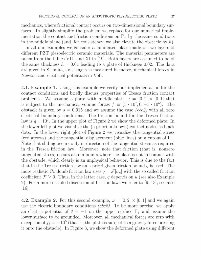
4.1. Example 1. Using this example we verify our implementation for thecontact conditions and briefly discuss properties of Tresca friction contactproblems. We assume a plate with middle plate ω = [0, 2] × [0, 1] thatis subject to the mechanical volume forces f ≡ (5 · 107, 0,−5 · 105). Theobstacle is given by s = 0.015 and we assume the case (ebc2) with all zeroelectrical boundary conditions. The friction bound for the Tresca frictionlaw is q = 107. In the upper plot of Figure 2 we show the deformed plate. Inthe lower left plot we visualize the (a priori unknown) contact nodes as blackdots. In the lower right plot of Figure 2 we visualize the tangential stress(red arrows) and the tangential displacement (blue lines) on a cutout of Γ−.Note that sliding occurs only in direction of the tangential stress as requiredin the Tresca friction law. Moreover, note that friction (that is, nonzerotangential stress) occurs also in points where the plate is not in contact withthe obstacle, which clearly is an unphysical behavior. This is due to the factthat in the Tresca friction law an a priori given friction bound q is used. Themore realistic Coulomb friction law uses q = F|σn| with the so called frictioncoefficient F ≥ 0. Thus, in the latter case, q depends on u (see also Example2). For a more detailed discussion of friction laws we refer to [9, 13], see also[16].
4.2. Example 2. For this second example, ω = [0, 2] × [0, 1] and we againuse the electric boundary conditions (ebc2). To be more precise, we applyan electric potential of θ = −1 on the upper surface Γ+ and assume thelower surface to be grounded. Moreover, all mechanical forces are zero withexception of f3 ≡ −105 (that is, the plate is subject to a gravity force pressingit onto the obstacle). In Figure 3, we show the deformed plate using different

28 I. N. FIGUEIREDO AND G. STADLER
0 0.2 0.4 0.6 0.8 1 1.2 1.4 1.6 1.8 2
0
0.1
0.2
0.3
0.4
0.5
0.6
0.7
0.8
0.9
1
0.4 0.5 0.6 0.7 0.8 0.9 10.4
0.5
0.6
0.7
0.8
0.9
1
Figure 2. Example 1: Deformed plate (upper plot). Lowerplots: nodes where the plate is in contact with the rigid obstacle(black dots in left plot); tangential displacement (blue lines inright plot) and tangential stress (red arrows in right plot) on apart of ω.
obstacles. Besides the Signorini contact conditions, we use the Coulombfriction law since it is more realistic than the Tresca law. Coulomb frictionmeans that q is not given a priori, but that q = F|σn|, with F ≥ 0 (we useF = 1). The Coulomb friction problem is numerically treated by solving asequence of Tresca friction problems, see [16]. The computations shown inFigure 3 are done using 80 × 40 finite elements.
Remarkably, the region of actual contact between obstacle and plate isrelatively small, even though additionally to the applied electric potentialthe plate is subject to a gravity force pressing it towards the obstacle: Fors ≡ 0.015, contact occurs only on 4 grid points. For the two other obstacle
FRICTIONAL CONTACT OF AN ANISOTROPIC PIEZOELECTRIC PLATE 29
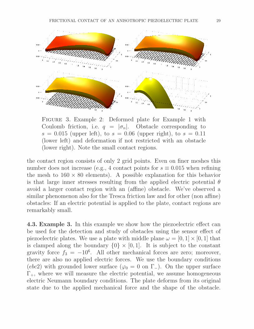
Figure 3. Example 2: Deformed plate for Example 1 withCoulomb friction, i.e. q = |σn|. Obstacle corresponding tos = 0.015 (upper left), to s = 0.06 (upper right), to s = 0.11(lower left) and deformation if not restricted with an obstacle(lower right). Note the small contact regions.
the contact region consists of only 2 grid points. Even on finer meshes thisnumber does not increase (e.g., 4 contact points for s ≡ 0.015 when refiningthe mesh to 160 × 80 elements). A possible explanation for this behavioris that large inner stresses resulting from the applied electric potential θavoid a larger contact region with an (affine) obstacle. We’ve observed asimilar phenomenon also for the Tresca friction law and for other (non affine)obstacles: If an electric potential is applied to the plate, contact regions areremarkably small.
4.3. Example 3. In this example we show how the piezoelectric effect canbe used for the detection and study of obstacles using the sensor effect ofpiezoelectric plates. We use a plate with middle plane ω = [0, 1]× [0, 1] thatis clamped along the boundary 0 × [0, 1]. It is subject to the constantgravity force f3 = −106. All other mechanical forces are zero; moreover,there are also no applied electric forces. We use the boundary conditions(ebc2) with grounded lower surface (ϕ0 = 0 on Γ−). On the upper surfaceΓ+, where we will measure the electric potential, we assume homogeneouselectric Neumann boundary conditions. The plate deforms from its originalstate due to the applied mechanical force and the shape of the obstacle.
30 I. N. FIGUEIREDO AND G. STADLER
0 0.1 0.2 0.3 0.4 0.5 0.6 0.7 0.8 0.9 10
0.1
0.2
0.3
0.4
0.5
0.6
0.7
0.8
0.9
1
−2000
−1500
−1000
−500
0
500
0 0.1 0.2 0.3 0.4 0.5 0.6 0.7 0.8 0.9 10
0.1
0.2
0.3
0.4
0.5
0.6
0.7
0.8
0.9
1
−800
−600
−400
−200
0
200
400
600
800
1000
0 0.1 0.2 0.3 0.4 0.5 0.6 0.7 0.8 0.9 10
0.1
0.2
0.3
0.4
0.5
0.6
0.7
0.8
0.9
1
−2500
−2000
−1500
−1000
−500
0
500
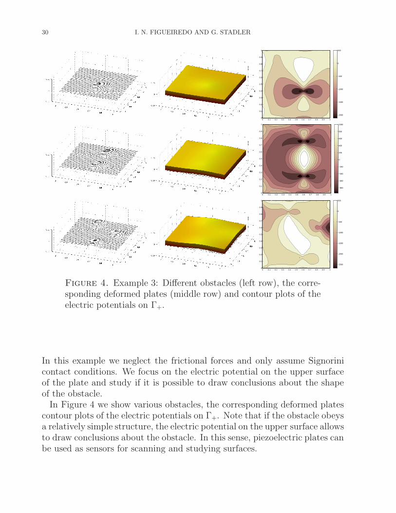
Figure 4. Example 3: Different obstacles (left row), the corre-sponding deformed plates (middle row) and contour plots of theelectric potentials on Γ+.
In this example we neglect the frictional forces and only assume Signorinicontact conditions. We focus on the electric potential on the upper surfaceof the plate and study if it is possible to draw conclusions about the shapeof the obstacle.
In Figure 4 we show various obstacles, the corresponding deformed platescontour plots of the electric potentials on Γ+. Note that if the obstacle obeysa relatively simple structure, the electric potential on the upper surface allowsto draw conclusions about the obstacle. In this sense, piezoelectric plates canbe used as sensors for scanning and studying surfaces.
FRICTIONAL CONTACT OF AN ANISOTROPIC PIEZOELECTRIC PLATE 31
Appendix. Part A. The modified tensors Aαβγρ, piαβ and pi3, in Theorem1, are defined by
Aαβγρ := Cαβγρ −Cαβ33C33γρ
C3333+
(
Cαβ33Cν333
C3333− Cαβν3
)
bδν aδγρ,
piαβ := Piαβ − Cαβ33
C3333Pi33 +
(
Pi33C33ν3
C3333− Piν3
)
bδν aδαβ ,
pi3 := εi3 +Pi33P333
C3333−
(
Pi33C33ν3
C3333− Piν3
)
bδν cδ,
where
aδγρ := C33γρCδ333 − Cδ3γρC3333, cδ := Cδ333P333 − C3333P3δ3,
[
bδν]
:=[
Cδ333C33ν3 − Cδ3ν3C3333
]−1(identity between two matrices).
We remark that p3αβ can equivalently be computed as
p3αβ := P3αβ − Cαβ33
C3333P333 +
(
Cαβ33C33ν3
C3333− Cαβν3
)
bδν cδ.
Part B. The terms (N ebciαβ (u)) and (M ebci
αβ (u)), in Theorem 2, are the com-ponents of second-order tensor fields corresponding to the Kirchhoff-Lovedisplacement u, given by the following matrix formula
[
N ebciαβ (u)
M ebciαβ (u)
]
= Oebci
[
eγρ(ζ)
∂γρζ3,
]
,
where the components of the 6 × 6 matrix Oebci are functions of the middleplane ω, namely
Oebci =
[ ∫ +h
−h Cebciαβγρdx3 −
∫ +h
−h Debciαβγρdx3
−∫ +h
−h x3Cebciαβγρdx3
∫ +h
−h x3Debciαβγρdx3
]
6×6
,

32 I. N. FIGUEIREDO AND G. STADLER
with the modified coefficients defined on Ω:
Bαβγρ := Aαβγρ +p3αβ p3γρ
p33
Cecbiαβγρ := Bαβγρ + Cecbi
αβγρ with Cecbiαβγρ =
−p3αβ aγρ
p33c0 for (ebc1),
0 for (ebc2), (ebc3),
Decbiαβγρ := x3Bαβγρ + Decbi
αβγρ with Decbiαβγρ =
−p3αβ bγρ
p33c0 for (ebc1),
0 for (ebc2), (ebc3).
The linear form lebci(.) is defined by
lebci(v) :=
∫
Ω
f · v dΩ +
∫
ΓN
g · v dΓN + lebcie (v),
with
lebcie (v) :=
∫
Ω
(
P3r + (ϕ−0 − ϕ+
0 − R) c0) p3αβ
p33eαβ(v) dx for (ebc1),
∫
Ωp3αβ
p33
(
P3r(x1, x2, x3) + (h∗θ − P3r)(x1, x2, h∗)
)
eαβ(v),
with h∗ = +1 for (ebc2) and h∗ = −1 for (ebc3).
Part C. The formulas for F ebci3 and F ebci
β , which appear in Remark 2, aredefined by
F ebci3 =
∫ +h
−h (x3∂αfα + f3) dx3 + g+3 + g−3 + h ∂α(g+
α − g−α ) + ∂αβ
(
− x3Gebciαβ
)
,
F ebciβ =
∫ +h
−h fβ dx3 + (g+β + g−β ) − ∂αG
ebciαβ for β = 1, 2,
where
Gebciαβ =
∫ +h
−h
(
P3r + (ϕ−0 − ϕ+
0 − R) c0) p3αβ
p33dx3 for (ebc1)
∫ +h
−hp3αβ
p33
(
P3r(x1, x2, x3) + (h∗θ − P3r)(x1, x2, h∗)
)
dx3,
with h∗ = +1, if i = 2 and h∗ = −1, if i = 3.
References[1] M. Bernadou and C. Haenel. Modelization and numerical approximation of piezoelectric thin
shells. I. The continuous problems. Comput. Methods Appl. Mech. Engrg., 192(37-38):4003–4043, 2003.
FRICTIONAL CONTACT OF AN ANISOTROPIC PIEZOELECTRIC PLATE 33
[2] P. Bisegna, F. Lebon, and F. Maceri. The unilateral frictional contact of a piezoelectric bodywith a rigid support. In Contact mechanics (Praia da Consolacao, 2001), volume 103 of SolidMech. Appl., pages 347–354. Kluwer Acad. Publ., Dordrecht, 2002.
[3] P. G. Ciarlet and P. Destuynder. Une justification d’un modele non lineaire en theorie desplaques. C. R. Acad. Sci. Paris Ser. A-B, 287(1):A33–A36, 1978.
[4] P. G. Ciarlet and P. Destuynder. A justification of the two-dimensional linear plate model. J.Mecanique, 18(2):315–344, 1979.
[5] Philippe G. Ciarlet. Mathematical elasticity. Vol. II, volume 27 of Studies in Mathematics andits Applications. North-Holland Publishing Co., Amsterdam, 1997. Theory of plates.
[6] Philippe G. Ciarlet. Mathematical elasticity. Vol. III, volume 29 of Studies in Mathematicsand its Applications. North-Holland Publishing Co., Amsterdam, 2000. Theory of shells.
[7] Ch. Collard and B. Miara. Two-dimensional models for geometrically nonlinear thin piezo-electric shells. Asymptot. Anal., 31(2):113–151, 2002.
[8] L. Costa, I. Figueiredo, R. Leal, P. Oliveira, and G. Stadler. Modeling and numerical study ofactuator and sensor effects for a laminated piezoelectric plate. Comput. Struct., 85(7–8):385–403, 2007.
[9] G. Duvaut and J.-L. Lions. Inequalities in mechanics and physics. Springer-Verlag, Berlin,1976. Grundlehren der Mathematischen Wissenschaften, 219.
[10] I. Ekeland and R. Temam. Convex Analysis and Variational Problems. Classics in AppliedMathematics, Vol. 28. SIAM, Philadelphia, 1999.
[11] I. Figueiredo and C. Leal. A piezoelectric anisotropic plate model. Asymptot. Anal., 44(3-4):327–346, 2005.
[12] I. Figueiredo and C. Leal. A generalized piezoelectric Bernoulli-Navier anisotropic rod model.J. Elasticity, 85(2):85–106, 2006.
[13] R. Glowinski. Numerical Methods for Nonlinear Variational Inequalities. Springer-Verlag, NewYork, 1984.
[14] J. Haslinger, M. Miettinen, and P. Panagiotopoulos. Finite element method for hemivariationalinequalities, volume 35 of Nonconvex Optimization and its Applications. Kluwer AcademicPublishers, Dordrecht, 1999.
[15] S. Hueber, A. Matei, and B. I. Wohlmuth. A mixed variational formulation and an optimala priori error estimate for a frictional contact problem in elasto-piezoelectricity. Bull. Math.Soc. Sci. Math. Roumanie (N.S.), 48(96)(2):209–232, 2005.
[16] S. Hueber, G. Stadler, and B. Wohlmuth. A primal-dual active set algorithm for three-dimensional contact problems with Coulomb friction. Technical report, Pre-publicacoes doDepartamento de Matematica da Universidade de Coimbra 06-16, 2006.
[17] T. Ikeda. Fundamentals of Piezoelectricity. Oxford University Press, 1990.[18] N. Kikuchi and J. T. Oden. Contact problems in elasticity: a study of variational inequalities
and finite element methods, volume 8 of SIAM Studies in Applied Mathematics. Society forIndustrial and Applied Mathematics (SIAM), Philadelphia, PA, 1988.
[19] S. Klinkel and W. Wagner. A geometrically non-linear piezoelectric solid shell element basedon a mixed multi-field variational formulation. Int. J. Numer. Meth. Engng, 65(3):349–382,2005.
[20] A. Leger and B. Miara. Justifying the obstacle problem in the case of a shallow shell. Technicalreport, 2006.
[21] J.-L. Lions. Perturbations singulieres dans les problemes aux limites et en controle optimal.Springer-Verlag, Berlin, 1973. Lecture Notes in Mathematics, Vol. 323.
[22] F. Maceri and P. Bisegna. The unilateral frictionless contact of a piezoelectric body with arigid support. Math. Comput. Modelling, 28(4-8):19–28, 1998.
34 I. N. FIGUEIREDO AND G. STADLER
[23] G. A. Maugin and D. Attou. An asymptotic theory of thin piezoelectric plates. Quart. J.Mech. Appl. Math., 43(3):347–362, 1990.
[24] B. Miara. Justification of the asymptotic analysis of elastic plates. I. The linear case. Asymp-totic Anal., 9(1):47–60, 1994.
[25] M. Rahmoune, A. Benjeddou, and R. Ohayon. New thin piezoelectric plate models. J. Int.Mat. Sys. Struct., 9:1017–1029, 1998.
[26] A. Raoult and A. Sene. Modelling of piezoelectric plates including magnetic effects. Asymptot.Anal., 34(1):1–40, 2003.
[27] N. Sabu. Vibrations of thin piezoelectric flexural shells: two-dimensional approximation. J.Elasticity, 68(1-3):145–165 (2003), 2002.
[28] A. Sene. Modelling of piezoelectric static thin plates. Asymptot. Anal., 25(1):1–20, 2001.[29] R. Smith. Smart material systems, volume 32 of Frontiers in Applied Mathematics. Society
for Industrial and Applied Mathematics (SIAM), Philadelphia, PA, 2005.[30] M. Sofonea and El-H. Essoufi. A piezoelectric contact problem with slip dependent coefficient
of friction. Math. Model. Anal., 9(3):229–242, 2004.[31] M. Sofonea and El-H. Essoufi. Quasistatic frictional contact of a viscoelastic piezoelectric body.
Adv. Math. Sci. Appl., 14(2):613–631, 2004.[32] L. Trabucho and J. M. Viano. Mathematical modelling of rods. In Handbook of numerical
analysis, Vol. IV, Handb. Numer. Anal., IV, pages 487–974. North-Holland, Amsterdam, 1996.[33] T. Weller and C. Licht. Analyse asymptotique de plaques minces lineairement piezoelectriques.
C. R. Math. Acad. Sci. Paris, 335(3):309–314, 2002.
Isabel N. FigueiredoCentro de Matematica da Universidade de Coimbra (CMUC), Department of Mathemat-ics, University of Coimbra, Apartado 3008, 3001-454 Coimbra, Portugal.
E-mail address : [email protected]
Georg StadlerInstitute for Computational Engineering and Sciences (ICES), The University of Texasat Austin, 1 University Station, C0200 Austin, TX 78712, USA.
E-mail address : [email protected]