NBER WORKING PAPER SERIES

FRAUDULENT INCOME OVERSTATEMENT ON MORTGAGE APPLICATIONSDURING THE CREDIT EXPANSION OF 2002 TO 2005

Atif R. MianAmir Sufi

Working Paper 20947http://www.nber.org/papers/w20947

NATIONAL BUREAU OF ECONOMIC RESEARCH1050 Massachusetts Avenue

Cambridge, MA 02138February 2015

The views expressed herein are those of the authors and do not necessarily reflect the views of theNational Bureau of Economic Research. We thank numerous colleagues from many institutions forvaluable advice and comments. We gratefully acknowledge financial support from the Fama-MillerCenter and the Initiative on Global Markets at Chicago Booth. Mian is from Princeton University andNBER: (609) 258 6718, atif@princeton.edu; Sufi is from the University of Chicago Booth Schoolor Business and NBER: (773) 702 6148, amir.sufi@chicagobooth.edu. See our websites for the appendix.

NBER working papers are circulated for discussion and comment purposes. They have not been peer-reviewed or been subject to the review by the NBER Board of Directors that accompanies officialNBER publications.

© 2015 by Atif R. Mian and Amir Sufi. All rights reserved. Short sections of text, not to exceed twoparagraphs, may be quoted without explicit permission provided that full credit, including © notice,is given to the source.

Fraudulent Income Overstatement on Mortgage Applications during the Credit Expansionof 2002 to 2005Atif R. Mian and Amir SufiNBER Working Paper No. 20947February 2015JEL No. E3,E4,E5,G01,G2,R31

ABSTRACT

Academic research, government inquiries, and press accounts show extensive mortgage fraud duringthe housing boom of the mid-2000s. We explore a particular type of mortgage fraud: the overstatementof income on mortgage applications. We define “income overstatement” in a zip code as the growthin income reported on home-purchase mortgage applications minus the average IRS-reported incomegrowth from 2002 to 2005. Income overstatement is highest in low credit score, low income zip codesthat Mian and Sufi (2009) show experience the strongest mortgage credit growth from 2002 to 2005.These same zip codes with high income overstatement are plagued with mortgage fraud accordingto independent measures. Income overstatement in a zip code is associated with poor performanceduring the mortgage credit boom, and terrible economic and financial economic outcomes after theboom including high default rates, negative income growth, and increased poverty and unemployment.From 1991 to 2007, the zip code-level correlation between IRS-reported income growth and growthin income reported on mortgage applications is always positive with one exception: the correlationgoes to zero in the non-GSE market during the 2002 to 2005 period. Income reported on mortgageapplications should not be used as true income in low credit score zip codes from 2002 to 2005.

Atif R. MianPrinceton UniversityBendheim Center For Finance26 Prospect AvenuePrinceton, NJ 08540and NBERatif@princeton.edu

Amir SufiUniversity of ChicagoBooth School of Business5807 South Woodlawn AvenueChicago, IL 60637and NBERamir.sufi@chicagobooth.edu

1

Englewood and Garfield Park are two of the poorest neighborhoods in Chicago with an

average income of $24,000 in 2000 compared to $44,000 for the rest of the city. In 1996, almost

70% of the residents in these two neighborhoods had a credit score below 660, compared to 37%

for the rest of Chicago. However, Englewood and Garfield Park experienced phenomenal growth

of 55% in mortgage credit for home purchases from 2002 to 2005, when growth was only 27%

for the rest of Chicago.

One might conclude from these facts that Englewood and Garfield Park were turning a

corner during the mortgage credit boom with higher income and economic growth. However,

income reported to the IRS from these two neighborhoods paints a different portrait. IRS-

reported annualized average income growth for these neighborhoods was only 1.9% in nominal

terms from 2002 to 2005, implying a decline in real income. Nominal income growth was 4.0%

per year for the rest of Chicago. Englewood and Garfield Park were getting poorer in both real

and relative terms, and yet mortgage credit was expanding rapidly.

We have shown in our earlier work, Mian and Sufi (2009) [MS09 henceforth], that the

“Englewood/Garfield Park” facts are not an exception, but a rule throughout the entire country.

For example, Appendix Table 1 of MS09 lists each of the top 40 MSAs by population and shows

that 39 of the 40 MSAs had slower income growth in subprime zip codes relative to prime zip

codes with an average difference of 5.1 percentage points. However, despite lower income

growth, home-purchase mortgage credit growth was faster in subprime zip codes for 33 of the 40

MSAs with an average difference of 12.6 percentage points.

In short, income growth and home-purchase mortgage origination growth were negatively

correlated in the cross-section during from 2002 to 2005. Moreover, this negative correlation was

unique to the 2002 to 2005 period. This finding, along with several others in MS09, led us to

2

conclude that the expansion of mortgage lending in neighborhoods such as Englewood and

Garfield Park during the subprime mortgage boom was driven by an expansion in credit supply

that was unrelated to improvements in borrower income.

A recent study by Adelino, Schoar, and Severino (2015) [Adelino et al, henceforth]

confirms the MS09 findings above. For example, in their summary statistics, they sort zip codes

by average 2002 IRS reported income, which we show in MS09 is strongly correlated with zip

code level credit scores. They confirm that mortgage credit expanded more in low income

neighborhoods such as Englewood and Garfield Park. They also show that these same

neighborhoods experienced lower IRS income growth from 2002 to 2005.1

However, Adelino et al dispute the use of IRS-reported income in MS09. They argue that

one should instead look at income data that is reported on mortgage applications of home buyers.

They use income reported on mortgage applications to argue that the income growth of home

buyers was increasing in neighborhoods experiencing higher mortgage credit growth. So while

the overall income growth of the neighborhoods such as Englewood and Garfield Park was

declining, Adelino et al argue, the buyers themselves had strong positive income growth. Based

on this finding, they argue there was no change in the lending technology during the mid-2000s.

So how does this argument apply to Englewood and Garfield Park? The annualized

growth in income reported on mortgage applications for home purchase was 7.7%. This is very

high—the average growth in income reported on mortgage applications for the rest of Chicago

was 4.3%. The gap between the growth in income reported on mortgage applications of home

1 Adelino et al do not comment on our research showing how home-equity based borrowing contributed to the aggregate rise in the household debt to income ratio (Mian and Sufi (2011), Mian and Sufi (2014a)). They also do not comment on our research on the importance of household debt in the Great Recession (Mian and Sufi (2010, 2014b, 2014c), Mian, Rao, and Sufi (2013)).

3

buyers and IRS reported income growth in Englewood and Garfield Park was 5.8 percentage

points, compared to almost no gap in other Chicago neighborhoods.

In Chicago, the reasoning of Adelino et al would imply that the gap between the growth

in income reported on mortgage applications and IRS income growth reflects individuals with

exceptionally high income buying homes in Englewood and Garfield Park. Anyone who knows

Chicago would be skeptical of this reasoning. Englewood and Garfield Park were very poor in

2000, saw incomes decline from 2002 to 2005, and they remain very poor neighborhoods today.

In fact, median household income in 2010 fell in nominal terms from 2000 to 2010, implying

substantially negative real income growth. In 2012, the two neighborhoods had the highest rate

of violent crime per resident in Chicago. These facts are hard to reconcile with the notion that

individuals with high income were buying homes from 2002 to 2005.

The far more likely explanation for the pattern unveiled by Adelino et al is fraudulent

income overstatement on mortgage applications, and indeed 3 of the 4 zip codes that make up

Englewood and Garfield Park eventually were on a list of top mortgage fraud zip codes put

together by the mortgage fraud detection company InterThinx.

In this study, we take a systematic look at fraudulent overstatement of income on

mortgage applications during the 2002 to 2005 period. We focus on the difference between the

annual growth in income reported on mortgage applications between 2002 and 2005 (the

measure used by Adelino et al) and the annual growth in IRS reported income between 2002 and

2005 (the measure used by MS09). We refer to this difference as “buyer income overstatement,”

and we construct this variable at the zip code level.

Zip codes with high buyer income overstatement during the boom had lower credit

scores, lower income, higher poverty rates, higher unemployment, and lower education levels

4

before the boom. Englewood and Garfield Park exemplify the broader pattern across the United

States. These correlations are crucial to understanding the Adelino et al results. In essence, their

argument is that the same subprime zip codes analyzed in MS09 were seeing high income

individuals buying homes—buying homes in traditionally poor, low credit score neighborhoods.

Instead, we demonstrate that buyer income overstatement was higher in low credit score

zip codes because of fraudulent misreporting of buyers’ true income. We do so in three ways.

First, we show that well-known and proven incidents of mortgage fraud were much

higher in zip codes with high buyer income overstatement. In particular, zip codes with high

buyer income overstatement witness a larger increase in the fraction of non-agency mortgages,

and in particular mortgages with low or unknown documentation. We know from a large body of

research that both non-agency securitized mortgages and low-doc mortgages were associated

with a high incidence of fraud (e.g., Ben-David (2011); Jiang, Nelson, and Vytlacil (2014),

Griffin and Maturana (2014); Piskorski, Seru, and Witkin (2015)).

Moreover, using data compiled by Piskorski, Seru, and Witkin (2015), we show that

mortgages made in high buyer income overstatement zip codes were significantly more likely to

be fraudulently reported as being for an owner-occupied property, or had deliberately omitted

information on second liens. Using a list of zip codes with the highest amount of mortgage fraud

according to InterThinx, we show that this independent measure of fraud is also strongly

positively correlated with buyer income overstatement from 2002 to 2005.

Second, contrary to the hypothesis that buyer income overstatement represents

“gentrification” of these zip codes, we show that buyer income overstatement forecasts negative

income and financial outcomes. In every year of the mortgage credit boom, we calculate the

difference between the average income reported on mortgage applications in a zip code and the

5

IRS average income of all residents living in a zip code. We then show that zip codes with a

large positive difference between buyer income from mortgage applications and IRS average

income experienced subsequently lower IRS income growth in the following year. Further,

according to IRS data, high borrower income overstatement zip codes saw a relative decline in

the number of high income individuals living in the zip code. We also use individual level data

on credit scores to show that people moving into high borrower income overstatement zip codes

do not have better credit scores than residents already living there.

Looking past 2005, we find that zip codes with high overstatement perform terribly.

Default rates in these zip codes skyrocketed from 2005 to 2007. Using a longer horizon, the zip

codes with high overstatement from 2002 to 2005 experienced lower IRS income and wage

growth from 2005 to 2012. They also saw lower median household income growth from 2000 to

2010 according to the Census. Finally, there was a jump in both poverty and unemployment rates

from 2000 to 2010. Recall, these zip codes already had higher poverty and unemployment rates

in 2000, and they increased further through 2010. These patterns are inconsistent with

gentrification, but consistent with fraudulent income overstatement on mortgage applications.

Third, time-series evidence on buyer income overstatement over a longer horizon shows

that income reported on mortgage applications was particularly distorted during the 2002 to 2005

period. The correlation between buyer income growth and IRS-reported income growth across

zip codes is weakest during the 2002 to 2005 period relative to earlier and subsequent periods.

Moreover, the weak correlation during the 2002 to 2005 period is driven entirely by zip codes

with a high share of non-GSE mortgage originations. There was a decoupling of buyer income

growth and IRS income growth concentrated exactly when we believe fraud was most prevalent:

among mortgages originated from 2002 to 2005 sold for non-GSE securitization.

6

We should note that for comparison to our earlier work, we use exactly the same sample

that was used in MS09. We added a few variables to this sample which we describe later.

However, we also show robustness of our main results to the full sample of zip codes beyond the

original MS09 sample. For more information on the underlying data, please see MS09 and the

online appendix associated with it.

I. Buyer Income Overstatement

A. Core Issue

In MS09, we attempted to explain why the expansion in mortgage credit for home

purchase and subsequent default crisis was more dramatic in zip codes where residents had low

credit scores, which we referred to as “subprime zip codes.” We concluded that the expansion of

mortgage credit for home purchase to subprime zip codes was driven by a credit supply shift that

was unrelated to improvements in income growth of borrowers. To support this claim, we

showed that subprime zip codes experienced a decline in income from 2002 to 2005. We also

showed that the expansion of mortgage credit to subprime zip codes with falling income induced

a negative correlation between mortgage credit growth and income growth at the zip code level.

The correlation between credit growth and income growth was positive in all other periods.

Formally, we estimated coefficients for the following specification:

𝑀𝑀𝑀𝑀𝑀𝑀𝑀𝑀𝑀𝑀𝑀𝑀𝑀𝑀𝑀𝑀𝑀𝑀𝑀ℎ𝑐𝑐𝑐 = 𝛼𝑐 + 𝛽𝑐 ∗ 𝐼𝐼𝐼𝐼𝐼𝐼𝑀𝐼𝑀𝑀𝑀𝑀𝑀𝑀ℎ𝑐𝑐𝑐 + 𝜀𝑐𝑐𝑐 (1)

where 𝛼𝑐 are county fixed effects, 𝑀𝑀𝑀𝑀𝑀𝑀𝑀𝑀𝑀𝑀𝑀𝑀𝑀𝑀𝑀𝑀𝑀𝑀𝑀ℎ𝑐𝑐𝑐 is the growth in total amount of

mortgage credit originated for home purchase in zip code z in county c during time period t. The

key specification focused on growth from 2002 to 2005. As a result, our coefficient estimate of 𝛽

7

reflected the cross-sectional correlation between IRS income growth and the growth in total

mortgage originations for home purchase across zip codes from 2002 to 2005.

Column 1 of Table 1 reports the coefficient estimate of 𝛽 that we found in MS09. As we

have already mentioned, we found a strong negative correlation between mortgage credit growth

and IRS income growth across zip codes from 2002 to 2005, but a positive correlation in all

other time periods. Two points to note about the specification. First, we advocated the use of

county fixed effects. The full justification for the use of county fixed effects is given in detail in

MS09 (in the introduction), and we refer the reader to that paper for details. Second, the sample

used in MS09 was limited to the zip codes for which we had house price data at the time (the

Fiserv Case Shiller Weiss index to be precise). In the interest of comparability, we will continue

to use the MS09 sample in this paper. However, we show the robustness of all our key results in

the full sample toward the end.

As mentioned in the introduction, Adelino et al confirm these results. However, they

prefer estimation of equation (1) with income information of home buyers reported on mortgage

applications. They argue that zip level IRS income does not necessarily represent the income

profile of the actual buyers purchasing a home in a given zip code during the mortgage credit

expansion. Notice that if there were only a fixed time-invariant difference between mortgage

application income and IRS average income at the zip code level, it would be eliminated by our

first difference specification. So Adelino et al have a more specific critique in mind: namely,

from 2002 to 2005, the selection of buyers was systematically different in zip codes experiencing

the most rapid mortgage credit growth. The argument they give is that higher income growth

buyers were systematically buying homes in areas that otherwise had slow or even negative real

IRS income growth.

8

Motivated by this reasoning, Adelino et al estimate the following specification:

𝑀𝑀𝑀𝑀𝑀𝑀𝑀𝑀𝑀𝑀𝑀𝑀𝑀𝑀𝑀𝑀𝑀𝑀𝑀ℎ𝑐𝑐𝑐 = 𝛼𝑐 + 𝛾𝑐 ∗ 𝐵𝐵𝐵𝑀𝑀𝐼𝐼𝐼𝑀𝐼𝑀𝑀𝑀𝑀𝑀𝑀ℎ𝑐𝑐𝑐 + 𝜀𝑐𝑐𝑐 (2)

where 𝐵𝐵𝐵𝑀𝑀𝐼𝐼𝐼𝑀𝐼𝑀𝑀𝑀𝑀𝑀𝑀ℎ𝑐𝑐𝑐 is the growth in income reported on mortgage applications for

individuals buying homes in zip code z in county c in period t. In column 2 of Table 1, we

estimate equation (2) in our sample for the 2002 to 2005 period, and we confirm their finding:

buyer income growth according to mortgage applications is positively correlated with mortgage

credit growth from 2002 to 2005. In column 3 we put in both IRS income growth and buyer

income growth, and the coefficient estimates on both remain statistically significant and almost

unchanged. The fact that both estimates are almost identical reflects the fact that buyer income

growth and IRS income growth in a zip code are only weakly correlated from 2002 to 2005, a

fact we will show is unique to this time period.

In column 4 of Table 1, we construct a key variable we will use throughout this study:

buyer income overstatement. It is defined to be the difference between the two income growth

measures used in column 3. More specifically:

𝐵𝐵𝐵𝑀𝑀𝐼𝐼𝐼𝑀𝐼𝑀𝐵𝐵𝑀𝑀𝐵𝑀𝑀𝑀𝑀𝐼𝑀𝐼𝑀𝑐𝑐,02−05

= 𝐵𝐵𝐵𝑀𝑀𝐼𝐼𝐼𝑀𝐼𝑀𝑀𝑀𝑀𝑀𝑀ℎ𝑐𝑐,02−05 − 𝐼𝐼𝐼𝐼𝐼𝐼𝑀𝐼𝑀𝑀𝑀𝑀𝑀𝑀ℎ𝑐𝑐,02−05

In words, buyer income overstatement is the difference in the annualized growth in income on

mortgage applications of home buyers and annualized IRS income growth of residents in a zip

code. The mean of buyer income overstatement from 2002 to 2005 is 1.7 percentage points. On

average across zip codes from 2002 to 2005, income reported on mortgage applications of home

buyers grew by 1.7 percentage points (annualized) more than IRS income growth of residents

living in the zip code. But there is wide variation: at the 90th percentile of the distribution, buyer

income overstatement is 11 percentage points.

9

Another way of phrasing the Adelino et al result is that home purchase credit growth

from 2002 to 2005 is stronger in zip codes where income growth of home buyers on mortgage

applications was higher than IRS reported income growth for the zip code as a whole. We show

this result in column 4: buyer income overstatement strongly predicts mortgage credit growth

from 2002 to 2005.2

The key question is: Why is buyer income overstatement positively related to mortgage

credit growth from 2002 to 2005? Adelino et al assert that it is because higher income

individuals were buying homes in otherwise low income growth zip codes, and this was

especially true in zip codes with high mortgage credit growth. We argue in the rest of this study

that buyer income overstatement reflects fraudulent income reporting on mortgage applications,

and such fraudulent income reporting was more prominent in the same subprime zip codes MS09

show were experiencing high mortgage credit growth from 2002 to 2005.

B. Core Issue, Visually

Figure I helps reveal visually what is going on with buyer income overstatement during

the mortgage credit boom. We first calculate the ratio of income of home buyers reported on

mortgage applications to average IRS income in a zip code. A higher ratio implies that that the

income of home-buyers reported in mortgage applications is higher than average incomes in the

zip code. We then plot this ratio across the zip-code level IRS average income distribution, and

we separately plot this for 1998, 2001, 2005, and 2011.

One can see how unusual the mortgage credit boom was. In 2005, the ratio of buyer

income from mortgage applications to IRS income is higher than it was during previous years

2 Given that buyer income overstatement is buyer income growth minus IRS income growth, column 4 is a constrained version of column 3 where we impose that the coefficients are the same on the two income growth measures but with opposite sign. We could also define borrower income overstatement as 0.43*buyer income growth minus 0.71*IRS income growth to be consistent with column 3. For the ease of interpretation, we use the raw difference as buyer income overstatement, but all results are similar if we used this alternative definition.

10

across almost the entire distribution. So in the aggregate, income reported on mortgage

applications relative to IRS income was exceptionally high in 2005, which would imply in the

aggregate that high income individuals were marginal buyers of homes during the mortgage

credit boom. This is inconsistent with the large body of research that credit expanded to low

credit score, low income individuals during the boom. In the Survey of Consumer Finances, for

example, the average income of homeowners fell in real terms from 2001 to 2004 from $114

thousand to $107 thousand (in 2013 dollars).

Further, mortgage application income in 2005 is especially high at the low end of the

income distribution. The jump in the ratio at the 1st and 2nd decile of the income distribution is

exceptionally large: In 2005, buyer income was 2.5 to 3 times higher than the average income of

residents. The ratio was between 1.5 and 2 in prior years. Equally striking is the fact that while

the ratio of mortgage application to IRS-reported income jumps for low income zip codes in

2005 relative to 2001, the jump is not sustained in subsequent years. Figure I shows that by 2011,

the pattern between the income multiple and income decile of zip codes reverts back to its

historical trend. The mortgage credit boom is anomalous.

The black arrow in Figure I isolates the core issue at hand. Adelino et al assert that the

tremendous jump in the ratio of mortgage application income to average IRS income in poor

areas in 2005 was due to high income individuals buying homes in poor areas. An alternative

interpretation is that the jump is driven by fraudulent reporting of income that especially plagued

low income, high subprime neighborhoods. We will return to the fraud evidence in Section II.

But we first present descriptive characteristics of the zip codes that had high buyer income

overstatement during the 2002 to 2005 period.

C. Characteristics of High Buyer Income Overstatement Zip Codes

11

Table 2 presents within-county correlations between buyer income overstatement from

2002 to 2005 and zip-level characteristics. Zip codes with high buyer income overstatement have

a higher fraction of subprime borrowers, lower income, higher poverty, lower education, higher

unemployment, and higher defaults in 2000. The correlations have small standard errors, with t-

statistics in from 8 to 10. Table 2 shows that the zip codes with high buyer income overstatement

from 2002 to 2005 are the same subprime zip codes MS09 show experienced tremendous

mortgage credit growth during the boom. We should therefore not be surprised that high buyer

income overstatement predicts higher mortgage credit growth.

Figure II plots buyer income overstatement from 2002 to 2005 across the distribution of

1996 credit scores (left) and 2002 IRS average income (right). This is a raw plot of the data –

there are no county fixed effects. As it shows, subprime and low income zip codes have much

higher buyer income overstatement. The lowest credit quality zip codes have buyer income

overstatement of 6 percentage points: that is, from 2002 to 2005, income of buyers according to

mortgage applications in low credit score zip codes increased by 6 percent (annualized) more

than IRS income. Recall from the introduction that buyer income overstatement was about 6

percentage points in Englewood and Garfield Park.

Buyer income overstatement during the mortgage credit boom was highest in low credit

score, poor zip codes. This is exactly what we would expect if it was due to mortgage fraud.

Suppose a mortgage originator and potential home buyer 𝑧 with true income 𝐼𝑐 want to close a

mortgage for home purchase. The originator and applicant may work together to falsify the

applicant’s income 𝐼𝑐 ≠ 𝐼𝑐 depending on the size of the mortgage relative to his income

potential, and the likelihood that they can get away with misreporting income. If the potential

buyer has more than sufficient income to get the loan, then he is not credit-constrained at the

12

margin. In such a situation, there is no incentive to misreport. However, if the potential buyer

does not have sufficient income to get the mortgage, then the originator and buyer may have an

incentive to over-report income 𝐼𝑐 > 𝐼𝑐. Such overstatement is likely to take place in zip codes

where incomes and credit scores are low.

Notice in this example that the mortgage originator and buyer work together to commit

fraud. Normally, it would be the duty of the mortgage originator to help stem misreporting.

However, during the mortgage credit expansion from 2002 to 2005, we know originators failed

to monitor and screen potential borrowers (e.g., Keys, et al (2010)). In fact, there are numerous

examples where mortgage brokers or originators may have falsified income information by

borrowers without the borrowers’ knowledge.3 We will see some of these examples below.

II. Mortgage Fraud in Zip Codes with High Buyer Income Overstatement

A. Existing Research

The use of self-reported information on mortgage applications as true income must be

viewed within the context of extensive research documenting serious fraud in the mortgage

market during the early to mid-2000s. Fraud, by its nature, is difficult to detect; as a result,

aggregate definitive estimates of fraud are difficult to obtain. But we know fraud was

widespread.

For example, as the Financial Crisis Inquiry Commission reports, “Ann Fulmer, vice

president of business relations at Interthinx, a fraud detection service, told the FCIC … that

about $1 trillion of the loans made during the [2005 to 2007] period were fraudulent” (FCIS,

Chapter 9, 2011). The FCIC dedicated an entire section of their report – 14 pages – on the 3 See for example the series of award winning articles by Binyamin Appelbaum on mortgage fraud in Charlotte in the Charlotte Observer: http://www.charlotteobserver.com/2009/06/04/762690/sold-a-nightmare-part-1-of-4.html#.VMvJXmjF9g0

13

prevalence of mortgage fraud during the housing boom. Zingales (2015) reports that $113B of

fines have been levied against lenders based on mortgage fraud during the housing boom, and he

further emphasizes that this number “severely underestimates the magnitude of the problem.”

On the specific issue of income overstatement, an article by Matt Taibbi cites an

employee at JPMorganChase who discovered that “around 40 percent of [mortgages] were based

on overstated incomes.”4 A complaint against CountryWide filed in Illinois reports that “the

Mortgage Asset Research Institute reviewed 100 stated income loans, comparing the income on

the loan documents with the borrowers’ tax documents. The review found that almost 60% of the

income amounts were inflated by more than 50% …”5 The Federal Reserve Board assessed an

$85 million civil money penalty against Wells Fargo because employees “… separately falsified

income information in mortgage applications.”6 According to an article in the Los Angeles

Times, employees at mortgage lender Ameriquest testified that they had witnessed behavior

including “deceiving borrowers about the terms of their loans, forging documents, falsifying

appraisals and fabricating borrowers’ income to qualify them for loans they couldn’t afford.”7 As

Michael Hudson, a Wall Street Journal reporter, writes in his book:

At the downtown L.A. branch [of mortgage lender Ameriquest], some of Glover's coworkers had a flair for creative documentation. They used scissors, tape, Wite-Out, and a photocopier to fabricate W-2s, the tax forms that indicate how much a wage earner makes each year. It was easy: Paste the name of a low-earning borrower onto a W-2 belonging to a higher-earning borrower and, like magic, a bad loan prospect suddenly looked much better. Workers in the branch equipped the office's break room with all the tools they needed to manufacture and manipulate official documents. They dubbed it the ‘Art Department.’8

4 Taibbi, Matt, 2014, “The $9 Billion Witness: Meet JPMorgan Chase’s Worst Nightmare,” Rolling Stone Nov 6th. 5 The filing is available at: http://www.illinoisattorneygeneral.gov/pressroom/2008_06/countrywide_complaint.pdf 6 Federal Reserve Board Press Release, July 20, 2011, available at: http://www.federalreserve.gov/newsevents/press/enforcement/20110720a.htm 7 Hudson, Mike and E. Scott Reckard, 2005. “Workers Say Lender Ran “Boiler Rooms,” Los Angeles Times, February 4th. 8 The Monster: How a Gang of Predatory Lenders and Wall Street Bankers Fleeced America—and Spawned a Global Crisis, St. Martin’s Griffin, 2011.

14

These articles generally focus on mortgages provided for low income, low credit score

individuals.9

Academic research supports the argument that fraud was endemic to mortgage markets

during this period. Griffin and Maturana (2014) examine securitized non-agency loans and find

that 30% of loans exhibited some kind of misrepresentation. Misrepresentation was widespread

in both low and full documentation loans within the non-agency market. Piskorski, Seru, and

Witkin (2015) also examine the non-agency mortgage market and find 1 out of 10 had

misrepresentation. Both of these studies focus on misrepresentation where MBS buyers were

misled on characteristics of the mortgage related to owner-occupied status, the presence of

second lien, and over-stated property value appraisals. Ben-David (2011) focuses on inflated

appraisals in Chicago and finds that 16% of highly leveraged transactions had inflated prices.

The most relevant study for buyer income overstatement is Jiang, Nelson, and Vytlacil

(2014). Their research design focuses on mortgages originated by a single bank from 2004 to

2008, and they have the advantage of seeing all information collected by the bank in addition to

ex post default on the mortgages. To detect income exaggeration, they treat the full

documentation loans in their sample as the control group, and they see how reported information

on low documentation loans compares to the income information on full documentation loans.

They conclude through their analysis that low documentation mortgage applications inflated

incomes by an average of 28.7% relative to high documentation mortgages.

Jiang, et al (2014) also make clear that their results should be viewed as a lower bound

given the strategy. It assumes honest reporting on full documentation loans in the non-agency

market, and it is limited by the inability to see true income of the low documentation buyers. As

they note: “As these are conservative estimates, the data suggest serious income falsification 9 We are grateful to Binyamin Appelbaum of the New York Times for providing us with many of these cites.

15

among low-documentation borrowers using full-documentation borrowers as a benchmark” (our

emphasis). Recall from the studies above that evidence of other types of fraud has been detected

in full documentation loans as well.

What are the important lessons from the existing research? First, fraud was endemic to

mortgage markets during the mortgage credit boom and income on mortgage applications was

routinely falsified. Second, the estimates of fraud from this literature are by their nature lower

bound estimates. The researchers in these studies have made a conscious effort to only report

fraud when they can explicitly detect it. For example, Griffin and Maturana (2014) write: “This

suggests that our misrepresentation indicators may not be capturing the full extent of

misrepresented loans or some other aspect of poorly performing originating practices that are

correlated with mortgage misrepresentation.” Dyck, Morse, and Zingales (2014) make an

important point in the context of corporate fraud: detected frauds are only the tip of the iceberg

in terms of actual fraud occurring. Third, fraud has been proven to be widespread in the non-

agency mortgage market, which offers useful guidance for where mortgage applications were

most likely to fraudulently overstate income.

B. Measuring Fraud Directly

Table 3 shows evidence that mortgage fraud was more prevalent in zip codes with high

borrower income overstatement. In columns 1 and 2, we show that zip codes with high

overstatement saw a larger increase in the share of mortgages originated for non-agency

securitization.10 This is almost completely driven by an increase in the share of low

documentation mortgages originated for non-agency securitization. We know from research cited

above that low-documentation non-agency securitization experienced rampant mortgage fraud

from 2002 to 2005, and in particular fraudulent overstatement of income. 10 Data on non-agency and low documentation mortgages are from BlackBox Logic.

16

In columns 3 and 4 of Table 3, we use information from InterThinx, a mortgage fraud

detection company. Since the second quarter of 2010, they have released a list of the zip codes

with the most rampant mortgage fraud. More specifically, they focus on four types of fraud:

property valuation, identity, occupancy, and employment/income. The top mortgage fraud zip

codes are inclusive of all of these types of fraud. They reveal a top 10 list every quarter, and then

an annual list every year of 20 or 25 zip codes. An obvious drawback is that they began releasing

the list in 2010, well after the mortgage credit boom. However, there is strong persistence

between 2010 and 2014 of the zip codes that make the list, which suggests that mortgage fraud is

a fixed characteristic of zip codes that can be used retrospectively to examine fraud during the

subprime mortgage credit boom. Column 3 shows that zip codes with high buyer income

overstatement from 2002 to 2005 are more likely to make the InterThinx top fraud list in 2010,

and column 4 shows that they are more likely to make the InterThinx top fraud list at some point

between 2010 and 2014.

Figure III utilizes the InterThinx data to show how high buyer income overstatement is in

zip codes that make the top fraud list. In the 18 zip codes that made the top fraud list at some

point in 2010, buyer income overstatement from 2002 to 2005 was more than 10 percentage

points, compared to an average of about 2 percentage points for the rest of the sample.

In columns 5 through 7, we use data from the study by Piskorski, Seru, and Witkins

(2015). They study two types of fraud in the non-agency market from 2005 to 2007: misreporting

of the owner-occupant status of a property and misreporting of whether a second-lien is present.

This is a different type of fraud than fraudulent income overstatement. Nonetheless, we continue

under the assumption that zip codes with fraud on these measurable dimensions also had fraud in

income reported on mortgage applications during the mortgage credit boom.

17

The exact left hand side variable we use is the fraction of non-agency securitized

mortgages in a zip code where Piskorski, Seru, and Witkins (2015) detect fraud on the

dimensions discussed above.11 As columns 5 through 7 of Table 3 show, there is a strong

correlation between buyer income overstatement in a zip code and these alternative measures of

fraud. The statistical significance is high, with t-statistics on the order of 7 to 10. In summary,

columns 3 through 7 show that mortgage fraud was more likely in the zip codes where mortgage

applications were reporting higher buyer income than local resident income.

III. Do High Buyer Income Overstatement Zip Codes Improve?

As mentioned before, fraud, by its nature, is difficult to detect. We present evidence in

the previous section that fraud was indeed rampant in the zip codes where mortgage applications

significantly overstated income growth. In this section, we take a different approach. If high

income growth individuals were buying homes in low income growth zip codes, we should

eventually see some evidence of improvement. In this section, we present evidence of the

opposite. Zip codes with high borrower income overstatement were already poor before 2002,

and their incomes fell even further both during and after the mortgage credit boom.

A. Contemporaneous Performance

In Table 4, we estimate the following cross-sectional regression for each period t-1 to t:

ln(𝐼𝐼𝐼𝐼𝐼𝐼𝑐𝑐𝑐) − ln�𝐼𝐼𝐼𝐼𝐼𝐼𝑐𝑐,𝑐−1� = 𝛼𝑐 + [ln�𝐵𝐵𝐵𝑀𝑀𝑐𝑐,𝑐−1� − ln (𝐼𝐼𝐼𝐼𝐼𝐼𝑐𝑐,𝑐−1)] ∗ 𝛾𝑐 + 𝜀𝑐𝑐

In words, this specification tests whether IRS income grows faster between t-1 and t in zip codes

where at t-1 buyer income is higher than IRS income. This is a simple test for gentrification:

does the presence of home buyers with higher than average income in the zip code predict future

11 We are thankful to Amit Seru for providing us with these data.

18

IRS income growth in the zip code? Zip level IRS income data are available for 1991, 1998,

2002, 2004, 2005, and 2006, which means we run five cross-sectional regressions using the

periods 1991 to 1998, 1998 to 2002, 2002 to 2004, 2004 to 2005, and 2005 to 2006.

Prior to the mortgage credit boom, we find positive estimates for 𝛾: of a positive

difference between income on mortgage applications and average IRS income predicts higher

IRS growth. But from 2002 to 2005, the relationship reverses. During the boom, a positive

difference between buyer and IRS income at time t predicts a decline in IRS income growth from

t to t+1. Zip codes with high buyer income growth relative to IRS income growth experienced

subsequently worse economic performance during the mortgage credit boom, not better. This is

consistent with mortgage fraud during the boom, and inconsistent with gentrification.

In column 6, we regress the change in the fraction of IRS returns in the zip code that have

greater than $50 thousand in adjusted gross income. High buyer income overstatement zip codes

experience a relative decline in IRS returns with high incomes during the boom. Column 7 uses

credit score of individuals in the data used in Mian and Sufi (2011). We measure the credit score

of people moving into a zip code from 2002 to 2005 minus the credit scores of people living in

the zip code as of 2002 according to the credit bureau. The point estimate suggests that high

buyer income overstatement zip codes saw a relative decline in the credit scores of individuals

moving in versus those living in the zip code, contradicting the argument that these zip codes

were gentrifying. Recall that high buyer income overstatement zip codes have lower credit scores

in 2002, and those moving in during the 2002 to 2005 boom did not have higher scores.

B. Future Performance

In Table 5, we take a longer view by regressing measures of future performance on buyer

income overstatement from 2002 to 2005. Zip codes with high buyer income overstatement saw

19

lower IRS income and wage growth from 2005 to 2012, a decline in Census income growth from

2000 to 2010, and an increase in both poverty rates and unemployment rates from 2000 to

2010.12 The census result and the wage growth result is important because average IRS income

can be distorted by the number of individuals filing in a given year, and the decision of high net

worth individuals to exercise capital gains. The poverty result is especially revealing. Poverty

rates in 2000 were already significantly higher in zip codes with high buyer income

overstatement from 2002 to 2005 (Table 2). And yet they jumped even higher from 2000 to

2010. As columns 6 and 7 show, the default rate also jumped substantially higher in zip codes

with high buyer income overstatement. This latter result is consistent with Jiang, et al (2014)

who find that fraudulent income overstatement on mortgage applications predicts default.

Figure IV shows real income growth from 2005 to 2012 by buyer income overstatement

during the boom. We plot income growth according to three measures: IRS income growth,

income reported on mortgage applications for home purchase, and income reported on mortgage

applications for refinancing.13 According to all three measures, there was an absolute decline in

real income in zip codes with high borrower income overstatement during the boom. The decline

is 40% for home purchase applications in high buyer income overstatement zip codes. This

reflects how unusually high the income reported on mortgage applications was in 2005.

The results in Tables 4 and 5 and Figure IV cast doubt on the interpretation that high

income growth reported on mortgage applications in high mortgage credit growth zip codes

reflects an influx of higher income households to these neighborhoods during the boom. If high

income growth individuals were buying homes in lower credit score poorer zip codes, we should

eventually see some evidence of improved economic circumstances. We do not see any such

12 The 2010 data on median household income, poverty, and unemployment rate come from the 2008-2012 vintage of the American Community Survey, which replaces the 2010 decennial Census. 13 We do not have the 2012 HMDA data yet, which is why the HMDA measures only go through 2011.

20

evidence. In fact, we see the opposite. The results are more consistent with fraudulent income

overstatement on mortgage applications in low income neighborhoods from 2002 to 2005.

IV. The Decoupling of Self-Reported and IRS-Reported Income

How unusual is it that income growth of home buyers reported on mortgage applications

deviates strongly from IRS-reported income growth of a zip code? Table 6 regresses the growth

in income reported on mortgage applications of home buyers in a zip code on IRS-reported

income growth of the zip code over various time periods between 1991 and 2007.

We find a significant reduction in the correlation between mortgage-application reported

income growth of home buyers and IRS income growth from 2002 to 2005. In fact, we can easily

reject the hypothesis that the coefficient estimate from 2002 to 2005 is the same as it was before

the mortgage credit boom. The correlation between buyer income growth and IRS income

growth breaks down significantly during the credit boom period.

Why does the correlation between buyer income growth and IRS income growth break

down during from 2002 to 2005? Research cited above suggests that fraudulent overstatement of

income was common among mortgages sold into the non-GSE securitization market. Table 7

investigates this by estimating this correlation separately for the four quartiles of zip codes by

GSE share during 2002 to 2005.14 We classify zip codes into the four quartiles according to the

average share of mortgages sold to GSEs for securitization from 2002 to 2005. We keep zip

codes in the same category for all time periods.

The results show that the breakdown in the correlation between buyer income growth and

IRS income growth during 2002 to 2005 is entirely driven by zip codes with a low share of non-

GSE mortgages. There is no change in the correlation between buyer income growth and IRS 14 Sorting by 1996 zip code level credit scores instead of GSE share leads to qualitatively similar results.

21

income growth in the zip codes with a high share of GSE mortgages. Further, the correlation

between the growth in buyer income on mortgage applications and IRS income growth is

positive in high non-GSE mortgages outside the 2002 to 2005 period. The decoupling is

concentrated when and where fraud was most likely: high non-GSE share zip codes during the

mortgage credit boom.

The results in Table 7 support the view that income reported on mortgage applications in

the GSE market reflected fundamental income during 2002 to 2005, whereas income reported on

mortgage applications in the non-GSE market were fraudulently overstated. This is consistent

with evidence we have already seen: buyer income overstatement was higher in subprime zip

codes (Figure I, Figure II, Table 2). Moreover, the share of non-agency mortgages increased the

most in zip codes with high buyer income overstatement (Table 3).15

V. Specific Comments on Adelino et al Tests

Adelino et al make some specific arguments to suggest that correlation between mortgage

origination growth and income growth remained positive during 2002 and 2005, and that

fraudulent income reporting is not a major concern in their study. We discuss these arguments

separately below.

A. Correlation between Average Mortgage Size and IRS-reported Income Growth

MS09 show that the growth in the total amount of mortgage originations as well as

growth in the total number of mortgages issued is stronger in zip codes with declining IRS

income growth during 2002 to 2005. We argued that this result reflects a shift in the supply of

15 This supports the argument in Keys, Seru, and Vig (2011) who note: “our results suggest that the policy debate regarding securitization and lenders’ underwriting standards should separately evaluate the agency and non-agency markets …”.

22

credit that other tests in MS09 verify. Adelino et al confirm the MS09 results using both growth

in mortgage amount and the growth in number of originations as the dependent variable.

However, Adelino et al also use the growth in average mortgage size conditional on

origination as the dependent variable and show that the growth in average mortgage size is

positively correlated with IRS income growth. In other words, they run the regression in column

(1) of our Table 1, but with growth in average mortgage size conditional on origination as the

dependent variable. We also confirm the Adelino et al result in our sample.

Adelino et al assert that this positive correlation contradicts the MS09 view that mortgage

origination growth among subprime zip codes was driven by an outward shift in credit supply.

We disagree. In fact, a logical conclusion of the MS09 credit supply hypothesis is precisely that

one would observe a negative correlation between growth in total mortgage origination and

growth in income, but a positive correlation between growth in average mortgage size and

growth in income.

The basic point is that marginal loans being issued in high credit growth areas are likely

to be smaller in size. Keep in mind the basic facts from MS09: credit growth is fastest in

subprime zip codes that are poorer zip codes with cheaper houses. Moreover, IRS income growth

is also lower in these zip codes. Therefore faster credit growth in these zip codes will tend to

reduce the average mortgage size, creating a positive correlation between growth in average

mortgage size and growth in IRS income.

Here is a simple numerical example to illustrate this point. Suppose in 2002 we have two

zip codes, high credit score and low credit score. Within the high credit score zip code, there are

two prime borrowers, both of which get a mortgage of 100 to buy a home in 2002. Within the

low credit score zip code, there is a prime borrower and a subprime borrower. The prime

23

borrower also gets a mortgage of 100 to buy a home, but the subprime borrower cannot get a

mortgage because he is rationed out of the market. Now fast forward to 2005, and let’s suppose

that lenders become willing to lend to the subprime borrower (a credit supply shift), but only at a

lower amount of 50 (which the lender wasn’t willing to lend in 2002). Let us also assume that the

three prime borrowers buy a new home with the exact same mortgage of 100 in 2005.

What will we find in the data for this example? Total mortgage origination growth from

2002 to 2005 is 0% in the high credit score zip code, and 50% in the low credit score zip code

(from 100 to 150). This is the MS09 result. But what about the growth in average mortgage size?

Average mortgage size does not change in the high credit score zip code (100 before and 100

after), but it declines in the low credit score zip code (100 before and 75 after). We already know

from MS09 that IRS income growth from 2002 to 2005 is stronger in high credit score zip codes.

This example yields exactly the Adelino et al result: average mortgage size will be positively

correlated with IRS income growth.

The example constructed above is based on the MS09 credit supply hypothesis. The

correlation between total origination growth and income growth is negative, while the correlation

between growth in average mortgage size and income growth is positive. In short, a positive

correlation between growth in average mortgage size and income growth is perfectly consistent

the conclusions in MS09.

B. Clarifying the Factors Responsible for Increase in Aggregate Debt to Income

Adelino et al argue that the expansion of mortgage credit to low income borrowers did

not directly cause an increase in the overall debt to income ratio of the household sector. We

agree. We are explicit about this in Mian and Sufi (2014c) where we note:

24

“… let’s recall that households in the United States doubled their debt burden to $14 trillion from

2000 to 2007. As massive as it was, the extension of credit to marginal borrowers alone could

not have increased aggregate household debt by such a stunning amount. In 1997, 65 percent of

U.S. households already owned their homes. Many of these homeowners were not marginal

borrowers – most of them already had received a mortgage at some point in the past.”

In MS09, we never argued that the expansion of mortgage credit for home purchases to

low credit score individuals could directly explain the aggregate rise in household debt in the

U.S. economy. In MS09, we were uniquely focused on explaining the expansion of mortgage

credit for the purpose of home purchases. In fact the conclusion of MS09 states that the supply-

based hypothesis could only explain 21.4% of the overall increase in mortgage credit for the

purpose of home purchase—hardly the entire amount.

As our other research shows, the aggregate rise in household debt was not primarily

driven by the expansion of mortgages for home purchase. Instead, a major factor in the aggregate

rise in household debt was borrowing against the rise in home equity. This was the focus of our

later studies (Mian and Sufi (2011), Mian and Sufi (2014a)). In these studies, we showed that

low credit score homeowners, and homeowners with a propensity to hold large balances on

credit cards, had a larger marginal propensity to borrow out of increases in home equity.

In our studies on home equity withdrawal, we performed dollar-weighted calculations to

show that the amount borrowed against home equity was large in absolute terms, and reflected

borrowing not just by poor households. Even individuals in the middle to upper part of the

income distribution borrowed against home equity during the boom. It was only at the very top

where households were mostly unresponsive.

25

While the aggregate patterns on credit and defaults shown in Adelino et al do not

contradict our previous research, we do believe their aggregate statements are incorrect given

reliance on fraudulently reported income from mortgage applications. For the sake of

completeness, Figure V plots the fraction of total mortgage originations for the purpose of home

purchase across the credit score distribution of zip codes. We weight the groups so that each

contains 25% of the population. The lowest credit score zip codes in our sample had 16% of the

total in 2002, and 21% in 2005. The next lowest group of zip codes went from 22% to 26%. The

fraction declined from 34% to 27% in the highest credit score zip codes.

C. Testing for Fraud

Adelino et al recognize the possibility of fraud in mortgage application reported income,

but argue that it is not important enough to sway their finding. We discuss their arguments on

this point below.

C.1. Is the Documented Fraud Too Small?

The authors argue that the buyer income overstatement revealed by Jiang, et al (2014) is

too small to explain their results. To quote them:

“The best estimates of the overstatement (Jiang, et al 2014) are around 20% to 25% for

low documentation or no documentation mortgages, themselves a small fraction of all

loans originated in this period (about 30%). However, the relevant difference in new

buyer income and zip code average income in our analysis is 75% and above.”

We disagree with this statement for a number of reasons. First, the calculation done in the

passage above is based on an incorrect comparison. The 20 to 25% difference in Jiang, et al

(2014) is the difference between income for home buyers in the low doc market versus home

buyers in the full doc market. The 75% difference Adelino et al cite is the difference between

26

home buyer income and zip code average income. Even in normal times, marginal home buyers

have higher income than the average IRS income in a zip code (see Figure I), and so a 25%

difference between low doc and full doc home buyers could easily translate to a 75% difference

between low doc home buyer income and average IRS income.

Second, the estimates in Jiang, et al (2014) should be viewed as conservative lower

bound estimates, as Jiang, et al (2014) make clear. The reason is that their strategy assumes no

income falsification in full-doc mortgages. Jiang, et al (2014) state explictly that their estimates

are conservative. We know from Griffin and Maturana (2014) and Piskorski, Seru, and Witkin

(2015) that mortgage fraud was prevalent in the full-doc non-agency market.

Third, as we have shown in Table 3, zip codes where buyers overstated income the most

are exactly the zip codes where there was the biggest expansion in low doc mortgage

originations for the non-agency securitization market. In zip codes in the highest quartile of the

borrower income overstatement distribution, 50% of mortgages in 2005 were placed in the non-

agency securitized market, and 40% were low doc mortgages.

Fourth, we know that zip codes where fraud was rampant had large differences between

income reported on mortgage applications and IRS income. As we show in Figure III, the

annualized growth in buyer income from 2002 to 2005 was 10 percentage points higher than the

growth in IRS income. Alternatively, in the 18 zip codes listed by InterThinx as being plagued

with mortgage fraud, mortgage applications reported buyer income that was 90% higher than

average IRS income! Mortgage fraud can explain even high levels of buyer income

overstatement.

Fifth, despite explicitly acknowledging the existence of fraud in income reported on

mortgage applications, Adelino et al do not adjust their empirical results in any way. The exact

27

magnitude of the fraud undertaken in low credit score zip codes is difficult to know, but Adelino

et al acknowledge the fraud and yet continue to use the data without any correction.

C.2. GSE versus non-GSE Comparison on Fraud

Adelino et al look separately at the correlation between growth in buyer income and

mortgage credit growth within high GSE share zip codes and find that this correlation remains as

strong as in the sub-sample of low GSE share zip codes. Under the plausible assumption that

fraud is less pervasive among GSE mortgages, the authors argue that the stability of the positive

correlation in the two subsamples suggests that fraud is not driving their main result. We agree

with the Adelino et al premise that fraud was less prevalent in GSE mortgages, but we disagree

with the conclusion the authors draw from their results.

In terms of the premise that there was less fraud among GSE mortgages, we have already

highlighted the large literature that makes this point. Our own finding in Table 3 shows that the

growth in non-agency share of mortgage originations was the highest in zip codes with high

buyer income overstatement. We also show in Table 7 that the decoupling of mortgage

application income growth with IRS-reported income growth during 2002-2005 is concentrated

in the low GSE share zip codes. This is useful to remember as we consider their test: income

reported on mortgage applications in high GSE share zip codes likely reflects true income,

whereas it represents fraudulent overstatement in low GSE share zip codes.

The underlying logic of the Adelino test is the following: if fraud were driving the

correlation between buyer income overstatement and mortgage credit growth in the whole

sample, then there should not be a positive correlation between buyer income and mortgage

credit growth within the set of high GSE share zip codes where fraud was not prevalent.

28

We believe this logic is incorrect. The reason is that the correlation between mortgage

credit growth and buyer income growth is driven by two factors that move in opposite directions

as we move from the low GSE share sample to the high GSE share sample. The first factor is the

“fraud effect” which is what Adelino et al have in mind. Income overstatement creates a

spuriously positive correlation between self-reported income growth and credit growth that

should decline among high GSE share zip codes relative to low GSE share zip codes because

high GSE share zip codes truthfully report income.

But there is a counter-vailing force, which we call the “MS09 effect”. The MS09 effect is

based on the shift in credit supply from 2002 to 2005, and it implies that any measure of true

income growth should have a higher correlation with mortgage credit growth from 2002 to 2005

within a set of zip codes with fewer marginal borrowers. That is, in high GSE share zip codes,

the shift in credit supply was less important and therefore mortgage growth is likely to have a

higher correlation with any true measure of income growth. This is exactly what Adelino et al

find: the correlation between IRS income growth and mortgage growth is more negative within

low GSE share zip codes versus high GSE share zip codes (see their Table 9 Panel A). We

confirm this finding in our sample.

But the same logic applies to the growth in income reported on mortgage applications

among high GSE share zip codes. Because high GSE share zip codes truthfully report income on

mortgage applications, we should expect a higher correlation between buyer income growth and

mortgage credit growth within high GSE share zip codes relative to low GSE share zip codes.

This countervailing force could easily produce the same positive correlation in the high GSE

sample and the low GSE sample. In the high GSE sample, the positive correlation reflects true

29

income growth leading to higher mortgage credit growth. In the low GSE sample, the positive

correlation represents zip codes with higher fraud getting more mortgage credit.

In general, it is important to note that tests conducted within the GSE market take out the

most important source of variation in the data, which is the cross-comparison across GSE and

non-GSE markets (or in the language of MS09, prime versus subprime zip codes). In particular,

the key argument in MS09 was that subprime zip codes within a county were experiencing

different trends relative to prime zip codes because of the shift in credit supply. It is not obvious

that correlations within the GSE market tell us much about what happened in the non-GSE

market relative to the GSE market.

C.3. Income Predictability Tests

Adelino et al argue that self-reported income is reliable because it positively predicts

future income. They run the following panel regression to illustrate this point:

ln(𝐼𝐼𝐼𝐼𝐼𝐼𝑀𝐼𝑀𝑐𝑐) = ln�𝐼𝐼𝐼𝐼𝐼𝐼𝑀𝐼𝑀𝑐,𝑐−1� ∗ 𝛽 + ln�𝐵𝐵𝐵𝑀𝑀𝑐,𝑐−1� ∗ 𝛾 + 𝜀𝑐𝑐

They report a positive and significant estimate of 𝛾, which they interpret as showing “that buyer

income reflects meaningful increases in local income.” We disagree with this statement, as the

regressions are done in levels, not changes. The coefficient estimate of 𝛾only shows that zip

codes with high buyer income in the lagged period tend to have high IRS income in the future

period. The more direct test for the hypothesis proposed is the one we conduct in Tables 4 and 5,

and Figure 4. As we show there, zip codes with a large gap between buyer income and IRS

income in period t-1 subsequently see worse income growth from t-1 to t. Similarly, zip codes

with higher buyer income overstatement have more negative IRS income growth going forward.

VI. Other Issues

30

A. House Price Growth Expectations

Adelino et al argue that their results “are consistent with an interpretation where house

price expectations led lenders and buyers to buy into an unfolding bubble based on inflated asset

values, rather than a change in lending technology.” Before discussing their specific tests, we

first reiterate the tests done in MS09 that address this view. These tests are not discussed in

Adelino et al.

After showing that mortgage credit expanded dramatically in subprime zip codes

experiencing declining IRS income growth, we also found that house price growth from 2002 to

2005 was strongest in the same zip codes. This represents an empirical challenge: did expansion

of mortgage credit in to subprime zip codes push up house prices? Or did higher expected house

price growth pull mortgage credit into subprime zip codes? We argued in MS09 that a credit

supply shock was more likely to have pushed up house prices than vice versa. The test we

conducted was to isolate the sample to very elastic housing supply counties where there should

have been no expectation of higher house price growth, and where house prices in fact did not

rise from 2002 to 2005. In other words, the thought experiment was: “let’s shut down the house

price expectations channel, and see what happens with credit.” We showed that even in these

very elastic housing supply counties that saw no house price growth, mortgage credit expanded

to subprime areas that were experiencing declining income growth. We therefore concluded that

the exogenous shock was more likely to be an increase in mortgage credit. Further, it was more

likely that higher mortgage credit pushed up house prices in subprime zip codes within inelastic

housing supply cities.

Any proponent of the view that irrational house price growth expectations caused the

subprime mortgage boom must explain why house prices increased by more in subprime

31

neighborhoods with deteriorating economic fundamentals. The growth in credit to subprime zip

codes in elastic housing supply cities with no house price growth must also be explained. The

credit supply view holds that subprime zip codes within inelastic housing supply cities saw

higher house price growth because of a credit supply shock to low credit score borrowers.

This is not to say that faulty house price growth expectations had nothing to do with the

mortgage default crisis. House price growth amplified the effect of the subprime mortgage credit

boom, as can be seen by the fact that credit grew even faster in subprime zip codes with high

house price appreciation. Further, as Chinco and Mayer (2014) show, out-of-town misinformed

speculators responded to house prices and pushed them up further in some cities. Our central

point is that the expansion of credit in subprime zip codes was more likely due to a fundamental

credit supply shock than exogenous increases in house price expectations in these

neighborhoods. Once the credit supply shock pushed house prices up in subprime zip codes, it

likely started a vicious cycle where a housing bubble pulled in even more credit.

Adelino et al write that their findings “highlight that the changing composition in the

income of all residents relative to that of home buyers within a zip code was prominent in all

areas where house prices were going up quickly.”16 In other words, Adelino et al assert that high

income individuals were chasing a bubble by buying in these neighborhoods, which is reflected

in the fact that house prices increased more in zip codes that had higher buyer income

overstatement.

We have confirmed that house price appreciation is positively correlated with buyer

income overstatement. But this is a reflection of factors we already know from MS09. We have

16 We do not believe the actual test Adelino conduct in their Table 3 supports the statement they make. They show in Table 3 that the correlation between buyer income and credit growth is stronger in a sub-sample of zip codes with high house price appreciation. Their statement is that average buyer income overstatement was higher in high versus low house price appreciation zip codes. We have confirmed in our data that their statement is correct.

32

already shown that buyer income overstatement is significantly higher in poor, subprime

neighborhoods, and we know from MS09 that house prices increased more and fell further in

lower income, lower credit score neighborhoods. The boom-bust cycle was more vicious in

subprime zip codes, and we believe it was because of the boom and bust in mortgage credit.

Further, this correlation can also be explained by the fact that fraudulent reporting of income

becomes more necessary when house prices are higher because of the need to meet debt-to-

income restrictions. Low income areas seeing strong house price appreciation are exactly where

buyers would need to overstate income in order to buy a home.

B. Full Sample versus House Price Sample

Adelino et al show some specifications that seem to suggest that the negative correlation

between IRS income growth and mortgage credit growth becomes positive if one uses the full

sample of zip codes. As background, in MS09, we isolated the sample to zip codes for which we

had Fiserv Case Shiller Weiss data, which make up 45% of the outstanding 2000 mortgage debt

and 29% of the population. We did so because house prices were a crucial left hand side variable

of our analysis. The first column of Table 8 confirms the finding of Adelino et al that an equal-

weighted regression of mortgage credit growth from 2002 to 2005 on IRS income growth from

2002 to 2005 on the full sample of zip codes produces a positive coefficient estimate on IRS

income growth, in apparent contradiction to the results in MS09.17

Why is there a difference in the coefficient estimate? The primary difference between the

full sample and the house price sample is the population of the zip codes, especially at the low

end. At the 10th percentile of the distribution, the total number of households living in a zip code

17 Adelino et al have 27,385 zip codes in their full sample, whereas we only have 18,336. We believe the discrepancy is due to matching from HMDA census-tract data to zip level data. The 18,336 zip codes we start with represent 92% of the U.S. population. So at most, the zip codes that Adelino et al have in their sample that we do not have represent 8% of the total U.S. population. In the text, we refer to the 18,336 zip codes as the “full sample.”

33

as of 2000 in the house price sample is 3,185. The corresponding statistic for zip codes not in the

house price sample is 748. At the extreme, zip codes in the full sample but not in the house price

sample are as small as 3 or 4 households. Such very small zip codes lead to problems with

extreme outliers. Zip codes in the full sample but not in the house price sample are twice as

likely to have outliers in the top or bottom 1% of the credit growth distribution.

Column 2 of Table 8 shows that the positive coefficient goes to zero if we use the full

sample but winsorize the left and right hand side variable at the 1% level. Column 3 shows the

coefficient turns negative and significant if we winsorize at the 5% level. It becomes more

negative if we winsorize at the 10% level, as we do on column 4. It is clear that outliers among

small zip codes are driving the sign difference between the estimates on IRS income growth in

the full and house price sample. An alternative strategy we use in column 5 is to weight the

regression with the total number of households in a zip code as of 2000. The coefficient is

negative and statistically significant. Alternatively, in column 6, we remove zip codes with a

population less than 5000, which leaves 80% of the population, and 85% of outstanding

mortgage debt as of 2000. We find a strong negative coefficient. Column 7 reports the original

coefficient estimate from MS09.

The correlation between credit growth and income growth from 2002 to 2005 is most

negative using the sample for which we have house price data. This could be due to the fact that

FCSW produces house price indices for zip codes with many transactions, which tend to be

dense and located in bigger cities. It is possible that the mechanisms we discuss in MS09 are

stronger in more urban dense areas. To ensure that none of the results are driven by sample

selection, we replicate all tables from this study in the appendix using the full sample, but with

population weights to reduce the influence of small outliers. All results are qualitatively similar.

34

VII. Conclusion

The fundamental argument made by Adelino et al is that mortgage origination patterns in

the early to mid-2000s were not driven by a “change in lending technology.” There is a plethora

of evidence that argues the opposite.18 As one example, Levitin and Wachter (2013) go through

the institutional details of the mortgage market in the early 2000s, and conclude that “the bubble

was, in fact, a supply-side phenomenon, meaning that it was caused by excessive supply of

housing finance … it was the result of a fundamental shift in the structure of the mortgage

finance market from regulated to unregulated securitization.” Justiniano, Primiceri, and

Tambalotti (2014) confirm this view using a theoretical model and quantitative estimation. They

conclude that “the housing boom that preceded the Great Recession was due to an increase in

credit supply driven by looser lending constraints in the mortgage market.”

Landvoigt, Piazzesi, and Schneider (2014) argue that “cheaper credit for poor households

was a major driver of prices, especially at the low end of the market.” Demyanyk and Van

Hemert (2011) show that “loan quality – adjusted for observed characteristics and

macroeconomic circumstances – deteriorated monotonically between 2001 and 2007.” Mayer,

Pence, and Sherlund (2009) conclude that “lending to risky borrowers grew rapidly in the 2000s.

We find that underwriting deteriorated along several dimensions: more loans were originated to

borrowers with very small down payments and little or no documentation of their income or

assets, in particular.”

Two of the top regulators in the country came to the same conclusion. According to

William Dudley, President of the Federal Reserve Bank of New York: “… the recent housing

18 See for example Loutskina and Strahan (2009, 2011), Coval, Jurek, and Stafford (2009), Keys, et al (2010), Keys, Seru, and Vig (2011), Favilikus, Ludvigson, and Van Nieuwerburgh (2011) Demyanyk and Van Hemert (2012), , Kermani (2014), DiMaggio and Kermani (2014).

35

boom was driven by two innovations: (1) in housing finance, where subprime lending made

mortgage credit available to households that were much less credit-worthy, and (2) in structured

finance instruments such as collateralized debt obligations (CDOs).” According to the Chairman

of the Federal Reserve Ben Bernanke: “the availability of these alternative mortgage products

provide to be quite important and, as many have recognized, is likely a key explanation of the

housing bubble … the use of these non-standard features increased rapidly from early in the

decade through 2005 or 2006 [which] is evidence of a protracted deterioration in mortgage

underwriting standards, which was further exacerbated by practices such as the use of no-

documentation loans.”

Adelino et al argue that this view is mistaken because the actual buyers purchasing homes

had good income prospects based on the income reported on mortgage applications. In this study,

we provide evidence that income reported on mortgage applications was fraudulently overstated

in exactly the subprime zip codes experiencing the strongest mortgage credit growth. Once we

acknowledge that income on mortgage applications was fraudulently reported, the core result of

MS09 remains clear: the expansion of mortgage credit to subprime zip codes was unrelated to

fundamental improvements in economic circumstances.

One of the most interesting questions raised by our analysis is: why did mortgage fraud

explode from 2002 to 2005? One potential answer is that the outward shift in mortgage credit

supply itself was responsible for higher fraud. For example, press reports show that fraudulent

overstatement was perpetrated by brokers originating mortgages designed to be sold into the

non-agency securitization market. We look forward to more research addressing this question.

36

References Adelino, Manuel, Antoinette Schoar, and Felipe Severino, 2015. “Changes in Buyer Composition and the Expansion of Credit during the Boom,” NBER Working Paper #20848, January. Ben-David, Itzhak, 2011. “Financial Constraints and Inflated Home Prices during the Real-State Boom,” American Economic Journal: Applied Economics 3: 55-78. Chinco, Alexander and Chris Mayer, 2014, “Misinformed Speculators and Mispricing in the Housing Market,” Working Paper, Columbia, January. Coval, Joshua, Jakub Jurek, and Erik Stafford, 2009. “The Economics of Structured Finance,” Journal of Economic Perspectives 23: 3-25. Demyanyk, Yuliya and Otto Van Hemert, 2011. “Understanding the Subprime Mortgage Crisis,” Review of Financial Studies, 24: 1848-1880. Di Maggio, Marco, and Amir Kermani, 2014, “Credit-induced Boom and Bust,” Working Paper, Columbia, 2014. Dyck, Alexander, Adair Morse, and Luigi Zingales, 2014. “How Pervasive is Corporate Fraud?” Working Paper, University of Toronto, August. Favilukis, Jack, Sydney Ludvigson, and Stijn Van Nieuwerburgh, 2013, “The Macroeconomic Effects of Housing Wealth, Housing Finance, and Limited Risk-Sharing in General Equilibrium,” Working Paper, NYU, 2013. Griffin, John and Gonzalo Maturana, 2014. “Who Facilitated Misreporting in Securitized Loans?” Journal of Finance, forthcoming. Jiang, Wei, Ashlyn Aiko Nelson, and Edward Vytlacil, 2014. “Lian’s Loan? Effects of Origination Channel and Information Falsification on Mortgage Delinquency” Review of Economics and Statistics 96: 1-18. Justiano, Alejandro, Giorgio Primiceri, and Andrea Tambalotti, 2014. “Credit Supply and the Housing Boom,” Working Paper, Chicago Fed, June. Kermani, Amir, 2012. “Cheap Credit, Collateral, and the Boom-Bust Cycle,” Working Paper, UC Berkeley, November. Keys, Benjamin, Amit Seru, and Vikrant Vig, 2011. “Lender Screening and the Role of Securitization: Evidence from Prime and Subprime Mortgages,” Review of Financial Studies, 25: July.

37

Keys, Benjamin, Tanmoy Mukherjee, Amit Seru, and Vikrant Vig, 2010. “Did Securitizastion Lead to Lax Screening? Evidence from Subprime Loans,” Quarterly Journal of Economics February. Landvoigt, Tim, Monika Piazzesi, and Martin Schneider, 2014. “The Housing Market(s) of San Diego,” American Economic Review, forthcoming. Levitin, Adam and Susan Wachter, 2013. “Explaining the Housing Bubble,” Georgetown Law Journal, 1177-1258. Loutskina, Elena and Philip Strahan, 2009. “Securitization and the Declining Impact of Bank Finance on Loan Supply: Evidence from Mortgage Acceptance Rates,” Journal of Finance 64: 861-889. Loutskina, Elena and Philip Strahan, 2011. “Informed and Uninformed Investment in Housing: The Downside of Diversification,” Review of Financial Studies 24: 1447-1480. Mayer, Chris, Karen Pence, and Shane Sherlund, 2009. “The Rise in Mortgage Defaults,” Journal of Economic Perspectives 23: 23-50. Mian, Atif and Amir Sufi, 2009. "The Consequences of Mortgage Credit Expansion: Evidence from the U.S. Mortgage Default Crisis," Quarterly Journal of Economics 124: 1449-1496. Mian, Atif and Amir Sufi, 2010. "Household Leverage and the Recession of 2007 to 2009," IMF Economic Review 58: 74-117. Mian, Atif and Amir Sufi, 2011. "House Prices, Home Equity Based Borrowing, and the U.S. Household Leverage Crisis," American Economic Review 101: 2132-2156. Mian, Atif, Kamalesh Rao, and Amir Sufi, 2013. “Household Balance Sheets, Consumption, and the Economic Slump,” Quarterly Journal of Economics 128: 1687-1726. Mian, Atif, and Amir Sufi, 2014a, “House Price Gains and U.S. Household Spending from 2002 to 2006” Working paper, May. Mian, Atif, and Amir Sufi, 2014b, “What Explains the 2007-2009 Drop in Employment?” Econometrica 82: 2197-2223 Mian, Atif and Amir Sufi, 2014c, House of Debt: How They (and You) Caused the Great Recession and How We Can Prevent It From Happening Again, University of Chicago Press: Chicago. Piskorski, Tomasz, Amit Seru, and James Witkin, 2015, “Asset Quality Misrepresentation by Financial Intermediaries: Evidence from the RMBS Market,” Journal of Finance, forthcoming. Zingales, Luigi, 2015. “Does Finance Benefit Society?” AFA Presidential Address, January.

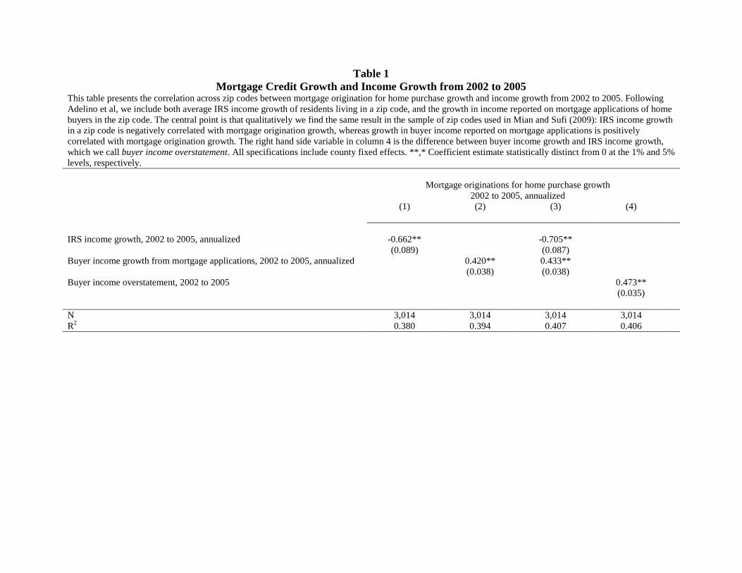
Table 1 Mortgage Credit Growth and Income Growth from 2002 to 2005

This table presents the correlation across zip codes between mortgage origination for home purchase growth and income growth from 2002 to 2005. Following Adelino et al, we include both average IRS income growth of residents living in a zip code, and the growth in income reported on mortgage applications of home buyers in the zip code. The central point is that qualitatively we find the same result in the sample of zip codes used in Mian and Sufi (2009): IRS income growth in a zip code is negatively correlated with mortgage origination growth, whereas growth in buyer income reported on mortgage applications is positively correlated with mortgage origination growth. The right hand side variable in column 4 is the difference between buyer income growth and IRS income growth, which we call buyer income overstatement. All specifications include county fixed effects. **,* Coefficient estimate statistically distinct from 0 at the 1% and 5% levels, respectively. Mortgage originations for home purchase growth

2002 to 2005, annualized

(1) (2) (3) (4) IRS income growth, 2002 to 2005, annualized -0.662** -0.705** (0.089) (0.087) Buyer income growth from mortgage applications, 2002 to 2005, annualized 0.420** 0.433** (0.038) (0.038) Buyer income overstatement, 2002 to 2005 0.473** (0.035) N 3,014 3,014 3,014 3,014 R2 0.380 0.394 0.407 0.406

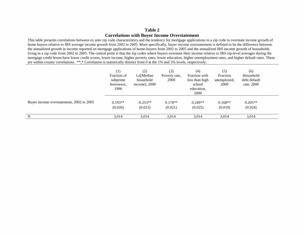
Table 2 Correlations with Buyer Income Overstatement

This table presents correlations between ex ante zip code characteristics and the tendency for mortgage applications in a zip code to overstate income growth of home buyers relative to IRS average income growth from 2002 to 2005. More specifically, buyer income overstatement is defined to be the difference between the annualized growth in income reported on mortgage applications of home-buyers from 2002 to 2005 and the annualized IRS income growth of households living in a zip code from 2002 to 2005. The central point is that the zip codes where buyers overstate their income relative to IRS zip-level averages during the mortgage credit boom have lower credit scores, lower income, higher poverty rates, lower education, higher unemployment rates, and higher default rates. These are within-county correlations. **,* Correlation is statistically distinct from 0 at the 1% and 5% levels, respectively. (1) (2) (3) (4) (5) (6) Fraction of

subprime borrowers,

1996

Ln[Median household

income], 2000

Poverty rate, 2000

Fraction with less than high

school education,

2000

Fraction unemployed,

2000

Household debt default rate, 2000

Buyer income overstatement, 2002 to 2005 0.193** -0.253** 0.178** 0.249** 0.168** 0.205** (0.026) (0.023) (0.021) (0.025) (0.019) (0.024) N 3,014 3,014 3,014 3,014 3,014 3,014

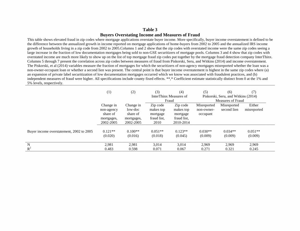
Table 3 Buyers Overstating Income and Measures of Fraud

This table shows elevated fraud in zip codes where mortgage applications overstate buyer income. More specifically, buyer income overstatement is defined to be the difference between the annualized growth in income reported on mortgage applications of home-buyers from 2002 to 2005 and the annualized IRS income growth of households living in a zip code from 2002 to 2005.Columns 1 and 2 show that the zip codes with overstated income were the same zip codes seeing a large increase in the fraction of low documentation mortgages being sold to non-GSE securitizers of mortgage pools. Columns 3 and 4 show that zip codes with overstated income are much more likely to show up on the list of top mortgage fraud zip codes put together by the mortgage fraud detection company InterThinx. Columns 5 through 7 present the correlation across zip codes between measures of fraud from Piskorski, Seru, and Witkins (2014) and income overstatement. The Piskorski, et al (2014) variables measure the fraction of mortgages for which the securitizers of non-agency mortgages misreported whether the loan was a non-owner-occupant loan or whether a second lien was present. The central point is that buyer income overstatement is highest in the same zip codes where (a) an expansion of private label securitization of low documentation mortgages occurred which we know was associated with fraudulent practices, and (b) independent measures of fraud were higher. All specifications include county fixed effects. **,* Coefficient estimate statistically distinct from 0 at the 1% and 5% levels, respectively. (1) (2) (3) (4) (5) (6) (7) InterThinx Measures of

Fraud Piskorski, Seru, and Witkins (2014)

Measures of Fraud

Change in non-agency

share of mortgages, 2002-2005

Change in low-doc share of

mortgages, 2002-2005

Zip code makes top mortgage fraud list,

2010

Zip code makes top mortgage fraud list,

2010-2014

Misreported non-owner-

occupant

Misreported second lien

Either misreported

Buyer income overstatement, 2002 to 2005 0.121** 0.100** 0.051** 0.123** 0.030** 0.034** 0.051** (0.020) (0.016) (0.018) (0.045) (0.009) (0.009) (0.009) N 2,981 2,981 3,014 3,014 2,969 2,969 2,969 R2 0.483 0.598 0.071 0.067 0.271 0.321 0.245

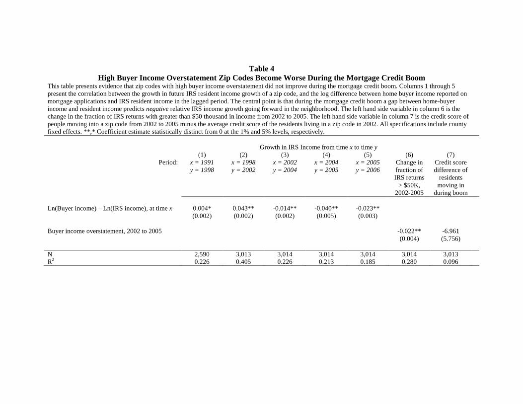
Table 4 High Buyer Income Overstatement Zip Codes Become Worse During the Mortgage Credit Boom

This table presents evidence that zip codes with high buyer income overstatement did not improve during the mortgage credit boom. Columns 1 through 5 present the correlation between the growth in future IRS resident income growth of a zip code, and the log difference between home buyer income reported on mortgage applications and IRS resident income in the lagged period. The central point is that during the mortgage credit boom a gap between home-buyer income and resident income predicts negative relative IRS income growth going forward in the neighborhood. The left hand side variable in column 6 is the change in the fraction of IRS returns with greater than $50 thousand in income from 2002 to 2005. The left hand side variable in column 7 is the credit score of people moving into a zip code from 2002 to 2005 minus the average credit score of the residents living in a zip code in 2002. All specifications include county fixed effects. **,* Coefficient estimate statistically distinct from 0 at the 1% and 5% levels, respectively. Growth in IRS Income from time x to time y (1) (2) (3) (4) (5) (6) (7)

Period: x = 1991 y = 1998

x = 1998 y = 2002

x = 2002 y = 2004

x = 2004 y = 2005

x = 2005 y = 2006

Change in fraction of IRS returns

> $50K, 2002-2005

Credit score difference of

residents moving in

during boom

Ln(Buyer income) – Ln(IRS income), at time x 0.004* 0.043** -0.014** -0.040** -0.023** (0.002) (0.002) (0.002) (0.005) (0.003) Buyer income overstatement, 2002 to 2005 -0.022** -6.961 (0.004) (5.756) N 2,590 3,013 3,014 3,014 3,014 3,014 3,013 R2 0.226 0.405 0.226 0.213 0.185 0.280 0.096

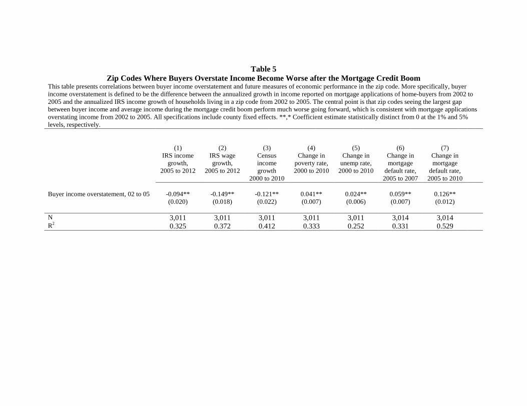
Table 5 Zip Codes Where Buyers Overstate Income Become Worse after the Mortgage Credit Boom

This table presents correlations between buyer income overstatement and future measures of economic performance in the zip code. More specifically, buyer income overstatement is defined to be the difference between the annualized growth in income reported on mortgage applications of home-buyers from 2002 to 2005 and the annualized IRS income growth of households living in a zip code from 2002 to 2005. The central point is that zip codes seeing the largest gap between buyer income and average income during the mortgage credit boom perform much worse going forward, which is consistent with mortgage applications overstating income from 2002 to 2005. All specifications include county fixed effects. **,* Coefficient estimate statistically distinct from 0 at the 1% and 5% levels, respectively. (1) (2) (3) (4) (5) (6) (7) IRS income

growth, 2005 to 2012

IRS wage growth,

2005 to 2012

Census income growth

2000 to 2010

Change in poverty rate, 2000 to 2010

Change in unemp rate,

2000 to 2010

Change in mortgage

default rate, 2005 to 2007

Change in mortgage

default rate, 2005 to 2010

Buyer income overstatement, 02 to 05 -0.094** -0.149** -0.121** 0.041** 0.024** 0.059** 0.126** (0.020) (0.018) (0.022) (0.007) (0.006) (0.007) (0.012) N 3,011 3,011 3,011 3,011 3,011 3,014 3,014 R2 0.325 0.372 0.412 0.333 0.252 0.331 0.529

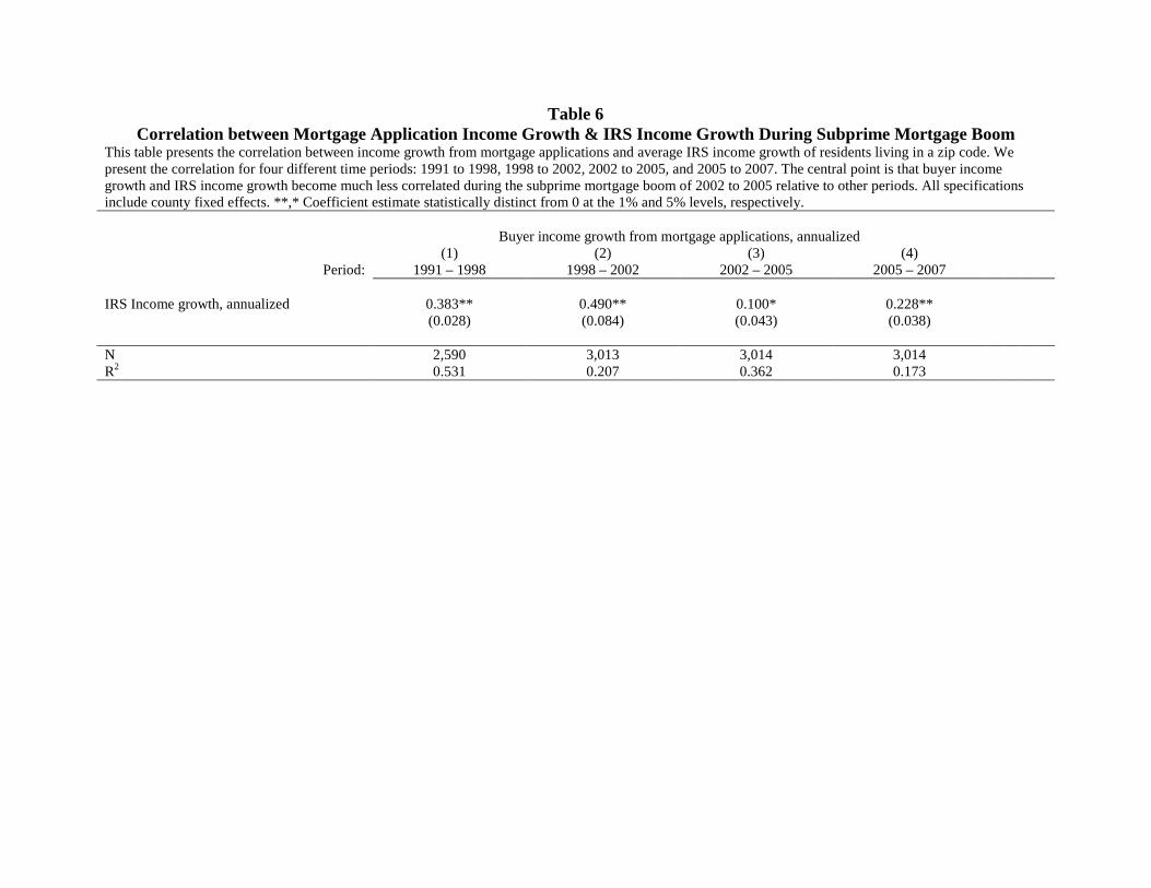
Table 6 Correlation between Mortgage Application Income Growth & IRS Income Growth During Subprime Mortgage Boom

This table presents the correlation between income growth from mortgage applications and average IRS income growth of residents living in a zip code. We present the correlation for four different time periods: 1991 to 1998, 1998 to 2002, 2002 to 2005, and 2005 to 2007. The central point is that buyer income growth and IRS income growth become much less correlated during the subprime mortgage boom of 2002 to 2005 relative to other periods. All specifications include county fixed effects. **,* Coefficient estimate statistically distinct from 0 at the 1% and 5% levels, respectively. Buyer income growth from mortgage applications, annualized (1) (2) (3) (4)

Period: 1991 – 1998 1998 – 2002 2002 – 2005 2005 – 2007 IRS Income growth, annualized 0.383** 0.490** 0.100* 0.228** (0.028) (0.084) (0.043) (0.038) N 2,590 3,013 3,014 3,014 R2 0.531 0.207 0.362 0.173

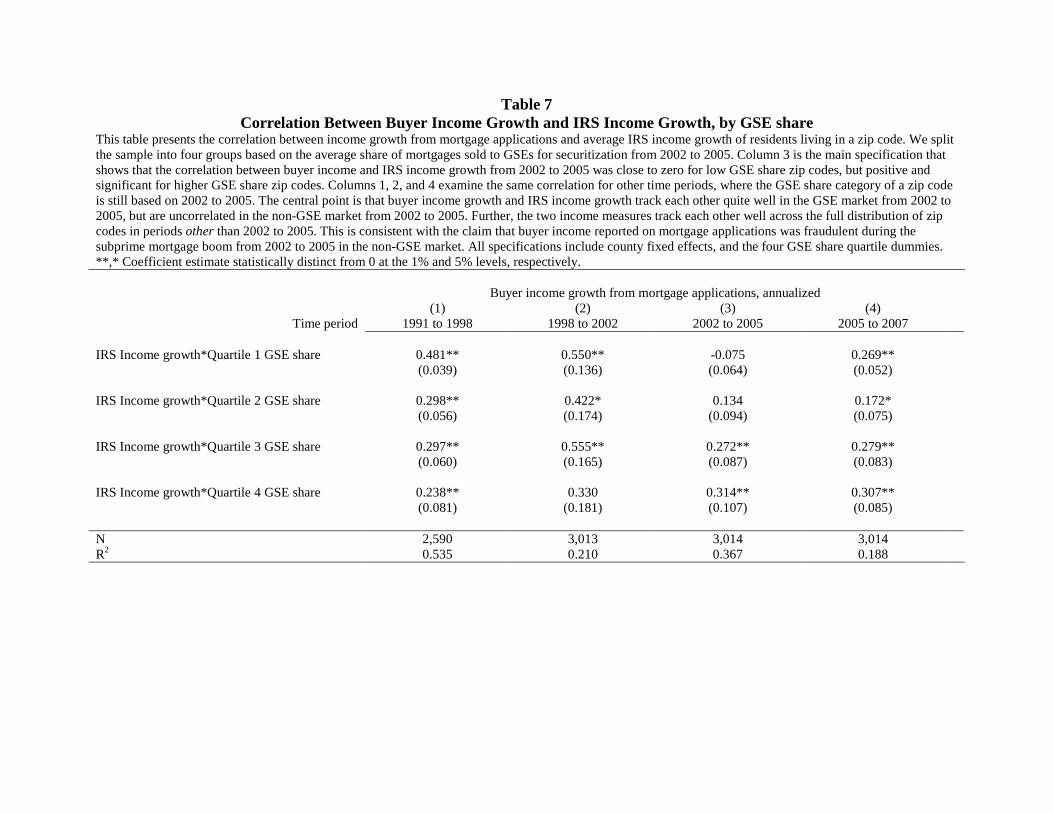
Table 7 Correlation Between Buyer Income Growth and IRS Income Growth, by GSE share

This table presents the correlation between income growth from mortgage applications and average IRS income growth of residents living in a zip code. We split the sample into four groups based on the average share of mortgages sold to GSEs for securitization from 2002 to 2005. Column 3 is the main specification that shows that the correlation between buyer income and IRS income growth from 2002 to 2005 was close to zero for low GSE share zip codes, but positive and significant for higher GSE share zip codes. Columns 1, 2, and 4 examine the same correlation for other time periods, where the GSE share category of a zip code is still based on 2002 to 2005. The central point is that buyer income growth and IRS income growth track each other quite well in the GSE market from 2002 to 2005, but are uncorrelated in the non-GSE market from 2002 to 2005. Further, the two income measures track each other well across the full distribution of zip codes in periods other than 2002 to 2005. This is consistent with the claim that buyer income reported on mortgage applications was fraudulent during the subprime mortgage boom from 2002 to 2005 in the non-GSE market. All specifications include county fixed effects, and the four GSE share quartile dummies. **,* Coefficient estimate statistically distinct from 0 at the 1% and 5% levels, respectively. Buyer income growth from mortgage applications, annualized (1) (2) (3) (4)

Time period 1991 to 1998 1998 to 2002 2002 to 2005 2005 to 2007 IRS Income growth*Quartile 1 GSE share 0.481** 0.550** -0.075 0.269** (0.039) (0.136) (0.064) (0.052) IRS Income growth*Quartile 2 GSE share 0.298** 0.422* 0.134 0.172* (0.056) (0.174) (0.094) (0.075) IRS Income growth*Quartile 3 GSE share 0.297** 0.555** 0.272** 0.279** (0.060) (0.165) (0.087) (0.083) IRS Income growth*Quartile 4 GSE share 0.238** 0.330 0.314** 0.307** (0.081) (0.181) (0.107) (0.085) N 2,590 3,013 3,014 3,014 R2 0.535 0.210 0.367 0.188

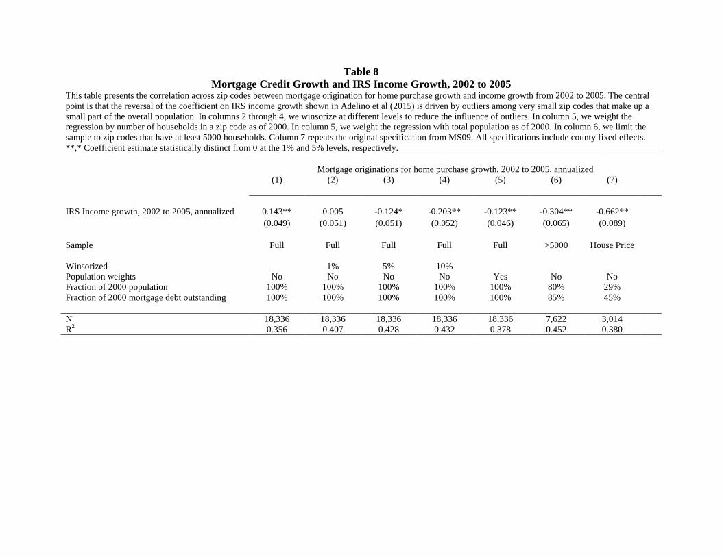
Table 8 Mortgage Credit Growth and IRS Income Growth, 2002 to 2005

This table presents the correlation across zip codes between mortgage origination for home purchase growth and income growth from 2002 to 2005. The central point is that the reversal of the coefficient on IRS income growth shown in Adelino et al (2015) is driven by outliers among very small zip codes that make up a small part of the overall population. In columns 2 through 4, we winsorize at different levels to reduce the influence of outliers. In column 5, we weight the regression by number of households in a zip code as of 2000. In column 5, we weight the regression with total population as of 2000. In column 6, we limit the sample to zip codes that have at least 5000 households. Column 7 repeats the original specification from MS09. All specifications include county fixed effects. **,* Coefficient estimate statistically distinct from 0 at the 1% and 5% levels, respectively. Mortgage originations for home purchase growth, 2002 to 2005, annualized (1) (2) (3) (4) (5) (6) (7) IRS Income growth, 2002 to 2005, annualized 0.143** 0.005 -0.124* -0.203** -0.123** -0.304** -0.662** (0.049) (0.051) (0.051) (0.052) (0.046) (0.065) (0.089) Sample Full Full Full Full Full >5000 House Price Winsorized 1% 5% 10% Population weights No No No No Yes No No Fraction of 2000 population 100% 100% 100% 100% 100% 80% 29% Fraction of 2000 mortgage debt outstanding 100% 100% 100% 100% 100% 85% 45% N 18,336 18,336 18,336 18,336 18,336 7,622 3,014 R2 0.356 0.407 0.428 0.432 0.378 0.452 0.380

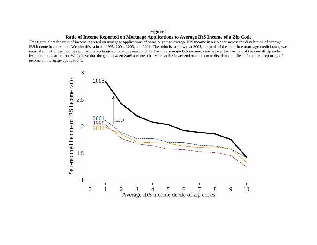
Figure I Ratio of Income Reported on Mortgage Applications to Average IRS Income of a Zip Code

This figure plots the ratio of income reported on mortgage applications of home buyers to average IRS income in a zip code across the distribution of average IRS income in a zip code. We plot this ratio for 1998, 2001, 2005, and 2011. The point is to show that 2005, the peak of the subprime mortgage credit boom, was unusual in that buyer income reported on mortgage applications was much higher than average IRS income, especially at the low part of the overall zip code level income distribution. We believe that the gap between 2005 and the other years at the lower end of the income distribution reflects fraudulent reporting of income on mortgage applications.

fraud?19982001

2011

2005

1

1.5

2

2.5

3Se

lf-re

porte

d in

com

e to

IRS

inco

me

ratio

0 1 2 3 4 5 6 7 8 9 10Average IRS income decile of zip codes

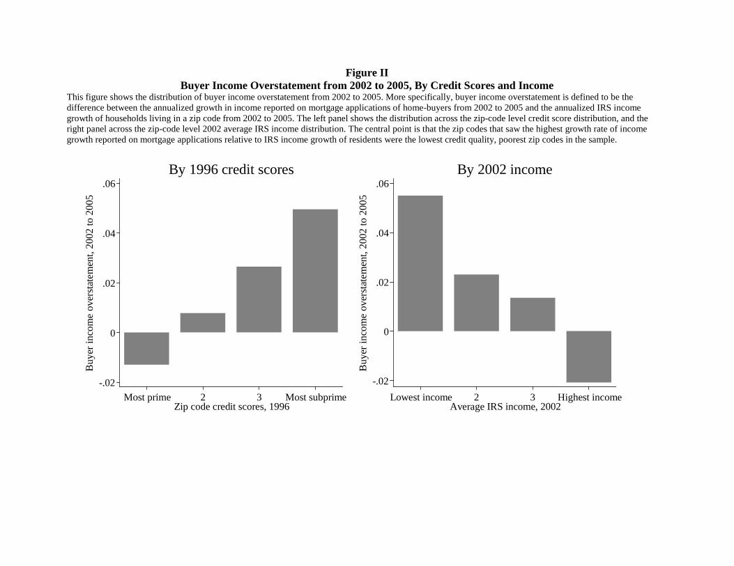
Figure II Buyer Income Overstatement from 2002 to 2005, By Credit Scores and Income

This figure shows the distribution of buyer income overstatement from 2002 to 2005. More specifically, buyer income overstatement is defined to be the difference between the annualized growth in income reported on mortgage applications of home-buyers from 2002 to 2005 and the annualized IRS income growth of households living in a zip code from 2002 to 2005. The left panel shows the distribution across the zip-code level credit score distribution, and the right panel across the zip-code level 2002 average IRS income distribution. The central point is that the zip codes that saw the highest growth rate of income growth reported on mortgage applications relative to IRS income growth of residents were the lowest credit quality, poorest zip codes in the sample.

-.02

0

.02

.04

.06

Buy

er in

com

e ov

erst

atem

ent,

2002

to 2

005

Most prime 2 3 Most subprimeZip code credit scores, 1996

By 1996 credit scores

-.02

0

.02

.04

.06

Buy

er in

com

e ov

erst

atem

ent,

2002

to 2

005

Lowest income 2 3 Highest incomeAverage IRS income, 2002

By 2002 income

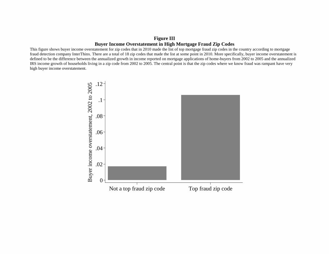
Figure III

Buyer Income Overstatement in High Mortgage Fraud Zip Codes This figure shows buyer income overstatement for zip codes that in 2010 made the list of top mortgage fraud zip codes in the country according to mortgage fraud detection company InterThinx. There are a total of 18 zip codes that made the list at some point in 2010. More specifically, buyer income overstatement is defined to be the difference between the annualized growth in income reported on mortgage applications of home-buyers from 2002 to 2005 and the annualized IRS income growth of households living in a zip code from 2002 to 2005. The central point is that the zip codes where we know fraud was rampant have very high buyer income overstatement.

0

.02

.04

.06

.08

.1

.12B

uyer

inco

me

over

state

men

t, 20

02 to

200

5

Not a top fraud zip code Top fraud zip code

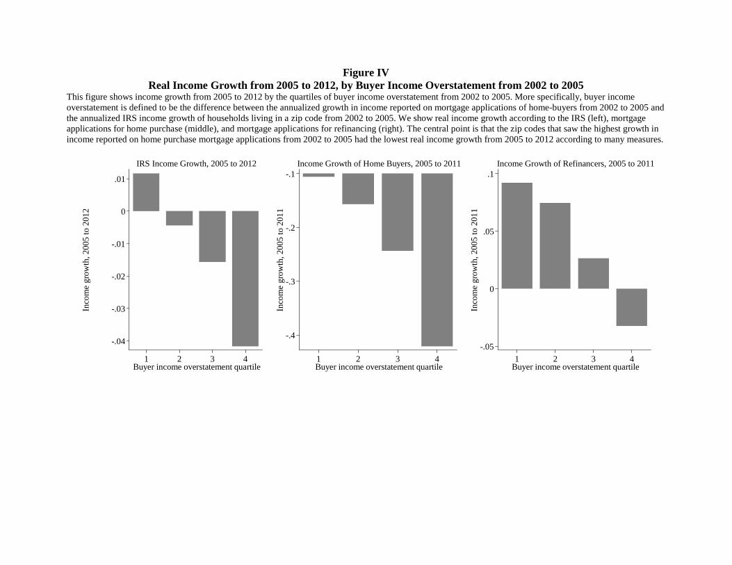
Figure IV Real Income Growth from 2005 to 2012, by Buyer Income Overstatement from 2002 to 2005

This figure shows income growth from 2005 to 2012 by the quartiles of buyer income overstatement from 2002 to 2005. More specifically, buyer income overstatement is defined to be the difference between the annualized growth in income reported on mortgage applications of home-buyers from 2002 to 2005 and the annualized IRS income growth of households living in a zip code from 2002 to 2005. We show real income growth according to the IRS (left), mortgage applications for home purchase (middle), and mortgage applications for refinancing (right). The central point is that the zip codes that saw the highest growth in income reported on home purchase mortgage applications from 2002 to 2005 had the lowest real income growth from 2005 to 2012 according to many measures.

-.04

-.03

-.02

-.01

0

.01

Inco

me

grow

th, 2

005

to 2

012

1 2 3 4Buyer income overstatement quartile

IRS Income Growth, 2005 to 2012

-.4

-.3

-.2

-.1

Inco

me

grow

th, 2

005

to 2

011

1 2 3 4Buyer income overstatement quartile

Income Growth of Home Buyers, 2005 to 2011

-.05

0

.05

.1

Inco

me

grow

th, 2

005

to 2

011

1 2 3 4Buyer income overstatement quartile

Income Growth of Refinancers, 2005 to 2011

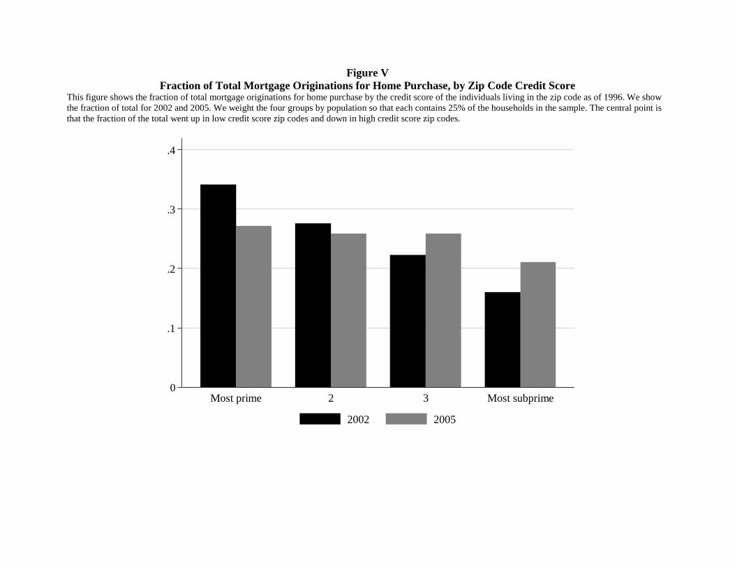
Figure V Fraction of Total Mortgage Originations for Home Purchase, by Zip Code Credit Score

This figure shows the fraction of total mortgage originations for home purchase by the credit score of the individuals living in the zip code as of 1996. We show the fraction of total for 2002 and 2005. We weight the four groups by population so that each contains 25% of the households in the sample. The central point is that the fraction of the total went up in low credit score zip codes and down in high credit score zip codes.

0

.1

.2

.3

.4

Most prime 2 3 Most subprime

2002 2005