four lectures on probabilistic methods for data...

IAS/Park City Mathematics SeriesVolume 00, Pages 000–000S 1079-5634(XX)0000-0

Four lectures on probabilistic methods for data science

Roman Vershynin

Abstract. Methods of high-dimensional probability play a central role in ap-plications for statistics, signal processing, theoretical computer science and re-lated fields. These lectures present a sample of particularly useful tools of high-dimensional probability, focusing on the classical and matrix Bernstein’s inequal-ity and the uniform matrix deviation inequality. We illustrate these tools withapplications for dimension reduction, network analysis, covariance estimation,matrix completion and sparse signal recovery. The lectures are geared towardsbeginning graduate students who have taken a rigorous course in probability butmay not have any experience in data science applications.

Contents

1 Lecture 1: Concentration of sums of independent random variables 11.1 Sub-gaussian distributions 21.2 Hoeffding’s inequality 31.3 Sub-exponential distributions 41.4 Bernstein’s inequality 41.5 Sub-gaussian random vectors 61.6 Johnson-Lindenstrauss Lemma 61.7 Notes 8

2 Lecture 2: Concentration of sums of independent random matrices 92.1 Matrix calculus 92.2 Matrix Bernstein’s inequality 102.3 Community recovery in networks 142.4 Notes 17

3 Lecture 3: Covariance estimation and matrix completion 183.1 Covariance estimation 193.2 Norms of random matrices 223.3 Matrix completion 243.4 Notes 27

4 Lecture 4: Matrix deviation inequality 284.1 Gaussian width 29

Received by the editors December 21, 2016.Partially supported by NSF Grant DMS 1265782 and U.S. Air Force Grant FA9550-14-1-0009.

©0000 (copyright holder)

1

2 Four lectures on probabilistic methods for data science

4.2 Matrix deviation inequality 304.3 Deriving Johnson-Lindenstrauss Lemma 314.4 Covariance estimation 324.5 Underdetermined linear equations 344.6 Sparse recovery 364.7 Notes 37

1. Lecture 1: Concentration of sums of independent random variables

These lectures present a sample of modern methods of high dimensional prob-ability and illustrate these methods with applications in data science. This sampleis not comprehensive by any means, but it could serve as a point of entry intoa branch of modern probability that is motivated by a variety of data-relatedproblems.

To get most out of these lectures, you should have taken a graduate coursein probability, have a good command of linear algebra (including singular valuedecomposition) and be familiar with basic concepts in normed spaces (includingLp spaces).

All of the material of these lectures is covered more systematically, at a slowerpace, and with a wider range of applications, in my forthcoming textbook [53].You may also be interested in two similar tutorials: [51] is focused on randommatrices, and a more advanced text [52] discusses high-dimensional inferenceproblems.

It should be possible to use these lectures for a self-study or group study. Youwill find here many places where you are invited to do some work (marked inthe text e.g. by “check this!”), and you are encouraged to do it to get a bettergrasp of the material. Each lecture ends with a section called “Notes” where youwill find references of the results just discussed, as well as some improvementsand extensions.

We are now ready to start.

Probabilistic reasoning has a major impact on modern data science. There areroughly two ways in which this happens.

• Radnomized algorithms, which perform some operations at random, havelong been developed in computer science and remain very popular. Ran-domized algorithms are among the most effective methods – and some-times the only known ones – for many data problems.

• Random models of data form the usual premise of statistical analysis. Evenwhen the data at hand is deterministic, it is often helpful to think of it as arandom sample drawn from some unknown distribution (“population”).

In this lectures, we will encounter both randomized algorithms and randommodels of data.

Roman Vershynin 3

1.1. Sub-gaussian distributions Before we start discussing probabilistic meth-ods, we will introduce an important class of probability distributions that forms anatural “habitat” for random variables in many theoretical and applied problems.These are sub-gaussian distributions. As the name suggests, we will be lookingat an extension of the most fundamental distribution in probability theory – thegaussian, or normal, distribution N(µ,σ).

It is a good exercise to check that the standard normal random variable X ∼

N(0, 1) satisfies the following basic properties:

Tails: P{|X| > t

}6 2 exp(−t2/2) for all t > 0.

Moments: ‖X‖p := (E |X|p)1/p = O(√p) as p→∞.

MGF of square: 1 E exp(cX2) 6 2 for some c > 0.MGF: E exp(λX) = exp(λ2) for all λ ∈ R.

All these properties tell the same story from four different perspectives. It isnot very difficult to show (although we will not do it here) that for any randomvariable X, not necessarily Gaussian, these four properties are essentially equiva-lent.

Proposition 1.1.1 (Sub-gaussian properties). For a random variable X, the followingproperties are equivalent.2

Tails: P{|X| > t

}6 2 exp(−t2/K2

1) for all t > 0.Moments: ‖X‖p 6 K2

√p for all p > 1.

MGF of square: E exp(X2/K23) 6 2.

Moreover, if EX = 0 then these properties are also equivalent to the following one:

MGF: E exp(λX) 6 exp(λ2K24) for all λ ∈ R.

Random variables that satisfy one of the first three properties (and thus all ofthem) are called sub-gaussian. The best K3 is called the sub-gaussian norm of X, andis usually denoted ‖X‖ψ2 , that is

‖X‖ψ2 := inf{t > 0 : E exp(X2/t2) 6 2

}.

One can check that ‖ · ‖ψ2 indeed defines a norm; it is an example of the generalconcept of the Orlicz norm. Proposition 1.1.1 states that the numbers Ki in all fourproperties are equivalent to ‖X‖ψ2 up to absolute constant factors.

Example 1.1.2. As we already noted, the standard normal random variable X ∼

N(0, 1) is sub-gaussian. Similarly, arbitrary normal random variables X ∼ N(µ,σ)are sub-gaussian. Another example is a Bernoulli random variable X that takesvalues 0 and 1 with probabilities 1/2 each. More generally, any bounded randomvariable X is sub-gaussian. On the contrary, Poisson, exponential, Pareto and

1MGF stands for moment generation function.2The parameters Ki > 0 appearing in these properties can be different. However, they may differfrom each other by at most an absolute constant factor. This means that there exists an absoluteconstant C such that property implies property j with parameter K2 6 CK1, and similarly for everyother pair or properties.


Cauchy distributions are not sub-gaussian. (Verify all these claims; this is notdifficult.)

1.2. Hoeffding’s inequality You may remember from a basic course in probabil-ity that the normal distribution N(µ,σ) has a remarkable property: the sum ofindependent normal random variables is also normal. Here is a version of thisproperty for sub-gaussian distributions.

Proposition 1.2.1 (Sums of sub-gaussians). Let X1, . . . ,XN be independent, meanzero, sub-gaussian random variables. Then

∑Ni=1 Xi is a sub-gaussian, and∥∥∥ N∑

i=1

Xi

∥∥∥2

ψ26 C

N∑i=1

‖Xi‖2ψ2

where C is an absolute constant.3

Proof. Let us bound the moment generating function of the sum for any λ ∈ R:

E exp(λ

N∑i=1

Xi)=

N∏i=1

E exp(λXi) (using independence)

6N∏i=1

exp(Cλ2‖Xi‖2ψ2

) (by last property in Proposition 1.1.1)

= exp(λ2K2) where K2 := C

N∑i=1

‖Xi‖2ψ2

.

Using again the last property in Proposition 1.1.1, we conclude that the sumS =∑Ni=1 Xi is sub-gaussian, and ‖S‖ψ2 6 C1K where C1 is an absolute constant.

The proof is complete. �

Let us rewrite Proposition 1.2.1 in a form that is often more useful in appli-cations, namely as a concentration inequality. To do this, we simply use the firstproperty in Proposition 1.1.1 for the sum

∑Ni=1 Xi. We immediately get the fol-

lowing.

Theorem 1.2.2 (General Hoeffding’s inequality). Let X1, . . . ,XN be independent,mean zero, sub-gaussian random variables. Then, for every t > 0 we have

P{∣∣∣ N∑i=1

Xi

∣∣∣ > t} 6 2 exp(−

ct2∑Ni=1 ‖Xi‖2

ψ2

).

Hoeffding’s inequality controls how far and with what probability can a sumof independent random variables deviate from its mean, which is zero.

3In the future, we will always denote positive absolute constants by C, c, C1, etc. These numbers donot depend on anything. In most cases, one can get good bounds on these constants from the proof,but the optimal constants for each result are rarely known.

Roman Vershynin 5

1.3. Sub-exponential distributions Sub-gaussian distributions form a sufficientlywide class of distributions. Many results in probability and data science areproved nowadays in the for sub-gaussian random variables. Still, as we noted,there are some natural random variables that are not sub-gaussian. For exam-ple, the square X2 of a normal random variable X ∼ N(0, 1) is not sub-gaussian.(Check!) To cover examples like this, we will introduce a similar but weakernotion of sub-exponential distributions.

Proposition 1.3.1 (Sub-exponential properties). For a random variable X, the follow-ing properties are equivalent, in the same sense as in Proposition 1.1.1.

Tails: P{|X| > t

}6 2 exp(−t/K1) for all t > 0.

Moments: ‖X‖p 6 K2p for all p > 1.MGF of square: E exp(|X|/K3) 6 2.

Moreover, if EX = 0 then these properties imply the following one:

MGF: E exp(λX) 6 exp(λ2K24) for |λ| 6 1/K4.

Just like we did for sub-gaussian distributions, we call the best K3 the sub-exponential norm of X and denote it by ‖X‖ψ2 , that is

‖X‖ψ1 := inf {t > 0 : E exp(|X|/t) 6 2} .

All sub-exponential random variables are squares of sub-gaussian random vari-ables. Indeed, inspecting the definitions you will quickly see that

(1.3.2) ‖X2‖ψ1 = ‖X‖2ψ2

.

(Check!)

1.4. Bernstein’s inequality A version of Hoeffding’s inequality for sub-exponentialrandom variables is called Bernstein’s inequality. You may naturally expect to seea sub-exponential tail bound in this result. So it may come as a surprise thatBernstein’s inequality actually has a mixture of two tails – sub-gaussian and sub-exponential. Let us state and prove the inequality first, and then we will commenton the mixture of the two tails.

Theorem 1.4.1 (Bernstein’s inequality). Let X1, . . . ,XN be independent, mean zero,sub-exponential random variables. Then, for every t > 0 we have

P{∣∣∣ N∑i=1

Xi

∣∣∣ > t} 6 2 exp[− cmin

( t2∑Ni=1 ‖Xi‖2

ψ1

,t

maxi ‖Xi‖ψ1

)].

Proof. For simplicity, we will assume that K = 1 and only prove the one-sidedbound (without absolute value); the general case is not much harder. Our ap-proach will be based on bounding the moment generating function of the sumS :=

∑Ni=1 Xi. To see how MGF can be helpful here, choose λ > 0 and use

Markov’s inequality to get

(1.4.2) P{S > t

}= P{

exp(λS) > exp(λt)}6 e−λtE exp(λS).


Recall that S =∑Ni=1 Xi and use independence to express the right side of (1.4.2)

as

e−λtN∏i=1

E exp(λXi).

(Check!) It remains to bound the MGF of each term Xi, and this is a much simplertask. If we choose λ small enough so that

(1.4.3) 0 < λ 6c

maxi ‖Xi‖ψ1

,

then we can use the last property in Proposition 1.3.1 to get

E exp(λXi) 6 exp(Cλ2‖Xi‖2

ψ1

).

Substitute into (1.4.2) and conclude that

P{S > t} 6 exp(−λt+Cλ2σ2

)where σ2 =

∑Ni=1 ‖Xi‖2

ψ1. The left side does not depend on λ while the right side

does. So we can choose λ that minimizes the right side subject to the constraint(1.4.3). When this is done carefully, we obtain the tail bound stated in Bernstein’sinequality. (Do this!) �

Now, why does Bernstein’s inequality has a mixture of two tails? The sub-exponential tail should of course be there. Indeed, even if the entire sum consistedof a single term Xi, the best bound we could hope for would be of the formexp(−ct/‖Xi‖ψ1). The sub-gaussian term could be explained by the central limittheorem, which states that the sum should becomes approximately normal as thenumber of terms N increases to infinity.

Remark 1.4.4 (Bernstein’s inequality for bounded random variables). Suppose therandom variables Xi are uniformly bounded, which is a stronger assumption thanbeing sub-gaussian. Then there is a useful version of Bernstein’s inequality, whichunlike Theorem 1.4.1 is sensitive to the variances of Xi’s. It states that if K > 0 issuch that |Xi| 6 K almost surely for all i, then, for every t > 0, we have

(1.4.5) P{∣∣∣ N∑i=1

Xi

∣∣∣ > t} 6 2 exp(−

−t2/2σ2 +CKt

).

Here σ2 =∑Ni=1 EX2

i is the variance of the sum. This version of Bernstein’sinequality can be proved in essentially the same way as Theorem 1.4.1. We willnot do it here, but a stronger Theorem 2.2.1, which is valid for matrix-valuedrandom variables Xi, will be proved in Lecture 2.

To compare this with Theorem 1.4.1, note that σ2 +CKt 6 2 max(σ2,CKt). Sowe can state this the probability bound (1.4.5) as

2 exp[− cmin

( t2σ2 ,

t

K

)].

Roman Vershynin 7

Just like before, here we also have a mixture of two tails, sub-gaussian andsub-exponential. The sub-gaussian tail is a bit sharper than in Theorem 1.4.1,since it depends on the variances rather than sub-gaussian norms of Xi. The sub-exponential tail, on the other hand, is weaker, since it depends on the sup-normsrather than the sub-exponential norms of Xi.

1.5. Sub-gaussian random vectors The concept of sub-gaussian distributionscan be extended to higher dimensions. Consider a random vector X taking valuesin Rn. We call X a sub-gaussian random vector if all one-dimensional marginals of X,i.e. the random variables 〈X, x〉 for x ∈ Rn, are sub-gaussian. The sub-gaussiannorm of X is defined as

‖X‖ψ2 := supx∈Sn−1

‖ 〈X, x〉 ‖ψ2

where Sn−1 denotes the unit Euclidean sphere in Rn.

Example 1.5.1. Examples of sub-gaussian random distributions in Rn include thestandard normal distribution N(0, In) (why?), the uniform distribution on thecentered Euclidean sphere of radius

√n, the uniform distribution on the cube

{−1, 1}n, and many others. The last example can be generalized: a random vectorX = (X1, . . . ,Xn) with independent and sub-gaussian coordinates is sub-gaussian,with ‖X‖ψ2 6 Cmaxi ‖Xi‖ψ2 .

1.6. Johnson-Lindenstrauss Lemma Concentration inequalities like Hoeffding’sand Bernstein’s are successfully used in the analysis of algorithms. Let us giveone example for the problem of dimension reduction. Suppose we have some datathat is represented as a set of N points in Rn. (Think, for example, of n geneexpressions of N patients.)

We would like to compress the data by representing it in a lower dimensionalspace Rm instead of Rn withm� n. By how much can we reduce the dimensionwithout loosing the important features of the data?

The basic result in this direction is Johnson-Lindenstrauss Lemma. It statesthat a remarkably simple dimension reduction method works – a random linearmap from Rn to Rm with

m ∼ logN,

see Figure 1.6.3. The logarithmic function grows very slowly, so we can usuallyreduce the dimension dramatically.

What exactly is a random linear map? Several models are possible to use.Here we will model such a map using a Gaussian random matrix – an m × nmatrix A with independent N(0, 1) entries. More generally, we can consider anm × n matrix A whose rows are independent, mean zero, isotropic4 and sub-gaussian random vectors in Rn. For example, the entries of A can be independentRademacher entries – those taking values ±1 with equal probabilities.

4A random vector X ∈ Rn is called isotropic if EXXT = In.


Theorem 1.6.1 (Johnson-Lindenstrauss Lemma). Let X be a set of N points in Rn

and ε ∈ (0, 1). Consider an m× n matrix A whose rows are independent, mean zero,isotropic and sub-gaussian random vectors in Rn. Rescale A by defining the “Gaussianrandom projection”5

P :=1√mG.

Assume thatm > Cε−2 logN,

where C is an appropriately large constant that depends only on the sub-gaussian norms ofthe vectors Xi. Then, with high probability (say, 0.99), the map P preserves the distancesbetween all points in X with error ε, that is

(1.6.2) (1 − ε)‖x− y‖2 6 ‖Px− Py‖2 6 (1 + ε)‖x− y‖2 for all x,y ∈ X.

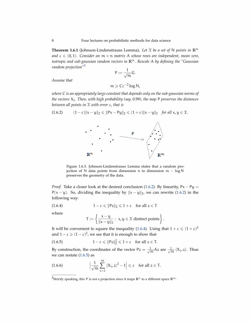
Figure 1.6.3. Johnson-Lindenstrauss Lemma states that a random pro-jection of N data points from dimension n to dimension m ∼ logNpreserves the geometry of the data.

Proof. Take a closer look at the desired conclusion (1.6.2). By linearity, Px− Py =

P(x− y). So, dividing the inequality by ‖x− y‖2, we can rewrite (1.6.2) in thefollowing way:

(1.6.4) 1 − ε 6 ‖Pz‖2 6 1 + ε for all z ∈ T

whereT :=

{x− y

‖x− y‖2: x,y ∈ X distinct points

}.

It will be convenient to square the inequality (1.6.4). Using that 1 + ε 6 (1 + ε)2

and 1 − ε > (1 − ε)2, we see that it is enough to show that

(1.6.5) 1 − ε 6 ‖Pz‖22 6 1 + ε for all z ∈ T .

By construction, the coordinates of the vector Pz = 1√mAz are 1√

m〈Xi, z〉. Thus

we can restate (1.6.5) as

(1.6.6)∣∣∣ 1√m

m∑i=1

〈Xi, z〉2 − 1∣∣∣ 6 ε for all z ∈ T .

5Strictly speaking, this P is not a projection since it maps Rn to a different space Rm.

Roman Vershynin 9

Results like (1.6.6) are often proved by combining concentration and a unionbound. In order to use concentration, we first fix z ∈ T . By assumption, therandom variables 〈Xi, z〉2 − 1 are independent; they have zero mean (use isotropyto check this!), and they are sub-exponential (use (1.3.2) to check this). ThenBernstein’s inequality (Theorem 1.4.1) gives

P

{∣∣∣ 1√m

m∑i=1

〈Xi, z〉2 − 1∣∣∣ > ε} 6 2 exp(−cε2m).

(Check!)Finally, we can unfix z by taking a union bound over all possible z ∈ T :

P

{maxz∈T

∣∣∣ 1√m

m∑i=1

〈Xi, z〉2 − 1∣∣∣ > ε} 6∑

z∈TP

{∣∣∣ 1√m

m∑i=1

〈Xi, z〉2 − 1∣∣∣ > ε}

6 |T | · 2 exp(−cε2m).(1.6.7)

By definition of T , we have |T | 6 N2. So, if we choose m > Cε−2 logN withappropriately large constant C, we can make (1.6.7) bounded by 0.01. The proofis complete. �

1.7. Notes The material presented in Sections 1.1–1.5 is basic and can be founde.g. in [51] and [53] with all the proofs. Bernstein’s and Hoeffding’s inequalitiesthat we covered here are two basic examples of concentration inequalities. Thereare many other useful concentration inequalities for sums of independent randomvariables (e.g. Chernoff’s and Bennett’s) and for more general objects. The text-book [53] is an elementary introduction into concentration; the books [10, 33, 34]offer more comprehensive and more advanced accounts of this area.

The original version of Johnson-Lindenstrauss Lemma was proved in [26]. Theversion we gave here, Theorem 1.6.1, was stated with probability of success 0.99,but an inspection of the proof gives probability 1 − 2 exp(−cε2m) which is muchbetter for large m. A great variety of ramifications and applications of Johnson-Lindenstrauss lemma are known, see e.g. [2, 4, 7, 10, 29, 37].

2. Lecture 2: Concentration of sums of independent random matrices

In the previous lecture we proved Bernstein’s inequality, which quantifies howa sum of independent random variables concentrates about its mean. We willnow study an extension of Bernstein’s inequality to higher dimensions, whichholds for sums of independent random matrices.

2.1. Matrix calculus The key idea of developing a matrix Bernstein’s inequalitywill be to use matrix calculus, which allows us to operate with matrices as withscalars – adding and multiplying them of course, but also comparing matricesand applying functions to matrices. Let us explain this.


We can compare matrices to each other using the notion of being positive semi-definite. Let us focus here on n× n symmetric matrices. If A − B is a positivesemidefinite matrix, which we denote A−B � 0, then we say that A � B (and, ofcourse, B � A). This defines a partial order on the set of n× n symmetric matri-ces. The ream “partial” indicates that, unlike the real numbers, there exist n× nsymmetric matrices A and B that can not be compared. (Give an example whereneither A � B nor B � A!)

Next, let us guess how to measure the magnitude of a matrix A. The magnitudeof a scalar a ∈ R is measured by the absolute value |a|; it is the smallest non-negative number t such that

−t 6 a 6 t.

Extending this reasoning to matrices, we can measure the magnitude of of ann×n symmetric matrix A by the smallest non-negative number t such that6

−tIn � A � tIn.

The smallest t is called the operator norm of A and is denoted ‖A‖. DiagonalizingA, we can see that

(2.1.1) ‖A‖ = max{|λ| : λ is an eigenvalue of A}.

With a little more work (do it!), we can see that ‖A‖ is the norm of A acting as alinear operator on Rn equipped with the Euclidean norm ‖ · ‖2; this is why ‖A‖is called the operator norm. Thus ‖A‖ is the smallest non-negative number Msuch that

‖Ax‖2 6M‖x‖2 for all x ∈ Rn.

Finally, we will need to be able to take functions of matrices. Let f : R → R

be a function and X be an n× n symmetric matrix. We can define f(X) in twoequivalent ways. The spectral theorem allows us to represent X as

X =

n∑i=1

λiuiuTi

where λi are the eigenvalues of X and ui are the corresponding eigenvectors.Then we can simply define

f(X) :=

n∑i=1

f(λi)uiuTi .

Note that f(X) has the same eigenvectors as X, but the eigenvalues change underthe action of f. An equivalent way to define f(X) is using power series. Supposethe function f has a convergent power series expansion about some point x ∈ R,i.e.

f(x) =

∞∑k=1

ak(x− x0)k.

6Here and later, In denotes the n×n identity matrix.

Roman Vershynin 11

Then one can check that the following matrix series converges7 and defines f(X):

f(X) =

∞∑k=1

ak(X−X0)k.

(Check!)

2.2. Matrix Bernstein’s inequality We are now ready to state and prove a re-markable generalization of Bernstein’s inequality for random matrices.

Theorem 2.2.1 (Matrix Bernstein’s inequality). Let X1, . . . ,XN be independent, meanzero, n × n symmetric random matrices, such that ‖Xi‖ 6 K almost surely for all i.Then, for every t > 0 we have

P{∥∥∥ N∑

i=1

Xi

∥∥∥ > t} 6 2n · exp(−

−t2/2σ2 +Kt/3

).

Here σ2 =∥∥∥∑Ni=1 EX2

i

∥∥∥ is the norm of the “matrix variance” of the sum.

The scalar case, where n = 1, is the classical Bernstein’s inequality we statedin (1.4.5). A remarkable feature of matrix Bernstein’s inequality, which makesit especially powerful, is that it does not require any independence of the entries (orthe rows or columns) of Xi; all is needed is that the random matrices Xi beindependent from each other.

We will prove matrix Bernstein’s inequality and give a few applications in thisand next lecture.

Our proof will be based on bounding the moment generating function (MGF)E exp(λS) of the sum S =

∑Ni=1 Xi. Note that to exponentiate the matrix λS in

order to define the matrix MGF, we rely on matrix calculus that we introduced inSection 2.1.

If the terms Xi were scalars, independence would yield the classical fact thatMGF of a product is a product of MGF’s, i.e.

(2.2.2) E exp(λS) = E

N∏i=1

exp(λXi) =N∏i=1

E exp(λXi).

But for matrices, this reasoning breaks down badly, for in general

eX+Y 6= eXeY

even for 2× 2 symmetric matrices X and Y. (Give a counterexample!)Fortunately, there are some trace inequalities that can often serve as proxies

for the missing inequality eX+Y = eXeY . One of such proxies is Golden-Thompsoninequality, which states that

(2.2.3) tr(eX+Y) 6 tr(eXeY)

7The convergence holds in any given metric on the set of matrices, for example in the metric given bythe operator norm. In this series, the terms (X−X0)

k are defined by the usual matrix product.


for any n×n symmetric matrices X and Y. Another result, which we will actuallyuse in the proof of matrix Bernstein’s inequality, is Lieb’s inequality.

Theorem 2.2.4 (Lieb’s inequality). Let H be an n× n symmetric matrix. Then thefunction

f(X) = tr exp(H+ logX)

is concave8 on the space on n×n symmetric matrices.

Note that in the scalar case, where n = 1, the function f in Lieb’s inequality islinear and the result is trivial.

To use Lieb’s inequality in a probabilistic context, we will combine it withthe classical Jensen’s inequality. It states that for any concave function f and arandom matrix X, one has9

(2.2.5) E f(X) 6 f(EX).

Using this for the function f in Lieb’s inequality, we get

E tr exp(H+ logX) 6 tr exp(H+ log EX).

And changing variables to X = eZ, we get the following:

Lemma 2.2.6 (Lieb’s inequality for random matrices). Let H be a fixed n× n sym-metric matrix and Z be an n×n symmetric random matrix. Then

E tr exp(H+Z) 6 tr exp(H+ log E eZ).

Lieb’s inequality is a perfect tool for bounding the MGF of a sum of indepen-dent random variables S =

∑Ni=1 Xi. To do this, let us condition on the random

variables X1, . . . ,XN−1. Apply Lemma 2.2.6 for the fixed matrix H :=∑N−1i=1 λXi

and the random matrix Z := λXi, and afterwards take expectation with respect toX1, . . . ,XN−1. By the law of total expectation, we get

E tr exp(λS) 6 E tr exp[N−1∑i=1

λXi + log E eλXN].

Next, apply Lemma 2.2.6 in a similar manner for H :=∑N−2i=1 λXi + log E eλXN

and Z := λXN−1, and so on. After N times, we obtain:

Lemma 2.2.7 (MGF of a sum of independent random matrices). Let X1, . . . ,XN beindependent n×n symmetric random matrices. Then the sum S =

∑Ni=1 Xi satisfies

E tr exp(λS) 6 tr exp[ N∑i=1

log E eλXi].

8Formally, concavity of f means that f(λX+ (1 − λ)Y) > λf(X) + (1 − λ)f(Y) for all symmetricmatrices X and Y and all λ ∈ [0, 1].9Jensen’s inequality is usually stated for a convex function g and a scalar random variable X, and itreads g(EX) 6 Eg(X). From this, inequality (2.2.5) for concave functions and random matriceseasily follows (Check!).

Roman Vershynin 13

Think of this inequality is a matrix version of the scalar identity (2.2.2). Themain difference is that it bounds the trace of the MGF10 rather the MGF itself.

You may recall from a course in probability theory that the quantity log E eλXi

that appears in this bound is called the cumulant generating function of Xi. Lemma 2.2.7reduces the complexity of our task significantly, for it is much easier to bound thecumulant generating function of each single random variable Xi than to say some-thing about their sum. Here is a simple bound.

Lemma 2.2.8 (Moment generating function). Let X be an n× n symmetric randommatrix. Assume that EX = 0 and ‖X‖ 6 K almost surely. Then, for all 0 < λ < 3/K wehave

E exp(λX) � exp(g(λ)EX2

)where g(λ) =

λ2/21 − λK/3

.

Proof. First, check that the following scalar inequality holds for 0 < λ < 3/K and|x| 6 K:

eλx 6 1 + λx+ g(λ)x2.

Then extend it to matrices using matrix calculus: if 0 < λ < 3/K and ‖X‖ 6 Kthen

eλX � I+ λX+ g(λ)X2.

(Do these two steps carefully!) Finally, take expectation and recall EX = 0 toobtain

E eλX � I+ g(λ)EX2 � exp(g(λ)EX2

).

In the last inequality, we use the matrix version of the scalar inequality 1+ z 6 ez

that holds for all z ∈ R. The lemma is proved. �

Proof of Matrix Bernstein’s inequality. We would like to bound the operator normof the random matrix S =

∑Ni=1 Xi, which, as we know from (2.1.1), is the largest

eigenvalue of S by magnitude. For simplicity of exposition, let us drop the absolutevalue from (2.1.1) and just bound the maximal eigenvalue of S, which we denoteλmax(S). (Once this is done, we can repeat the argument for −S to reinstate theabsolute value. Do this!) So, we are to bound

P{λmax(S) > t

}= P{eλ·λmax(S) > eλt

}(multiply by λ > 0 and exponentiate)

6 e−λt E eλ·λmax(S) (by Markov’s inequality)

= e−λt E λmax(eλS) (check!)

6 e−λt E tr eλS (max of eigenvalues is bounded by the sum)

6 e−λt tr exp[ N∑i=1

log E eλXi]

(use Lemma 2.2.7)

6 tr exp [−λt+ g(λ)Z] (by Lemma 2.2.8)

10Note that the order of expectation and trace can be swapped using linearity.


where

Z :=

N−1∑i=1

EX2i.

It remains to optimize this bound in λ. The minimum is attained for λ =

t/(σ2 +Kt/3). (Check!) Substituting this value for λ, we conclude

P{λmax(S) > t

}6 n · exp

(−

−t2/2σ2 +Kt/3

).

This completes the proof of Theorem 2.2.1. �

Bernstein’s inequality gives a powerful tail bound for ‖∑Ni=1 Xi‖. This easily

implies a useful bound on the expectation:

Corollary 2.2.9 (Expected norm of sum of random matrices). Let X1, . . . ,XN beindependent, mean zero, n× n symmetric random matrices, such that ‖Xi‖ 6 K almostsurely for all i. Then

E

∥∥∥ N∑i=1

Xi

∥∥∥ . σ√logn+K logn

where σ =∥∥∑N

i=1 EX2i

∥∥1/2.

Proof. The link from tail bounds to expectation is provided by the basic identity

(2.2.10) EZ =

∫∞0

P{Z > t

}dt

which is valid for any non-negative random variable Z. (Check it!) Integratingthe tail bound given by matrix Bernstein’s inequality, you will arrive at the expec-tation bound we claimed. (Check!) �

Notice in this corollary a mild, logarithmic, dependence on the ambient di-mension n. As we will see shortly, this can be an important feature in someapplications.

2.3. Community recovery in networks Matrix Bernstein’s inequality has manyapplications. The one we are going to discuss first is for the analysis of net-works. A network can be mathematically represented by graph, a set of n verticeswith edges connecting some of them. For simplicity, we will consider undirectedgraphs where the edges do not have arrows. Real world networks often tend tohave clusters, or communities – subsets of vertices that are connected by unusuallymany edges. (Think, for example, about a friendship network where communi-ties form around some common interests.) An important problem in data scienceis to recover communities from a given network.

We are going to explain one of the simplest methods for community recovery,which is called spectral clustering. But before we introduce it, we will first of allplace a probabilistic model on the networks we consider. In other words, it will beconvenient for us to view networks as random graphs whose edges are formed atrandom. Although not all real-world networks are truly random, this simplistic

Roman Vershynin 15

model can motivate us to develop algorithms that would empirically succeed alsofor real-world networks.

The basic probabilistic model of random graphs is the Erdös-Rényi model.

Definition 2.3.1 (Erdös-Rényi model). Consider a set of n vertices and connect everypair of vertices independently and with fixed probability p. The resulting random graphis said to follow the Erdös-Rényi model G(n,p).

Erdös-Rényi random model is very simple. But is not a good choice if wewant to model a network with communities, for every pair of vertices has thesame chance to be connected. So let us introduce a natural generalization ofErdös-Rényi random model that does allow for community structure:

Definition 2.3.2 (Stochastic block model). Partition a set of n vertices into two subsets(“communities”) with n/2 vertices each, and connect every pair vertices independentlywith probability p if they belong to the same community and q < p if not. The resultingrandom graph is said to follow the stochastic block model G(n,p,q).

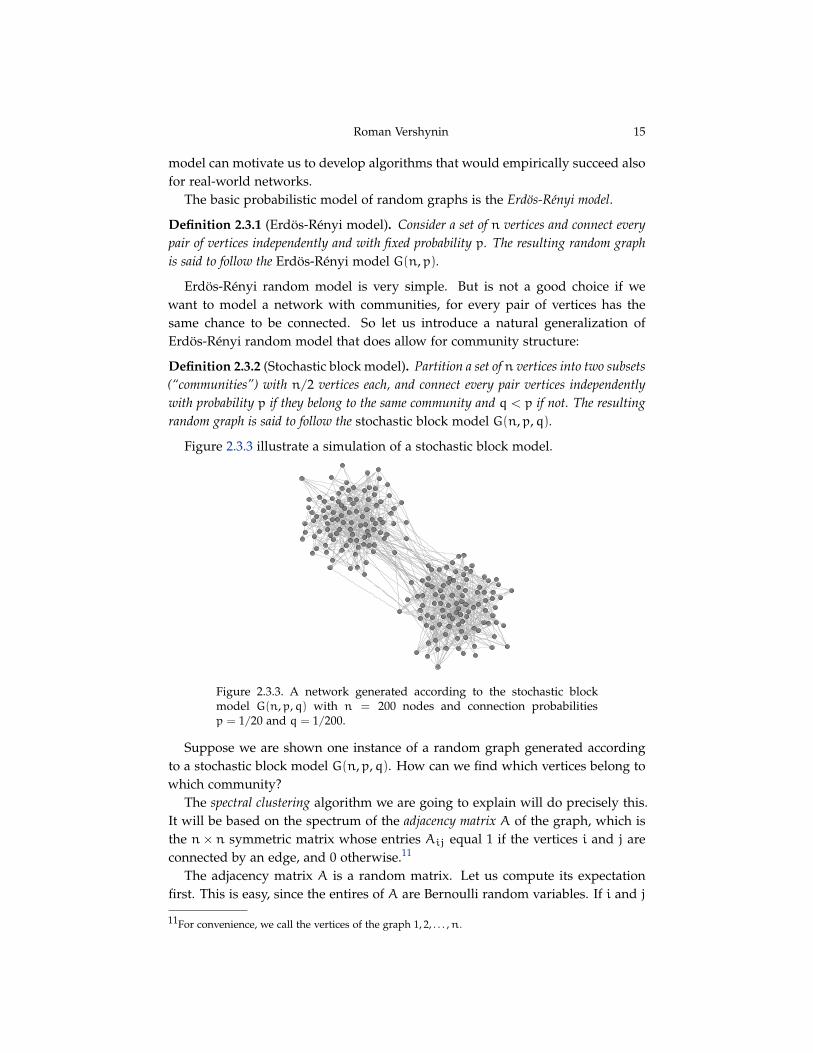
Figure 2.3.3 illustrate a simulation of a stochastic block model.

Figure 2.3.3. A network generated according to the stochastic blockmodel G(n,p,q) with n = 200 nodes and connection probabilitiesp = 1/20 and q = 1/200.

Suppose we are shown one instance of a random graph generated accordingto a stochastic block model G(n,p,q). How can we find which vertices belong towhich community?

The spectral clustering algorithm we are going to explain will do precisely this.It will be based on the spectrum of the adjacency matrix A of the graph, which isthe n× n symmetric matrix whose entries Aij equal 1 if the vertices i and j areconnected by an edge, and 0 otherwise.11

The adjacency matrix A is a random matrix. Let us compute its expectationfirst. This is easy, since the entires of A are Bernoulli random variables. If i and j

11For convenience, we call the vertices of the graph 1, 2, . . . ,n.


belong to the same community then EAij = p and otherwise EAij = q. Thus Ahas block structure: for example, if n = 4 then A looks like this:

EA =

p p q q

p p q q

q q p p

q q p p

(For illustration purposes, we grouped the vertices from each community together.In reality, we do not know in advance how to group them, but we do not needto.)

You will easily check that A has rank 2, and the non-zero eigenvalues and thecorresponding eigenvectors are(2.3.4)

λ1(EA) =(p+ q

2

)n, v1(EA) =

1

1

1

1

; λ2(EA) =(p− q

2

)n, v2(EA) =

1

1

−1

−1

.

(Check!)The eigenvalues and eigenvectors of EA tell us a lot about the community

structure of the underlying graph. Indeed, the first (larger) eigenvalue,

d :=(p+ q

2

)n,

is the expected degree of any vertex of the graph.12 The second eigenvalue tellsus whether there is any community structure at all (which happens when p 6= q

and thus λ2(EA) 6= 0). The first eigenvector v1 is not informative of the structureof the network at all. It is the second eigenvector v2 that tells us exactly how toseparate the vertices into the two communities: the signs of the coefficients of v2

can be used for this purpose.Thus if we know EA, we can recover the community structure of the network

from the signs of the second eigenvector. The problem is that we do not knowEA. Instead, we know the adjacency matrix A. And if, by some chance, A is notfar from EA, we may hope to use the A to approximately recover the communitystructure. So is it true that A ≈ EA? The answer is yes, and we can prove it usingmatrix Bernstein’s inequality.

Theorem 2.3.5 (Concentration of the stochastic block model). LetA be the adjacencymatrix of a G(n,p,q) random graph. Then

E ‖A− EA‖ .√d logn+ logn.

Here d = (p+ q)n/2 is the expected degree.

12The degree of the vertex is the number of edges connected to it.

Roman Vershynin 17

Proof. Let us sketch the argument. To use matrix Bernstein’s inequality, let usbreak A into a sum of independent random matrices

A =∑i,j: i6j

Xij,

where each matrix Xij contains a pair of symmetric entries of A, or one diagonalentry.13 Matrix Bernstein’s inequality obviously applies for the sum

A− EA =∑i6j

(Xij − EXij).

Corollary 2.2.9 gives14

(2.3.6) E ‖A− EA‖ . σ√

logn+K logn

where σ2 =∥∥∑

i6jE(Xij − EXij)2∥∥ and K = maxij ‖Xij − EXij‖. It is a good

exercise to check thatσ2 . d and K 6 2.

(Do it!) Substituting into (2.3.6), we complete the proof. �

How useful is Theorem 2.3.5 for community recovery? Suppose that the net-work is not too sparse, namely

d� logn.

Then‖A− EA‖ .

√d logn while ‖EA‖ = λ1(EA) = d,

which implies that‖A− EA‖ � ‖EA‖.

In other words, A nicely approximates EA: the relative error or approximationis small in the operator norm.

At this point one can classical results from the perturbation theory for matrices,which state that since A and EA are close, their eigenvalues and eigenvectorsmust also be close. The relevant perturbation results are Weyl’s inequality foreigenvalues and Davis-Kahan’s inequality for eigenvectors, which we will not re-produce here. Heuristically, what they give us is

v2(A) ≈ v2(EA) =

1

1

−1

−1

.

13Precisely, if i 6= j, then Xij has all zero entries except the (i, j) and (j, i) entries that equal 1. Ifi = j, the only non-zero entry of Xij is the (i, i).14We will liberally use the notation . to hide constant factors appearing in the inequalities. Thus,a . b means that a 6 Cb for some constant C.


Then we should expect that most of the coefficients of v2(A) be positive on onecommunity and negative on the other. So we can use v2(A) to approximatelyrecover the communities. This method is called spectral clustering:

Spectral Clustering Algorithm. Compute v2(A), the eigenvector corresponding tothe second largest eigenvalue of the adjacency matrix A of the network. Use the signs ofthe coefficients of v2(A) to predict the community membership of the vertices.

We saw that spectral clustering should perform well for stochastic block modelG(n,p,q) if it is not too sparse, namely if the expected degrees satisfy d = (p+

q)n/2� logn.A more careful analysis along these lines, which you should be able to do

yourself with some work, leads to the following more rigorous result.

Theorem 2.3.7 (Guarantees of spectral clustering). Consider a random graph gener-ated according to the stochastic block model G(n,p,q) with p > q, and set a = pn,b = qn. Suppose that

(2.3.8) (a− b)2 � log(n)(a+ b).

Then, with high probability, the spectral clustering algorithm recovers the communitiesup to o(n) misclassified vertices.

2.4. Notes The idea to extend concentration inequalities like Bernstein’s to ma-trices goes back to R. Ahlswede and A. Winter [3]. They used Golden-Thompsoninequality (2.2.3) and proved a slightly weaker form of matrix Bernstein’s inequal-ity than we gave in Section 2.2. R. Oliveira [42, 43] found a way to improvethis argument and gave a result similar to Theorem 2.2.1. The version of matrixBernstein’s inequality we gave here (Theorem 2.2.1) and a proof based on Lieb’sinequality is due to J. Tropp [45].

The survey [46] contains a comprehensive introduction of matrix calculus, aproof of Lieb’s inequality (Theorem 2.2.4), a detailed proof of matrix Bernstein’sinequality (Theorem 2.2.1) and a variety of applications. A proof of Golden-Thompson inequality (2.2.3) can be found in [8, Theorem 9.3.7].

In Section 2.3 we scratched the surface of an interdisciplinary area of net-work analysis. For a systematic introduction into networks, refer to the book[41]. Stochastic block models (Definition 2.3.2) were introduced in [28]. Thecommunity recovery problem in stochastic block models, sometimes also calledcommunity detection problem, has been in the spotlight in the last few years. Avast and still growing body of literature exists on algorithms and theoretical re-sults for community recovery, see the book [41], the survey [21], papers such as[9, 24, 25, 27, 32, 40, 54] and the references therein.

A concentration result similar to Theorem 2.3.5 can be found in [42]; the argu-ment there is also is based on matrix concentration. This theorem is not quite op-timal. For dense networks, where with the expected degree d satisfies d & logn,

Roman Vershynin 19

the concentration inequality in Theorem 2.3.5 can be improved to

(2.4.1) E ‖A− EA‖ .√d.

This improved bound goes back to the original paper [20] which studies the sim-pler Erdös-Rényi model but the results extend to stochastic block models [16]; itcan also be deduced from [6, 27, 32].

If the network is relatively dense, i.e. d & logn, one can improve the guarantee(2.3.8) of spectral clustering in Theorem 2.3.7 to

(a− b)2 � (a+ b).

All one has to do is to use the improved concentration inequality (2.4.1) instead ofTheorem 2.3.5. Furthermore, in this case there exist algorithms that can recoverthe communities exactly, i.e. without any misclassified vertices, and with highprobability, see e.g. [1, 16, 27, 38].

For sparser networks, where d� logn and possibly even d = O(1), relativelylittle algorithms had been known until recently, but now there exist many ap-proaches that provably recover communities in sparse stochastic block models,see e.g. [9, 16, 24, 25, 32, 40, 54].

3. Lecture 3: Covariance estimation and matrix completion

In the last lecture, we proved matrix Bernstein’s inequality and gave an appli-cation for network analysis. We will spend this lecture discussing a couple ofother interesting applications of matrix Bernstein’s inequality. In Section 3.1 wewill work on covariance estimation, a basic problem in high-dimensional statistics.In Section 3.2, we will derive a useful bound on norms random matrices, whichunlike Bernstein’s inequality does not require any boundedness assumptions onthe distribution. We will apply this bound in Section 3.3 for a problem of matrixcompletion, where we are shown a small sample of the entries of a matrix andasked to guess the missing entries.

3.1. Covariance estimation Covariance estimation is a problem of fundamentalimportance in high-dimensional statistics. Suppose we have a sample of datapoints X1, . . . ,XN in Rn. It is often reasonable to assume that these points areindependently sampled from the same probability distribution (or “population”)which is unknown. We would like to learn something useful about this distribu-tion.

Denote by X a random vector that has this (unknown) distribution. The mostbasic parameter of the distribution is the mean EX. One can estimate EX fromthe sample by computing the sample mean 1

N

∑Ni=1 Xi. The law of large numbers

guarantees that the estimate becomes tight as the sample size N grows to infinity,i.e.

1N

N∑i=1

Xi → EX as N→∞.


The next most basic parameter of the distribution is the covariance matrix

Σ := E(X− EX)(X− EX)T.

This is a higher-dimensional version of the usual notion of variance of a randomvariable Z, which is

Var(Z) = E(Z− EZ)2.

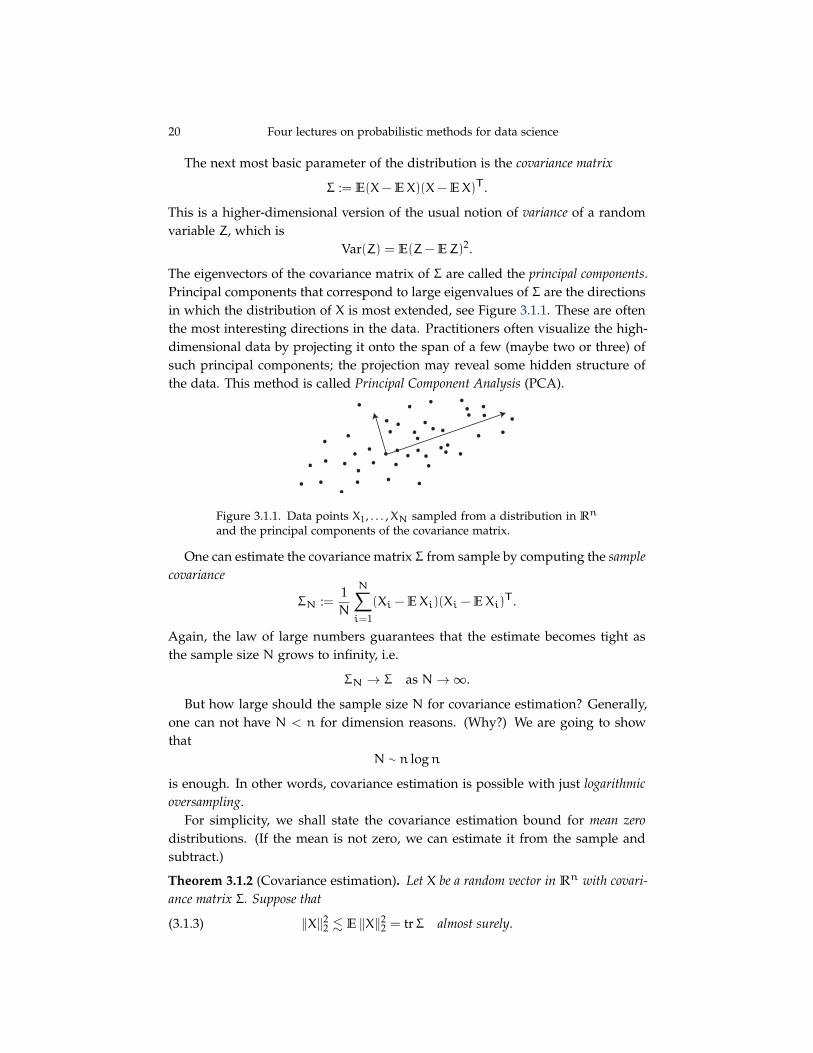
The eigenvectors of the covariance matrix of Σ are called the principal components.Principal components that correspond to large eigenvalues of Σ are the directionsin which the distribution of X is most extended, see Figure 3.1.1. These are oftenthe most interesting directions in the data. Practitioners often visualize the high-dimensional data by projecting it onto the span of a few (maybe two or three) ofsuch principal components; the projection may reveal some hidden structure ofthe data. This method is called Principal Component Analysis (PCA).

Figure 3.1.1. Data points X1, . . . ,XN sampled from a distribution in Rn

and the principal components of the covariance matrix.

One can estimate the covariance matrix Σ from sample by computing the samplecovariance

ΣN :=1N

N∑i=1

(Xi − EXi)(Xi − EXi)T.

Again, the law of large numbers guarantees that the estimate becomes tight asthe sample size N grows to infinity, i.e.

ΣN → Σ as N→∞.

But how large should the sample size N for covariance estimation? Generally,one can not have N < n for dimension reasons. (Why?) We are going to showthat

N ∼ n logn

is enough. In other words, covariance estimation is possible with just logarithmicoversampling.

For simplicity, we shall state the covariance estimation bound for mean zerodistributions. (If the mean is not zero, we can estimate it from the sample andsubtract.)

Theorem 3.1.2 (Covariance estimation). Let X be a random vector in Rn with covari-ance matrix Σ. Suppose that

(3.1.3) ‖X‖22 . E ‖X‖2

2 = trΣ almost surely.

Roman Vershynin 21

Then, for every N > 1, we have

E ‖ΣN − Σ‖ 6 ‖Σ‖(√n logn

N+n lognN

).

Before we pass to the proof, let us note that Theorem 3.1.2 yields the covarianceestimation result we promised. Let ε ∈ (0, 1). If we take a sample of size

N ∼ ε−2n logn,

then we are guaranteed covariance estimation with a good relative error:

E ‖ΣN − Σ‖ 6 ε‖Σ‖.

Proof. Apply matrix Bernstein’s inequality (Corollary 2.2.9) for the sum of inde-pendent random matrices XiXTi − Σ and get

(3.1.4) E ‖ΣN − Σ‖ = 1N

E

∥∥∥ N∑i=1

(XiXTi − Σ)

∥∥∥ . 1N

(σ√

logn+K logn)

where

σ2 =∥∥∥ N∑i=1

E(XiXTi − Σ)2

∥∥∥ = N∥∥E(XXT − Σ)2∥∥

and K is chosen so that

‖XXT − Σ‖ 6 K almost surely.

It remains to bound σ and K. Let us start with σ. We have

E(XXT − Σ)2 = E ‖X‖22XX

T − Σ2 (check by expanding the square)

- tr(Σ) ·EXXT (drop Σ2 and use (3.1.3))

= tr(Σ) · Σ.

Thusσ2 . N tr(Σ)‖Σ‖.

Next, to bound K, we have

‖XXT − Σ‖ 6 ‖X‖22 + ‖Σ‖ (by triangle inequality)

. trΣ+ ‖Σ‖ (using (3.1.3))

6 2 trΣ =: K.

Substitute the bounds on σ and K into (3.1.4) and get

E ‖ΣN − Σ‖ . 1N

(√N tr(Σ)‖Σ‖ logn+ tr(Σ) logn

)To complete the proof, use that trΣ 6 n‖Σ‖ (check this!) and simplify the bound.

�

Remark 3.1.5 (Low-dimensional distributions). Much fewer samples are neededfor covariance estimation for low-dimensional, or approximately low-dimensional,distributions. To measure approximate low-dimensionality we can use the notion


of the stable rank of Σ2. The stable rank of a matrix A is defined as the square ofthe ratio of Frobenius to operator norms:15

r(A) :=‖A‖2

F

‖A‖2 .

The stable rank is always bounded by the usual, linear algebraic rank,

r(A) 6 rank(A),

and it can be much smaller. (Check both claims.)Our proof of Theorem 3.1.2 actually gives

E ‖ΣN − Σ‖ 6 ‖Σ‖(√r logn

N+r lognN

).

wherer = r(Σ1/2) =

trΣ‖Σ‖

.

(Check this!) Therefore, covariance estimation is possible with

N ∼ r logn

samples.

Remark 3.1.6 (The boundedness condition). It is a good exercise to check that ifwe remove the boundedness condition (3.1.3), a nontrivial covariance estimationis impossible in general. (Show this!) But how do we know whether the bound-edness condition holds for data at hand? We may not, but we can enforce thiscondition by truncation. All we have to do is to discard 1% of data points withlargest norms. (Check this accurately, assuming that such truncation does notchange the covariance significantly.)

3.2. Norms of random matrices We have worked a lot with the operator norm ofmatrices, denoted ‖A‖. One may ask if is there a formula that expresses ‖A‖ interms of the entires Aij. Unfortunately, there is no such formula. The operatornorm is a more difficult quantity in this respect than the Frobenius norm, which aswe know can be easily expressed in terms of entries: ‖A‖F = (

∑i,jA

2ij)

1/2.If we can not express of ‖A‖ in terms of the entires, can we at least get a

good estimate? Let us consider n× n symmetric matrices for simplicity. In onedirection, ‖A‖ is always bounded below by the largest Euclidean norm of the rowsAi:

(3.2.1) ‖A‖ > maxi‖Ai‖2 = max

i

(∑j

A2ij

)1/2.

15The Frobenius norm of an n ×m matrix, sometimes also called Hilbert-Schmidt norm, is de-fined as ‖A‖2

F = (∑ni=1∑mj=1A

2ij)

1/2. Equivalently, for an n× n symmetric matrix, ‖A‖2 =

(∑ni=1 λi(A)2)1/2, where λi(A) are the eigenvalues of A. Thus the stable rank of A can be ex-

pressed as r(A) =∑ni=1 λi(A)2/maxi λi(A)2.

Roman Vershynin 23

(Check!) Unfortunately, this bound is sometimes very loose, and the best possibleupper bound is

(3.2.2) ‖A‖ 6√n ·max

i‖Ai‖2.

(Show this bound, and give an example where it is sharp.)Fortunately, for random matrices with independent entries the bound (3.2.2)

can be improved to the point where the upper and lower bounds almost match.

Theorem 3.2.3 (Norms of random matrices without boundedness assumptions).Let A be an n×n symmetric random matrix whose entries on and above the diagonal areindependent, mean zero random variables. Then

E maxi‖Ai‖2 6 E ‖A‖ 6 C logn ·E max

i‖Ai‖2,

where Ai denote the rows of A.

In words, the operator norm of a random matrix is almost determined by thenorm of the rows.

Our proof of this result will be based on matrix Bernstein’s inequality – moreprecisely, Corollary 2.2.9. There is one surprising point. How can we use matrixBernstein’s inequality, which applies only for bounded distributions, to provea result like Theorem 3.2.3 that does not have any boundedness assumptions?We will do this using a trick based on conditioning and symmetrization. Let usintroduce this technique first.

Lemma 3.2.4 (Symmetrization). Let X1, . . . ,XN be independent, mean zero randomvectors in a normed space. Then

12

E

∥∥∥ N∑i=1

εiXi

∥∥∥ 6 E

∥∥∥ N∑i=1

Xi

∥∥∥ 6 2 E

∥∥∥ N∑i=1

εiXi

∥∥∥.

Proof. To prove the upper bound, let (X ′i) be an independent copy of the randomvectors (Xi). Then

E

∥∥∥∑i

Xi

∥∥∥ = E

∥∥∥∑i

Xi − E(∑i

X ′i

)∥∥∥ (since E∑i

X ′i = 0 by assumption)

6 E

∥∥∥∑i

Xi −∑i

X ′i

∥∥∥ (by Jensen’s inequality)

= E

∥∥∥∑i

(Xi −X′i)∥∥∥.

The distribution of the random vectors Yi := Xi−X ′i is symmetric, which meansthat the distributions of Yi and −Y ′i are the same. (Why?) Thus the distributionof the random vectors Yi and εiYi is also the same, for all we do is change thesigns of these vectors at random and independently of the values of the vectors.Summarizing, we can replace Xi −X ′i in the sum above with εi(Xi −X ′i). Thus

E

∥∥∥∑i

Xi

∥∥∥ 6 E

∥∥∥∑i

εi(Xi −X′i)∥∥∥


6 E

∥∥∥∑i

εiXi

∥∥∥+ E

∥∥∥∑i

εiX′i

∥∥∥ (using triangle inequality)

= 2 E

∥∥∥∑i

εiXi

∥∥∥ (the two sums have the same distribution).

This proves the upper bound in the symmetrization inequality. The lower boundcan be proved by a similar argument. (Do this!) �

Proof. We already discussed the lower bound in Theorem 3.2.3. The proof of theupper bound will be based on matrix Bernstein’s inequality.

First, we decompose A in the same way as we did in the proof of Theorem 2.3.5.Thus we represent A as a sum of independent, mean zero, symmetric randommatrices Xij each of which contains a pair of symmetric entries of A (or onediagonal entry):

A =∑i,j: i6j

Zij.

Apply the symmetrization inequality (Lemma 3.2.4) for the random matrices Zijand get

(3.2.5) E ‖A‖ = E

∥∥∥∑i6j

Zij

∥∥∥ 6 2 E

∥∥∥∑i6j

Xij

∥∥∥where we set

Xij := εijZij

and εij are independent Rademacher random variables.Now we condition on A. The random variables Zij become fixed values and all

randomness remains in the Rademacher random variables εij. Note that Xij are(conditionally) bounded almost surely, and this is exactly what we have lacked toapply matrix Bernstein’s inequality. Now we can do it. Corollary 2.2.9 gives16

(3.2.6) Eε

∥∥∥∑i6j

Xij

∥∥∥ . σ√logn+K logn,

where σ2 =∥∥∑

i6jEε X2ij

∥∥ and K = maxi6j ‖Xij‖.A good exercise is to check that

σ . maxi‖Ai‖2 and K . max

i‖Ai‖2.

(Do it!) Substituting into (3.2.6), we get

Eε

∥∥∥∑i6j

Xij

∥∥∥ . logn ·maxi‖Ai‖2.

Finally, we unfix A by taking expectation of both sides of this inequality withrespect to A and using the law of total expectation. The proof is complete. �

16We stick a subscript ε to the expected value to remember that this is a conditional expectation, i.e.we average only with respect to εi.

Roman Vershynin 25

We stated Theorem 3.2.3 for symmetric matrices, but it is simple to extend itto general m×n random matrices A. The bound in this case becomes

(3.2.7) E ‖A‖ 6 C log(m+n) ·(

E maxi‖Ai‖2 + E max

i‖Aj‖2

)where Ai and Aj denote the rows and columns of A. To see this, apply Theo-rem 3.2.3 to the (m+n)× (m+n) symmetric random matrix[

0 A

AT 0

].

(Do this!)

3.3. Matrix completion Consider a fixed, unknown n×n matrix X. Suppose weare shown m randomly chosen entries of X. Can we guess all the missing entries?This important problem is called matrix completion. We will analyze it using thebounds on the norms on random matrices we just obtained.

Obviously, there is no way to guess the missing entries unless we know some-thing extra about the matrix X. So let us assume that X has low rank:

rank(X) =: r� n.

The number of degrees of freedom of an n × n matrix with rank r is O(rn).(Why?) So we may hope that

(3.3.1) m ∼ rn

observed entries of X will be enough to determine X completely. But how?Here we will analyze what is probably the simplest method for matrix com-

pletion. Take the matrix Y that consists of the observed entries of X while allunobserved entries are set to zero. Unlike X, the matrix Y may not have smallrank. Compute the best rank r approximation17 of Y. The result, as we will show,will be a good approximation to X.

But before we show this, let us define sampling of entries more rigorously.Assume each entry of X is shown or hidden independently of others with fixedprobability p. Which entries are shown is decided by independent Bernoullirandom variables

δij ∼ Ber(p) with p :=m

n2

which are often called selectors in this context. The value of p is chosen so thatamong n2 entries of X, the expected number of selected (known) entries is m.Define the n×n matrix Y with entries

Yij := δijXij.

17The best rank r approximation of an n×n matrix A is a matrix B that minimizes the operatornorm ‖A−B‖ or, alternatively, the Frobenius norm ‖A−B‖F (the minimizer turns out to be thesame). One can compute B by truncating the singular value decomposition A =

∑ni=1 siuiv

Ti of

A as follows: B =∑ri=1 siuiv

Ti , where we assume that the singular values si are arranged in the

non-increasing order.


We can assume that we are shown Y, for it is a matrix that contains the observedentries of X while all unobserved entries are replaced with zeros. The followingresult shows how to estimate X based on Y.

Theorem 3.3.2 (Matrix completion). Let X be a best rank r approximation to p−1Y.Then

(3.3.3) E1n‖X−X‖F 6 C log(n)

√rn

m‖X‖∞,

Here ‖X‖∞ = maxi,j |Xij| denotes the maximum magnitude of the entries of X.

Before we prove this result, let us understand what this bound says about thequality of matrix completion. The recovery error is measured in the Frobeniusnorm, and the left side of (3.3.3) is

1n‖X−X‖F =

( 1n2

n∑i,j=1

|Xij −Xij|2)1/2

.

Thus Theorem 3.3.2 controls the average error per entry in the mean-squared sense.To make the error small, let us assume that we have a sample of size

m� rn log2 n,

which is slightly larger than the ideal size we discussed in (3.3.1). This makesC log(n)

√rn/m = o(1) and forces the recovery error to be bounded by o(1)‖X‖∞.

Summarizing, Theorem 3.3.2 says that the expected average error per entry is muchsmaller than the maximal magnitude of the entry of X. This is true for a sample ofalmost optimal size m. The smaller the rank r of the matrix X, the fewer entiresof X we need to see in order to do matrix completion.

Proof of Theorem 3.3.2. Step 1: The error in the operator norm. Let us first boundthe recovery error in the operator norm. Decompose the error into two parts usingtriangle inequality:

‖X−X‖ 6 ‖X− p−1Y‖+ ‖p−1Y −X‖.

Recall that X is a best approximation to p−1Y. Then the first part of the error issmaller than the second part, i.e. ‖X− p−1Y‖ 6 ‖p−1Y −X‖, and we have

(3.3.4) ‖X−X‖ 6 2‖p−1Y −X‖ = 2p‖Y − pX‖.

The entries of the matrix Y − pX,

(Y − pX)ij = (δij − p)Xij,

are independent and mean zero random variables. Thus we can apply the bound(3.2.7) on the norms of random matrices and get

(3.3.5) E ‖Y − pX‖ 6 C logn ·(

E maxi∈[n]

‖(Y − pX)i‖2 + E maxi∈[n]

‖(Y − pX)j‖2).

All that remains is to bound the norms of the rows and columns of Y − pX.This is not difficult if we note that they can be expressed as sums of independent

Roman Vershynin 27

random variables:

‖(Y − pX)i‖22 =

n∑j=1

(δij − p)2X2ij 6

n∑j=1

(δij − p)2 · ‖X‖2∞,

and similarly for columns. Taking expectation and noting that E(δij − p)2 =

Var(δij) = p(1 − p), we get18

(3.3.6) E maxi∈[n]

‖(Y − pX)i‖2 6 (E ‖(Y − pX)i‖22)

1/2 6√pn ‖X‖∞.

This is a good bound, but we need something stronger in (3.3.5). Since the max-imum appears inside the expectation, we need a uniform bound, which will saythat all rows are bounded simultaneously with high probability.

Such uniform bounds are usually proved by applying concentration inequali-ties followed by a union bound. Bernstein’s inequality (1.4.5) yields

P

n∑j=1

(δij − p)2 > tpn

6 exp(−ctpn) for t > 3.

(Check!) This probability can be further bounded by n−ct using the assumptionthat m = pn2 > n logn. A union bound over n rows leads to

P

maxi∈[n]

n∑j=1

(δij − p)2 > tpn

6 n ·n−ct for t > 3.

Integrating this tail, we conclude using (2.2.10) that

E maxi∈[n]

n∑j=1

(δij − p)2 . pn.

(Check!) And this yields the desired bound on the rows,

E maxi∈[n]

‖(Y − pX)i‖2 .√pn,

which is an improvement of (3.3.6) we wanted. We can do similarly for thecolumns. Substituting into (3.3.5), this gives

E ‖Y − pX‖ . log(n)√pn ‖X‖∞.

Then, by (3.3.4), we get

(3.3.7) E ‖X−X‖ . log(n)√n

p‖X‖∞.

Step 2: Passing to Frobenius norm. Now we will need to pass from theoperator to Frobenius norm. This is where we will use for the first (and only)time the rank of X. We know that rank(X) 6 r by assumption and rank(X) 6 rby construction, so rank(X− X) 6 2r. There is a simple relationship between the

18The first bound below that compares the L1 and L2 averages follows from Hölder’s inequality.


operator and Frobenius norms:

‖X−X‖F 6√

2r‖X−X‖.

(Check it!) Take expectation of both sides and use (3.3.7); we get

E ‖X−X‖F 6√

2rE ‖X−X‖ . log(n)√rn

p‖X‖∞.

Dive both sides by n, we can rewrite this bound as

E1n‖X−X‖F . log(n)

√rn

pn2 ‖X‖∞.

But pn2 = m by definition of the sampling probability p. This yields the desiredbound (3.3.3). �

3.4. Notes Theorem 3.1.2 on covariance estimation is a version of [51, Corol-lary 5.52], see also [31]. The logarithmic factor is in general necessary. Thistheorem is a general-purpose result. If one knows some additional structural in-formation about the covariance matrix (such as sparsity), then fewer samples maybe needed, see e.g. [11, 15, 35].

Although the logarithmic factor in Theorem 3.2.3 can not be completely re-moved in general, it can be improved. Our argument actually gives

E ‖A‖ 6 C√

logn ·E maxi‖Ai‖2 +C logn ·E max

ij|Aij|,

Using different methods, one can save an extra√

logn factor and show that

E ‖A‖ 6 CE maxi‖Ai‖2 +C

√logn ·E max

ij|Aij|

(see [6]) andE ‖A‖ 6 C

√logn · log logn ·E max

i‖Ai‖2,

see [48]. (The results in [6, 48] are stated for Gaussian random matrices; the twobounds above can be deduced by using conditioning and symmetrization.) Thesurveys [6, 51] and the textbook [53] present several other useful techniques tobound the operator norm of random matrices.

The matrix completion problem, which we discussed in Section 3.3, has at-tracted a lot of recent attention. E. Candes and B. Recht [13] showed that one canoften achieve exact matrix completion, thus computing the precise values of allmissing values of a matrix, from m ∼ rn log2(n) randomly sampled entries. Forexact matrix completion, one needs an extra incoherence assumption that is notpresent in Theorem 3.3.2. This assumption basically excludes matrices that aresimultaneously sparse and low rank (such as a matrix whose all but one entriesare zero – it would be extremely hard to complete it, since sampling will likelymiss the non-zero entry). Many further results on exact matrix completion areknown, e.g. [14, 17, 23, 49].

Roman Vershynin 29

Theorem 3.3.2 with a simple proof is borrowed from [44]; see also the tutorial[52]. This result only guarantees approximate matrix completion, but it does nothave any incoherence assumptions on the matrix.

4. Lecture 4: Matrix deviation inequality

In this last lecture we will study a new uniform deviation inequality for ran-dom matrices. This result will be a far reaching generalization of Johnson-Linden-strauss Lemma we proved in Lecture 1.

Consider the same setup as in Theorem 1.6.1, where A is an m× n randommatrix whose rows are independent, mean zero, isotropic and sub-gaussian ran-dom vectors in Rn. (If you find it helpful to think in terms of concrete examples,let the entries of A be independent N(0, 1) random variables.) Like in Johnson-Lindenstrauss Lemma, we will be looking at A as a linear transformation fromRn to Rm, and we will be interested in what A does to points in some set in Rn.This time, however, we will allow for infinite sets T ⊂ Rn.

Let us start by analyzing what A does to a single fixed vector x ∈ Rn. We have

E ‖Ax‖22 = E

m∑j=1

⟨Aj, x

⟩2 (where ATj denote the rows of A)

=

m∑j=1

E⟨Aj, x

⟩2 (by linearity)

= m‖x‖22 (using isotropy of Aj).

Further, if we believe that concentration about the mean holds here (and in fact,it does), we should expect that

(4.0.1) ‖Ax‖2 ≈√m ‖x‖2

with high probability.Similarly to Johnson-Lindenstrauss Lemma, our next goal is to make (4.0.1)

hold simultaneously over all vectors x in some fixed set T ⊂ Rn. Precisely, wemay ask – how large is the average uniform deviation:

(4.0.2) E supx∈T

∣∣∣‖Ax‖2 −√m ‖x‖

∣∣∣ ?

This quantity should clearly depend on some notion of the size of T : the largerT , the larger should the uniform deviation be. So, how can we quantify the sizeof T for this problem? In the next section we will do precisely this – introduce aconvenient, geometric measure of the sizes of sets in Rn, which is called Gaussianwidth.

4.1. Gaussian width


Definition 4.1.1. Let T ⊂ Rn be a bounded set, and g be a standard normal randomvector in Rn, i.e. g ∼ N(0, In). Then the quantities

w(T) := E supx∈T〈g, x〉 and γ(T) := E sup

x∈T| 〈g, x〉 |

are called the Gaussian width and of T and the Gaussian complexity of T , respectively.

Gaussian width and Gaussian complexity are closely related. Indeed,19

(4.1.2)w(T) =

12w(T − T) =

12

E supx,y∈T

〈g, x− y〉 = 12

E supx,y∈T

| 〈g, x− y〉 | = 12γ(T − T).

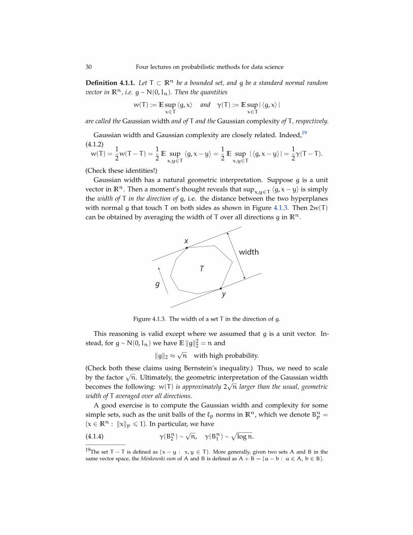
(Check these identities!)Gaussian width has a natural geometric interpretation. Suppose g is a unit

vector in Rn. Then a moment’s thought reveals that supx,y∈T 〈g, x− y〉 is simplythe width of T in the direction of g, i.e. the distance between the two hyperplaneswith normal g that touch T on both sides as shown in Figure 4.1.3. Then 2w(T)can be obtained by averaging the width of T over all directions g in Rn.

x

y

T

width

g

Figure 4.1.3. The width of a set T in the direction of g.

This reasoning is valid except where we assumed that g is a unit vector. In-stead, for g ∼ N(0, In) we have E ‖g‖2

2 = n and

‖g‖2 ≈√n with high probability.

(Check both these claims using Bernstein’s inequality.) Thus, we need to scaleby the factor

√n. Ultimately, the geometric interpretation of the Gaussian width

becomes the following: w(T) is approximately 2√n larger than the usual, geometric

width of T averaged over all directions.A good exercise is to compute the Gaussian width and complexity for some

simple sets, such as the unit balls of the `p norms in Rn, which we denote Bnp =

{x ∈ Rn : ‖x‖p 6 1}. In particular, we have

(4.1.4) γ(Bn2 ) ∼√n, γ(Bn1 ) ∼

√logn.

19The set T − T is defined as {x−y : x,y ∈ T}. More generally, given two sets A and B in thesame vector space, the Minkowski sum of A and B is defined as A+B = {a−b : a ∈A, b ∈ B}.

Roman Vershynin 31

For any finite set T ⊂ Bn2 , we have

(4.1.5) γ(T) .√

log |T |.

The same holds for Gaussian width w(T). (Check these facts!)A look a these examples reveals that the Gaussian width captures some non-

obvious geometric qualities of sets. Of course, the fact that the Gaussian width ofthe unit Euclidean ball Bn2 is or order

√n is not surprising: the usual, geometric

width in all directions is 2 and the Gaussian width is about√n times that. But

it may be surprising that the Gaussian width of the `1 ball Bn1 is much smaller,and so is the width of any finite set T (unless the set has exponentially largecardinality). As we will see later, Gaussian width nicely captures the geometricsize of “the bulk” of a set.

4.2. Matrix deviation inequality Now we are ready to answer the question weasked in the beginning of this lecture: what is the magnitude of the uniform de-viation (4.0.2)? The answer is surprisingly simple: it is bounded by the Gaussiancomplexity of T . The proof is not too simple however, and we will skip it.

Theorem 4.2.1 (Matrix deviation inequality). Let A be an m×n matrix whose rowsAi are independent, isotropic and sub-gaussian random vectors in Rn. Let T ⊂ Rn be afixed bounded set. Then

E supx∈T

∣∣∣‖Ax‖2 −√m‖x‖2

∣∣∣ 6 CK2γ(T)

where K = maxi ‖Ai‖ψ2 is the maximal sub-gaussian norm20 of the rows of A.

Remark 4.2.2 (Tail bound). It is often useful to have results that hold with highprobability rather than in expectation. There exists a high-probability version ofmatrix deviation inequality, and it states the following. Let u > 0. Then the event

(4.2.3) supx∈T

∣∣∣‖Ax‖2 −√m‖x‖2

∣∣∣ 6 CK2 [γ(T) + u · rad(T)]

holds with probability at least 1 − 2 exp(−u2). Here rad(T) is the radius of T ,defined as

rad(T) := supx∈T‖x‖2.

Since rad(T) . γ(T) (check!) we can continue the bound (4.2.3) by

. K2uγ(T)

for all u > 1. This is a weaker but still a useful inequality. For example, we canuse it to bound all higher moments of the deviation:

(4.2.4)(

E supx∈T

∣∣∣‖Ax‖2 −√m‖x‖2

∣∣∣p)1/p6 CpK

2γ(T)

where Cp 6 C√p for p > 1. (Check this using Proposition 1.1.1.)

20A definition of the sub-gaussian norm of a random vector was given in Section 1.5. Foe example, ifA is a Gaussian random matrix with independent N(0, 1) entries, then K is an absolute constant.


Remark 4.2.5 (Deviation of squares). It is sometimes helpful to bound the devia-tion of the square ‖Ax‖2

2 rather than ‖Ax‖2 itself. We can easily deduce the devia-tion of squares by using the identity a2 −b2 = (a−b)2 + 2b(a−b) for a = ‖Ax‖2

and b =√m‖x‖2. Doing this, we conclude that

(4.2.6) E supx∈T

∣∣∣‖Ax‖22 −m‖x‖

22

∣∣∣ 6 CK4γ(T)2 +CK2√m rad(T)γ(T).

(Do this calculation using (4.2.4) for p = 2.) We will use this bound in Section 4.4.

Matrix deviation inequality has many consequences. We will explore some ofthen now.

4.3. Deriving Johnson-Lindenstrauss Lemma We started this lecture by promis-ing a result that is more general than Johnson-Lindenstrauss Lemma. So let usshow how to quickly derive Johnson-Lindenstrauss from the matrix deviationinequality. Theorem 1.6.1 from Theorem 4.2.1.

Assume we are in the situation of Johnson-Lindenstrauss Lemma (Theorem 1.6.1).Given a set X ⊂ R, consider the normalized difference set

T :={ x− y

‖x− y‖2: x,y ∈ X distinct vectors

}.

Then T is a finite subset of the unit sphere of Rn, and thus (4.1.5) gives

γ(T) .√

log |T | 6√

log |X|2 .√

log |X|.

Matrix deviation inequality (Theorem 4.2.1) then yields

supx,y∈X

∣∣∣‖A(x− y)‖2

‖x− y‖2−√m∣∣∣ .√logN 6 ε

√m.

with high probability, say 0.99. (To pass from expectation to high probability, wecan use Markov’s inequality. To get the last bound, we use the assumption on min Johnson-Lindenstrauss Lemma.)

Multiplying both sides by ‖x−y‖2/√m, we can write the last bound as follows.

With probability at least 0.99, we have

(1 − ε)‖x− y‖2 61√m‖Ax−Ay‖2 6 (1 + ε)‖x− y‖2 for all x,y ∈ X.

This is exactly the consequence of Johnson-Lindenstrauss lemma.The argument based on matrix deviation inequality, which we just gave, can

be easily extended for infinite sets. It allows one to state a version of Johnson-Lindenstrauss lemma for general, possibly infinite, sets, which depends on theGaussian complexity of T rather than cardinality. (Try to do this!)

4.4. Covariance estimation In Section 3.1, we introduced the problem of covari-ance estimation, and we showed that

N ∼ n logn

samples are enough to estimate the covariance matrix of a general distributionin Rn. We will now show how to do better if the distribution is sub-gaussian.

Roman Vershynin 33

(Recall Section 1.5 for the definition of sub-gaussian random vectors.) In this case,we can get rid of the logarithmic oversampling and the boundedness condition(3.1.3).

Theorem 4.4.1 (Covariance estimation for sub-gaussian distributions). Let X be arandom vector in Rn with covariance matrix Σ. Suppose X is sub-gaussian, and morespecifically

(4.4.2) ‖ 〈X, x〉 ‖ψ2 . ‖ 〈X, x〉 ‖L2 = ‖Σ1/2x‖2 for any x ∈ Rn.

Then, for every N > 1, we have

E ‖ΣN − Σ‖ . ‖Σ‖(√ n

N+n

N

).

This result implies that if, for ε ∈ (0, 1), we take a sample of size

N ∼ ε−2n,

then we are guaranteed covariance estimation with a good relative error:

E ‖ΣN − Σ‖ 6 ε‖Σ‖.

Proof. Since we are going to use Theorem 4.2.1, we will need to first bring therandom vectors X,X1, . . . ,XN to the isotropic position. This can be done by asuitable linear transformation. You will easily check that there exists an isotropicrandom vector Z such that

X = Σ1/2Z.

(For example, Σ has full rank, set Z := Σ−1/2X. Check the general case.) Similarly,we can find independent and isotropic random vectors Zi such that

Xi = Σ1/2Zi, i = 1, . . . ,N.

The sub-gaussian assumption (4.4.2) then implies that

‖Z‖ψ2 . 1.

(Check!) Then

‖ΣN − Σ‖ = ‖Σ1/2RNΣ1/2‖ where RN :=

1N

N∑i=1

ZiZTi − In.

The operator norm of a symmetric n× n matrix A can be computed by maxi-mizing the quadratic form over the unit sphere: ‖A‖ = maxx∈Sn−1 | 〈Ax, x〉 |. (Tosee this, recall that the operator norm is the biggest eigenvalue of A in magni-tude.) Then

‖ΣN − Σ‖ = maxx∈Sn−1

⟨Σ1/2RNΣ

1/2x, x⟩= maxx∈T〈RNx, x〉

where T is the ellipsoidT := Σ1/2Sn−1.


Recalling the definition of RN, we can rewrite this as

‖ΣN − Σ‖ = maxx∈T

∣∣∣ 1N

N∑i=1

〈Zi, x〉2 − ‖x‖22

∣∣∣ = 1N

maxx∈T

∣∣‖Ax‖22 −N‖x‖

22∣∣.

Now we apply the matrix deviation inequality for squares (4.2.6) and concludethat

‖ΣN − Σ‖ . 1N

(γ(T)2 +

√N rad(T)γ(T)

).

(Do this calculation!) The radius and Gaussian width of the ellipsoid T are easyto compute:

rad(T) = ‖Σ‖1/2 and γ(T) 6 (trΣ)1/2.

Substituting, we get

‖ΣN − Σ‖ . 1N

(trΣ+

√N‖Σ‖ trΣ

).

To complete the proof, use that trΣ 6 n‖Σ‖ (check this!) and simplify the bound.�

Remark 4.4.3 (Low-dimensional distributions). Similarly to Section 3.1, we canshow that much fewer samples are needed for covariance estimation of low-dimensional sub-gaussian distributions. Indeed, the proof of Theorem 4.4.1 ac-tually yields

(4.4.4) E ‖ΣN − Σ‖ 6 ‖Σ‖(√ r

N+r

N

)where

r = r(Σ1/2) =trΣ‖Σ‖

is the stable rank of Σ1/2. This means that covariance estimation for is possiblewith

N ∼ r

samples.

4.5. Underdetermined linear equations We will give one more application ofthe matrix deviation inequality – this time, to the area of high dimensional in-ference. Suppose we need to solve a severely undetermined system of linearequations: say, we have m equations in n � m variables. Let us write it in thematrix form as

y = Ax

where A is a given m× n matrix, y ∈ Rm is a given vector and x ∈ Rn is anunknown vector. We would like to compute x from A and y.

When the linear system is underdetermined, we can not find x with any ac-curacy, unless we know something extra about x. So, let us assume that we dohave some a-priori information. We can describe this situation mathematically byassuming that

x ∈ K

Roman Vershynin 35

where K ⊂ Rn is some known set in Rn that describes anything that we knowabout x a-priori. (Admittedly, we are operating on a high level of generality here.If you need a concrete example, we will consider it in Section 4.6.)

Summarizing, here is the problem we are trying to solve. Determine a solu-tion x = x(A,y,K) to the undetermined linear equation y = Ax as accurately aspossible, assuming that x ∈ K.

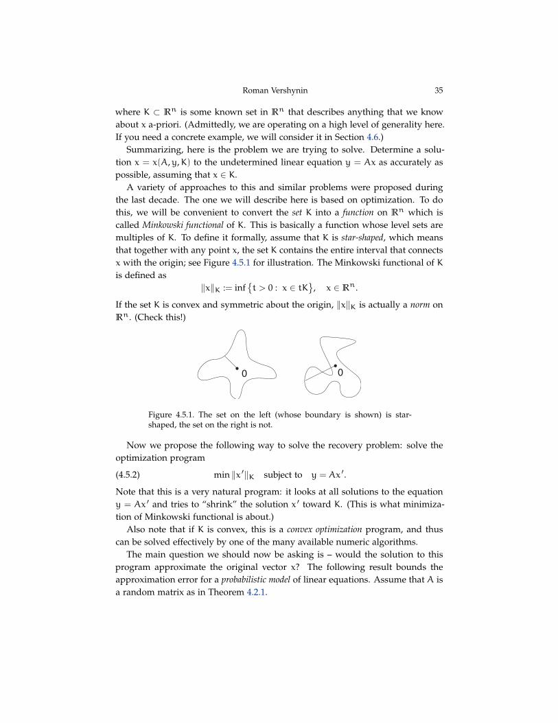
A variety of approaches to this and similar problems were proposed duringthe last decade. The one we will describe here is based on optimization. To dothis, we will be convenient to convert the set K into a function on Rn which iscalled Minkowski functional of K. This is basically a function whose level sets aremultiples of K. To define it formally, assume that K is star-shaped, which meansthat together with any point x, the set K contains the entire interval that connectsx with the origin; see Figure 4.5.1 for illustration. The Minkowski functional of Kis defined as

‖x‖K := inf{t > 0 : x ∈ tK

}, x ∈ Rn.

If the set K is convex and symmetric about the origin, ‖x‖K is actually a norm onRn. (Check this!)

0 0

Figure 4.5.1. The set on the left (whose boundary is shown) is star-shaped, the set on the right is not.

Now we propose the following way to solve the recovery problem: solve theoptimization program

(4.5.2) min ‖x ′‖K subject to y = Ax ′.

Note that this is a very natural program: it looks at all solutions to the equationy = Ax ′ and tries to “shrink” the solution x ′ toward K. (This is what minimiza-tion of Minkowski functional is about.)

Also note that if K is convex, this is a convex optimization program, and thuscan be solved effectively by one of the many available numeric algorithms.

The main question we should now be asking is – would the solution to thisprogram approximate the original vector x? The following result bounds theapproximation error for a probabilistic model of linear equations. Assume that A isa random matrix as in Theorem 4.2.1.


Theorem 4.5.3 (Recovery by optimization). The solution x of the optimization pro-gram (4.5.2) satisfies21

E ‖x− x‖2 .w(K)√m

,

where w(K) is the Gaussian width of K.

Proof. Both the original vector x and the solution x are feasible vectors for theoptimization program (4.5.2). Then

‖x‖K 6 ‖x‖K (since x minimizes the Minkowski functional)

6 1 (since x ∈ K).

Thus both x, x ∈ K.We also know that Ax = Ax = y, which yields

(4.5.4) A(x− x) = 0.

Let us apply matrix deviation inequality (Theorem 4.2.1) for T := K − K. Itgives

E supu,v∈K

∣∣∣‖A(u− v)‖2 −√m ‖u− v‖2

∣∣∣ . γ(K−K) = 2w(K),

where we used (4.1.2) in the last identity. Substitute u = x and v = x here. Wemay do this since, as we noted above, both these vectors belong to K. But thenthe term ‖A(u− v)‖2 will be equal zero by (4.5.4). It disappears from the bound,and we get

E√m ‖x− x‖2 . w(K).

Dividing both sides by√m we complete the proof. �

Theorem 4.5.3 says that a signal x ∈ K can be efficiently recovered from

m ∼ w(K)2

random linear measurements.

4.6. Sparse recovery Let us illustrate Theorem 4.5.3 with an important specificexample of the feasible set K.

Suppose we know that the signal x is sparse, which means that only few coordi-nates of x are nonzero. As before, our task is to recover x from the random linearmeasurements given by the vector

y = Ax,

where A is an m× n random matrix. This is a basic example of sparse recoveryproblems, which are ubiquitous in various disciplines.

The number of nonzero coefficients of a vector x ∈ Rn, or the sparsity of x,is often denoted ‖x‖0. This is similar to the notation for the `p norm ‖x‖p =

21Here and in other similar results, the notation . will hide possible dependence on the sub-gaussiannorms of the rows of A.

Roman Vershynin 37

(∑ni=1 |xi|

p)1/p, and for a reason. You can quickly check that

(4.6.1) ‖x‖0 = limp→0‖x‖p

(Do this!) Keep in mind that neither ‖x‖0 nor ‖x‖p for 0 < p < 1 are actuallynorms on Rn, since they fail triangle inequality. (Give an example.)

Let us go back to the sparse recovery problem. Our first attempt to recover xis to try the following optimization problem:

(4.6.2) min ‖x ′‖0 subject to y = Ax ′.

This is sensible because this program selects the sparsest feasible solution. Onecan show that the program performs well. But there is an implementation caveat:the function f(x) = ‖x‖0 is highly non-convex and even discontinuous. There issimply no known algorithm to solve the optimization problem (4.6.2) efficiently.

To overcome this difficulty, let us turn to the relation (4.6.1) for an inspiration.What if we replace ‖x‖0 in the optimization problem (4.6.2) by ‖x‖p with p > 0?The smallest p for which f(x) = ‖x‖p is a genuine norm (and thus a convexfunction on Rn) is p = 1. So let us try

(4.6.3) min ‖x ′‖1 subject to y = Ax ′.

This is a convexification of the non-convex program (4.6.2), and a variety of nu-meric convex optimization methods are available to solve it efficiently.

We will now show that `1 minimization works nicely for sparse recovery. Asbefore, we assume that A is a random matrix as in Theorem 4.2.1.

Theorem 4.6.4 (Sparse recovery by optimization). Assume that an unknown vectorx ∈ Rn has at most s non-zero coordinates, i.e. ‖x‖0 6 s. The solution x of theoptimization program (4.6.3) satisfies

E ‖x− x‖2 .

√s lognm

‖x‖2.

Proof. Since ‖x‖0 6 s, Cauchy-Schwarz inequality shows that

(4.6.5) ‖x‖1 6√s ‖x‖2.

(Check!) Denote the unit ball of the `1 norm in Rn by Bn1 , i.e. Bn1 := {x ∈ Rn :

‖x‖1 6 1}. Then we can rewrite (4.6.5) as the inclusion

x ∈√s ‖x‖2 ·Bn1 := K.

Apply Theorem 4.5.3 for this set K. We noted the Gaussian width of Bn1 in (4.1.4),so

w(K) =√s ‖x‖2 ·w(Bn1 ) 6

√s ‖x‖2 · γ(Bn1 ) 6

√s ‖x‖2 ·

√logn.

Substitute this is Theorem 4.5.3 and complete the proof. �

Theorem 4.6.4 says that an s-sparse signal x ∈ Rn can be efficiently recoveredfrom

m ∼ s logn

38 References

random linear measurements.

4.7. Notes For a more thorough introduction to Gaussian width and its role inhigh-dimensional estimation, refer to the tutorial [52] and the textbook [53]; seealso [5].

Matrix deviation inequality (Theorem 4.2.1) is borrowed from [36]. In the spe-cial case where A is a Gaussian random matrix, this result follows from the workof G. Schechtman [50]. In the general case of sub-gaussian distributions, ear-lier variants of Theorem 4.2.1 were proved by B. Klartag and S. Mendelson [30],S. Mendelson, A. Pajor and N. Tomczak-Jaegermann [39] and S. Dirksen [19].

Theorem 4.4.1 for covariance estimation can be proved alternatively using moreelementary tools (Bernstein’s inequality and ε-nets), see [51]. However, no knownelementary approach exists for the low-rank covariance estimation discussed inRemark 4.4.3. The bound (4.4.4) was proved by V. Koltchinskii and K. Lounici[31] by a different method.

In Section 4.5, we scratched the surface of a recently developed area of sparsesignal recovery, which is also called compressed sensing. Our presentation thereessentially follows the tutorial [52]. Theorem 4.6.4 can be improved: if we take

m & s log(n/s)

measurements, then with high probability the optimization program (4.6.3) recov-ers the unknown signal x exactly, i.e.

x = x.

First results of this kind were proved by J. Romberg, E. Candes and T. Tao [12]and a great number of further developments followed; refer e.g. to the book [22]and the chapter in [18] for an introduction into this reach area.

References[1] E. Abbe, A. S. Bandeira, G. Hall. Exact recovery in the stochastic block model, IEEE Transactions on

Information Theory 62 (2016), 471–487. 18[2] D. Achlioptas, Database-friendly random projections: Johnson-Lindenstrauss with binary coins, Journal

of Computer and System Sciences, 66 (2003), 671–687. 9[3] R. Ahlswede, A. Winter, Strong converse for identification via quantum channels, IEEE Trans. Inf.

Theory 48 (2002), 569–579. 17[4] N. Ailon, B. Chazelle, Approximate nearest neighbors and the fast Johnson-Lindenstrauss transform,

Proceedings of the 38th Annual ACM Symposium on Theory of Computing. New York: ACMPress, 2006. pp. 557–563. 9

[5] D. Amelunxen, M. Lotz, M. McCoy, J. Tropp, Living on the edge: phase transitions in convex programswith random data, Inf. Inference 3 (2014), 224–294. 37

[6] A. Bandeira, R. van Handel, Sharp nonasymptotic bounds on the norm of random matrices with inde-pendent entries, Ann. Probab. 44 (2016), 2479–2506. 18, 28

[7] R. Baraniuk, M. Davenport, R. DeVore, M. Wakin, A simple proof of the restricted isometry propertyfor random matrices, Constructive Approximation, 28 (2008), 253–263. 9

[8] R. Bhatia, Matrix Analysis. Graduate Texts in Mathematics, vol. 169. Springer, Berlin, 1997. 18[9] C. Bordenave, M. Lelarge, L. Massoulie, |em Non-backtracking spectrum of random graphs:

community detection and non-regular Ramanujan graphs, Annals of Probability, to appear. 18

References 39

[10] S. Boucheron, G. Lugosi, P. Massart, Concentration inequalities. A nonasymptotic theory of indepen-dence. With a foreword by Michel Ledoux. Oxford University Press, Oxford, 2013. 8, 9

[11] T. Cai, R. Zhao, H. Zhou, Estimating structured high-dimensional covariance and precision matrices:optimal rates and adaptive estimation, Electron. J. Stat. 10 (2016), 1–59. 27

[12] E. Candes, J. Romberg, T. Tao, Robust uncertainty principles: exact signal reconstruction from highlyincomplete frequency information, IEEE Trans. Inform. Theory 52 (2006), 489–509. 38

[13] E. Candes, B. Recht, Exact Matrix Completion via Convex Optimization, Foundations of Computa-tional Mathematics 9 (2009), 717–772. 28

[14] E. Candes, T. Tao, The power of convex relaxation: near-optimal matrix completion, IEEE Trans. Inform.Theory 56 (2010), 2053–2080. 28

[15] R. Chen, A. Gittens, J. Tropp, The masked sample covariance estimator: an analysis using matrix con-centration inequalities, Inf. Inference 1 (2012), 2–20. 27

[16] P. Chin, A. Rao, and V. Vu, |em Stochastic block model and community detection in the sparsegraphs: A spectral algorithm with optimal rate of recovery, preprint, 2015. 18

[17] M. Davenport, Y. Plan, E. van den Berg, M. Wootters, 1-bit matrix completion, Inf. Inference 3(2014), 189–223. 28

[18] M. Davenport, M. Duarte, Yonina C. Eldar, Gitta Kutyniok, Introduction to compressed sensing, in:Compressed sensing. Edited by Yonina C. Eldar and Gitta Kutyniok. Cambridge University Press,Cambridge, 2012. 38

[19] S. Dirksen, Tail bounds via generic chaining, Electron. J. Probab. 20 (2015), 1–29. 37[20] U. Feige, E. Ofek, Spectral techniques applied to sparse random graphs, Random Structures Algo-

rithms 27 (2005), 251–275. 18[21] S. Fortunato, Santo; D. Hric, Community detection in networks: A user guide. Phys. Rep. 659 (2016),

1–44. 18[22] S. Foucart, H. Rauhut, A mathematical introduction to compressive sensing. Applied and Numerical

Harmonic Analysis. Birkhäuser/Springer, New York, 2013. 38[23] D. Gross, Recovering low-rank matrices from few coefficients in any basis, IEEE Trans. Inform. Theory

57 (2011), 1548–1566. 28[24] O. Guedon, R. Vershynin, Community detection in sparse networks via Grothendieck’s inequality, Prob-

ability Theory and Related Fields 165 (2016), 1025–1049. 18[25] A. Javanmard, A. Montanari, F. Ricci-Tersenghi, Phase transitions in semidefinite relaxations, PNAS,

April 19, 2016, vol. 113, no.16, E2218–E2223. 18[26] W. B. Johnson, J. Lindenstrauss, Extensions of Lipschitz mappings into a Hilbert space. In Beals,

Richard; Beck, Anatole; Bellow, Alexandra; et al. Conference in modern analysis and probability(New Haven, Conn., 1982). Contemporary Mathematics. 26. Providence, RI: American Mathemat-ical Society, 1984. pp. 189–206. 8

[27] B. Hajek, Y. Wu, J. Xu, Achieving exact cluster recovery threshold via semidefinite programming, IEEETransactions on Information Theory 62 (2016), 2788–2797. 18

[28] P. W. Holland, K. B. Laskey, S. Leinhardt, |em Stochastic blockmodels: first steps, Social Networks5 (1983), 109–137. 18

[29] D. Kane, J. Nelson, Sparser Johnson-Lindenstrauss Transforms, Journal of the ACM 61 (2014): 1. 9[30] B. Klartag, S. Mendelson, Empirical processes and random projections, J. Funct. Anal. 225 (2005),

229–245. 37[31] V. Koltchinskii, K. Lounici, Concentration inequalities and moment bounds for sample covariance oper-

ators, Bernoulli 23 (2017), 110–133. 27, 37[32] C. Le, E. Levina, R. Vershynin, Concentration and regularization of random graphs, Random Struc-

tures and Algorithms, to appear. 18[33] M. Ledoux, The concentration of measure phenomenon. American Mathematical Society, Providence,

RI, 2001. 8[34] M. Ledoux, M. Talagrand, Probability in Banach spaces. Isoperimetry and processes. Springer-Verlag,

Berlin, 1991. 8[35] E. Levina, R. Vershynin, Partial estimation of covariance matrices, Probability Theory and Related

Fields 153 (2012), 405–419. 27[36] C. Liaw, A. Mehrabian, Y. Plan, R. Vershynin, A simple tool for bounding the deviation of random ma-

trices on geometric sets, Geometric Aspects of Functional Analysis, Lecture Notes in Mathematics,Springer, Berlin, to appear. 37

40 References

[37] J. Matoulek, Lectures on discrete geometry. Graduate Texts in Mathematics, 212. Springer-Verlag,New York, 2002. 9

[38] F. McSherry, Spectral partitioning of random graphs, Proc. 42nd FOCS (2001), 529–537. 18[39] S. Mendelson, A. Pajor, N. Tomczak-Jaegermann, Reconstruction and subgaussian operators in as-

ymptotic geometric analysis. Geom. Funct. Anal. 17 (2007), 1248–1282. 37[40] E. Mossel, J. Neeman, A. Sly, Belief propagation, robust reconstruction and optimal recovery of block

models. Ann. Appl. Probab. 26 (2016), 2211–2256. 18[41] M. E. Newman, Networks. An introduction. Oxford University Press, Oxford, 2010. 18[42] R. I. Oliveira, Concentration of the adjacency matrix and of the Laplacian in random graphs with inde-

pendent edges, unpublished (2010), arXiv:0911.0600. 17, 18[43] R. I. Oliveira, Sums of random Hermitian matrices and an inequality by Rudelson, Electron. Commun.

Probab. 15 (2010), 203–212. 17[44] Y. Plan, R. Vershynin, E. Yudovina, High-dimensional estimation with geometric constraints, Informa-

tion and Inference 0 (2016), 1–40. 28[45] J. Tropp, User-friendly tail bounds for sums of random matrices. Found. Comput. Math. 12 (2012),

389–434. 18[46] J. Tropp, An introduction to matrix concentration inequalities. Found. Trends Mach. Learning 8 (2015),

10-230. 18[47] R. van Handel, Structured random matrices. in: IMA Volume “Discrete Structures: Analysis and

Applications”, Springer, to appear.[48] R. van Handel, On the spectral norm of Gaussian random matrices, Trans. Amer. Math. Soc., to appear.

28[49] B. Recht, A simpler approach to matrix completion, J. Mach. Learn. Res. 12 (2011), 3413–3430. 28[50] G. Schechtman, Two observations regarding embedding subsets of Euclidean spaces in normed spaces,

Adv. Math. 200 (2006), 125–135. 37[51] R. Vershynin, Introduction to the non-asymptotic analysis of random matrices. Compressed sensing,

210–268, Cambridge University Press, Cambridge, 2012. 1, 8, 27, 28, 37[52] R. Vershynin, Estimation in high dimensions: a geometric perspective. Sampling Theory, a Renaissance,

3–66, Birkhauser Basel, 2015. 1, 28, 37[53] R. Vershynin, High-Dimensional Probability. An Introduction with Applications in Data Science. Cam-

bridge University Press, to appear. 1, 8, 28, 37[54] H. Zhou, A. Zhang, Minimax Rates of Community Detection in Stochastic Block Models, Annals of

Statistics, to appear. 18

Department of Mathematics, University of Michigan, 530 Church Street, Ann Arbor, MI 48109,U.S.A.

E-mail address: [email protected]

four lectures on probabilistic methods for data...

Documents