fortran tutorial(1)
DESCRIPTION
fortranTRANSCRIPT
Fortran
i
Fortran
i
About the Tutorial
Fortran was originally developed by a team at IBM in 1957 for scientific
calculations. Later developments made it into a high level programming
language. In this tutorial, we will learn the basic concepts of Fortran and its
programming code.
Audience
This tutorial is designed for the readers who wish to learn the basics of Fortran.
Prerequisites
This tutorial is designed for beginners. A general awareness of computer
programming languages is the only prerequisite to make the most of this
tutorial.
Copyright & Disclaimer
Copyright 2014 by Tutorials Point (I) Pvt. Ltd.
All the content and graphics published in this e-book are the property of Tutorials Point
(I) Pvt. Ltd. The user of this e-book is prohibited to reuse, retain, copy, distribute or
republish any contents or a part of contents of this e-book in any manner without written
consent of the publisher.
We strive to update the contents of our website and tutorials as timely and as precisely
as possible, however, the contents may contain inaccuracies or errors. Tutorials Point (I)
Pvt. Ltd. provides no guarantee regarding the accuracy, timeliness or completeness of
our website or its contents including this tutorial. If you discover any errors on our
website or in this tutorial, please notify us at [email protected]
Fortran
ii
Table of Contents
About the Tutorial ····································································································································i
Audience ··················································································································································i
Prerequisites ············································································································································i
Copyright & Disclaimer ·····························································································································i
Table of Contents ···································································································································· ii
1. OVERVIEW ··························································································································· 1
Facts about Fortran ·································································································································1
2. ENVIRONMENT SETUP ········································································································· 3
Setting up Fortran in Windows ················································································································3
How to Use G95 ······································································································································4
3. BASIC SYNTAX ······················································································································ 5
A Simple Program in Fortran ···················································································································5
Basics ······················································································································································6
Identifier ·················································································································································6
Keywords ················································································································································7
4. DATA TYPES ························································································································· 9
Integer Type ············································································································································9
Real Type ·············································································································································· 10
Complex Type········································································································································ 12
Logical Type ·········································································································································· 12
Character Type ······································································································································ 12
Implicit Typing ······································································································································· 12
5. VARIABLES ························································································································· 13
Variable Declaration······························································································································ 13
Fortran
iii
6. CONSTANTS ······················································································································· 16
Named Constants and Literals ··············································································································· 16
7. OPERATORS ······················································································································· 19
Arithmetic Operators ···························································································································· 19
Relational Operators ····························································································································· 21
Logical Operators ·································································································································· 24
Operators Precedence in Fortran ·········································································································· 26
8. DECISIONS ························································································································· 29
If…then Construct ································································································································· 30
If… then… else Construct ······················································································································· 32
if...else if...else Statement ····················································································································· 34
Nested If Construct ······························································································································· 36
Select Case Construct ···························································································································· 37
Nested Select Case Construct ················································································································ 42
9. LOOPS ······························································································································· 44
do Loop ················································································································································· 45
do-while Loop ······································································································································· 48
Nested Loops ········································································································································ 50
Loop Control Statements······················································································································· 52
Exit Statement ······································································································································ 52
Cycle Statement ···································································································································· 54
Stop Statement ····································································································································· 55
10. NUMBERS ·························································································································· 57
Integer Type ·········································································································································· 57
Real Type ·············································································································································· 58
Fortran
iv
Complex Type········································································································································ 59
The Range, Precision, and Size of Numbers ··························································································· 61
The Kind Specifier ································································································································· 64
11. CHARACTERS ····················································································································· 66
Character Declaration ··························································································································· 66
Concatenation of Characters ················································································································· 67
Some Character Functions ····················································································································· 68
Checking Lexical Order of Characters ···································································································· 72
12. STRINGS····························································································································· 74
String Declaration ································································································································· 74
String Concatenation ····························································································································· 75
Extracting Substrings ····························································································································· 76
Trimming Strings ··································································································································· 78
Left and Right Adjustment of Strings ····································································································· 79
Searching for a Substring in a String ······································································································ 80
13. ARRAYS ······························································································································ 82
Declaring Arrays ···································································································································· 82
Assigning Values···································································································································· 82
Some Array Related Terms ···················································································································· 85
Passing Arrays to Procedures ················································································································ 85
Array Sections ······································································································································· 89
Array Intrinsic Functions ······················································································································· 90
14. DYNAMIC ARRAYS ············································································································ 110
Use of Data Statement ························································································································ 111
Use of Where Statement ····················································································································· 113
Fortran
v
15. DERIVED DATA TYPES ······································································································ 115
Defining a Derived data type ··············································································································· 115
Accessing Structure Members ············································································································· 115
Array of Structures ······························································································································ 117
16. POINTERS ························································································································ 120
Declaring a Pointer Variable ················································································································ 120
Allocating Space for a Pointer ············································································································· 120
Targets and Association ······················································································································ 121
17. BASIC INPUT OUTPUT ······································································································ 126
Formatted Input Output ······················································································································ 126
The Format Statement ························································································································ 131
18. FILE INPUT OUTPUT ········································································································· 133
Opening and Closing Files ···················································································································· 133
19. PROCEDURES ··················································································································· 140
Function ·············································································································································· 140
Subroutine ·········································································································································· 142
Recursive Procedures ·························································································································· 145
Internal Procedures ····························································································································· 146
20. MODULES ························································································································ 148
Syntax of a Module ····························································································································· 148
Using a Module into your Program······································································································ 148
Accessibility of Variables and Subroutines in a Module ······································································· 150
21. INTRINSIC FUNCTIONS ····································································································· 154
Numeric Functions ······························································································································ 154
Mathematical Functions ······················································································································ 157
Fortran
vi
Numeric Inquiry Functions ·················································································································· 159
Floating-Point Manipulation Functions ······························································································· 159
Bit Manipulation Functions ················································································································· 160
Character Functions ···························································································································· 161
Kind Functions ····································································································································· 162
Logical Function ·································································································································· 162
22. NUMERIC PRECISION ······································································································· 163
The Kind Attribute ······························································································································· 163
Inquiring the Size of Variables ············································································································· 164
Obtaining the Kind Value ···················································································································· 165
23. PROGRAM LIBRARIES ······································································································· 167
24. PROGRAMMING STYLE ···································································································· 168
25. DEBUGGING PROGRAM ··································································································· 170
The gdb Debugger ······························································································································· 170
The dbx Debugger ······························································································································· 171
Fortran
1
Fortran, as derived from Formula Translating System, is a general-purpose,
imperative programming language. It is used for numeric and scientific
computing.
Fortran was originally developed by IBM in the 1950s for scientific and
engineering applications. Fortran ruled this programming area for a long time
and became very popular for high performance computing, because.
It supports:
Numerical analysis and scientific computation
Structured programming
Array programming
Modular programming
Generic programming
High performance computing on supercomputers
Object oriented programming
Concurrent programming
Reasonable degree of portability between computer systems
Facts about Fortran
Fortran was created by a team, led by John Backus at IBM in 1957.
Initially the name used to be written in all capital, but current standards
and implementations only require the first letter to be capital.
Fortran stands for FORmula TRANslator.
Originally developed for scientific calculations, it had very limited support
for character strings and other structures needed for general purpose
programming.
Later extensions and developments made it into a high level programming
language with good degree of portability.
Original versions, Fortran I, II and III are considered obsolete now.
Oldest version still in use is Fortran IV, and Fortran 66.
1. OVERVIEW
Fortran
2
Most commonly used versions today are : Fortran 77, Fortran 90, and
Fortran 95.
Fortran 77 added strings as a distinct type.
Fortran 90 added various sorts of threading, and direct array processing.
Fortran
3
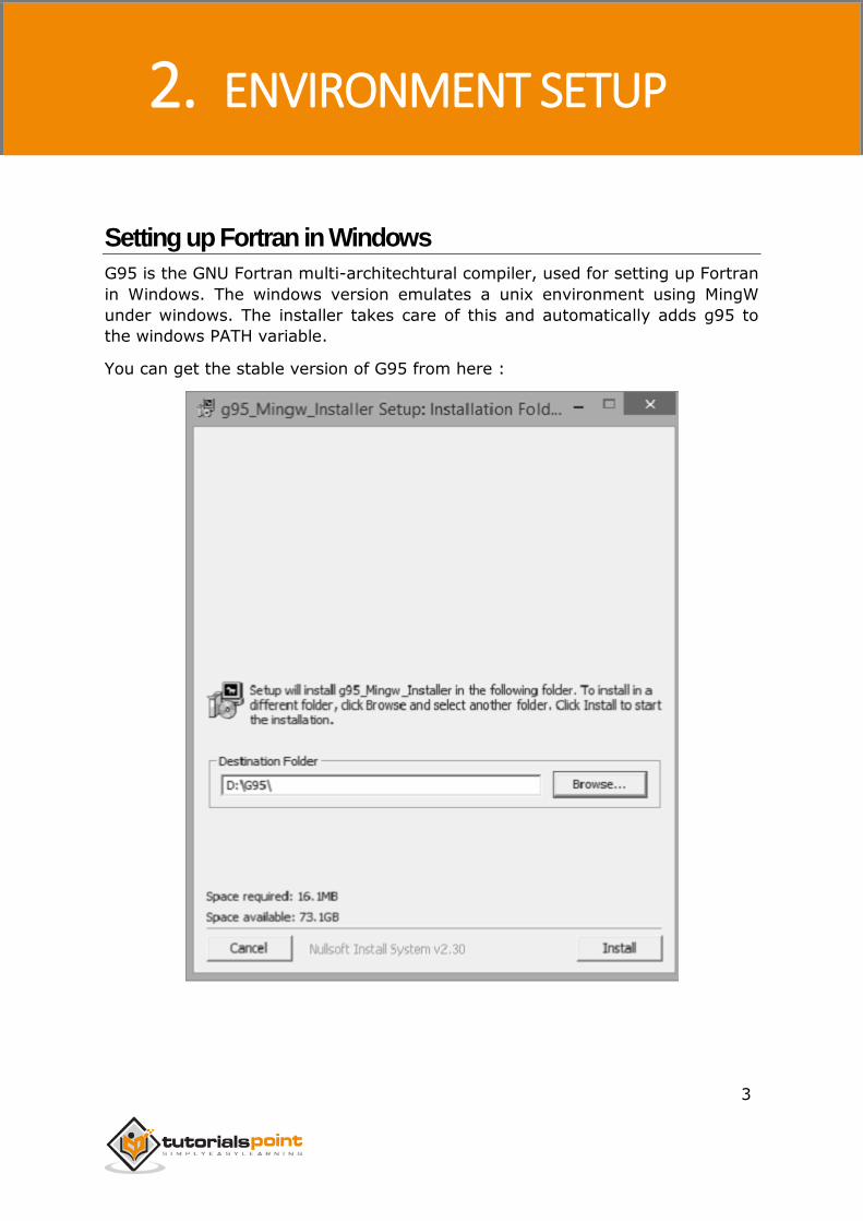
Setting up Fortran in Windows
G95 is the GNU Fortran multi-architechtural compiler, used for setting up Fortran
in Windows. The windows version emulates a unix environment using MingW
under windows. The installer takes care of this and automatically adds g95 to
the windows PATH variable.
You can get the stable version of G95 from here :
2. ENVIRONMENT SETUP
Fortran
4
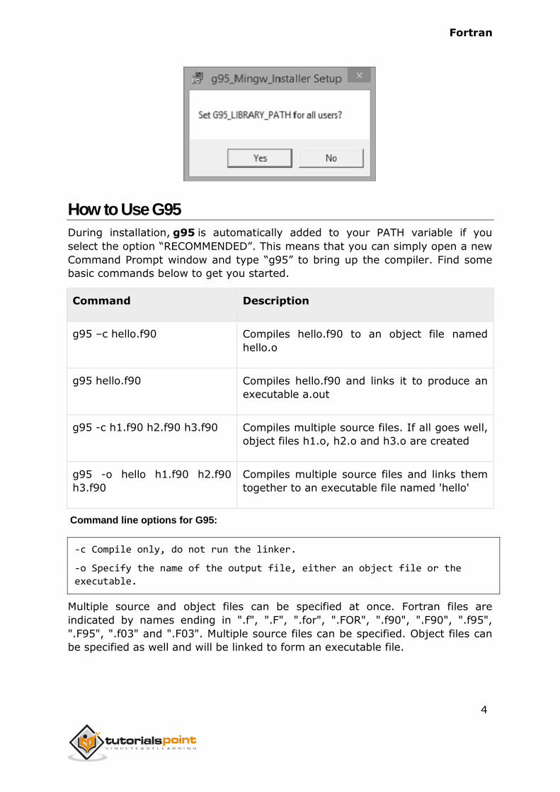
How to Use G95
During installation, g95 is automatically added to your PATH variable if you
select the option “RECOMMENDED”. This means that you can simply open a new
Command Prompt window and type “g95” to bring up the compiler. Find some
basic commands below to get you started.
Command Description
g95 –c hello.f90 Compiles hello.f90 to an object file named
hello.o
g95 hello.f90 Compiles hello.f90 and links it to produce an
executable a.out
g95 -c h1.f90 h2.f90 h3.f90 Compiles multiple source files. If all goes well,
object files h1.o, h2.o and h3.o are created
g95 -o hello h1.f90 h2.f90
h3.f90
Compiles multiple source files and links them
together to an executable file named 'hello'
Command line options for G95:
-c Compile only, do not run the linker.
-o Specify the name of the output file, either an object file or the
executable.
Multiple source and object files can be specified at once. Fortran files are
indicated by names ending in ".f", ".F", ".for", ".FOR", ".f90", ".F90", ".f95",
".F95", ".f03" and ".F03". Multiple source files can be specified. Object files can
be specified as well and will be linked to form an executable file.
Fortran
5
A Fortran program is made of a collection of program units like a main program,
modules, and external subprograms or procedures.
Each program contains one main program and may or may not contain other
program units. The syntax of the main program is as follows:
program program_name
implicit none
! type declaration statements
! executable statements
end program program_name
A Simple Program in Fortran
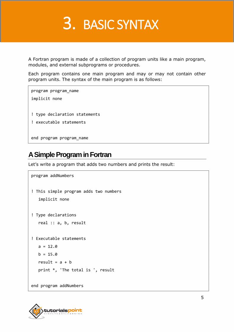
Let’s write a program that adds two numbers and prints the result:
program addNumbers
! This simple program adds two numbers
implicit none
! Type declarations
real :: a, b, result
! Executable statements
a = 12.0
b = 15.0
result = a + b
print *, 'The total is ', result
end program addNumbers
3. BASIC SYNTAX
Fortran
6
When you compile and execute the above program, it produces the following
result:
The total is 27.0000000
Please note that:
All Fortran programs start with the keyword program and end with the
keywordend program, followed by the name of the program.
The implicit none statement allows the compiler to check that all your
variable types are declared properly. You must always use implicit
none at the start of every program.
Comments in Fortran are started with the exclamation mark (!), as all
characters after this (except in a character string) are ignored by the
compiler.
The print * command displays data on the screen.
Indentation of code lines is a good practice for keeping a program
readable.
Fortran allows both uppercase and lowercase letters. Fortran is case-
insensitive, except for string literals.
Basics
The basic character set of Fortran contains:
the letters A ... Z and a ... z
the digits 0 ... 9
the underscore (_) character
the special characters = : + blank - * / ( ) [ ] , . $ ' ! " % & ; < > ?
Tokens are made of characters in the basic character set. A token could be a
keyword, an identifier, a constant, a string literal, or a symbol.
Program statements are made of tokens.
Identifier
An identifier is a name used to identify a variable, procedure, or any other user-
defined item. A name in Fortran must follow the following rules:
It cannot be longer than 31 characters.
It must be composed of alphanumeric characters (all the letters of the
alphabet, and the digits 0 to 9) and underscores (_).
Fortran
7
First character of a name must be a letter.
Names are case-insensitive
Keywords
Keywords are special words, reserved for the language. These reserved words
cannot be used as identifiers or names.
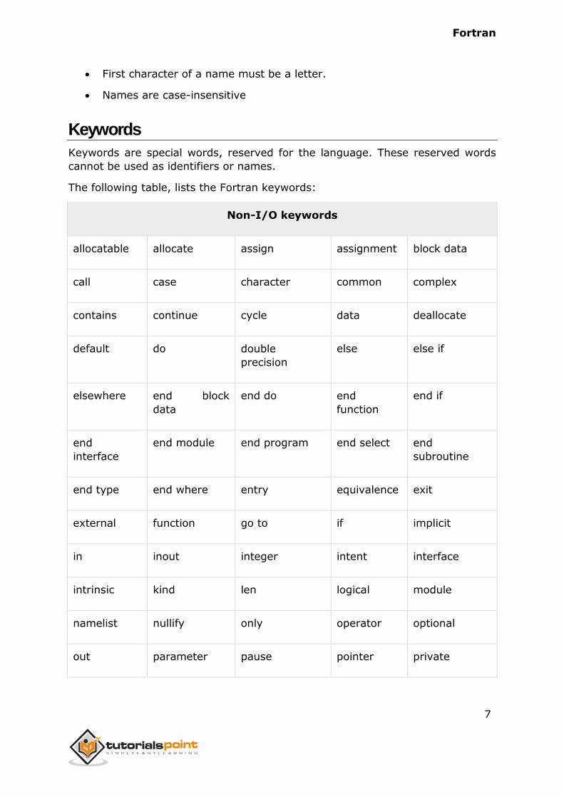
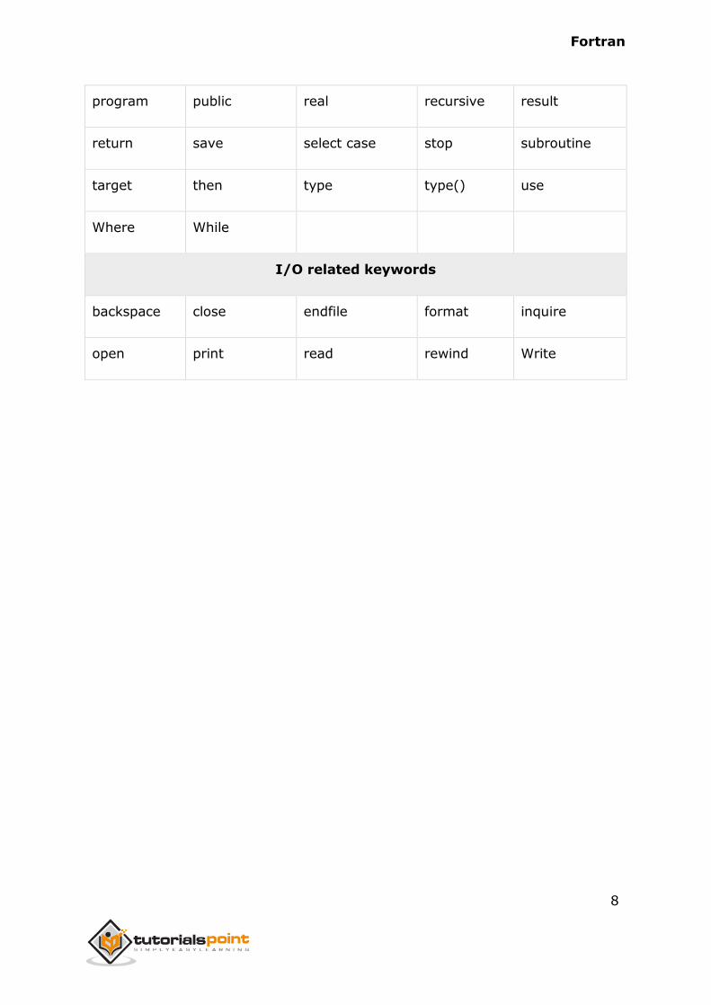
The following table, lists the Fortran keywords:
Non-I/O keywords
allocatable allocate assign assignment block data
call case character common complex
contains continue cycle data deallocate
default do double
precision
else else if
elsewhere end block
data
end do end
function
end if
end
interface
end module end program end select end
subroutine
end type end where entry equivalence exit
external function go to if implicit
in inout integer intent interface
intrinsic kind len logical module
namelist nullify only operator optional
out parameter pause pointer private
Fortran
8
program public real recursive result
return save select case stop subroutine
target then type type() use
Where While
I/O related keywords
backspace close endfile format inquire
open print read rewind Write
Fortran
9
Fortran provides five intrinsic data types, however, you can derive your own
data types as well. The five intrinsic types are:
Integer type
Real type
Complex type
Logical type
Character type
Integer Type
The integer types can hold only integer values. The following example extracts
the largest value that can be held in a usual four byte integer:
program testingInt
implicit none
integer :: largeval
print *, huge(largeval)
end program testingInt
When you compile and execute the above program it produces the following
result:
2147483647
Note that the huge() function gives the largest number that can be held by the
specific integer data type. You can also specify the number of bytes using
the kind specifier. The following example demonstrates this:
program testingInt
implicit none
!two byte integer
integer(kind=2) :: shortval
4. DATA TYPES
Fortran
10
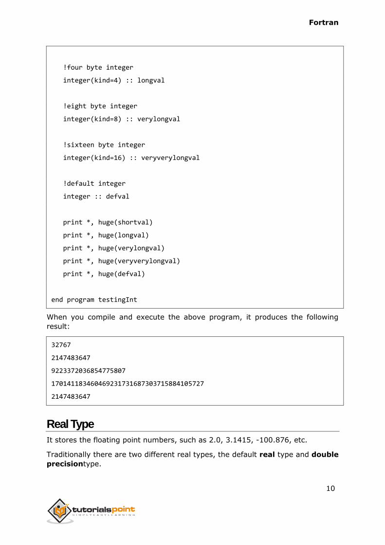
!four byte integer
integer(kind=4) :: longval
!eight byte integer
integer(kind=8) :: verylongval
!sixteen byte integer
integer(kind=16) :: veryverylongval
!default integer
integer :: defval
print *, huge(shortval)
print *, huge(longval)
print *, huge(verylongval)
print *, huge(veryverylongval)
print *, huge(defval)
end program testingInt
When you compile and execute the above program, it produces the following
result:
32767
2147483647
9223372036854775807
170141183460469231731687303715884105727
2147483647
Real Type
It stores the floating point numbers, such as 2.0, 3.1415, -100.876, etc.
Traditionally there are two different real types, the default real type and double
precisiontype.
Fortran
11
However, Fortran 90/95 provides more control over the precision of real and
integer data types through thekindspecifier, which we will study in the chapter
on Numbers.
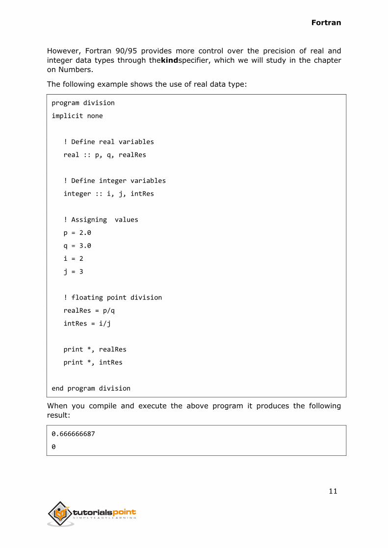
The following example shows the use of real data type:
program division
implicit none
! Define real variables
real :: p, q, realRes
! Define integer variables
integer :: i, j, intRes
! Assigning values
p = 2.0
q = 3.0
i = 2
j = 3
! floating point division
realRes = p/q
intRes = i/j
print *, realRes
print *, intRes
end program division
When you compile and execute the above program it produces the following
result:
0.666666687
0
Fortran
12
Complex Type
This is used for storing complex numbers. A complex number has two parts, the
real part and the imaginary part. Two consecutive numeric storage units store
these two parts.
For example, the complex number (3.0, -5.0) is equal to 3.0 – 5.0i
We will discuss Complex types in more detail, in the Numbers chapter.
Logical Type
There are only two logical values: .true. and .false.
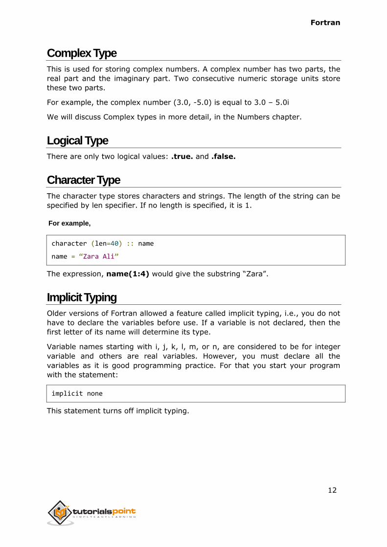
Character Type
The character type stores characters and strings. The length of the string can be
specified by len specifier. If no length is specified, it is 1.
For example,
character (len=40) :: name
name = “Zara Ali”
The expression, name(1:4) would give the substring “Zara”.
Implicit Typing
Older versions of Fortran allowed a feature called implicit typing, i.e., you do not
have to declare the variables before use. If a variable is not declared, then the
first letter of its name will determine its type.
Variable names starting with i, j, k, l, m, or n, are considered to be for integer
variable and others are real variables. However, you must declare all the
variables as it is good programming practice. For that you start your program
with the statement:
implicit none
This statement turns off implicit typing.
Fortran
13
A variable is nothing but a name given to a storage area that our programs can
manipulate. Each variable should have a specific type, which determines the size
and layout of the variable's memory; the range of values that can be stored
within that memory; and the set of operations that can be applied to the
variable.
The name of a variable can be composed of letters, digits, and the underscore
character. A name in Fortran must follow the following rules:
It cannot be longer than 31 characters.
It must be composed of alphanumeric characters (all the letters of the
alphabet, and the digits 0 to 9) and underscores (_).
First character of a name must be a letter.
Names are case-insensitive.
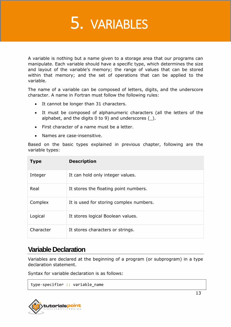
Based on the basic types explained in previous chapter, following are the
variable types:
Type Description
Integer It can hold only integer values.
Real It stores the floating point numbers.
Complex It is used for storing complex numbers.
Logical It stores logical Boolean values.
Character It stores characters or strings.
Variable Declaration
Variables are declared at the beginning of a program (or subprogram) in a type
declaration statement.
Syntax for variable declaration is as follows:
type-specifier :: variable_name
5. VARIABLES
Fortran
14
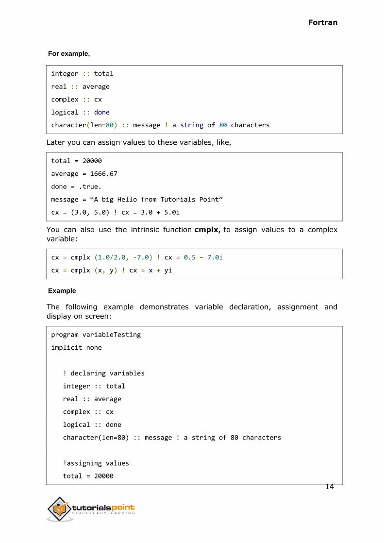
For example,
integer :: total
real :: average
complex :: cx
logical :: done
character(len=80) :: message ! a string of 80 characters
Later you can assign values to these variables, like,
total = 20000
average = 1666.67
done = .true.
message = “A big Hello from Tutorials Point”
cx = (3.0, 5.0) ! cx = 3.0 + 5.0i
You can also use the intrinsic function cmplx, to assign values to a complex
variable:
cx = cmplx (1.0/2.0, -7.0) ! cx = 0.5 – 7.0i
cx = cmplx (x, y) ! cx = x + yi
Example
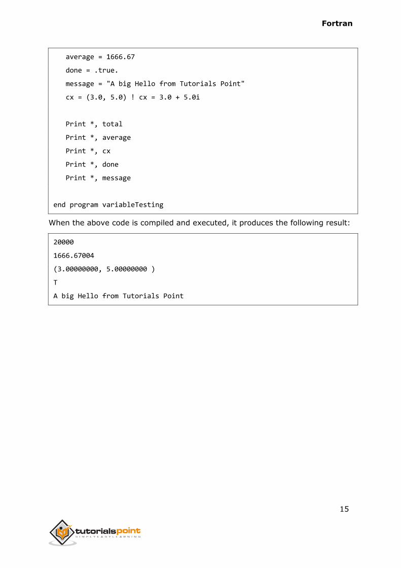
The following example demonstrates variable declaration, assignment and
display on screen:
program variableTesting
implicit none
! declaring variables
integer :: total
real :: average
complex :: cx
logical :: done
character(len=80) :: message ! a string of 80 characters
!assigning values
total = 20000
Fortran
15
average = 1666.67
done = .true.
message = "A big Hello from Tutorials Point"
cx = (3.0, 5.0) ! cx = 3.0 + 5.0i
Print *, total
Print *, average
Print *, cx
Print *, done
Print *, message
end program variableTesting
When the above code is compiled and executed, it produces the following result:
20000
1666.67004
(3.00000000, 5.00000000 )
T
A big Hello from Tutorials Point
Fortran
16
The constants refer to the fixed values that the program cannot alter during its
execution. These fixed values are also called literals.
Constants can be of any of the basic data types like an integer constant, a
floating constant, a character constant, a complex constant, or a string literal.
There are only two logical constants : .true. and .false.
The constants are treated just like regular variables, except that their values
cannot be modified after their definition.
Named Constants and Literals
There are two types of constants:
Literal constants
Named constants
A literal constant have a value, but no name.
For example, following are the literal constants:
Type Example
Integer constants 0 1 -1 300 123456789
Real constants 0.0 1.0 -1.0 123.456 7.1E+10 -52.715E-30
Complex constants (0.0, 0.0) (-123.456E+30, 987.654E-29)
Logical constants .true. .false.
Character constants "PQR" "a" "123'abc$%#@!"
" a quote "" "
'PQR' 'a' '123"abc$%#@!'
' an apostrophe '' '
A named constant has a value as well as a name.
6. CONSTANTS
Fortran
17
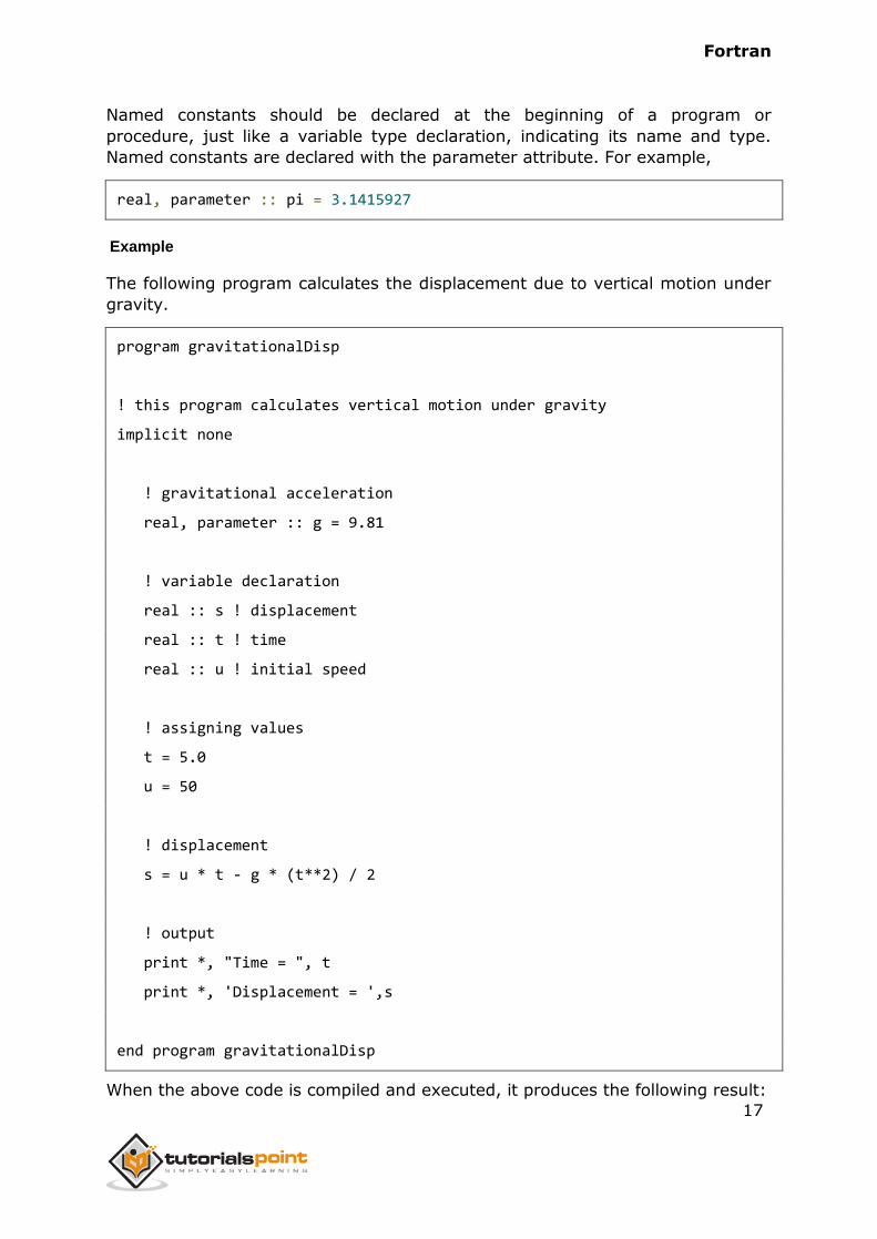
Named constants should be declared at the beginning of a program or
procedure, just like a variable type declaration, indicating its name and type.
Named constants are declared with the parameter attribute. For example,
real, parameter :: pi = 3.1415927
Example
The following program calculates the displacement due to vertical motion under
gravity.
program gravitationalDisp
! this program calculates vertical motion under gravity
implicit none
! gravitational acceleration
real, parameter :: g = 9.81
! variable declaration
real :: s ! displacement
real :: t ! time
real :: u ! initial speed
! assigning values
t = 5.0
u = 50
! displacement
s = u * t - g * (t**2) / 2
! output
print *, "Time = ", t
print *, 'Displacement = ',s
end program gravitationalDisp
When the above code is compiled and executed, it produces the following result:

Fortran
18
Time = 5.00000000
Displacement = 127.374992
Fortran
19
An operator is a symbol that tells the compiler to perform specific mathematical
or logical manipulations. Fortran provides the following types of operators:
Arithmetic Operators
Relational Operators
Logical Operators
Let us look at all these types of operators one by one.
Arithmetic Operators
Following table shows all the arithmetic operators supported by Fortran. Assume
variable Aholds 5 and variable B holds 3 then:
Operator Description Example
+ Addition Operator, adds two operands. A + B will give 8
- Subtraction Operator, subtracts second
operand from the first.
A - B will give 2
* Multiplication Operator, multiplies both
operands.
A * B will give 15
/ Division Operator, divides numerator by de-
numerator.
A / B will give 1
** Exponentiation Operator, raises one operand
to the power of the other.
A ** B will give
125
Example
Try the following example to understand all the arithmetic operators available in
Fortran:
program arithmeticOp
! this program performs arithmetic calculation
7. OPERATORS
Fortran
20
implicit none
! variable declaration
integer :: a, b, c
! assigning values
a = 5
b = 3
! Exponentiation
c = a ** b
! output
print *, "c = ", c
! Multiplication
c = a * b
! output
print *, "c = ", c
! Division
c = a / b
! output
print *, "c = ", c
! Addition
c = a + b
! output
print *, "c = ", c
Fortran
21
! Subtraction
c = a - b
! output
print *, "c = ", c
end program arithmeticOp
When you compile and execute the above program, it produces the following
result:
c = 125
c = 15
c = 1
c = 8
c = 2
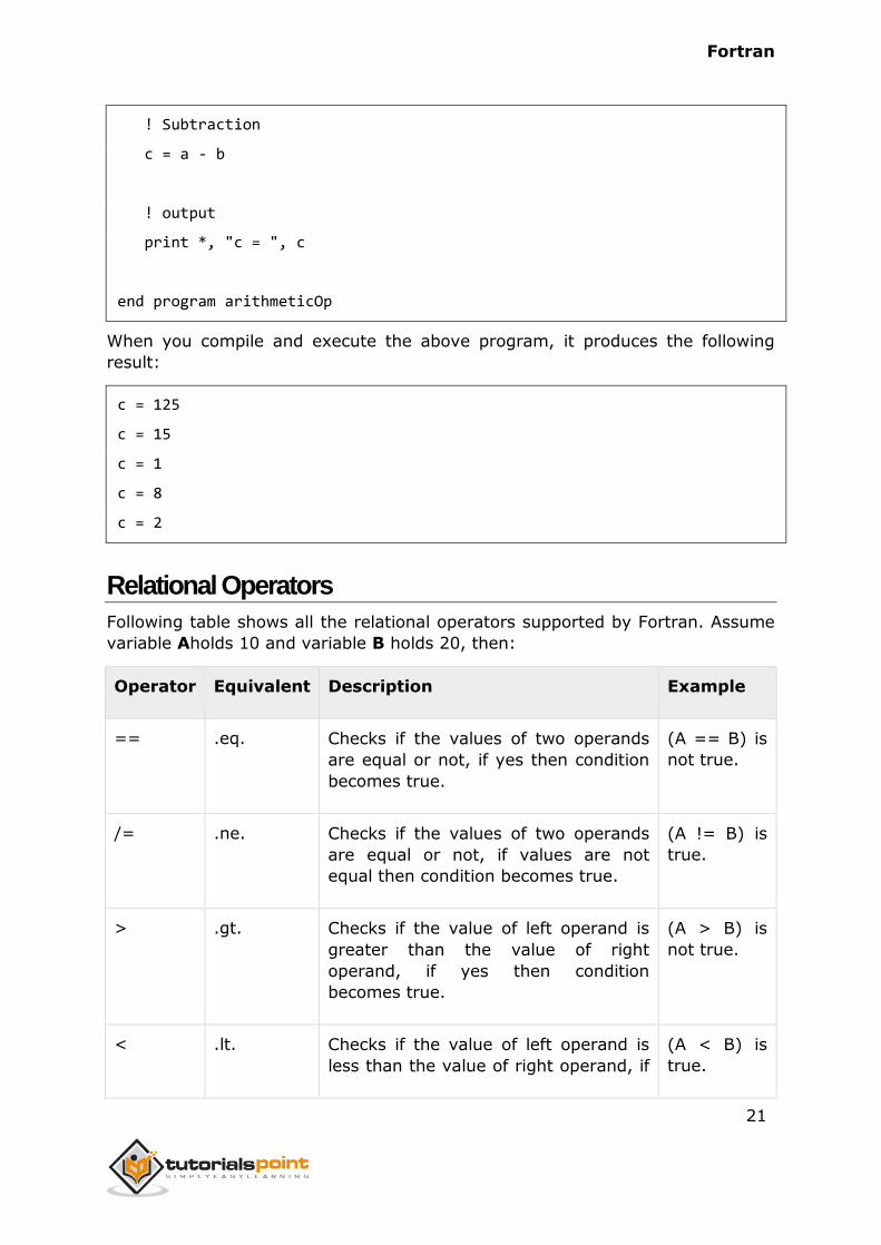
Relational Operators
Following table shows all the relational operators supported by Fortran. Assume
variable Aholds 10 and variable B holds 20, then:
Operator Equivalent Description Example
== .eq. Checks if the values of two operands
are equal or not, if yes then condition
becomes true.
(A == B) is
not true.
/= .ne. Checks if the values of two operands
are equal or not, if values are not
equal then condition becomes true.
(A != B) is
true.
> .gt. Checks if the value of left operand is
greater than the value of right
operand, if yes then condition
becomes true.
(A > B) is
not true.
< .lt. Checks if the value of left operand is
less than the value of right operand, if
(A < B) is
true.
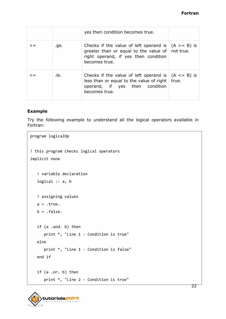
Fortran
22
yes then condition becomes true.
>= .ge. Checks if the value of left operand is
greater than or equal to the value of
right operand, if yes then condition
becomes true.
(A >= B) is
not true.
<= .le. Checks if the value of left operand is
less than or equal to the value of right
operand, if yes then condition
becomes true.
(A <= B) is
true.
Example
Try the following example to understand all the logical operators available in
Fortran:
program logicalOp
! this program checks logical operators
implicit none
! variable declaration
logical :: a, b
! assigning values
a = .true.
b = .false.
if (a .and. b) then
print *, "Line 1 - Condition is true"
else
print *, "Line 1 - Condition is false"
end if
if (a .or. b) then
print *, "Line 2 - Condition is true"
Fortran
23
else
print *, "Line 2 - Condition is false"
end if
! changing values
a = .false.
b = .true.
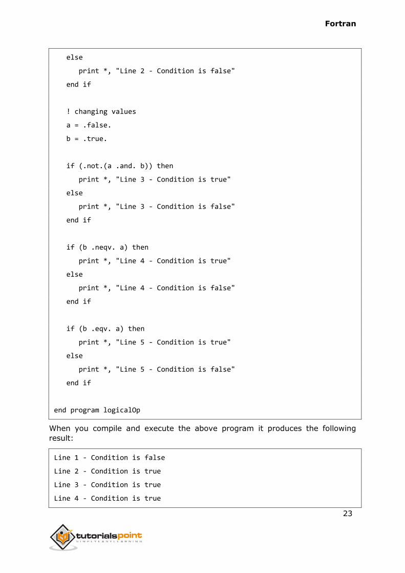
if (.not.(a .and. b)) then
print *, "Line 3 - Condition is true"
else
print *, "Line 3 - Condition is false"
end if
if (b .neqv. a) then
print *, "Line 4 - Condition is true"
else
print *, "Line 4 - Condition is false"
end if
if (b .eqv. a) then
print *, "Line 5 - Condition is true"
else
print *, "Line 5 - Condition is false"
end if
end program logicalOp
When you compile and execute the above program it produces the following
result:
Line 1 - Condition is false
Line 2 - Condition is true
Line 3 - Condition is true
Line 4 - Condition is true
Fortran
24
Line 5 - Condition is false
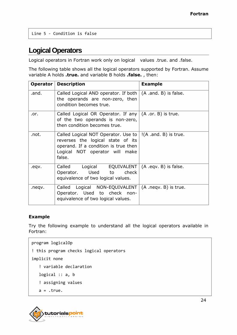
Logical Operators
Logical operators in Fortran work only on logical values .true. and .false.
The following table shows all the logical operators supported by Fortran. Assume
variable A holds .true. and variable B holds .false. , then:
Operator Description Example
.and. Called Logical AND operator. If both
the operands are non-zero, then
condition becomes true.
(A .and. B) is false.
.or. Called Logical OR Operator. If any
of the two operands is non-zero,
then condition becomes true.
(A .or. B) is true.
.not. Called Logical NOT Operator. Use to
reverses the logical state of its
operand. If a condition is true then
Logical NOT operator will make
false.
!(A .and. B) is true.
.eqv. Called Logical EQUIVALENT
Operator. Used to check
equivalence of two logical values.
(A .eqv. B) is false.
.neqv. Called Logical NON-EQUIVALENT
Operator. Used to check non-
equivalence of two logical values.
(A .neqv. B) is true.
Example
Try the following example to understand all the logical operators available in
Fortran:
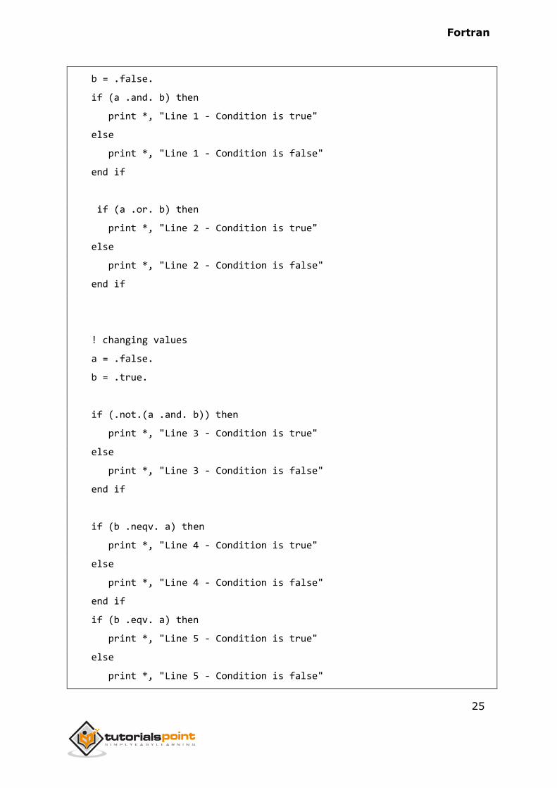
program logicalOp
! this program checks logical operators
implicit none
! variable declaration
logical :: a, b
! assigning values
a = .true.
Fortran
25
b = .false.
if (a .and. b) then
print *, "Line 1 - Condition is true"
else
print *, "Line 1 - Condition is false"
end if
if (a .or. b) then
print *, "Line 2 - Condition is true"
else
print *, "Line 2 - Condition is false"
end if
! changing values
a = .false.
b = .true.
if (.not.(a .and. b)) then
print *, "Line 3 - Condition is true"
else
print *, "Line 3 - Condition is false"
end if
if (b .neqv. a) then
print *, "Line 4 - Condition is true"
else
print *, "Line 4 - Condition is false"
end if
if (b .eqv. a) then
print *, "Line 5 - Condition is true"
else
print *, "Line 5 - Condition is false"
Fortran
26
end if
end program logicalOp
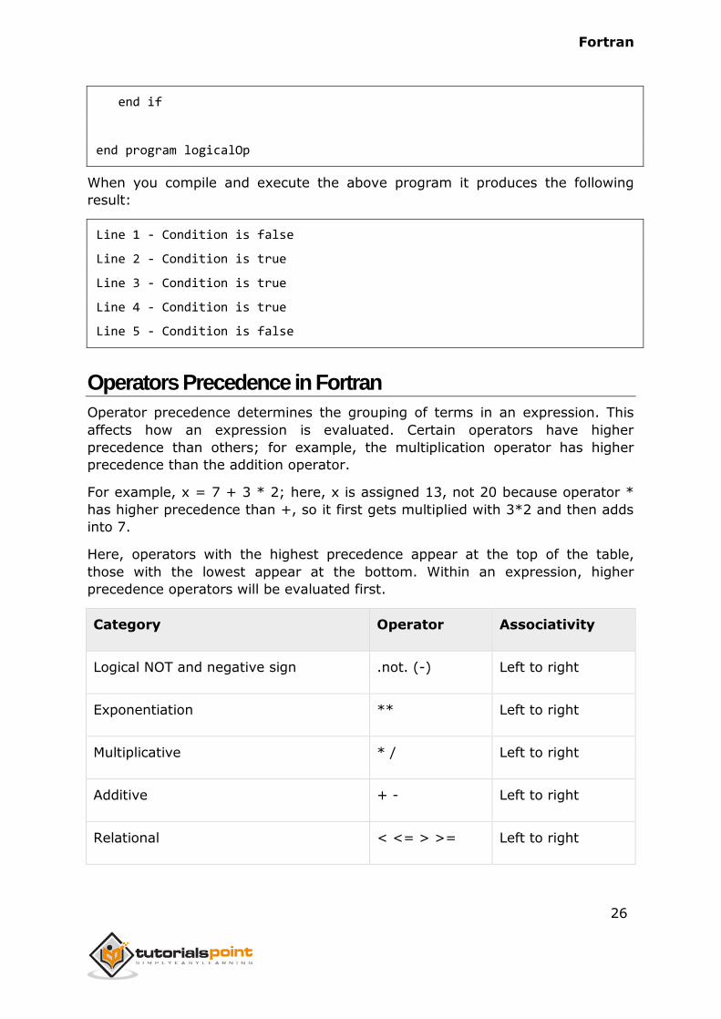
When you compile and execute the above program it produces the following
result:
Line 1 - Condition is false
Line 2 - Condition is true
Line 3 - Condition is true
Line 4 - Condition is true
Line 5 - Condition is false
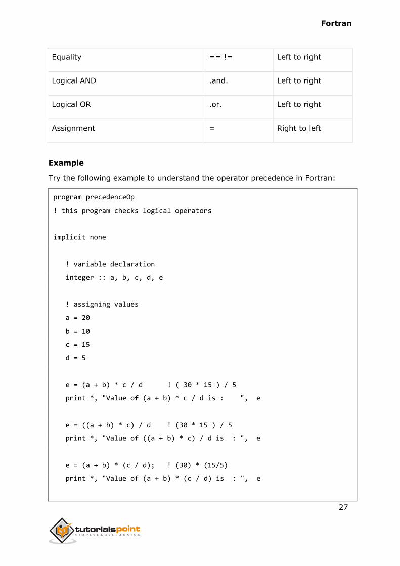
Operators Precedence in Fortran
Operator precedence determines the grouping of terms in an expression. This
affects how an expression is evaluated. Certain operators have higher
precedence than others; for example, the multiplication operator has higher
precedence than the addition operator.
For example, x = 7 + 3 * 2; here, x is assigned 13, not 20 because operator *
has higher precedence than +, so it first gets multiplied with 3*2 and then adds
into 7.
Here, operators with the highest precedence appear at the top of the table,
those with the lowest appear at the bottom. Within an expression, higher
precedence operators will be evaluated first.
Category Operator Associativity
Logical NOT and negative sign .not. (-) Left to right
Exponentiation ** Left to right
Multiplicative * / Left to right
Additive + - Left to right
Relational < <= > >= Left to right
Fortran
27
Equality == != Left to right
Logical AND .and. Left to right
Logical OR .or. Left to right
Assignment = Right to left
Example
Try the following example to understand the operator precedence in Fortran:
program precedenceOp
! this program checks logical operators
implicit none
! variable declaration
integer :: a, b, c, d, e
! assigning values
a = 20
b = 10
c = 15
d = 5
e = (a + b) * c / d ! ( 30 * 15 ) / 5
print *, "Value of (a + b) * c / d is : ", e
e = ((a + b) * c) / d ! (30 * 15 ) / 5
print *, "Value of ((a + b) * c) / d is : ", e
e = (a + b) * (c / d); ! (30) * (15/5)
print *, "Value of (a + b) * (c / d) is : ", e
Fortran
28
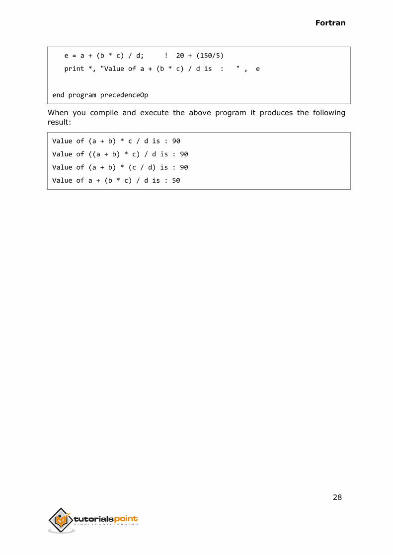
e = a + (b * c) / d; ! 20 + (150/5)
print *, "Value of a + (b * c) / d is : " , e
end program precedenceOp
When you compile and execute the above program it produces the following
result:
Value of (a + b) * c / d is : 90
Value of ((a + b) * c) / d is : 90
Value of (a + b) * (c / d) is : 90
Value of a + (b * c) / d is : 50
Fortran
29
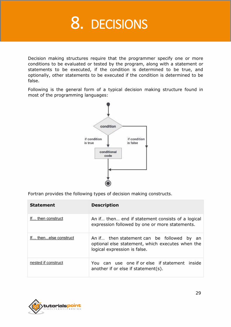
Decision making structures require that the programmer specify one or more
conditions to be evaluated or tested by the program, along with a statement or
statements to be executed, if the condition is determined to be true, and
optionally, other statements to be executed if the condition is determined to be
false.
Following is the general form of a typical decision making structure found in
most of the programming languages:
Fortran provides the following types of decision making constructs.
Statement Description
If… then construct An if… then… end if statement consists of a logical
expression followed by one or more statements.
If… then...else construct An if… then statement can be followed by an
optional else statement, which executes when the
logical expression is false.
nested if construct You can use one if or else if statement inside
another if or else if statement(s).
8. DECISIONS
Fortran
30
select case construct A select case statement allows a variable to be
tested for equality against a list of values.
nested select case construct You can use one select case statement inside
another select case statement(s).
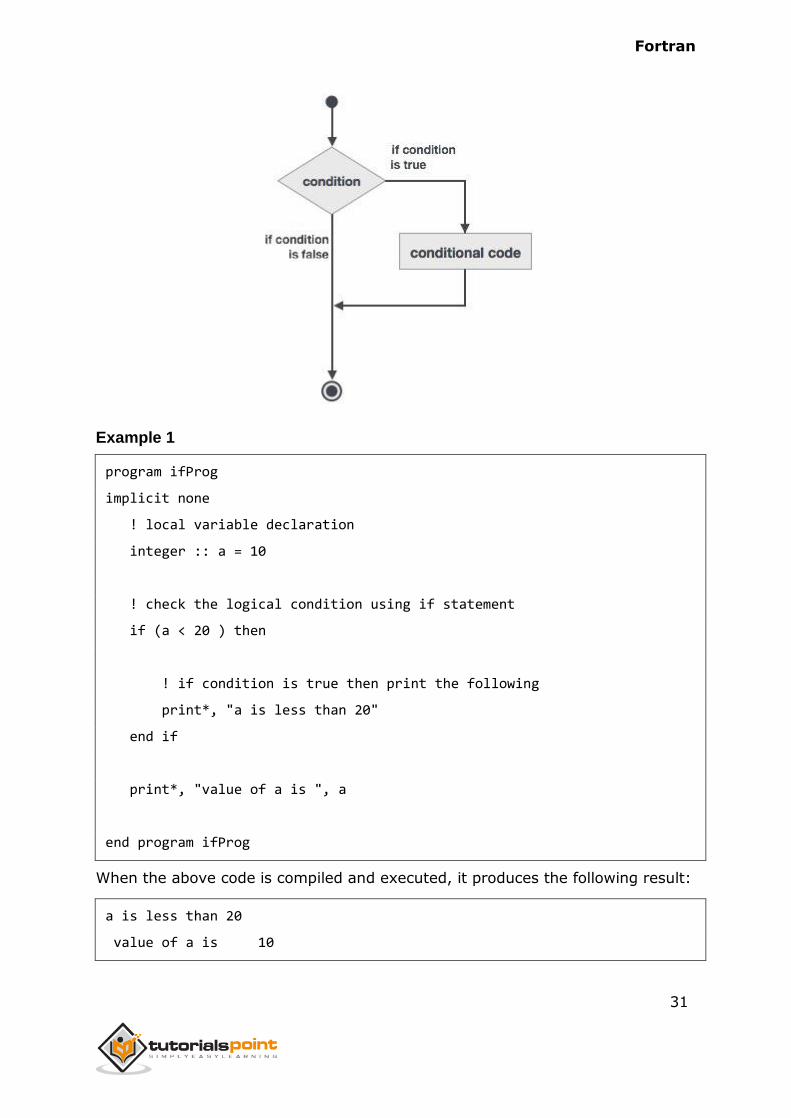
If…then Construct
An if… then statement consists of a logical expression followed by one or more
statements and terminated by an end if statement.
Syntax
The basic syntax of an if… then statement is:
if (logical expression) then
statement
end if
However, you can give a name to the if block, then the syntax of the named if
statement would be, like:
[name:] if (logical expression) then
! various statements
. . .
end if [name]
If the logical expression evaluates to true, then the block of code inside the
if…then statement will be executed. If logical expression evaluates to false,
then the first set of code after the end if statement will be executed.
Flow Diagram
Fortran
31
Example 1
program ifProg
implicit none
! local variable declaration
integer :: a = 10
! check the logical condition using if statement
if (a < 20 ) then
! if condition is true then print the following
print*, "a is less than 20"
end if
print*, "value of a is ", a
end program ifProg
When the above code is compiled and executed, it produces the following result:
a is less than 20
value of a is 10
Fortran
32
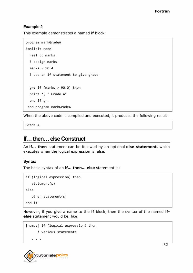
Example 2
This example demonstrates a named if block:
program markGradeA
implicit none
real :: marks
! assign marks
marks = 90.4
! use an if statement to give grade
gr: if (marks > 90.0) then
print *, " Grade A"
end if gr
end program markGradeA
When the above code is compiled and executed, it produces the following result:
Grade A
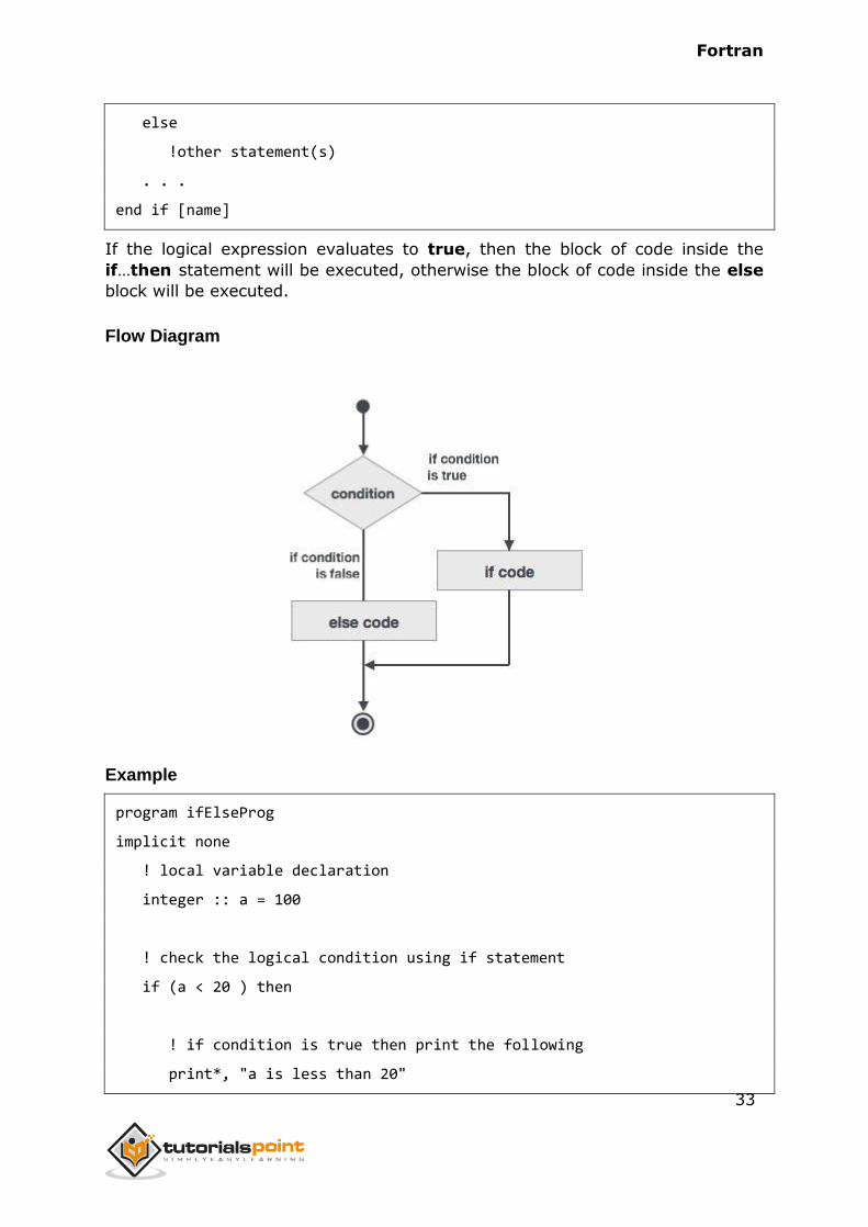
If… then… else Construct
An if… then statement can be followed by an optional else statement, which
executes when the logical expression is false.
Syntax
The basic syntax of an if… then… else statement is:
if (logical expression) then
statement(s)
else
other_statement(s)
end if
However, if you give a name to the if block, then the syntax of the named if-
else statement would be, like:
[name:] if (logical expression) then
! various statements
. . .
Fortran
33
else
!other statement(s)
. . .
end if [name]
If the logical expression evaluates to true, then the block of code inside the
if…then statement will be executed, otherwise the block of code inside the else
block will be executed.
Flow Diagram
Example
program ifElseProg
implicit none
! local variable declaration
integer :: a = 100
! check the logical condition using if statement
if (a < 20 ) then
! if condition is true then print the following
print*, "a is less than 20"
Fortran
34
else
print*, "a is not less than 20"
end if
print*, "value of a is ", a
end program ifElseProg
When the above code is compiled and executed, it produces the following result:
a is not less than 20
value of a is 100
if...else if...else Statement
An if statement construct can have one or more optional else-if constructs.
When the ifcondition fails, the immediately followed else-if is executed. When
the else-if also fails, its successor else-if statement (if any) is executed, and so
on.
The optional else is placed at the end and it is executed when none of the above
conditions hold true.
All else statements (else-if and else) are optional.
else-if can be used one or more times
else must always be placed at the end of construct and should appear
only once.
Syntax
The syntax of an if...else if...else statement is:
[name:]
if (logical expression 1) then
! block 1
else if (logical expression 2) then
! block 2
else if (logical expression 3) then
! block 3
else
Fortran
35
! block 4
end if [name]
Example
program ifElseIfElseProg
implicit none
! local variable declaration
integer :: a = 100
! check the logical condition using if statement
if( a == 10 ) then
! if condition is true then print the following
print*, "Value of a is 10"
else if( a == 20 ) then
! if else if condition is true
print*, "Value of a is 20"
else if( a == 30 ) then
! if else if condition is true
print*, "Value of a is 30"
else
! if none of the conditions is true
print*, "None of the values is matching"
end if
Fortran
36
print*, "exact value of a is ", a
end program ifElseIfElseProg
When the above code is compiled and executed, it produces the following result:
None of the values is matching
exact value of a is 100
Nested If Construct
You can use one if or else if statement inside another if or else if statement(s).
Syntax
The syntax for a nested if statement is as follows:
if ( logical_expression 1) then
!Executes when the boolean expression 1 is true
…
if(logical_expression 2)then
! Executes when the boolean expression 2 is true
…
end if
end if
Example
program nestedIfProg
implicit none
! local variable declaration
integer :: a = 100, b= 200
! check the logical condition using if statement
if( a == 100 ) then
! if condition is true then check the following
Fortran
37
if( b == 200 ) then
! if inner if condition is true
print*, "Value of a is 100 and b is 200"
end if
end if
print*, "exact value of a is ", a
print*, "exact value of b is ", b
end program nestedIfProg
When the above code is compiled and executed, it produces the following result:
Value of a is 100 and b is 200
exact value of a is 100
exact value of b is 200
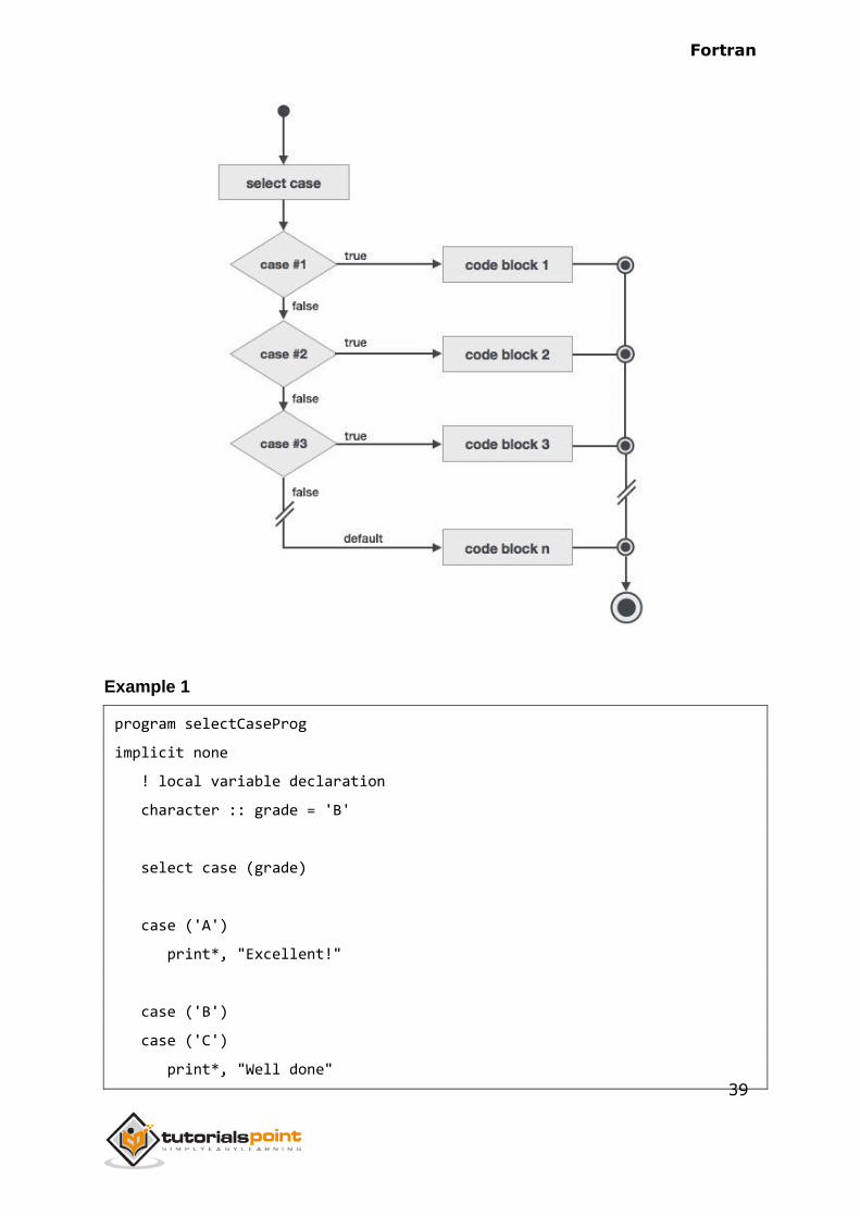
Select Case Construct
A select case statement allows a variable to be tested for equality against a list
of values. Each value is called a case, and the variable being selected on is
checked for each select case.
Syntax
The syntax for the select case construct is as follows:
[name:] select case (expression)
case (selector1)
! some statements
... case (selector2)
! other statements
...
case default
! more statements
...
Fortran
38
end select [name]
The following rules apply to a select statement:
The logical expression used in a select statement could be logical,
character, or integer (but not real) expression.
You can have any number of case statements within a select. Each case is
followed by the value to be compared to and could be logical, character,
or integer (but not real) expression and determines which statements are
executed.
The constant-expression for a case, must be the same data type as the
variable in the select, and it must be a constant or a literal.
When the variable being selected on, is equal to a case, the statements
following that case will execute until the next case statement is reached.
The case default block is executed if the expression in select case
(expression) does not match any of the selectors.
Flow Diagram
Fortran
39
Example 1
program selectCaseProg
implicit none
! local variable declaration
character :: grade = 'B'
select case (grade)
case ('A')
print*, "Excellent!"
case ('B')
case ('C')
print*, "Well done"
Fortran
40
case ('D')
print*, "You passed"
case ('F')
print*, "Better try again"
case default
print*, "Invalid grade"
end select
print*, "Your grade is ", grade
end program selectCaseProg
When the above code is compiled and executed, it produces the following result:
Your grade is B
Specifying a Range for the Selector
You can specify a range for the selector, by specifying a lower and upper limit
separated by a colon:
case (low:high)
The following example demonstrates this:
Example 2
program selectCaseProg
implicit none
! local variable declaration
integer :: marks = 78
select case (marks)
case (91:100)
print*, "Excellent!"
Fortran
41
case (81:90)
print*, "Very good!"
case (71:80)
print*, "Well done!"
case (61:70)
print*, "Not bad!"
case (41:60)
print*, "You passed!"
case (:40)
print*, "Better try again!"
case default
print*, "Invalid marks"
end select
print*, "Your marks is ", marks
end program selectCaseProg
When the above code is compiled and executed, it produces the following result:
Well done!
Your marks is 78
Fortran
42
Nested Select Case Construct
You can use one select case statement inside another select case
statement(s).
Syntax
select case(a)
case (100)
print*, "This is part of outer switch", a
select case(b)
case (200)
print*, "This is part of inner switch", a
end select
end select
Example
program nestedSelectCase
! local variable definition
integer :: a = 100
integer :: b = 200
select case(a)
case (100)
print*, "This is part of outer switch", a
select case(b)
case (200)
print*, "This is part of inner switch", a
end select
end select
print*, "Exact value of a is : ", a
print*, "Exact value of b is : ", b
end program nestedSelectCase

Fortran
43
When the above code is compiled and executed, it produces the following result:
This is part of outer switch 100
This is part of inner switch 100
Exact value of a is : 100
Exact value of b is : 200
Fortran
44
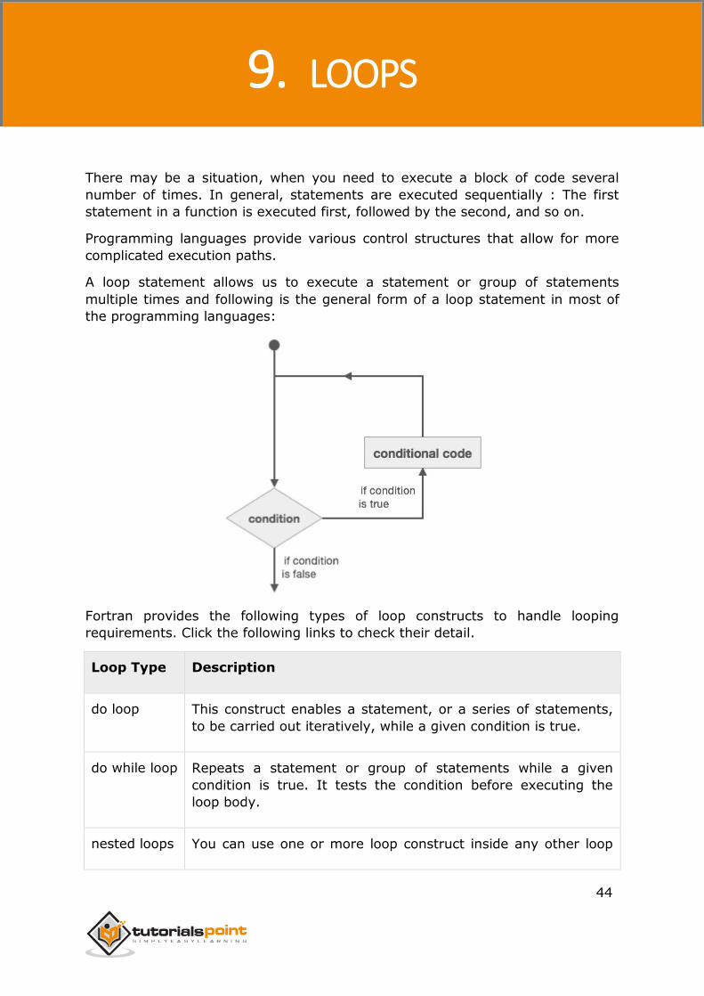
There may be a situation, when you need to execute a block of code several
number of times. In general, statements are executed sequentially : The first
statement in a function is executed first, followed by the second, and so on.
Programming languages provide various control structures that allow for more
complicated execution paths.
A loop statement allows us to execute a statement or group of statements
multiple times and following is the general form of a loop statement in most of
the programming languages:
Fortran provides the following types of loop constructs to handle looping
requirements. Click the following links to check their detail.
Loop Type Description
do loop This construct enables a statement, or a series of statements,
to be carried out iteratively, while a given condition is true.
do while loop Repeats a statement or group of statements while a given
condition is true. It tests the condition before executing the
loop body.
nested loops You can use one or more loop construct inside any other loop
9. LOOPS
Fortran
45
construct.
do Loop
The do loop construct enables a statement, or a series of statements, to be
carried out iteratively, while a given condition is true.
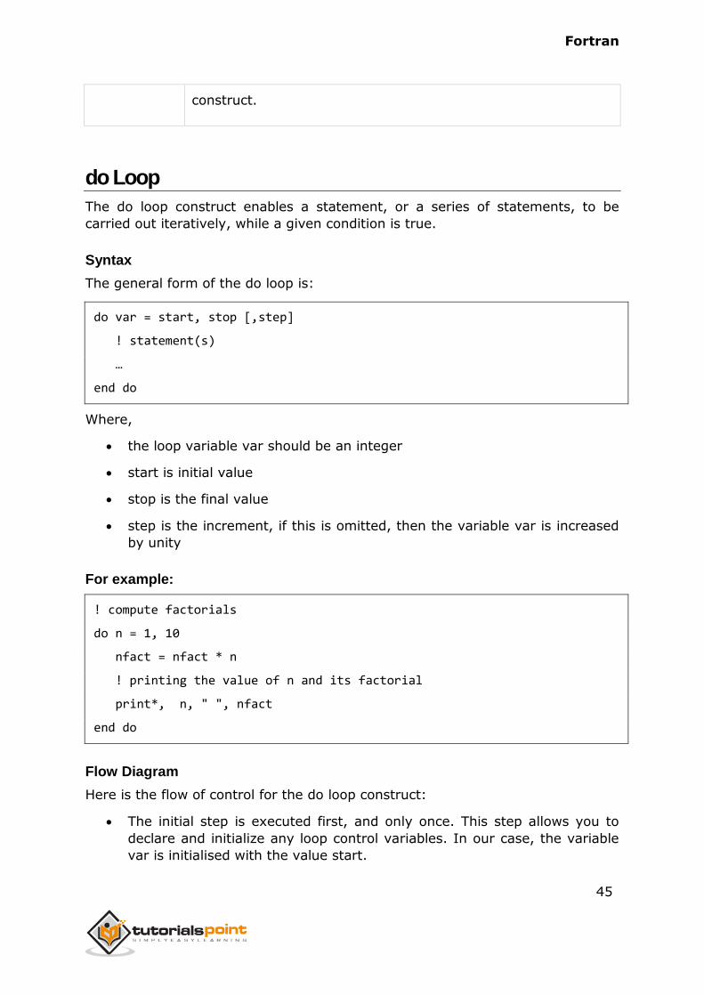
Syntax
The general form of the do loop is:
do var = start, stop [,step]
! statement(s)
…
end do
Where,
the loop variable var should be an integer
start is initial value
stop is the final value
step is the increment, if this is omitted, then the variable var is increased
by unity
For example:
! compute factorials
do n = 1, 10
nfact = nfact * n
! printing the value of n and its factorial
print*, n, " ", nfact
end do
Flow Diagram
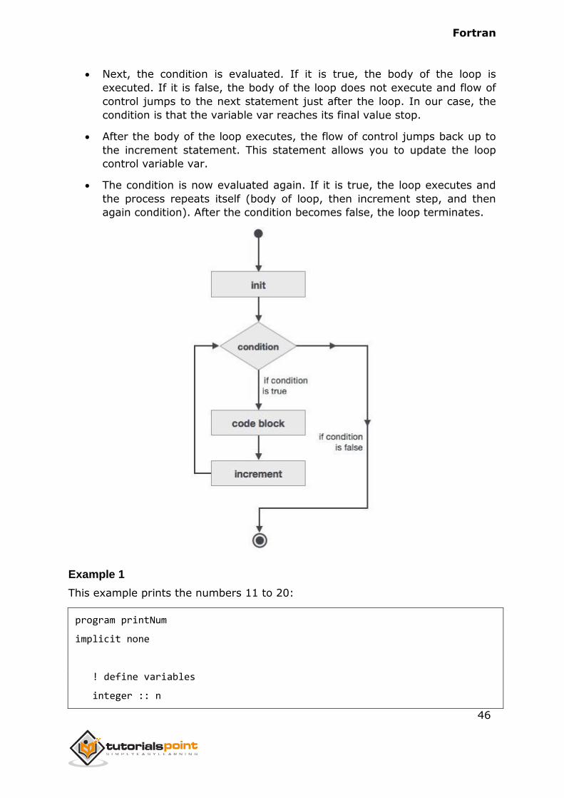
Here is the flow of control for the do loop construct:
The initial step is executed first, and only once. This step allows you to
declare and initialize any loop control variables. In our case, the variable
var is initialised with the value start.
Fortran
46
Next, the condition is evaluated. If it is true, the body of the loop is
executed. If it is false, the body of the loop does not execute and flow of
control jumps to the next statement just after the loop. In our case, the
condition is that the variable var reaches its final value stop.
After the body of the loop executes, the flow of control jumps back up to
the increment statement. This statement allows you to update the loop
control variable var.
The condition is now evaluated again. If it is true, the loop executes and
the process repeats itself (body of loop, then increment step, and then
again condition). After the condition becomes false, the loop terminates.
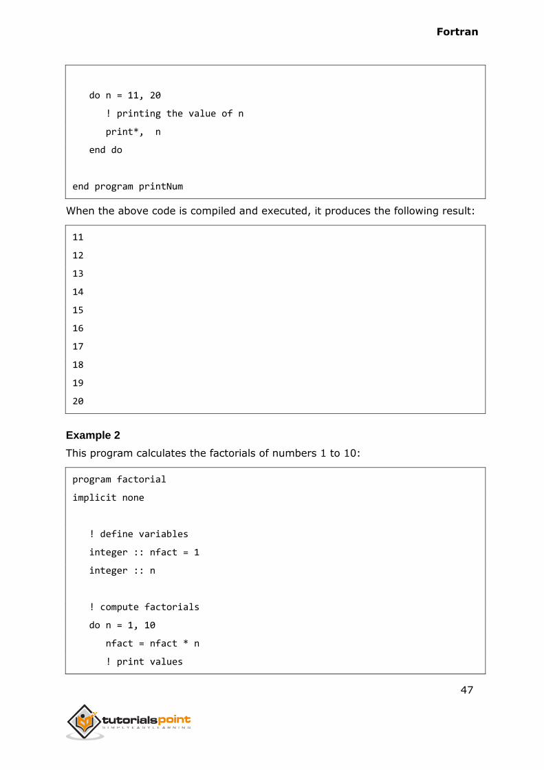
Example 1
This example prints the numbers 11 to 20:
program printNum
implicit none
! define variables
integer :: n
Fortran
47
do n = 11, 20
! printing the value of n
print*, n
end do
end program printNum
When the above code is compiled and executed, it produces the following result:
11
12
13
14
15
16
17
18
19
20
Example 2
This program calculates the factorials of numbers 1 to 10:
program factorial
implicit none
! define variables
integer :: nfact = 1
integer :: n
! compute factorials
do n = 1, 10
nfact = nfact * n
! print values
Fortran
48
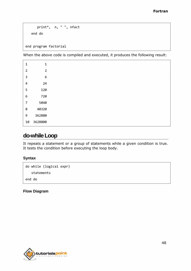
print*, n, " ", nfact
end do
end program factorial
When the above code is compiled and executed, it produces the following result:
1 1
2 2
3 6
4 24
5 120
6 720
7 5040
8 40320
9 362880
10 3628800
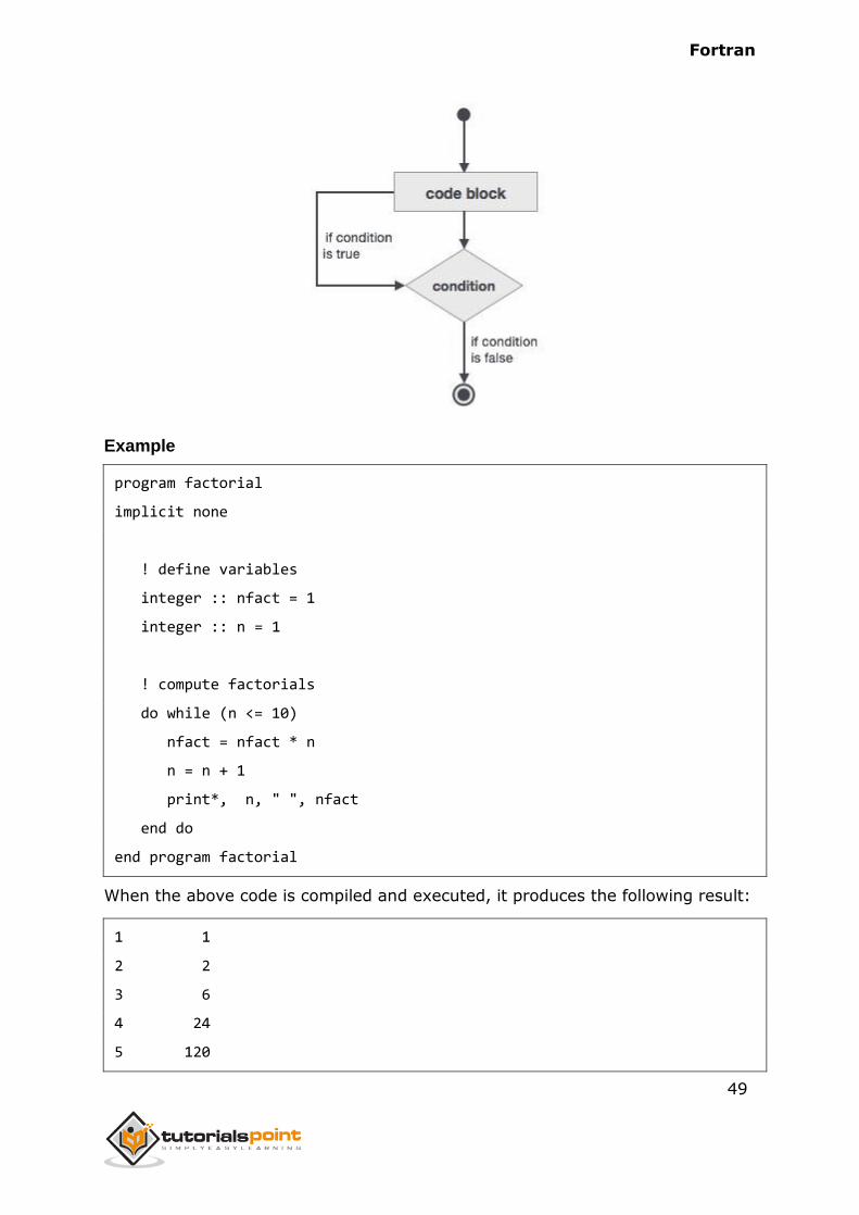
do-while Loop
It repeats a statement or a group of statements while a given condition is true.
It tests the condition before executing the loop body.
Syntax
do while (logical expr)
statements
end do
Flow Diagram
Fortran
49
Example
program factorial
implicit none
! define variables
integer :: nfact = 1
integer :: n = 1
! compute factorials
do while (n <= 10)
nfact = nfact * n
n = n + 1
print*, n, " ", nfact
end do
end program factorial
When the above code is compiled and executed, it produces the following result:
1 1
2 2
3 6
4 24
5 120
Fortran
50
6 720
7 5040
8 40320
9 362880
10 3628800
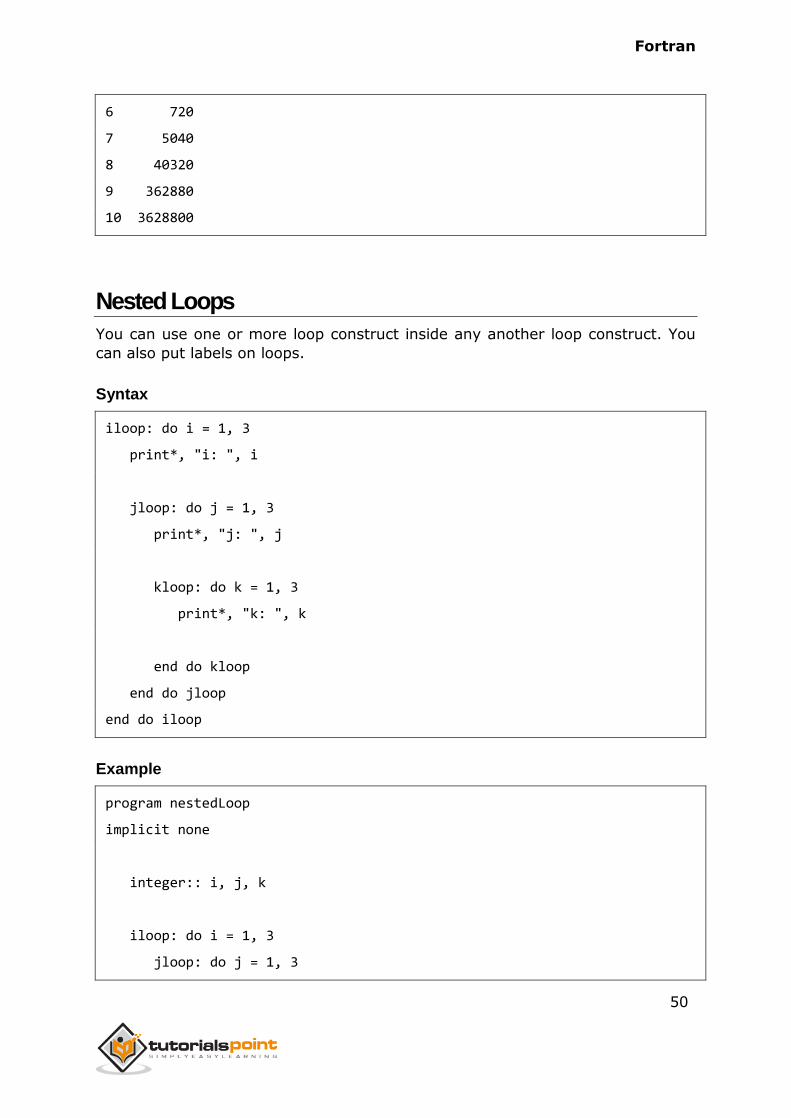
Nested Loops
You can use one or more loop construct inside any another loop construct. You
can also put labels on loops.
Syntax
iloop: do i = 1, 3
print*, "i: ", i
jloop: do j = 1, 3
print*, "j: ", j
kloop: do k = 1, 3
print*, "k: ", k
end do kloop
end do jloop
end do iloop
Example
program nestedLoop
implicit none
integer:: i, j, k
iloop: do i = 1, 3
jloop: do j = 1, 3
Fortran
51
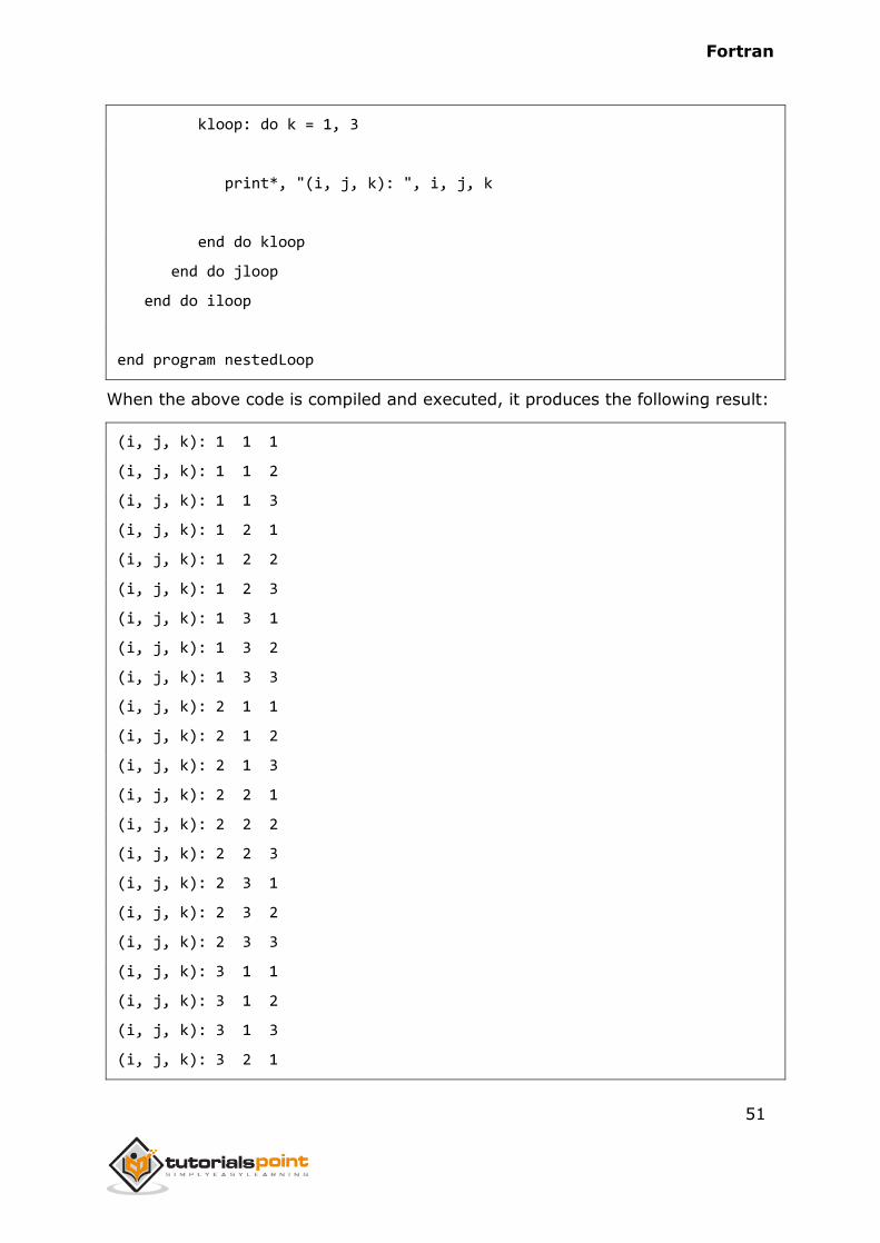
kloop: do k = 1, 3
print*, "(i, j, k): ", i, j, k
end do kloop
end do jloop
end do iloop
end program nestedLoop
When the above code is compiled and executed, it produces the following result:
(i, j, k): 1 1 1
(i, j, k): 1 1 2
(i, j, k): 1 1 3
(i, j, k): 1 2 1
(i, j, k): 1 2 2
(i, j, k): 1 2 3
(i, j, k): 1 3 1
(i, j, k): 1 3 2
(i, j, k): 1 3 3
(i, j, k): 2 1 1
(i, j, k): 2 1 2
(i, j, k): 2 1 3
(i, j, k): 2 2 1
(i, j, k): 2 2 2
(i, j, k): 2 2 3
(i, j, k): 2 3 1
(i, j, k): 2 3 2
(i, j, k): 2 3 3
(i, j, k): 3 1 1
(i, j, k): 3 1 2
(i, j, k): 3 1 3
(i, j, k): 3 2 1
Fortran
52
(i, j, k): 3 2 2
Loop Control Statements
Loop control statements change execution from its normal sequence. When
execution leaves a scope, all automatic objects that were created in that scope
are destroyed.
Fortran supports the following control statements. Click the following links to
check their detail.
Control
Statement
Description
exit If the exit statement is executed, the loop is exited, and
the execution of the program continues at the first
executable statement after the end do statement.
cycle If a cycle statement is executed, the program continues at
the start of the next iteration.
stop If you wish execution of your program to stop, you can
insert a stop statement
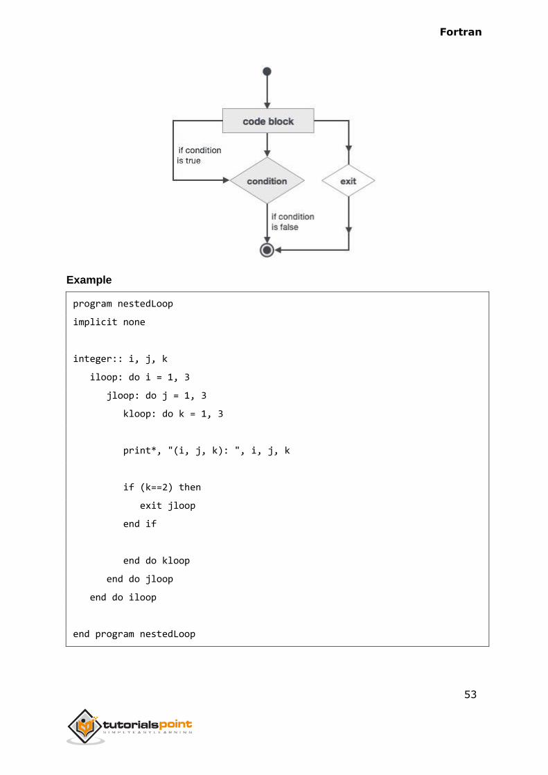
Exit Statement
Exit statement terminates the loop or select case statement, and transfers
execution to the statement immediately following the loop or select.
Flow Diagram
Fortran
53
Example
program nestedLoop
implicit none
integer:: i, j, k
iloop: do i = 1, 3
jloop: do j = 1, 3
kloop: do k = 1, 3
print*, "(i, j, k): ", i, j, k
if (k==2) then
exit jloop
end if
end do kloop
end do jloop
end do iloop
end program nestedLoop
Fortran
54
When the above code is compiled and executed, it produces the following result:
(i, j, k): 1 1 1
(i, j, k): 1 1 2
(i, j, k): 2 1 1
(i, j, k): 2 1 2
(i, j, k): 3 1 1
(i, j, k): 3 1 2
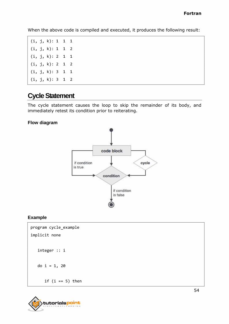
Cycle Statement
The cycle statement causes the loop to skip the remainder of its body, and
immediately retest its condition prior to reiterating.
Flow diagram
Example
program cycle_example
implicit none
integer :: i
do i = 1, 20
if (i == 5) then
Fortran
55
cycle
end if
print*, i
end do
end program cycle_example
When the above code is compiled and executed, it produces the following result:
1
2
3
4
6
7
8
9
10
11
12
13
14
15
16
17
18
19
20
Stop Statement
If you wish execution of your program to cease, you can insert a stop statement.
Example
Fortran
56
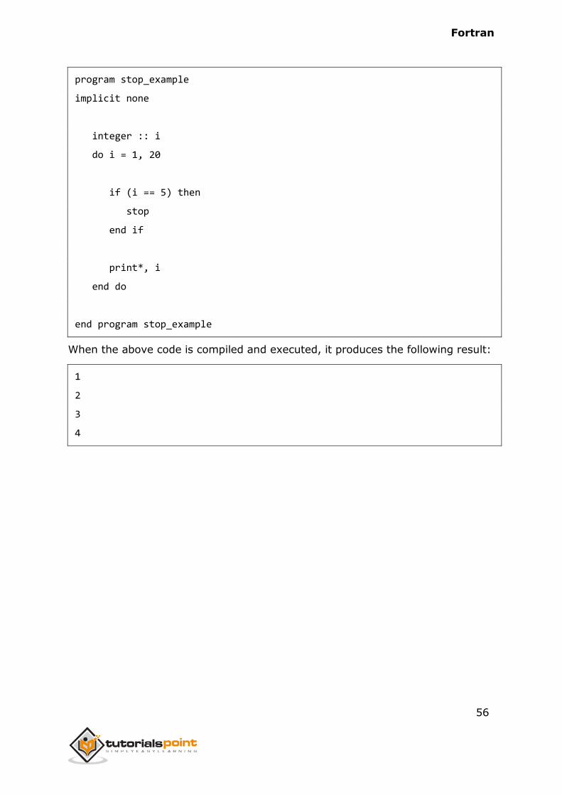
program stop_example
implicit none
integer :: i
do i = 1, 20
if (i == 5) then
stop
end if
print*, i
end do
end program stop_example
When the above code is compiled and executed, it produces the following result:
1
2
3
4
Fortran
57
Numbers in Fortran are represented by three intrinsic data types:
Integer type
Real type
Complex type
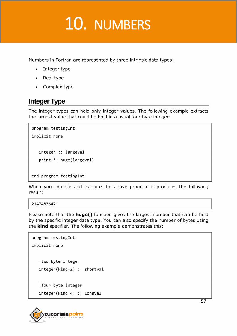
Integer Type
The integer types can hold only integer values. The following example extracts
the largest value that could be hold in a usual four byte integer:
program testingInt
implicit none
integer :: largeval
print *, huge(largeval)
end program testingInt
When you compile and execute the above program it produces the following
result:
2147483647
Please note that the huge() function gives the largest number that can be held
by the specific integer data type. You can also specify the number of bytes using
the kind specifier. The following example demonstrates this:
program testingInt
implicit none
!two byte integer
integer(kind=2) :: shortval
!four byte integer
integer(kind=4) :: longval
10. NUMBERS
Fortran
58
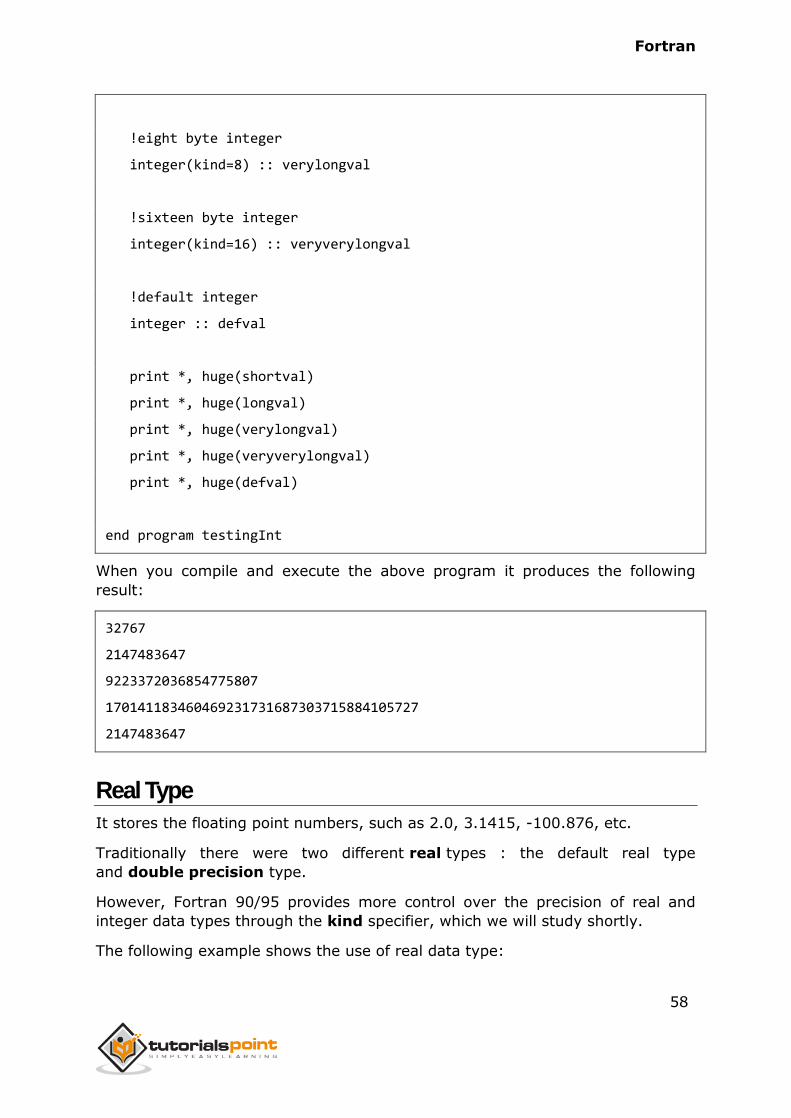
!eight byte integer
integer(kind=8) :: verylongval
!sixteen byte integer
integer(kind=16) :: veryverylongval
!default integer
integer :: defval
print *, huge(shortval)
print *, huge(longval)
print *, huge(verylongval)
print *, huge(veryverylongval)
print *, huge(defval)
end program testingInt
When you compile and execute the above program it produces the following
result:
32767
2147483647
9223372036854775807
170141183460469231731687303715884105727
2147483647
Real Type
It stores the floating point numbers, such as 2.0, 3.1415, -100.876, etc.
Traditionally there were two different real types : the default real type
and double precision type.
However, Fortran 90/95 provides more control over the precision of real and
integer data types through the kind specifier, which we will study shortly.
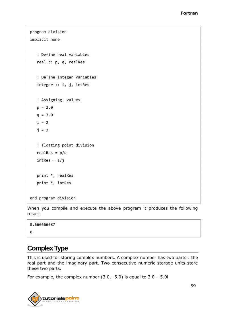
The following example shows the use of real data type:
Fortran
59
program division
implicit none
! Define real variables
real :: p, q, realRes
! Define integer variables
integer :: i, j, intRes
! Assigning values
p = 2.0
q = 3.0
i = 2
j = 3
! floating point division
realRes = p/q
intRes = i/j
print *, realRes
print *, intRes
end program division
When you compile and execute the above program it produces the following
result:
0.666666687
0
Complex Type
This is used for storing complex numbers. A complex number has two parts : the
real part and the imaginary part. Two consecutive numeric storage units store
these two parts.
For example, the complex number (3.0, -5.0) is equal to 3.0 – 5.0i
Fortran
60
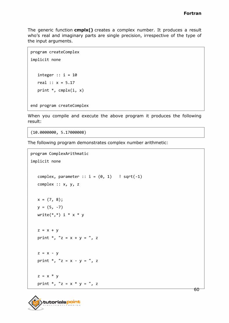
The generic function cmplx() creates a complex number. It produces a result
who’s real and imaginary parts are single precision, irrespective of the type of
the input arguments.
program createComplex
implicit none
integer :: i = 10
real :: x = 5.17
print *, cmplx(i, x)
end program createComplex
When you compile and execute the above program it produces the following
result:
(10.0000000, 5.17000008)
The following program demonstrates complex number arithmetic:
program ComplexArithmatic
implicit none
complex, parameter :: i = (0, 1) ! sqrt(-1)
complex :: x, y, z
x = (7, 8);
y = (5, -7)
write(*,*) i * x * y
z = x + y
print *, "z = x + y = ", z
z = x - y
print *, "z = x - y = ", z
z = x * y
print *, "z = x * y = ", z
Fortran
61
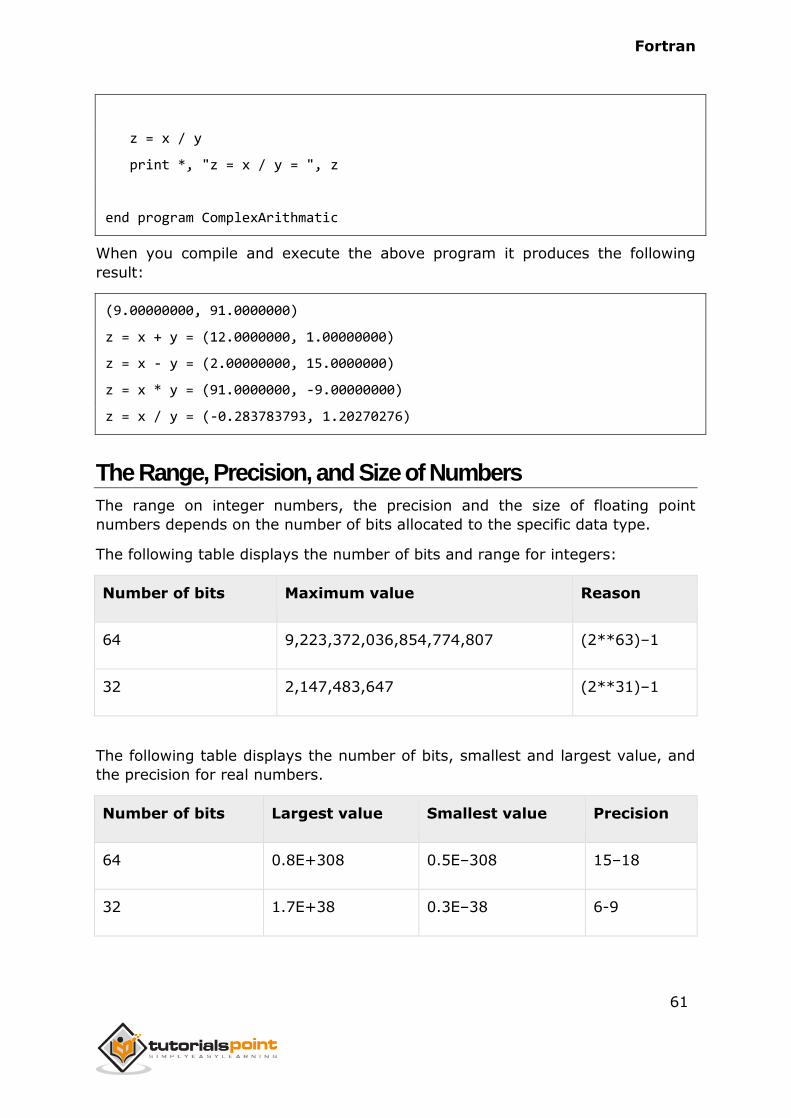
z = x / y
print *, "z = x / y = ", z
end program ComplexArithmatic
When you compile and execute the above program it produces the following
result:
(9.00000000, 91.0000000)
z = x + y = (12.0000000, 1.00000000)
z = x - y = (2.00000000, 15.0000000)
z = x * y = (91.0000000, -9.00000000)
z = x / y = (-0.283783793, 1.20270276)
The Range, Precision, and Size of Numbers
The range on integer numbers, the precision and the size of floating point
numbers depends on the number of bits allocated to the specific data type.
The following table displays the number of bits and range for integers:
Number of bits Maximum value Reason
64 9,223,372,036,854,774,807 (2**63)–1
32 2,147,483,647 (2**31)–1
The following table displays the number of bits, smallest and largest value, and
the precision for real numbers.
Number of bits Largest value Smallest value Precision
64 0.8E+308 0.5E–308 15–18
32 1.7E+38 0.3E–38 6-9
Fortran
62
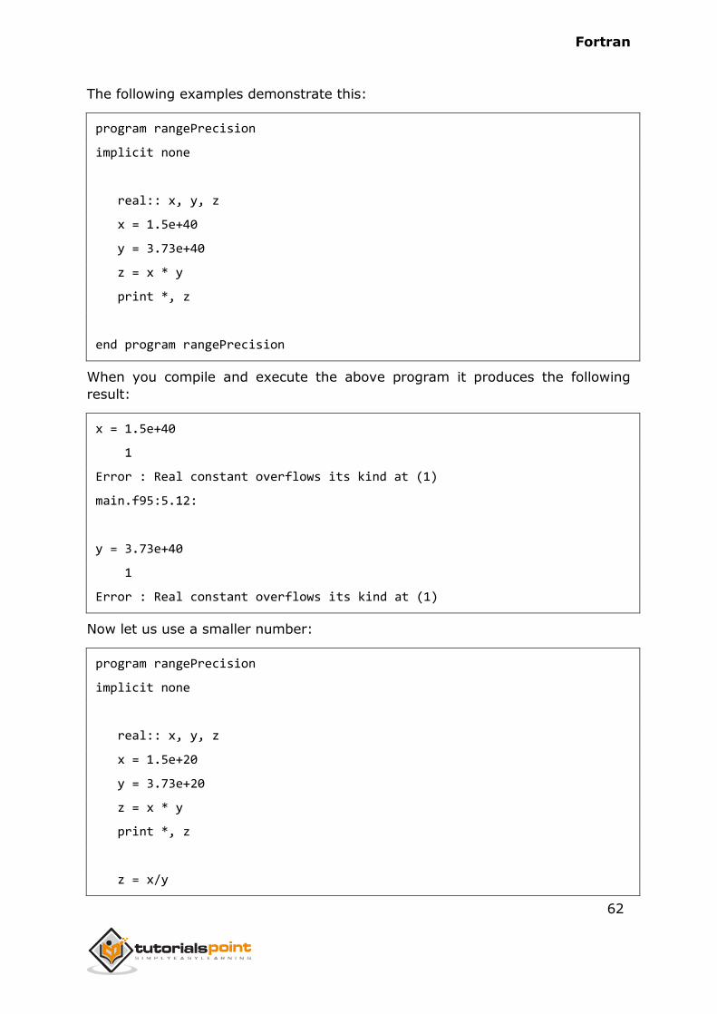
The following examples demonstrate this:
program rangePrecision
implicit none
real:: x, y, z
x = 1.5e+40
y = 3.73e+40
z = x * y
print *, z
end program rangePrecision
When you compile and execute the above program it produces the following
result:
x = 1.5e+40
1
Error : Real constant overflows its kind at (1)
main.f95:5.12:
y = 3.73e+40
1
Error : Real constant overflows its kind at (1)
Now let us use a smaller number:
program rangePrecision
implicit none
real:: x, y, z
x = 1.5e+20
y = 3.73e+20
z = x * y
print *, z
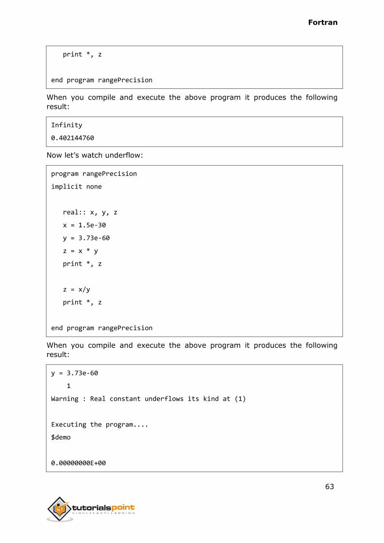
z = x/y
Fortran
63
print *, z
end program rangePrecision
When you compile and execute the above program it produces the following
result:
Infinity
0.402144760
Now let’s watch underflow:
program rangePrecision
implicit none
real:: x, y, z
x = 1.5e-30
y = 3.73e-60
z = x * y
print *, z
z = x/y
print *, z
end program rangePrecision
When you compile and execute the above program it produces the following
result:
y = 3.73e-60
1
Warning : Real constant underflows its kind at (1)
Executing the program....
$demo
0.00000000E+00
Fortran
64
Infinity
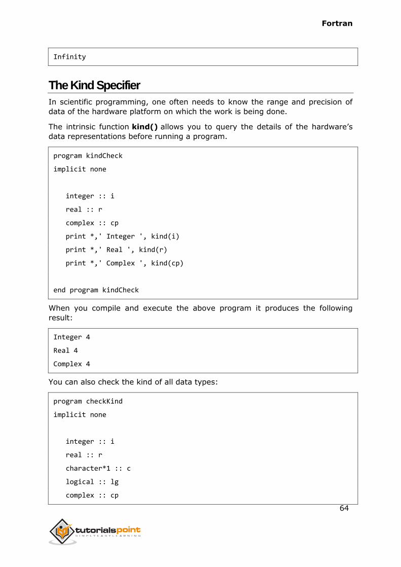
The Kind Specifier
In scientific programming, one often needs to know the range and precision of
data of the hardware platform on which the work is being done.
The intrinsic function kind() allows you to query the details of the hardware’s
data representations before running a program.
program kindCheck
implicit none
integer :: i
real :: r
complex :: cp
print *,' Integer ', kind(i)
print *,' Real ', kind(r)
print *,' Complex ', kind(cp)
end program kindCheck
When you compile and execute the above program it produces the following
result:
Integer 4
Real 4
Complex 4
You can also check the kind of all data types:
program checkKind
implicit none
integer :: i
real :: r
character*1 :: c
logical :: lg
complex :: cp
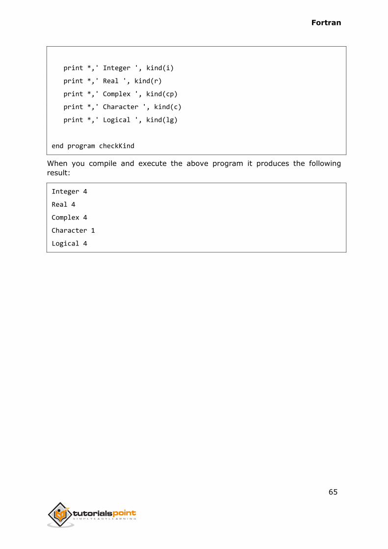
Fortran
65
print *,' Integer ', kind(i)
print *,' Real ', kind(r)
print *,' Complex ', kind(cp)
print *,' Character ', kind(c)
print *,' Logical ', kind(lg)
end program checkKind
When you compile and execute the above program it produces the following
result:
Integer 4
Real 4
Complex 4
Character 1
Logical 4
Fortran
66
The Fortran language can treat characters as single character or contiguous
strings.
Characters could be any symbol taken from the basic character set, i.e., from
the letters, the decimal digits, the underscore, and 21 special characters.
A character constant is a fixed valued character string.
The intrinsic data type character stores characters and strings. The length of
the string can be specified by len specifier. If no length is specified, it is 1. You
can refer individual characters within a string referring by position; the left most
character is at position 1.
Character Declaration
Declaring a character type data is same as other variables:
type-specifier :: variable_name
For example,
character :: reply, sex
you can assign a value like,
reply = ‘N’
sex = ‘F’
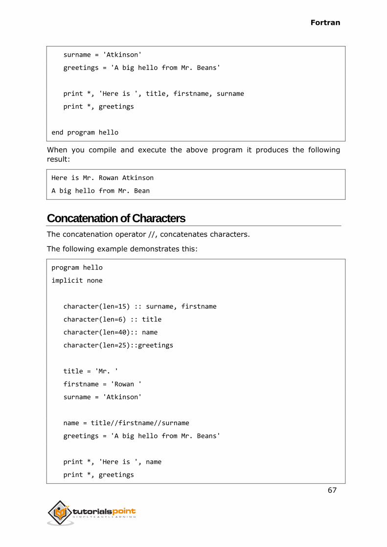
The following example demonstrates declaration and use of character data type:
program hello
implicit none
character(len=15) :: surname, firstname
character(len=6) :: title
character(len=25)::greetings
title = 'Mr. '
firstname = 'Rowan '
11. CHARACTERS
Fortran
67
surname = 'Atkinson'
greetings = 'A big hello from Mr. Beans'
print *, 'Here is ', title, firstname, surname
print *, greetings
end program hello
When you compile and execute the above program it produces the following
result:
Here is Mr. Rowan Atkinson
A big hello from Mr. Bean
Concatenation of Characters
The concatenation operator //, concatenates characters.
The following example demonstrates this:
program hello
implicit none
character(len=15) :: surname, firstname
character(len=6) :: title
character(len=40):: name
character(len=25)::greetings
title = 'Mr. '
firstname = 'Rowan '
surname = 'Atkinson'
name = title//firstname//surname
greetings = 'A big hello from Mr. Beans'
print *, 'Here is ', name
print *, greetings

Fortran
68
end program hello
When you compile and execute the above program it produces the following
result:
Here is Mr.Rowan Atkinson
A big hello from Mr.Bean
Some Character Functions
The following table shows some commonly used character functions along with
the description:
Function Description
len(string) It returns the length of a character string
index(string,sustring) It finds the location of a substring in another string,
returns 0 if not found.
achar(int) It converts an integer into a character
iachar(c) It converts a character into an integer
trim(string) It returns the string with the trailing blanks removed.
scan(string, chars) It searches the "string" from left to right (unless
back=.true.) for the first occurrence of any character
contained in "chars". It returns an integer giving the
position of that character, or zero if none of the
characters in "chars" have been found.
verify(string, chars) It scans the "string" from left to right (unless
back=.true.) for the first occurrence of any character
not contained in "chars". It returns an integer giving
the position of that character, or zero if only the
characters in "chars" have been found
adjustl(string) It left justifies characters contained in the "string"
Fortran
69
adjustr(string) It right justifies characters contained in the "string"
len_trim(string) It returns an integer equal to the length of "string"
(len(string)) minus the number of trailing blanks
repeat(string,ncopy) It returns a string with length equal to "ncopy" times
the length of "string", and containing "ncopy"
concatenated copies of "string"
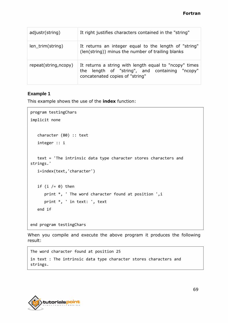
Example 1
This example shows the use of the index function:
program testingChars
implicit none
character (80) :: text
integer :: i
text = 'The intrinsic data type character stores characters and
strings.'
i=index(text,'character')
if (i /= 0) then
print *, ' The word character found at position ',i
print *, ' in text: ', text
end if
end program testingChars
When you compile and execute the above program it produces the following
result:
The word character found at position 25
in text : The intrinsic data type character stores characters and
strings.
Fortran
70
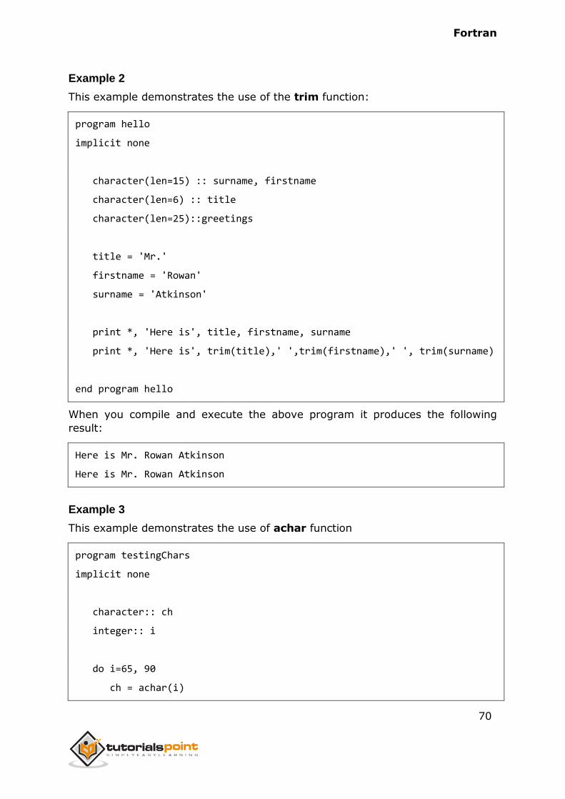
Example 2
This example demonstrates the use of the trim function:
program hello
implicit none
character(len=15) :: surname, firstname
character(len=6) :: title
character(len=25)::greetings
title = 'Mr.'
firstname = 'Rowan'
surname = 'Atkinson'
print *, 'Here is', title, firstname, surname
print *, 'Here is', trim(title),' ',trim(firstname),' ', trim(surname)
end program hello
When you compile and execute the above program it produces the following
result:
Here is Mr. Rowan Atkinson
Here is Mr. Rowan Atkinson
Example 3
This example demonstrates the use of achar function
program testingChars
implicit none
character:: ch
integer:: i
do i=65, 90
ch = achar(i)
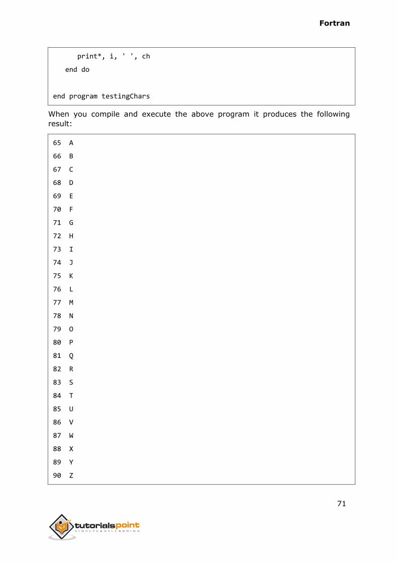
Fortran
71
print*, i, ' ', ch
end do
end program testingChars
When you compile and execute the above program it produces the following
result:
65 A
66 B
67 C
68 D
69 E
70 F
71 G
72 H
73 I
74 J
75 K
76 L
77 M
78 N
79 O
80 P
81 Q
82 R
83 S
84 T
85 U
86 V
87 W
88 X
89 Y
90 Z
Fortran
72
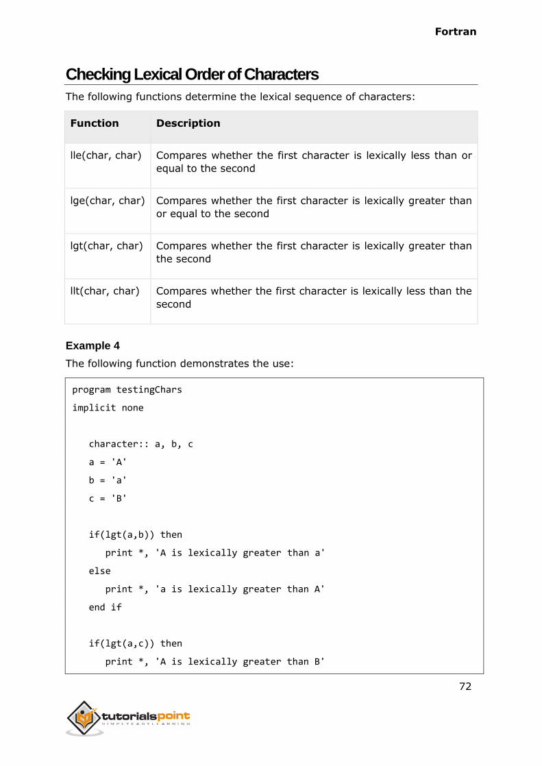
Checking Lexical Order of Characters
The following functions determine the lexical sequence of characters:
Function Description
lle(char, char) Compares whether the first character is lexically less than or
equal to the second
lge(char, char) Compares whether the first character is lexically greater than
or equal to the second
lgt(char, char) Compares whether the first character is lexically greater than
the second
llt(char, char) Compares whether the first character is lexically less than the
second
Example 4
The following function demonstrates the use:
program testingChars
implicit none
character:: a, b, c
a = 'A'
b = 'a'
c = 'B'
if(lgt(a,b)) then
print *, 'A is lexically greater than a'
else
print *, 'a is lexically greater than A'
end if
if(lgt(a,c)) then
print *, 'A is lexically greater than B'
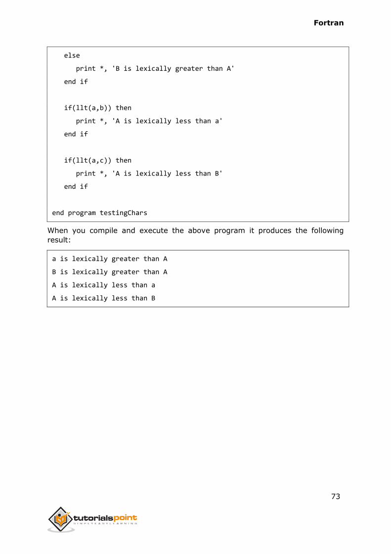
Fortran
73
else
print *, 'B is lexically greater than A'
end if
if(llt(a,b)) then
print *, 'A is lexically less than a'
end if
if(llt(a,c)) then
print *, 'A is lexically less than B'
end if
end program testingChars
When you compile and execute the above program it produces the following
result:
a is lexically greater than A
B is lexically greater than A
A is lexically less than a
A is lexically less than B
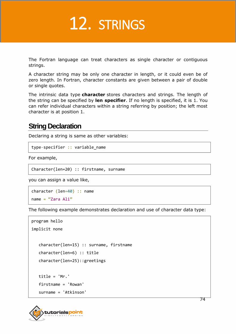
Fortran
74
The Fortran language can treat characters as single character or contiguous
strings.
A character string may be only one character in length, or it could even be of
zero length. In Fortran, character constants are given between a pair of double
or single quotes.
The intrinsic data type character stores characters and strings. The length of
the string can be specified by len specifier. If no length is specified, it is 1. You
can refer individual characters within a string referring by position; the left most
character is at position 1.
String Declaration
Declaring a string is same as other variables:
type-specifier :: variable_name
For example,
Character(len=20) :: firstname, surname
you can assign a value like,
character (len=40) :: name
name = “Zara Ali”
The following example demonstrates declaration and use of character data type:
program hello
implicit none
character(len=15) :: surname, firstname
character(len=6) :: title
character(len=25)::greetings
title = 'Mr.'
firstname = 'Rowan'
surname = 'Atkinson'
12. STRINGS
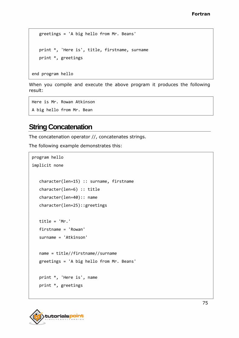
Fortran
75
greetings = 'A big hello from Mr. Beans'
print *, 'Here is', title, firstname, surname
print *, greetings
end program hello
When you compile and execute the above program it produces the following
result:
Here is Mr. Rowan Atkinson
A big hello from Mr. Bean
String Concatenation
The concatenation operator //, concatenates strings.
The following example demonstrates this:
program hello
implicit none
character(len=15) :: surname, firstname
character(len=6) :: title
character(len=40):: name
character(len=25)::greetings
title = 'Mr.'
firstname = 'Rowan'
surname = 'Atkinson'
name = title//firstname//surname
greetings = 'A big hello from Mr. Beans'
print *, 'Here is', name
print *, greetings
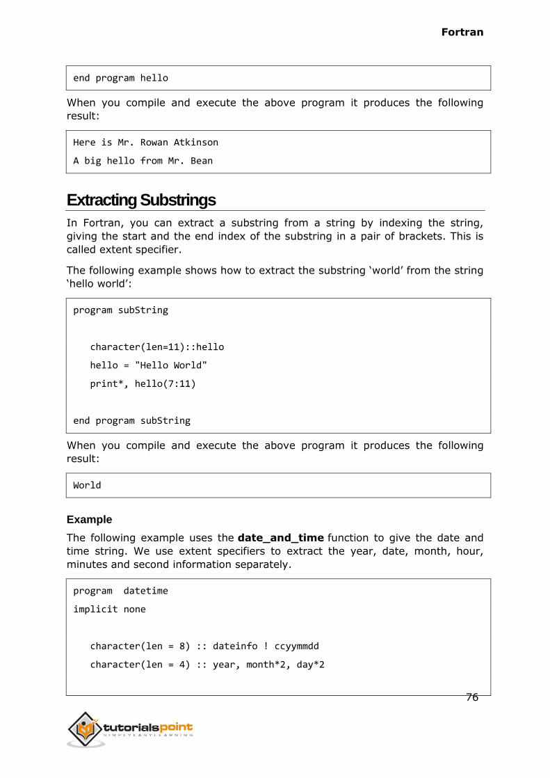
Fortran
76
end program hello
When you compile and execute the above program it produces the following
result:
Here is Mr. Rowan Atkinson
A big hello from Mr. Bean
Extracting Substrings
In Fortran, you can extract a substring from a string by indexing the string,
giving the start and the end index of the substring in a pair of brackets. This is
called extent specifier.
The following example shows how to extract the substring ‘world’ from the string
‘hello world’:
program subString
character(len=11)::hello
hello = "Hello World"
print*, hello(7:11)
end program subString
When you compile and execute the above program it produces the following
result:
World
Example
The following example uses the date_and_time function to give the date and
time string. We use extent specifiers to extract the year, date, month, hour,
minutes and second information separately.
program datetime
implicit none
character(len = 8) :: dateinfo ! ccyymmdd
character(len = 4) :: year, month*2, day*2

Fortran
77
character(len = 10) :: timeinfo ! hhmmss.sss
character(len = 2) :: hour, minute, second*6
call date_and_time(dateinfo, timeinfo)
! let’s break dateinfo into year, month and day.
! dateinfo has a form of ccyymmdd, where cc = century, yy = year
! mm = month and dd = day
year = dateinfo(1:4)
month = dateinfo(5:6)
day = dateinfo(7:8)
print*, 'Date String:', dateinfo
print*, 'Year:', year
print *,'Month:', month
print *,'Day:', day
! let’s break timeinfo into hour, minute and second.
! timeinfo has a form of hhmmss.sss, where h = hour, m = minute
! and s = second
hour = timeinfo(1:2)
minute = timeinfo(3:4)
second = timeinfo(5:10)
print*, 'Time String:', timeinfo
print*, 'Hour:', hour
print*, 'Minute:', minute
print*, 'Second:', second
end program datetime
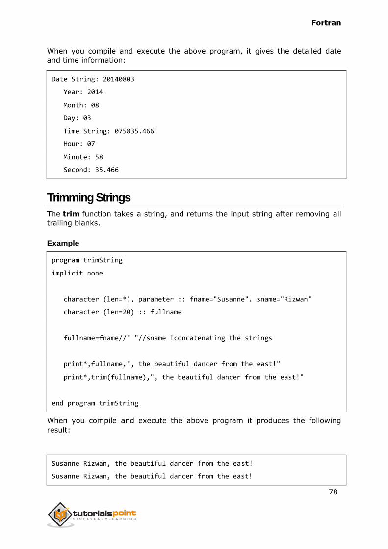
Fortran
78
When you compile and execute the above program, it gives the detailed date
and time information:
Date String: 20140803
Year: 2014
Month: 08
Day: 03
Time String: 075835.466
Hour: 07
Minute: 58
Second: 35.466
Trimming Strings
The trim function takes a string, and returns the input string after removing all
trailing blanks.
Example
program trimString
implicit none
character (len=*), parameter :: fname="Susanne", sname="Rizwan"
character (len=20) :: fullname
fullname=fname//" "//sname !concatenating the strings
print*,fullname,", the beautiful dancer from the east!"
print*,trim(fullname),", the beautiful dancer from the east!"
end program trimString
When you compile and execute the above program it produces the following
result:
Susanne Rizwan, the beautiful dancer from the east!
Susanne Rizwan, the beautiful dancer from the east!
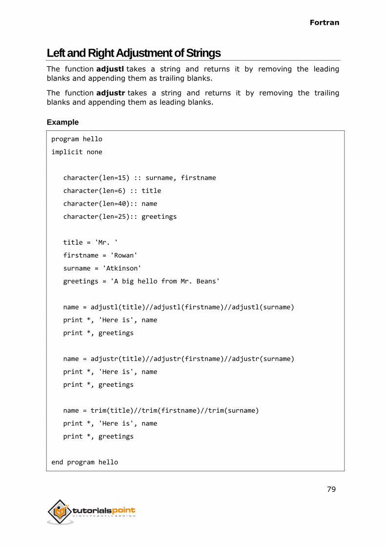
Fortran
79
Left and Right Adjustment of Strings
The function adjustl takes a string and returns it by removing the leading
blanks and appending them as trailing blanks.
The function adjustr takes a string and returns it by removing the trailing
blanks and appending them as leading blanks.
Example
program hello
implicit none
character(len=15) :: surname, firstname
character(len=6) :: title
character(len=40):: name
character(len=25):: greetings
title = 'Mr. '
firstname = 'Rowan'
surname = 'Atkinson'
greetings = 'A big hello from Mr. Beans'
name = adjustl(title)//adjustl(firstname)//adjustl(surname)
print *, 'Here is', name
print *, greetings
name = adjustr(title)//adjustr(firstname)//adjustr(surname)
print *, 'Here is', name
print *, greetings
name = trim(title)//trim(firstname)//trim(surname)
print *, 'Here is', name
print *, greetings
end program hello
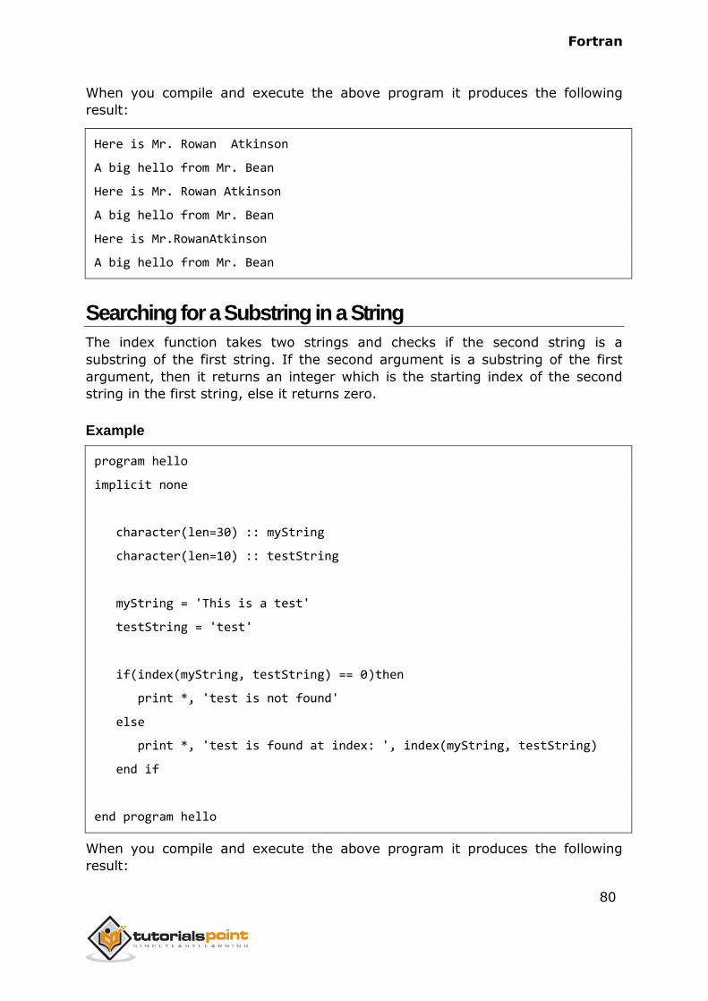
Fortran
80
When you compile and execute the above program it produces the following
result:
Here is Mr. Rowan Atkinson
A big hello from Mr. Bean
Here is Mr. Rowan Atkinson
A big hello from Mr. Bean
Here is Mr.RowanAtkinson
A big hello from Mr. Bean
Searching for a Substring in a String
The index function takes two strings and checks if the second string is a
substring of the first string. If the second argument is a substring of the first
argument, then it returns an integer which is the starting index of the second
string in the first string, else it returns zero.
Example
program hello
implicit none
character(len=30) :: myString
character(len=10) :: testString
myString = 'This is a test'
testString = 'test'
if(index(myString, testString) == 0)then
print *, 'test is not found'
else
print *, 'test is found at index: ', index(myString, testString)
end if
end program hello
When you compile and execute the above program it produces the following
result:

Fortran
81
test is found at index: 11
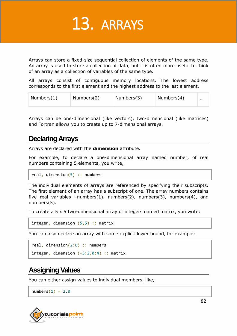
Fortran
82
Arrays can store a fixed-size sequential collection of elements of the same type.
An array is used to store a collection of data, but it is often more useful to think
of an array as a collection of variables of the same type.
All arrays consist of contiguous memory locations. The lowest address
corresponds to the first element and the highest address to the last element.
Numbers(1) Numbers(2) Numbers(3) Numbers(4) …
Arrays can be one-dimensional (like vectors), two-dimensional (like matrices)
and Fortran allows you to create up to 7-dimensional arrays.
Declaring Arrays
Arrays are declared with the dimension attribute.
For example, to declare a one-dimensional array named number, of real
numbers containing 5 elements, you write,
real, dimension(5) :: numbers
The individual elements of arrays are referenced by specifying their subscripts.
The first element of an array has a subscript of one. The array numbers contains
five real variables –numbers(1), numbers(2), numbers(3), numbers(4), and
numbers(5).
To create a 5 x 5 two-dimensional array of integers named matrix, you write:
integer, dimension (5,5) :: matrix
You can also declare an array with some explicit lower bound, for example:
real, dimension(2:6) :: numbers
integer, dimension (-3:2,0:4) :: matrix
Assigning Values
You can either assign values to individual members, like,
numbers(1) = 2.0
13. ARRAYS
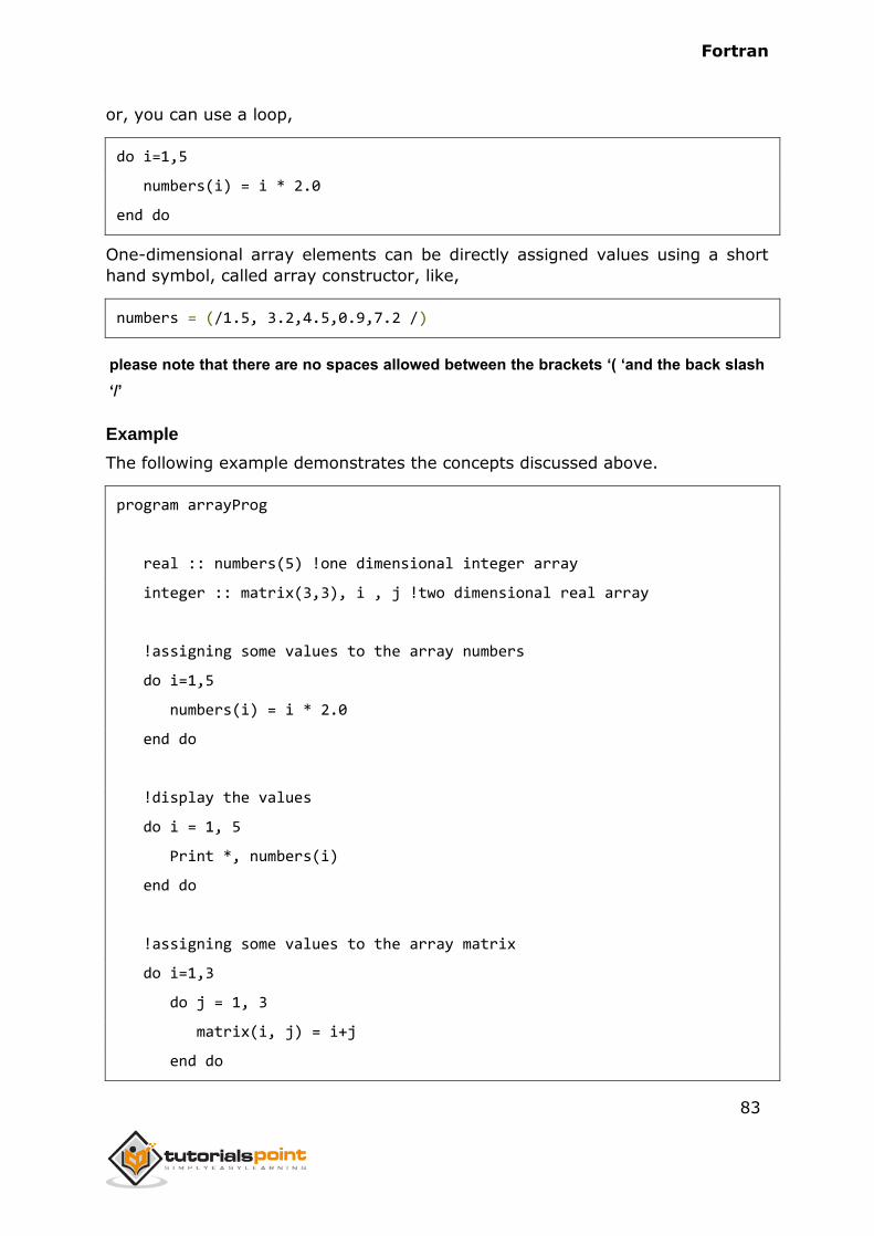
Fortran
83
or, you can use a loop,
do i=1,5
numbers(i) = i * 2.0
end do
One-dimensional array elements can be directly assigned values using a short
hand symbol, called array constructor, like,
numbers = (/1.5, 3.2,4.5,0.9,7.2 /)
please note that there are no spaces allowed between the brackets ‘( ‘and the back slash
‘/’
Example
The following example demonstrates the concepts discussed above.
program arrayProg
real :: numbers(5) !one dimensional integer array
integer :: matrix(3,3), i , j !two dimensional real array
!assigning some values to the array numbers
do i=1,5
numbers(i) = i * 2.0
end do
!display the values
do i = 1, 5
Print *, numbers(i)
end do
!assigning some values to the array matrix
do i=1,3
do j = 1, 3
matrix(i, j) = i+j
end do
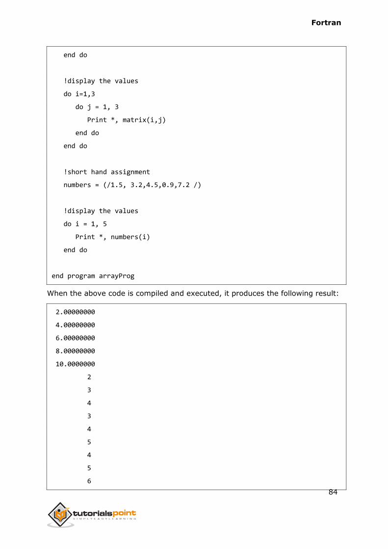
Fortran
84
end do
!display the values
do i=1,3
do j = 1, 3
Print *, matrix(i,j)
end do
end do
!short hand assignment
numbers = (/1.5, 3.2,4.5,0.9,7.2 /)
!display the values
do i = 1, 5
Print *, numbers(i)
end do
end program arrayProg
When the above code is compiled and executed, it produces the following result:
2.00000000
4.00000000
6.00000000
8.00000000
10.0000000
2
3
4
3
4
5
4
5
6
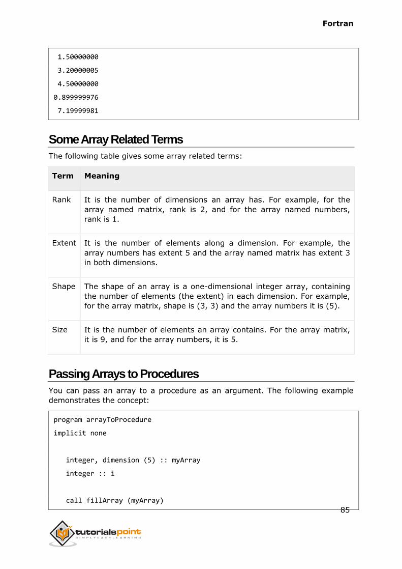
Fortran
85
1.50000000
3.20000005
4.50000000
0.899999976
7.19999981
Some Array Related Terms
The following table gives some array related terms:
Term Meaning
Rank It is the number of dimensions an array has. For example, for the
array named matrix, rank is 2, and for the array named numbers,
rank is 1.
Extent It is the number of elements along a dimension. For example, the
array numbers has extent 5 and the array named matrix has extent 3
in both dimensions.
Shape The shape of an array is a one-dimensional integer array, containing
the number of elements (the extent) in each dimension. For example,
for the array matrix, shape is (3, 3) and the array numbers it is (5).
Size It is the number of elements an array contains. For the array matrix,
it is 9, and for the array numbers, it is 5.
Passing Arrays to Procedures
You can pass an array to a procedure as an argument. The following example
demonstrates the concept:
program arrayToProcedure
implicit none
integer, dimension (5) :: myArray
integer :: i
call fillArray (myArray)
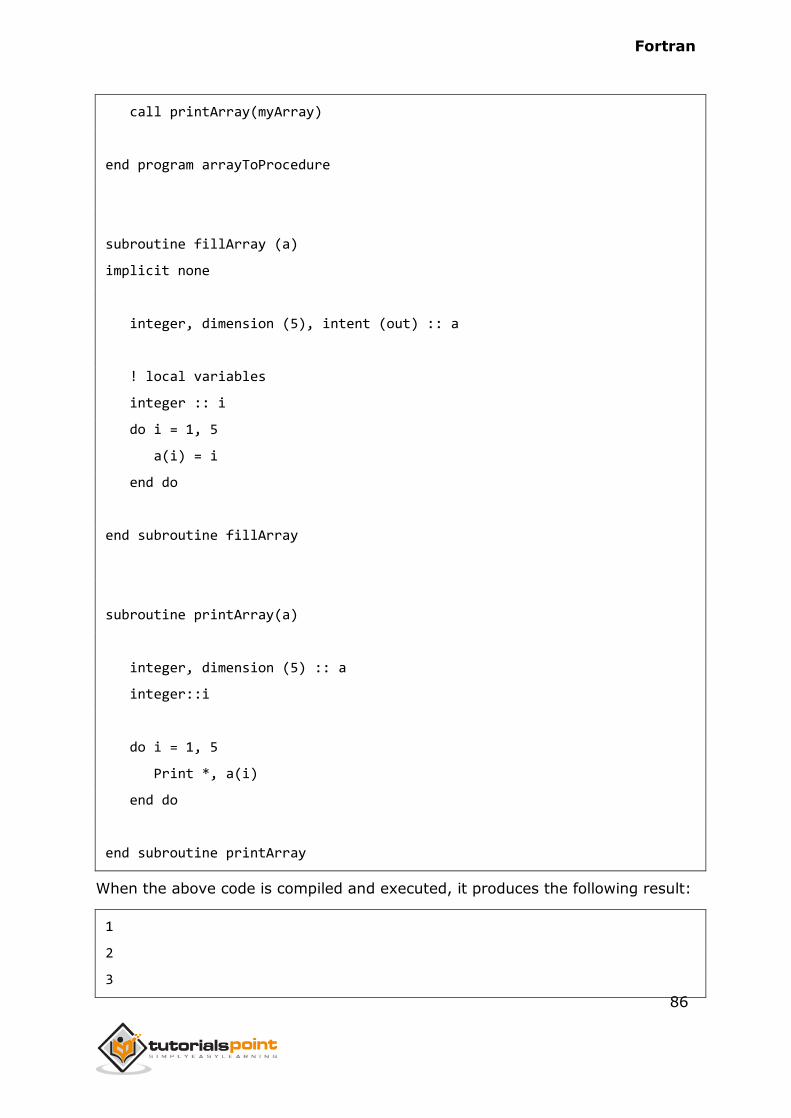
Fortran
86
call printArray(myArray)
end program arrayToProcedure
subroutine fillArray (a)
implicit none
integer, dimension (5), intent (out) :: a
! local variables
integer :: i
do i = 1, 5
a(i) = i
end do
end subroutine fillArray
subroutine printArray(a)
integer, dimension (5) :: a
integer::i
do i = 1, 5
Print *, a(i)
end do
end subroutine printArray
When the above code is compiled and executed, it produces the following result:
1
2
3
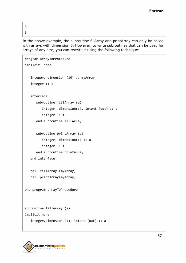
Fortran
87
4
5
In the above example, the subroutine fillArray and printArray can only be called
with arrays with dimension 5. However, to write subroutines that can be used for
arrays of any size, you can rewrite it using the following technique:
program arrayToProcedure
implicit none
integer, dimension (10) :: myArray
integer :: i
interface
subroutine fillArray (a)
integer, dimension(:), intent (out) :: a
integer :: i
end subroutine fillArray
subroutine printArray (a)
integer, dimension(:) :: a
integer :: i
end subroutine printArray
end interface
call fillArray (myArray)
call printArray(myArray)
end program arrayToProcedure
subroutine fillArray (a)
implicit none
integer,dimension (:), intent (out) :: a
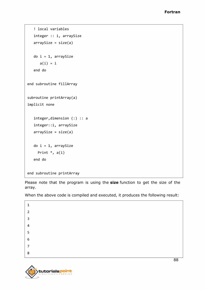
Fortran
88
! local variables
integer :: i, arraySize
arraySize = size(a)
do i = 1, arraySize
a(i) = i
end do
end subroutine fillArray
subroutine printArray(a)
implicit none
integer,dimension (:) :: a
integer::i, arraySize
arraySize = size(a)
do i = 1, arraySize
Print *, a(i)
end do
end subroutine printArray
Please note that the program is using the size function to get the size of the
array.
When the above code is compiled and executed, it produces the following result:
1
2
3
4
5
6
7
8
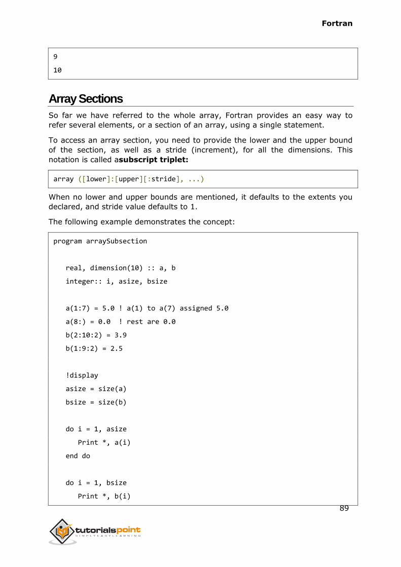
Fortran
89
9
10
Array Sections
So far we have referred to the whole array, Fortran provides an easy way to
refer several elements, or a section of an array, using a single statement.
To access an array section, you need to provide the lower and the upper bound
of the section, as well as a stride (increment), for all the dimensions. This
notation is called asubscript triplet:
array ([lower]:[upper][:stride], ...)
When no lower and upper bounds are mentioned, it defaults to the extents you
declared, and stride value defaults to 1.
The following example demonstrates the concept:
program arraySubsection
real, dimension(10) :: a, b
integer:: i, asize, bsize
a(1:7) = 5.0 ! a(1) to a(7) assigned 5.0
a(8:) = 0.0 ! rest are 0.0
b(2:10:2) = 3.9
b(1:9:2) = 2.5
!display
asize = size(a)
bsize = size(b)
do i = 1, asize
Print *, a(i)
end do
do i = 1, bsize
Print *, b(i)
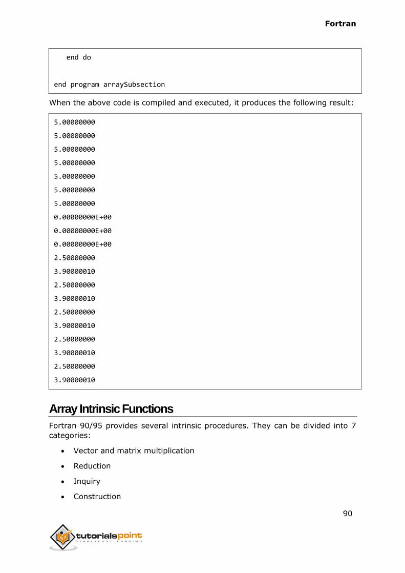
Fortran
90
end do
end program arraySubsection
When the above code is compiled and executed, it produces the following result:
5.00000000
5.00000000
5.00000000
5.00000000
5.00000000
5.00000000
5.00000000
0.00000000E+00
0.00000000E+00
0.00000000E+00
2.50000000
3.90000010
2.50000000
3.90000010
2.50000000
3.90000010
2.50000000
3.90000010
2.50000000
3.90000010
Array Intrinsic Functions
Fortran 90/95 provides several intrinsic procedures. They can be divided into 7
categories:
Vector and matrix multiplication
Reduction
Inquiry
Construction
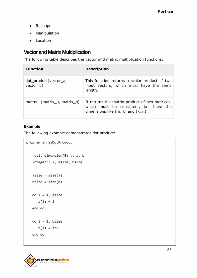
Fortran
91
Reshape
Manipulation
Location
Vector and Matrix Multiplication
The following table describes the vector and matrix multiplication functions:
Function Description
dot_product(vector_a,
vector_b)
This function returns a scalar product of two
input vectors, which must have the same
length.
matmul (matrix_a, matrix_b) It returns the matrix product of two matrices,
which must be consistent, i.e. have the
dimensions like (m, k) and (k, n)
Example
The following example demonstrates dot product:
program arrayDotProduct
real, dimension(5) :: a, b
integer:: i, asize, bsize
asize = size(a)
bsize = size(b)
do i = 1, asize
a(i) = i
end do
do i = 1, bsize
b(i) = i*2
end do
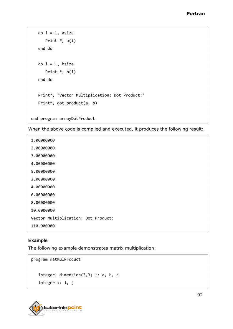
Fortran
92
do i = 1, asize
Print *, a(i)
end do
do i = 1, bsize
Print *, b(i)
end do
Print*, 'Vector Multiplication: Dot Product:'
Print*, dot_product(a, b)
end program arrayDotProduct
When the above code is compiled and executed, it produces the following result:
1.00000000
2.00000000
3.00000000
4.00000000
5.00000000
2.00000000
4.00000000
6.00000000
8.00000000
10.0000000
Vector Multiplication: Dot Product:
110.000000
Example
The following example demonstrates matrix multiplication:
program matMulProduct
integer, dimension(3,3) :: a, b, c
integer :: i, j
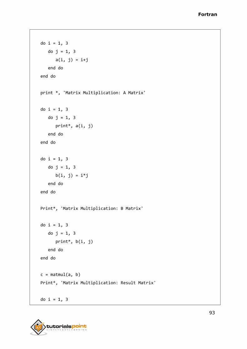
Fortran
93
do i = 1, 3
do j = 1, 3
a(i, j) = i+j
end do
end do
print *, 'Matrix Multiplication: A Matrix'
do i = 1, 3
do j = 1, 3
print*, a(i, j)
end do
end do
do i = 1, 3
do j = 1, 3
b(i, j) = i*j
end do
end do
Print*, 'Matrix Multiplication: B Matrix'
do i = 1, 3
do j = 1, 3
print*, b(i, j)
end do
end do
c = matmul(a, b)
Print*, 'Matrix Multiplication: Result Matrix'
do i = 1, 3
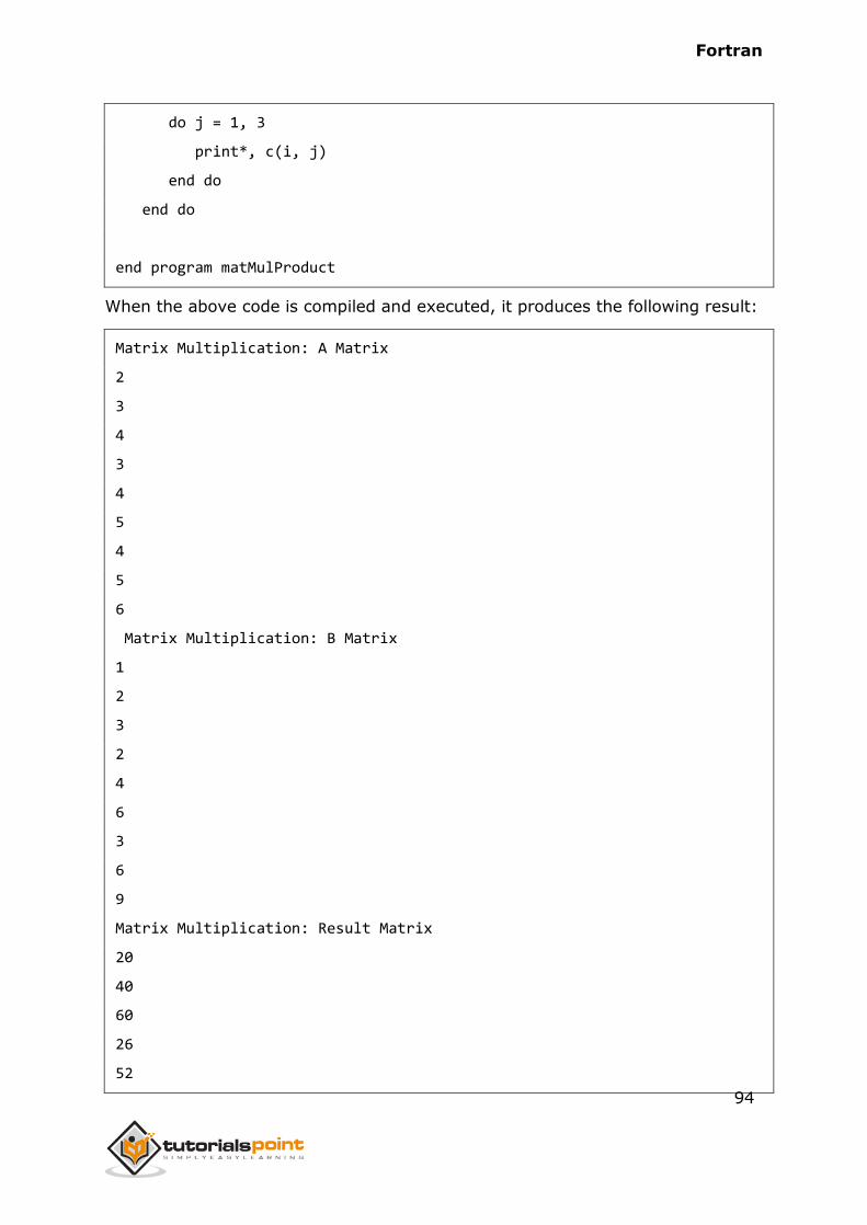
Fortran
94
do j = 1, 3
print*, c(i, j)
end do
end do
end program matMulProduct
When the above code is compiled and executed, it produces the following result:
Matrix Multiplication: A Matrix
2
3
4
3
4
5
4
5
6
Matrix Multiplication: B Matrix
1
2
3
2
4
6
3
6
9
Matrix Multiplication: Result Matrix
20
40
60
26
52
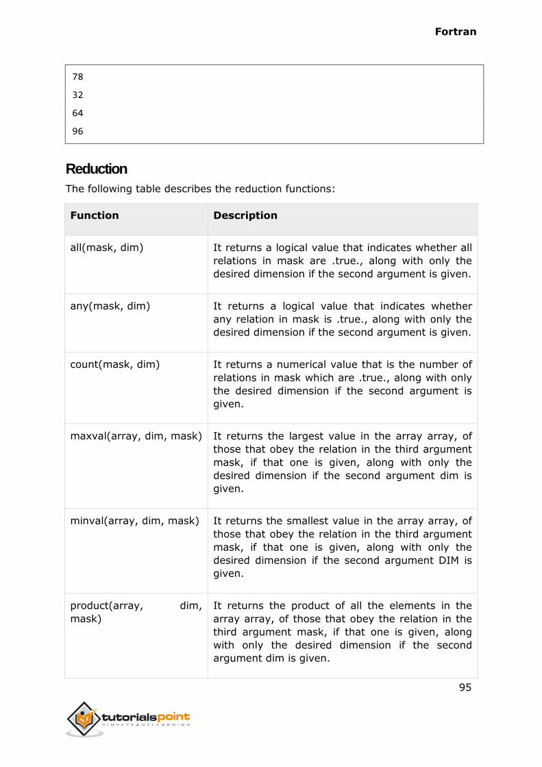
Fortran
95
78
32
64
96
Reduction
The following table describes the reduction functions:
Function Description
all(mask, dim) It returns a logical value that indicates whether all
relations in mask are .true., along with only the
desired dimension if the second argument is given.
any(mask, dim) It returns a logical value that indicates whether
any relation in mask is .true., along with only the
desired dimension if the second argument is given.
count(mask, dim) It returns a numerical value that is the number of
relations in mask which are .true., along with only
the desired dimension if the second argument is
given.
maxval(array, dim, mask) It returns the largest value in the array array, of
those that obey the relation in the third argument
mask, if that one is given, along with only the
desired dimension if the second argument dim is
given.
minval(array, dim, mask) It returns the smallest value in the array array, of
those that obey the relation in the third argument
mask, if that one is given, along with only the
desired dimension if the second argument DIM is
given.
product(array, dim,
mask)
It returns the product of all the elements in the
array array, of those that obey the relation in the
third argument mask, if that one is given, along
with only the desired dimension if the second
argument dim is given.
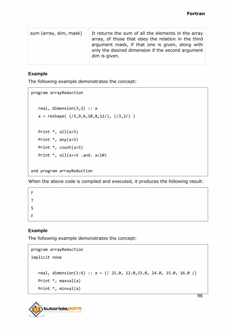
Fortran
96
sum (array, dim, mask) It returns the sum of all the elements in the array
array, of those that obey the relation in the third
argument mask, if that one is given, along with
only the desired dimension if the second argument
dim is given.
Example
The following example demonstrates the concept:
program arrayReduction
real, dimension(3,2) :: a
a = reshape( (/5,9,6,10,8,12/), (/3,2/) )
Print *, all(a>5)
Print *, any(a>5)
Print *, count(a>5)
Print *, all(a>=5 .and. a<10)
end program arrayReduction
When the above code is compiled and executed, it produces the following result:
F
T
5
F
Example
The following example demonstrates the concept:
program arrayReduction
implicit none
real, dimension(1:6) :: a = (/ 21.0, 12.0,33.0, 24.0, 15.0, 16.0 /)
Print *, maxval(a)
Print *, minval(a)
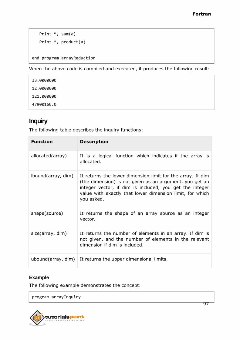
Fortran
97
Print *, sum(a)
Print *, product(a)
end program arrayReduction
When the above code is compiled and executed, it produces the following result:
33.0000000
12.0000000
121.000000
47900160.0
Inquiry
The following table describes the inquiry functions:
Function Description
allocated(array) It is a logical function which indicates if the array is
allocated.
lbound(array, dim) It returns the lower dimension limit for the array. If dim
(the dimension) is not given as an argument, you get an
integer vector, if dim is included, you get the integer
value with exactly that lower dimension limit, for which
you asked.
shape(source) It returns the shape of an array source as an integer
vector.
size(array, dim) It returns the number of elements in an array. If dim is
not given, and the number of elements in the relevant
dimension if dim is included.
ubound(array, dim) It returns the upper dimensional limits.
Example
The following example demonstrates the concept:
program arrayInquiry
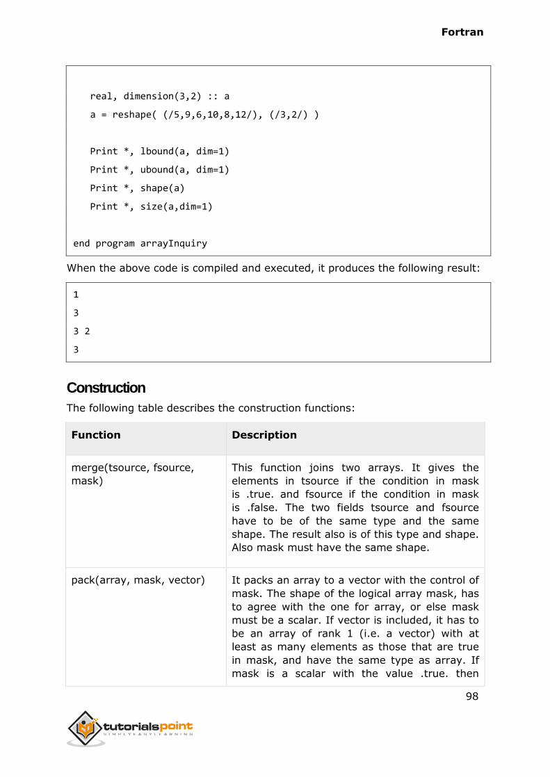
Fortran
98
real, dimension(3,2) :: a
a = reshape( (/5,9,6,10,8,12/), (/3,2/) )
Print *, lbound(a, dim=1)
Print *, ubound(a, dim=1)
Print *, shape(a)
Print *, size(a,dim=1)
end program arrayInquiry
When the above code is compiled and executed, it produces the following result:
1
3
3 2
3
Construction
The following table describes the construction functions:
Function Description
merge(tsource, fsource,
mask)
This function joins two arrays. It gives the
elements in tsource if the condition in mask
is .true. and fsource if the condition in mask
is .false. The two fields tsource and fsource
have to be of the same type and the same
shape. The result also is of this type and shape.
Also mask must have the same shape.
pack(array, mask, vector) It packs an array to a vector with the control of
mask. The shape of the logical array mask, has
to agree with the one for array, or else mask
must be a scalar. If vector is included, it has to
be an array of rank 1 (i.e. a vector) with at
least as many elements as those that are true
in mask, and have the same type as array. If
mask is a scalar with the value .true. then
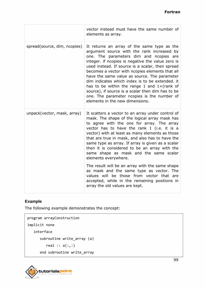
Fortran
99
vector instead must have the same number of
elements as array.
spread(source, dim, ncopies) It returns an array of the same type as the
argument source with the rank increased by
one. The parameters dim and ncopies are
integer. if ncopies is negative the value zero is
used instead. If source is a scalar, then spread
becomes a vector with ncopies elements that all
have the same value as source. The parameter
dim indicates which index is to be extended. it
has to be within the range 1 and 1+(rank of
source), if source is a scalar then dim has to be
one. The parameter ncopies is the number of
elements in the new dimensions.
unpack(vector, mask, array) It scatters a vector to an array under control of
mask. The shape of the logical array mask has
to agree with the one for array. The array
vector has to have the rank 1 (i.e. it is a
vector) with at least as many elements as those
that are true in mask, and also has to have the
same type as array. If array is given as a scalar
then it is considered to be an array with the
same shape as mask and the same scalar
elements everywhere.
The result will be an array with the same shape
as mask and the same type as vector. The
values will be those from vector that are
accepted, while in the remaining positions in
array the old values are kept.
Example
The following example demonstrates the concept:
program arrayConstruction
implicit none
interface
subroutine write_array (a)
real :: a(:,:)
end subroutine write_array
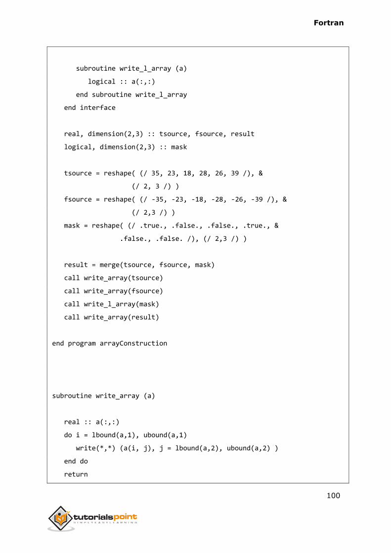
Fortran
100
subroutine write_l_array (a)
logical :: a(:,:)
end subroutine write_l_array
end interface
real, dimension(2,3) :: tsource, fsource, result
logical, dimension(2,3) :: mask
tsource = reshape( (/ 35, 23, 18, 28, 26, 39 /), &
(/ 2, 3 /) )
fsource = reshape( (/ -35, -23, -18, -28, -26, -39 /), &
(/ 2,3 /) )
mask = reshape( (/ .true., .false., .false., .true., &
.false., .false. /), (/ 2,3 /) )
result = merge(tsource, fsource, mask)
call write_array(tsource)
call write_array(fsource)
call write_l_array(mask)
call write_array(result)
end program arrayConstruction
subroutine write_array (a)
real :: a(:,:)
do i = lbound(a,1), ubound(a,1)
write(*,*) (a(i, j), j = lbound(a,2), ubound(a,2) )
end do
return
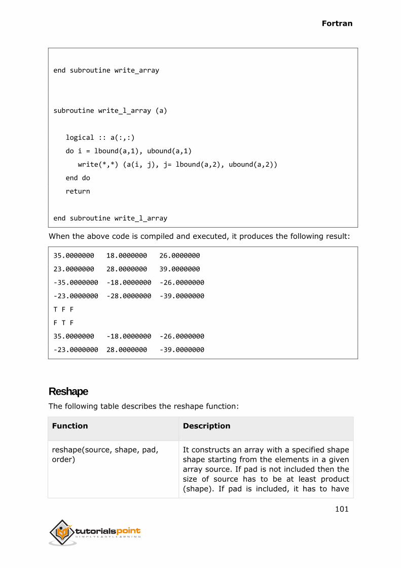
Fortran
101
end subroutine write_array
subroutine write_l_array (a)
logical :: a(:,:)
do i = lbound(a,1), ubound(a,1)
write(*,*) (a(i, j), j= lbound(a,2), ubound(a,2))
end do
return
end subroutine write_l_array
When the above code is compiled and executed, it produces the following result:
35.0000000 18.0000000 26.0000000
23.0000000 28.0000000 39.0000000
-35.0000000 -18.0000000 -26.0000000
-23.0000000 -28.0000000 -39.0000000
T F F
F T F
35.0000000 -18.0000000 -26.0000000
-23.0000000 28.0000000 -39.0000000
Reshape
The following table describes the reshape function:
Function Description
reshape(source, shape, pad,
order)
It constructs an array with a specified shape
shape starting from the elements in a given
array source. If pad is not included then the
size of source has to be at least product
(shape). If pad is included, it has to have
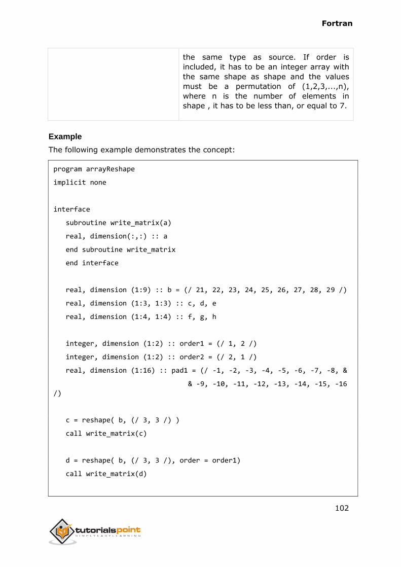
Fortran
102
the same type as source. If order is
included, it has to be an integer array with
the same shape as shape and the values
must be a permutation of (1,2,3,...,n),
where n is the number of elements in
shape , it has to be less than, or equal to 7.
Example
The following example demonstrates the concept:
program arrayReshape
implicit none
interface
subroutine write_matrix(a)
real, dimension(:,:) :: a
end subroutine write_matrix
end interface
real, dimension (1:9) :: b = (/ 21, 22, 23, 24, 25, 26, 27, 28, 29 /)
real, dimension (1:3, 1:3) :: c, d, e
real, dimension (1:4, 1:4) :: f, g, h
integer, dimension (1:2) :: order1 = (/ 1, 2 /)
integer, dimension (1:2) :: order2 = (/ 2, 1 /)
real, dimension (1:16) :: pad1 = (/ -1, -2, -3, -4, -5, -6, -7, -8, &
& -9, -10, -11, -12, -13, -14, -15, -16
/)
c = reshape( b, (/ 3, 3 /) )
call write_matrix(c)
d = reshape( b, (/ 3, 3 /), order = order1)
call write_matrix(d)
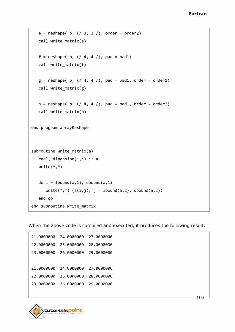
Fortran
103
e = reshape( b, (/ 3, 3 /), order = order2)
call write_matrix(e)
f = reshape( b, (/ 4, 4 /), pad = pad1)
call write_matrix(f)
g = reshape( b, (/ 4, 4 /), pad = pad1, order = order1)
call write_matrix(g)
h = reshape( b, (/ 4, 4 /), pad = pad1, order = order2)
call write_matrix(h)
end program arrayReshape
subroutine write_matrix(a)
real, dimension(:,:) :: a
write(*,*)
do i = lbound(a,1), ubound(a,1)
write(*,*) (a(i,j), j = lbound(a,2), ubound(a,2))
end do
end subroutine write_matrix
When the above code is compiled and executed, it produces the following result:
21.0000000 24.0000000 27.0000000
22.0000000 25.0000000 28.0000000
23.0000000 26.0000000 29.0000000
21.0000000 24.0000000 27.0000000
22.0000000 25.0000000 28.0000000
23.0000000 26.0000000 29.0000000
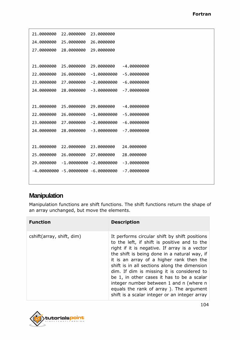
Fortran
104
21.0000000 22.0000000 23.0000000
24.0000000 25.0000000 26.0000000
27.0000000 28.0000000 29.0000000
21.0000000 25.0000000 29.0000000 -4.00000000
22.0000000 26.0000000 -1.00000000 -5.00000000
23.0000000 27.0000000 -2.00000000 -6.00000000
24.0000000 28.0000000 -3.00000000 -7.00000000
21.0000000 25.0000000 29.0000000 -4.00000000
22.0000000 26.0000000 -1.00000000 -5.00000000
23.0000000 27.0000000 -2.00000000 -6.00000000
24.0000000 28.0000000 -3.00000000 -7.00000000
21.0000000 22.0000000 23.0000000 24.0000000
25.0000000 26.0000000 27.0000000 28.0000000
29.0000000 -1.00000000 -2.00000000 -3.00000000
-4.00000000 -5.00000000 -6.00000000 -7.00000000
Manipulation
Manipulation functions are shift functions. The shift functions return the shape of
an array unchanged, but move the elements.
Function Description
cshift(array, shift, dim) It performs circular shift by shift positions
to the left, if shift is positive and to the
right if it is negative. If array is a vector
the shift is being done in a natural way, if
it is an array of a higher rank then the
shift is in all sections along the dimension
dim. If dim is missing it is considered to
be 1, in other cases it has to be a scalar
integer number between 1 and n (where n
equals the rank of array ). The argument
shift is a scalar integer or an integer array
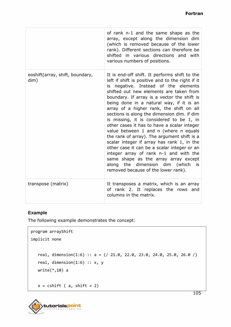
Fortran
105
of rank n-1 and the same shape as the
array, except along the dimension dim
(which is removed because of the lower
rank). Different sections can therefore be
shifted in various directions and with
various numbers of positions.
eoshift(array, shift, boundary,
dim)
It is end-off shift. It performs shift to the
left if shift is positive and to the right if it
is negative. Instead of the elements
shifted out new elements are taken from
boundary. If array is a vector the shift is
being done in a natural way, if it is an
array of a higher rank, the shift on all
sections is along the dimension dim. if dim
is missing, it is considered to be 1, in
other cases it has to have a scalar integer
value between 1 and n (where n equals
the rank of array). The argument shift is a
scalar integer if array has rank 1, in the
other case it can be a scalar integer or an
integer array of rank n-1 and with the
same shape as the array array except
along the dimension dim (which is
removed because of the lower rank).
transpose (matrix) It transposes a matrix, which is an array
of rank 2. It replaces the rows and
columns in the matrix.
Example
The following example demonstrates the concept:
program arrayShift
implicit none
real, dimension(1:6) :: a = (/ 21.0, 22.0, 23.0, 24.0, 25.0, 26.0 /)
real, dimension(1:6) :: x, y
write(*,10) a
x = cshift ( a, shift = 2)
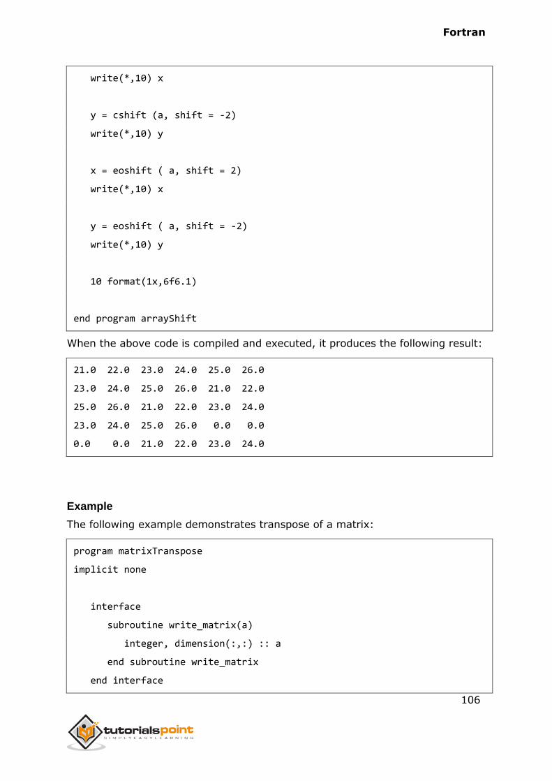
Fortran
106
write(*,10) x
y = cshift (a, shift = -2)
write(*,10) y
x = eoshift ( a, shift = 2)
write(*,10) x
y = eoshift ( a, shift = -2)
write(*,10) y
10 format(1x,6f6.1)
end program arrayShift
When the above code is compiled and executed, it produces the following result:
21.0 22.0 23.0 24.0 25.0 26.0
23.0 24.0 25.0 26.0 21.0 22.0
25.0 26.0 21.0 22.0 23.0 24.0
23.0 24.0 25.0 26.0 0.0 0.0
0.0 0.0 21.0 22.0 23.0 24.0
Example
The following example demonstrates transpose of a matrix:
program matrixTranspose
implicit none
interface
subroutine write_matrix(a)
integer, dimension(:,:) :: a
end subroutine write_matrix
end interface
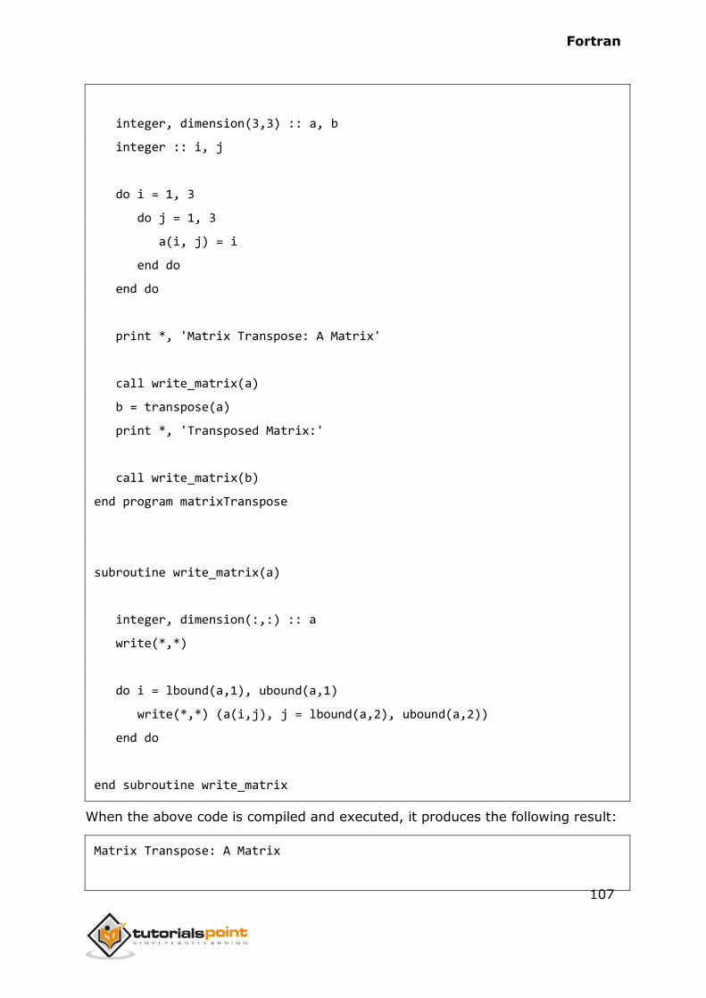
Fortran
107
integer, dimension(3,3) :: a, b
integer :: i, j
do i = 1, 3
do j = 1, 3
a(i, j) = i
end do
end do
print *, 'Matrix Transpose: A Matrix'
call write_matrix(a)
b = transpose(a)
print *, 'Transposed Matrix:'
call write_matrix(b)
end program matrixTranspose
subroutine write_matrix(a)
integer, dimension(:,:) :: a
write(*,*)
do i = lbound(a,1), ubound(a,1)
write(*,*) (a(i,j), j = lbound(a,2), ubound(a,2))
end do
end subroutine write_matrix
When the above code is compiled and executed, it produces the following result:
Matrix Transpose: A Matrix
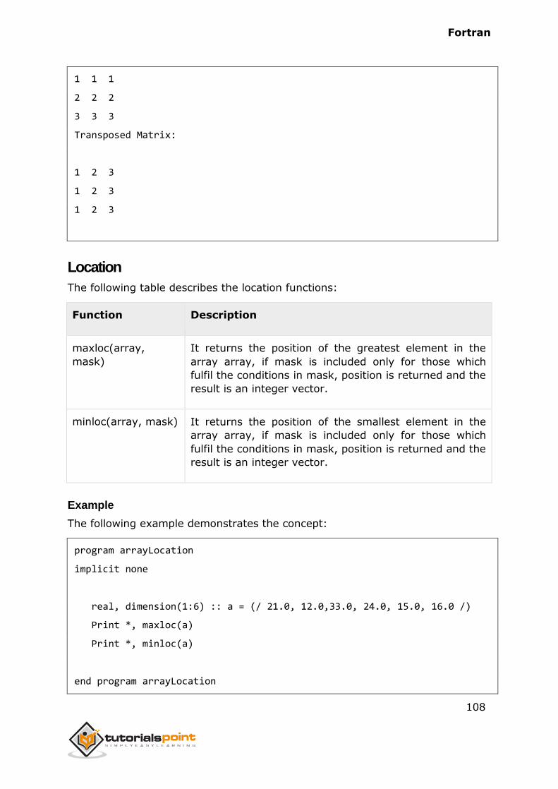
Fortran
108
1 1 1
2 2 2
3 3 3
Transposed Matrix:
1 2 3
1 2 3
1 2 3
Location
The following table describes the location functions:
Function Description
maxloc(array,
mask)
It returns the position of the greatest element in the
array array, if mask is included only for those which
fulfil the conditions in mask, position is returned and the
result is an integer vector.
minloc(array, mask) It returns the position of the smallest element in the
array array, if mask is included only for those which
fulfil the conditions in mask, position is returned and the
result is an integer vector.
Example
The following example demonstrates the concept:
program arrayLocation
implicit none
real, dimension(1:6) :: a = (/ 21.0, 12.0,33.0, 24.0, 15.0, 16.0 /)
Print *, maxloc(a)
Print *, minloc(a)
end program arrayLocation

Fortran
109
When the above code is compiled and executed, it produces the following result:
3
2
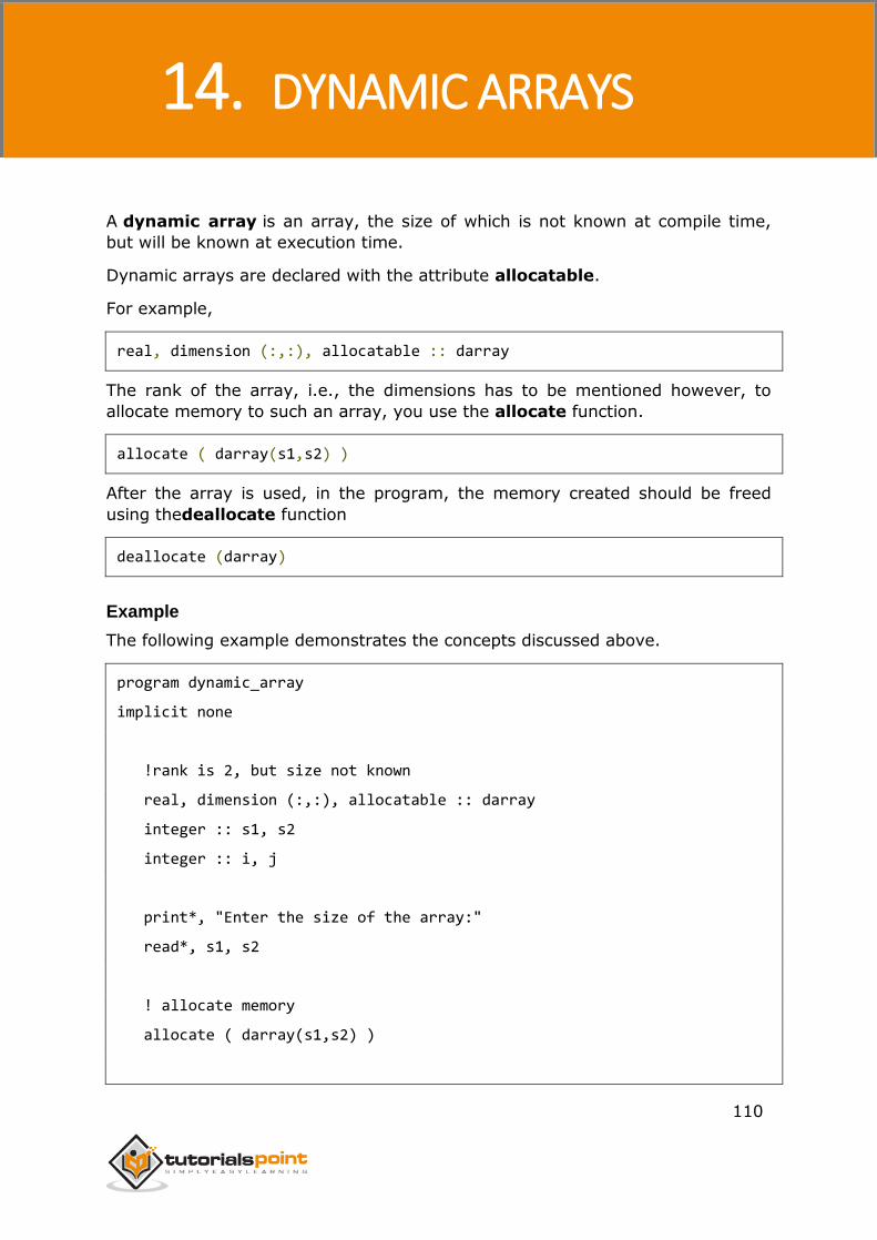
Fortran
110
A dynamic array is an array, the size of which is not known at compile time,
but will be known at execution time.
Dynamic arrays are declared with the attribute allocatable.
For example,
real, dimension (:,:), allocatable :: darray
The rank of the array, i.e., the dimensions has to be mentioned however, to
allocate memory to such an array, you use the allocate function.
allocate ( darray(s1,s2) )
After the array is used, in the program, the memory created should be freed
using thedeallocate function
deallocate (darray)
Example
The following example demonstrates the concepts discussed above.
program dynamic_array
implicit none
!rank is 2, but size not known
real, dimension (:,:), allocatable :: darray
integer :: s1, s2
integer :: i, j
print*, "Enter the size of the array:"
read*, s1, s2
! allocate memory
allocate ( darray(s1,s2) )
14. DYNAMIC ARRAYS
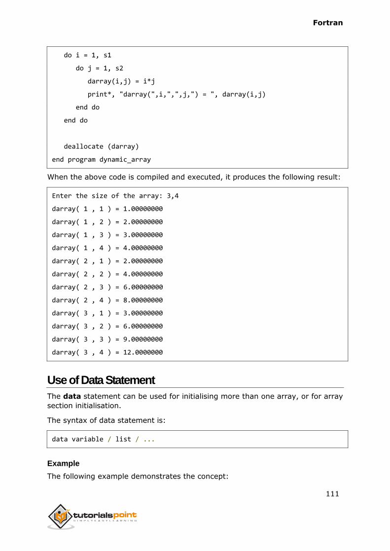
Fortran
111
do i = 1, s1
do j = 1, s2
darray(i,j) = i*j
print*, "darray(",i,",",j,") = ", darray(i,j)
end do
end do
deallocate (darray)
end program dynamic_array
When the above code is compiled and executed, it produces the following result:
Enter the size of the array: 3,4
darray( 1 , 1 ) = 1.00000000
darray( 1 , 2 ) = 2.00000000
darray( 1 , 3 ) = 3.00000000
darray( 1 , 4 ) = 4.00000000
darray( 2 , 1 ) = 2.00000000
darray( 2 , 2 ) = 4.00000000
darray( 2 , 3 ) = 6.00000000
darray( 2 , 4 ) = 8.00000000
darray( 3 , 1 ) = 3.00000000
darray( 3 , 2 ) = 6.00000000
darray( 3 , 3 ) = 9.00000000
darray( 3 , 4 ) = 12.0000000
Use of Data Statement
The data statement can be used for initialising more than one array, or for array
section initialisation.
The syntax of data statement is:
data variable / list / ...
Example
The following example demonstrates the concept:
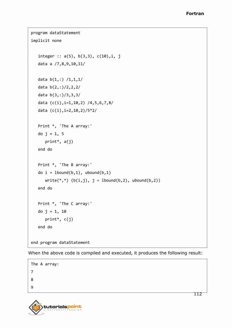
Fortran
112
program dataStatement
implicit none
integer :: a(5), b(3,3), c(10),i, j
data a /7,8,9,10,11/
data b(1,:) /1,1,1/
data b(2,:)/2,2,2/
data b(3,:)/3,3,3/
data (c(i),i=1,10,2) /4,5,6,7,8/
data (c(i),i=2,10,2)/5*2/
Print *, 'The A array:'
do j = 1, 5
print*, a(j)
end do
Print *, 'The B array:'
do i = lbound(b,1), ubound(b,1)
write(*,*) (b(i,j), j = lbound(b,2), ubound(b,2))
end do
Print *, 'The C array:'
do j = 1, 10
print*, c(j)
end do
end program dataStatement
When the above code is compiled and executed, it produces the following result:
The A array:
7
8
9
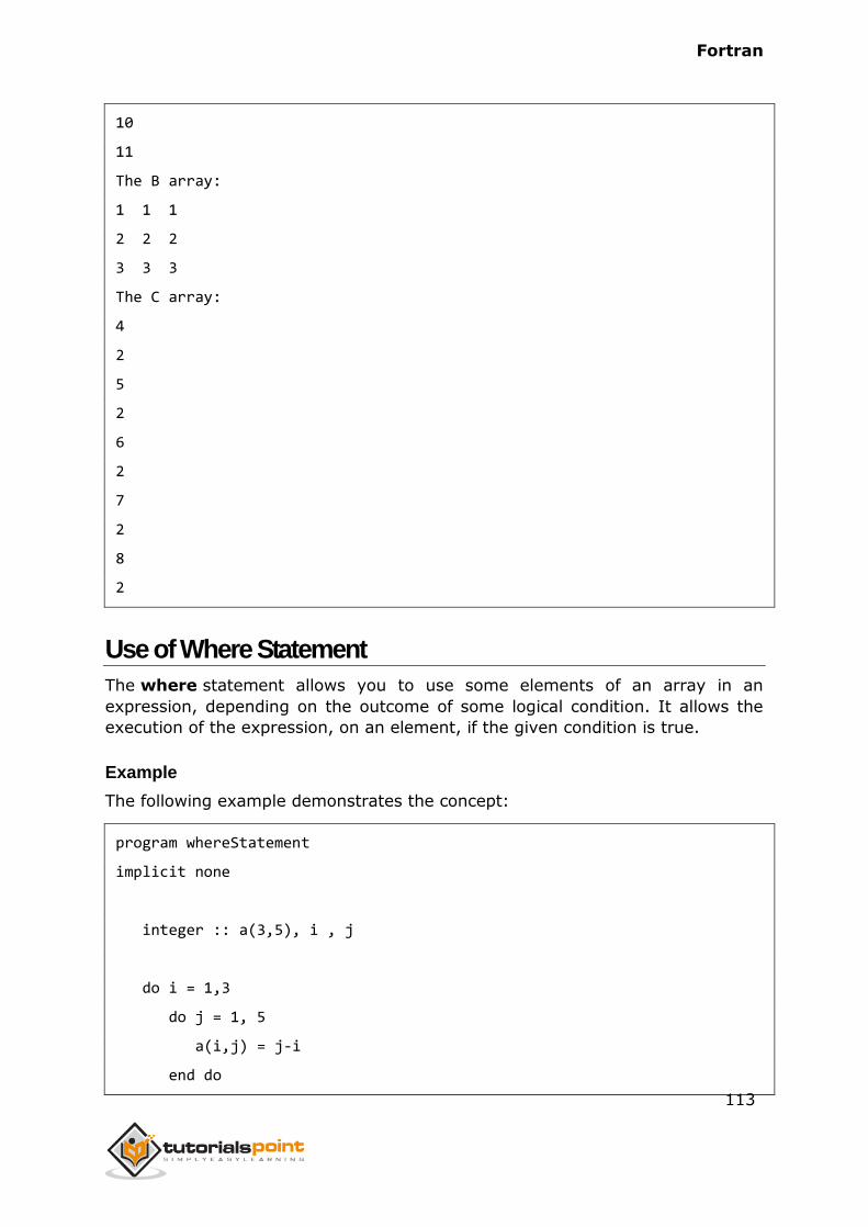
Fortran
113
10
11
The B array:
1 1 1
2 2 2
3 3 3
The C array:
4
2
5
2
6
2
7
2
8
2
Use of Where Statement
The where statement allows you to use some elements of an array in an
expression, depending on the outcome of some logical condition. It allows the
execution of the expression, on an element, if the given condition is true.
Example
The following example demonstrates the concept:
program whereStatement
implicit none
integer :: a(3,5), i , j
do i = 1,3
do j = 1, 5
a(i,j) = j-i
end do
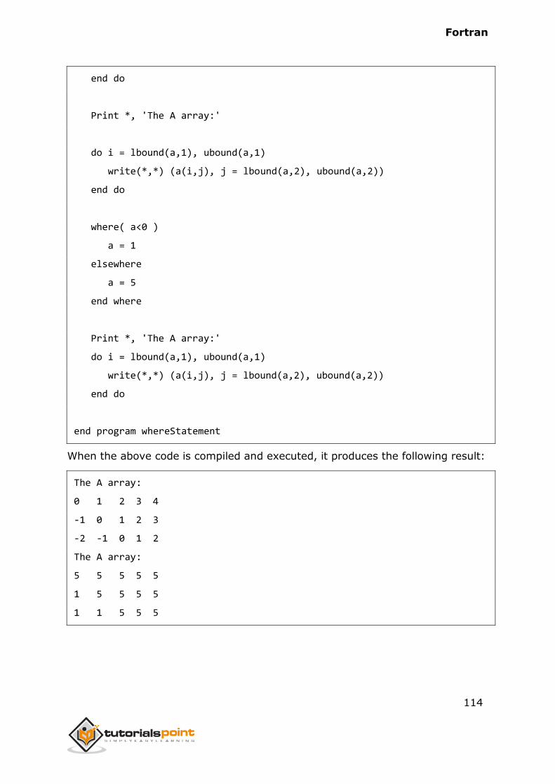
Fortran
114
end do
Print *, 'The A array:'
do i = lbound(a,1), ubound(a,1)
write(*,*) (a(i,j), j = lbound(a,2), ubound(a,2))
end do
where( a<0 )
a = 1
elsewhere
a = 5
end where
Print *, 'The A array:'
do i = lbound(a,1), ubound(a,1)
write(*,*) (a(i,j), j = lbound(a,2), ubound(a,2))
end do
end program whereStatement
When the above code is compiled and executed, it produces the following result:
The A array:
0 1 2 3 4
-1 0 1 2 3
-2 -1 0 1 2
The A array:
5 5 5 5 5
1 5 5 5 5
1 1 5 5 5
Fortran
115
Fortran allows you to define derived data types. A derived data type is also
called a structure, and it can consist of data objects of different types.
Derived data types are used to represent a record. E.g. you want to keep track
of your books in a library, you might want to track the following attributes about
each book:
Title
Author
Subject
Book ID
Defining a Derived data type
To define a derived data type, the type and end type statements are used. .
The type statement defines a new data type, with more than one member for
your program. The format of the type statement is this:
type type_name
declarations
end type
Here is the way you would declare the Book structure:
type Books
character(len=50) :: title
character(len=50) :: author
character(len=150) :: subject
integer :: book_id
end type Books
Accessing Structure Members
An object of a derived data type is called a structure
A structure of type Books can be created in a type declaration statement like:
15. DERIVED DATA TYPES
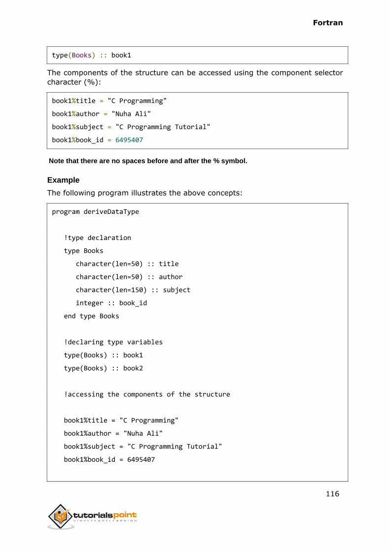
Fortran
116
type(Books) :: book1
The components of the structure can be accessed using the component selector
character (%):
book1%title = "C Programming"
book1%author = "Nuha Ali"
book1%subject = "C Programming Tutorial"
book1%book_id = 6495407
Note that there are no spaces before and after the % symbol.
Example
The following program illustrates the above concepts:
program deriveDataType
!type declaration
type Books
character(len=50) :: title
character(len=50) :: author
character(len=150) :: subject
integer :: book_id
end type Books
!declaring type variables
type(Books) :: book1
type(Books) :: book2
!accessing the components of the structure
book1%title = "C Programming"
book1%author = "Nuha Ali"
book1%subject = "C Programming Tutorial"
book1%book_id = 6495407

Fortran
117
book2%title = "Telecom Billing"
book2%author = "Zara Ali"
book2%subject = "Telecom Billing Tutorial"
book2%book_id = 6495700
!display book info
Print *, book1%title
Print *, book1%author
Print *, book1%subject
Print *, book1%book_id
Print *, book2%title
Print *, book2%author
Print *, book2%subject
Print *, book2%book_id
end program deriveDataType
When the above code is compiled and executed, it produces the following result:
C Programming
Nuha Ali
C Programming Tutorial
6495407
Telecom Billing
Zara Ali
Telecom Billing Tutorial
6495700
Array of Structures
You can also create arrays of a derived type:
type(Books), dimension(2) :: list
Individual elements of the array could be accessed as:
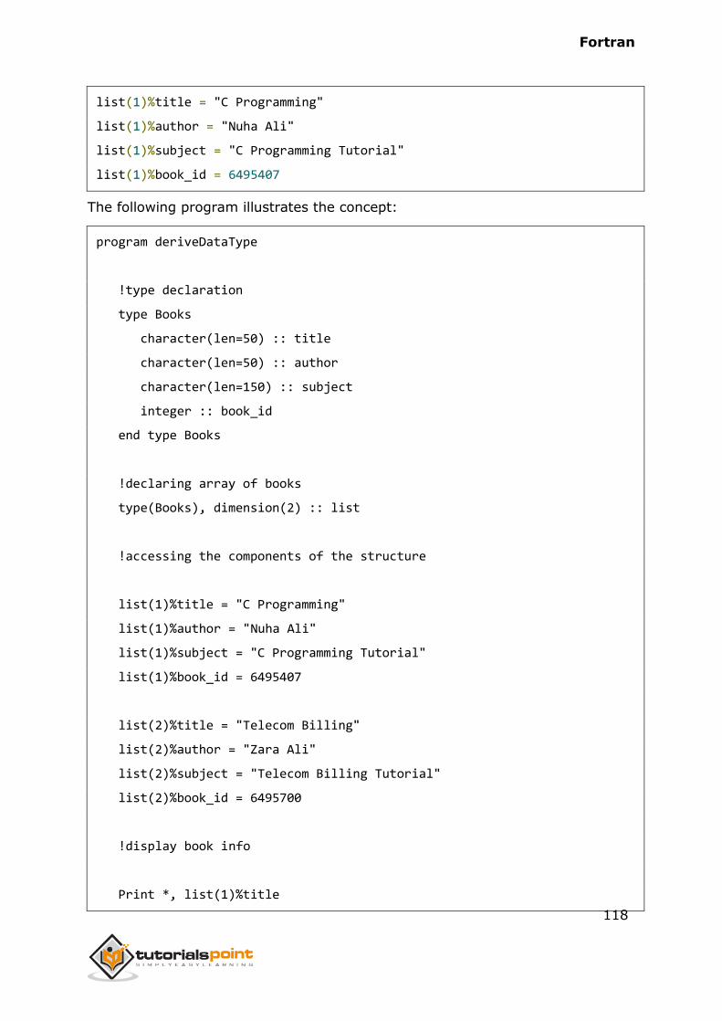
Fortran
118
list(1)%title = "C Programming"
list(1)%author = "Nuha Ali"
list(1)%subject = "C Programming Tutorial"
list(1)%book_id = 6495407
The following program illustrates the concept:
program deriveDataType
!type declaration
type Books
character(len=50) :: title
character(len=50) :: author
character(len=150) :: subject
integer :: book_id
end type Books
!declaring array of books
type(Books), dimension(2) :: list
!accessing the components of the structure
list(1)%title = "C Programming"
list(1)%author = "Nuha Ali"
list(1)%subject = "C Programming Tutorial"
list(1)%book_id = 6495407
list(2)%title = "Telecom Billing"
list(2)%author = "Zara Ali"
list(2)%subject = "Telecom Billing Tutorial"
list(2)%book_id = 6495700
!display book info
Print *, list(1)%title
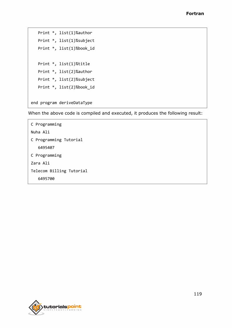
Fortran
119
Print *, list(1)%author
Print *, list(1)%subject
Print *, list(1)%book_id
Print *, list(1)%title
Print *, list(2)%author
Print *, list(2)%subject
Print *, list(2)%book_id
end program deriveDataType
When the above code is compiled and executed, it produces the following result:
C Programming
Nuha Ali
C Programming Tutorial
6495407
C Programming
Zara Ali
Telecom Billing Tutorial
6495700
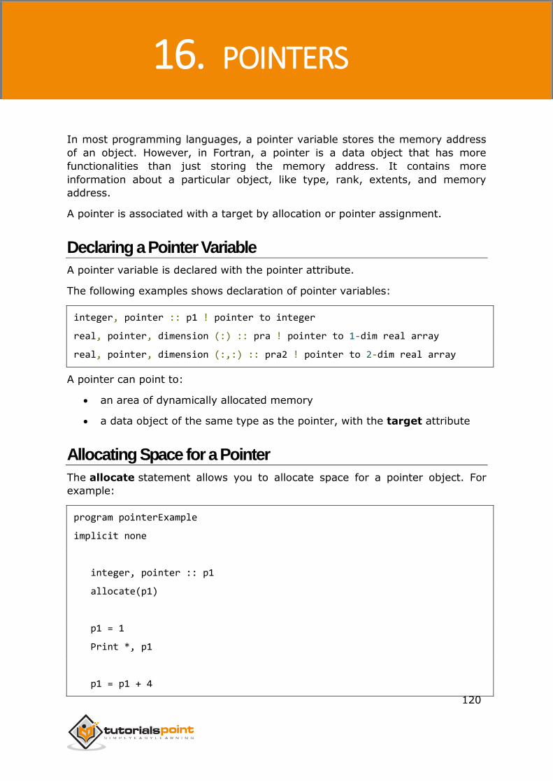
Fortran
120
In most programming languages, a pointer variable stores the memory address
of an object. However, in Fortran, a pointer is a data object that has more
functionalities than just storing the memory address. It contains more
information about a particular object, like type, rank, extents, and memory
address.
A pointer is associated with a target by allocation or pointer assignment.
Declaring a Pointer Variable
A pointer variable is declared with the pointer attribute.
The following examples shows declaration of pointer variables:
integer, pointer :: p1 ! pointer to integer
real, pointer, dimension (:) :: pra ! pointer to 1-dim real array
real, pointer, dimension (:,:) :: pra2 ! pointer to 2-dim real array
A pointer can point to:
an area of dynamically allocated memory
a data object of the same type as the pointer, with the target attribute
Allocating Space for a Pointer
The allocate statement allows you to allocate space for a pointer object. For
example:
program pointerExample
implicit none
integer, pointer :: p1
allocate(p1)
p1 = 1
Print *, p1
p1 = p1 + 4
16. POINTERS
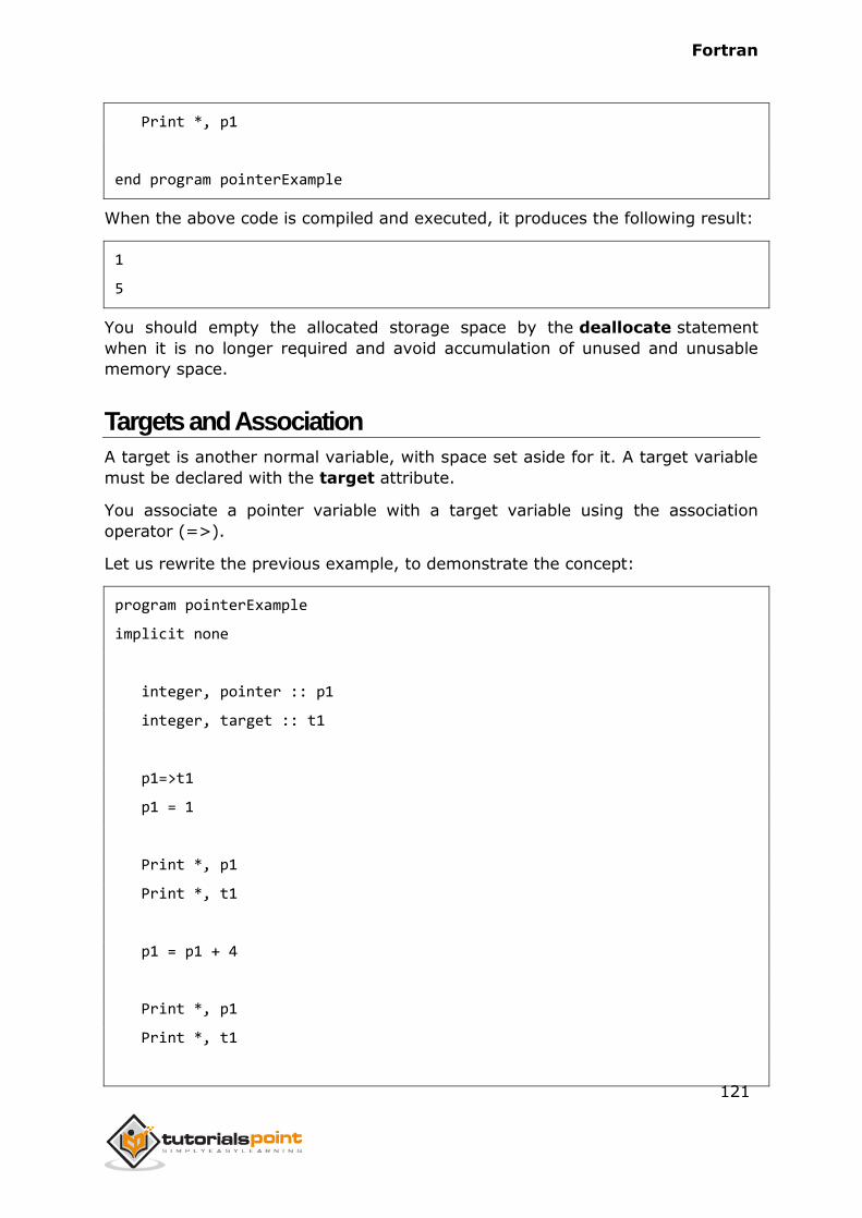
Fortran
121
Print *, p1
end program pointerExample
When the above code is compiled and executed, it produces the following result:
1
5
You should empty the allocated storage space by the deallocate statement
when it is no longer required and avoid accumulation of unused and unusable
memory space.
Targets and Association
A target is another normal variable, with space set aside for it. A target variable
must be declared with the target attribute.
You associate a pointer variable with a target variable using the association
operator (=>).
Let us rewrite the previous example, to demonstrate the concept:
program pointerExample
implicit none
integer, pointer :: p1
integer, target :: t1
p1=>t1
p1 = 1
Print *, p1
Print *, t1
p1 = p1 + 4
Print *, p1
Print *, t1
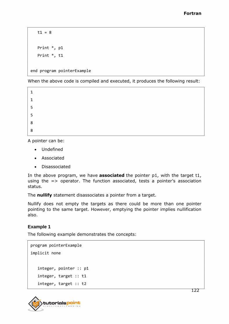
Fortran
122
t1 = 8
Print *, p1
Print *, t1
end program pointerExample
When the above code is compiled and executed, it produces the following result:
1
1
5
5
8
8
A pointer can be:
Undefined
Associated
Disassociated
In the above program, we have associated the pointer p1, with the target t1,
using the => operator. The function associated, tests a pointer’s association
status.
The nullify statement disassociates a pointer from a target.
Nullify does not empty the targets as there could be more than one pointer
pointing to the same target. However, emptying the pointer implies nullification
also.
Example 1
The following example demonstrates the concepts:
program pointerExample
implicit none
integer, pointer :: p1
integer, target :: t1
integer, target :: t2
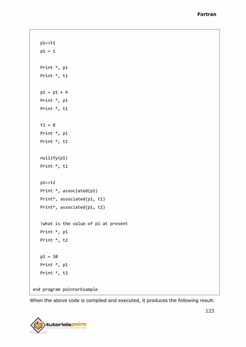
Fortran
123
p1=>t1
p1 = 1
Print *, p1
Print *, t1
p1 = p1 + 4
Print *, p1
Print *, t1
t1 = 8
Print *, p1
Print *, t1
nullify(p1)
Print *, t1
p1=>t2
Print *, associated(p1)
Print*, associated(p1, t1)
Print*, associated(p1, t2)
!what is the value of p1 at present
Print *, p1
Print *, t2
p1 = 10
Print *, p1
Print *, t2
end program pointerExample
When the above code is compiled and executed, it produces the following result:
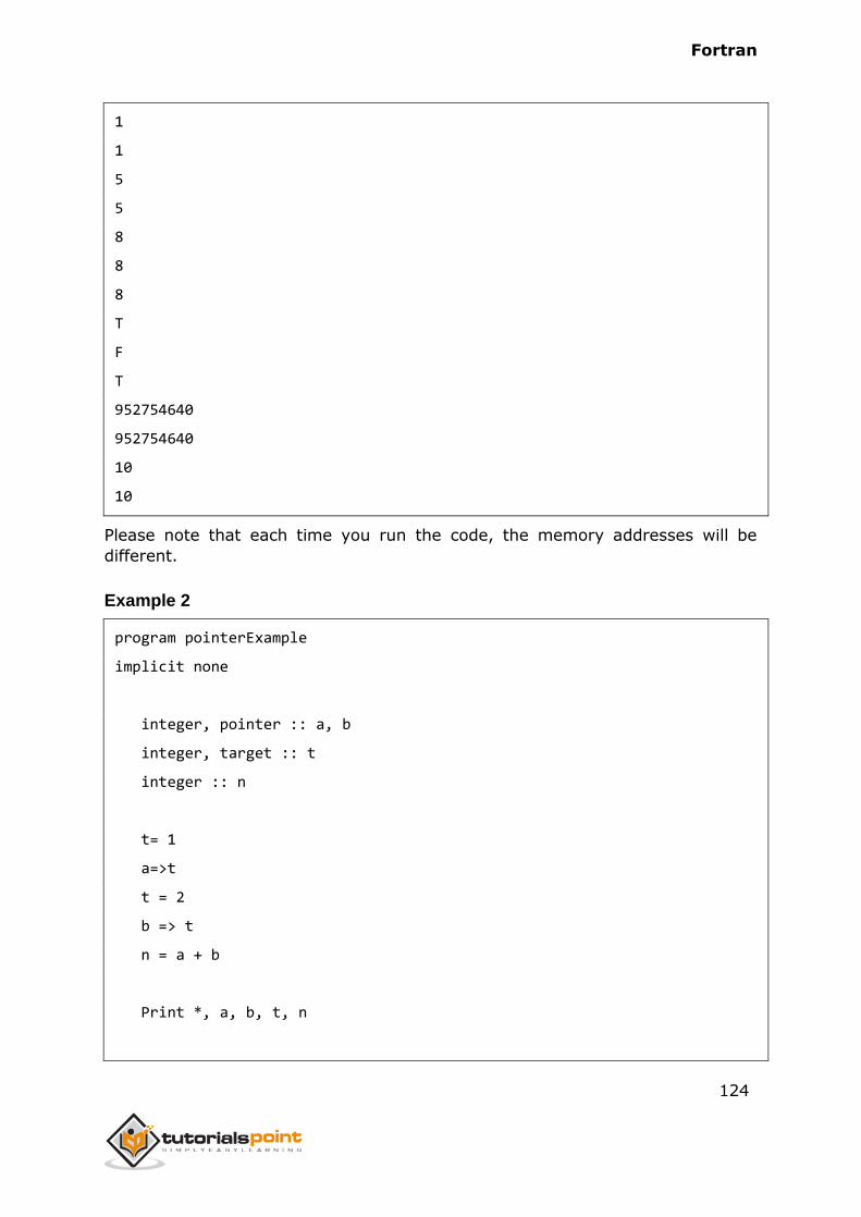
Fortran
124
1
1
5
5
8
8
8
T
F
T
952754640
952754640
10
10
Please note that each time you run the code, the memory addresses will be
different.
Example 2
program pointerExample
implicit none
integer, pointer :: a, b
integer, target :: t
integer :: n
t= 1
a=>t
t = 2
b => t
n = a + b
Print *, a, b, t, n
Fortran
125
end program pointerExample
When the above code is compiled and executed, it produces the following result:
2 2 2 4
Fortran
126
We have so far seen that we can read data from keyboard using the read
* statement, and display output to the screen using the print* statement,
respectively. This form of input-output is free format I/O, and it is called list-
directed input-output.
The free format simple I/O has the form:
read(*,*) item1, item2, item3...
print *, item1, item2, item3
write(*,*) item1, item2, item3...
However the formatted I/O gives you more flexibility over data transfer.
Formatted Input Output
Formatted input output has the syntax as follows:
read fmt, variable_list
print fmt, variable_list
write fmt, variable_list
Where,
fmt is the format specification
variable-list is a list of the variables to be read from keyboard or written
on screen
Format specification defines the way in which formatted data is displayed. It
consists of a string, containing a list of edit descriptors in parentheses.
An edit descriptor specifies the exact format, for example, width, digits after
decimal point etc., in which characters and numbers are displayed.
For example:
Print "(f6.3)", pi
17. BASIC INPUT OUTPUT
Fortran
127
The following table describes the descriptors:
Descriptor Description Example
I This is used for integer output.
This takes the form ‘rIw.m’
where the meanings of r, w and
m are given in the table below.
Integer values are right justified
in their fields. If the field width
is not large enough to
accommodate an integer then
the field is filled with asterisks.
print "(3i5)", i, j, k
F This is used for real number
output. This takes the form
‘rFw.d’ where the meanings of r,
w and d are given in the table
below. Real values are right
justified in their fields. If the
field width is not large enough
to accommodate the real
number then the field is filled
with asterisks.
print "(f12.3)",pi
E This is used for real output in
exponential notation. The ‘E’
descriptor statement takes the
form ‘rEw.d’ where the
meanings of r, w and d are
given in the table below. Real
values are right justified in their
fields. If the field width is not
large enough to accommodate
the real number then the field is
filled with asterisks.
Please note that, to print out a
real number with three decimal
places a field width of at least
ten is needed. One for the sign
of the mantissa, two for the
zero, four for the mantissa and
two for the exponent itself. In
print "(e10.3)",123456.0 gives
‘0.123e+06’
Fortran
128
general, w ≥ d + 7.
ES This is used for real output
(scientific notation). This takes
the form ‘rESw.d’ where the
meanings of r, w and d are
given in the table below. The ‘E’
descriptor described above
differs slightly from the
traditional well known ‘scientific
notation’. Scientific notation has
the mantissa in the range 1.0 to
10.0 unlike the E descriptor
which has the mantissa in the
range 0.1 to 1.0. Real values
are right justified in their fields.
If the field width is not large
enough to accommodate the
real number then the field is
filled with asterisks. Here also,
the width field must satisfy the
expression w ≥ d + 7
print "(es10.3)",123456.0
gives ‘1.235e+05’
A This is used for character
output. This takes the form
‘rAw’ where the meanings of r
and w are given in the table
below. Character types are right
justified in their fields. If the
field width is not large enough
to accommodate the character
string then the field is filled with
the first ‘w’ characters of the
string.
print "(a10)", str
X This is used for space output.
This takes the form ‘nX’ where
‘n’ is the number of desired
spaces.
print "(5x, a10)", str
/ Slash descriptor – used to insert
blank lines. This takes the form
‘/’ and forces the next data
print "(/,5x, a10)", str
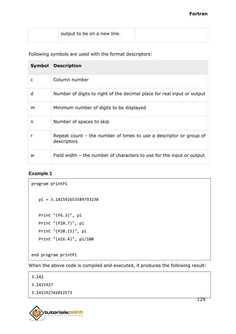
Fortran
129
output to be on a new line.
Following symbols are used with the format descriptors:
Symbol Description
c Column number
d Number of digits to right of the decimal place for real input or output
m Minimum number of digits to be displayed
n Number of spaces to skip
r Repeat count – the number of times to use a descriptor or group of
descriptors
w Field width – the number of characters to use for the input or output
Example 1
program printPi
pi = 3.141592653589793238
Print "(f6.3)", pi
Print "(f10.7)", pi
Print "(f20.15)", pi
Print "(e16.4)", pi/100
end program printPi
When the above code is compiled and executed, it produces the following result:
3.142
3.1415927
3.141592741012573
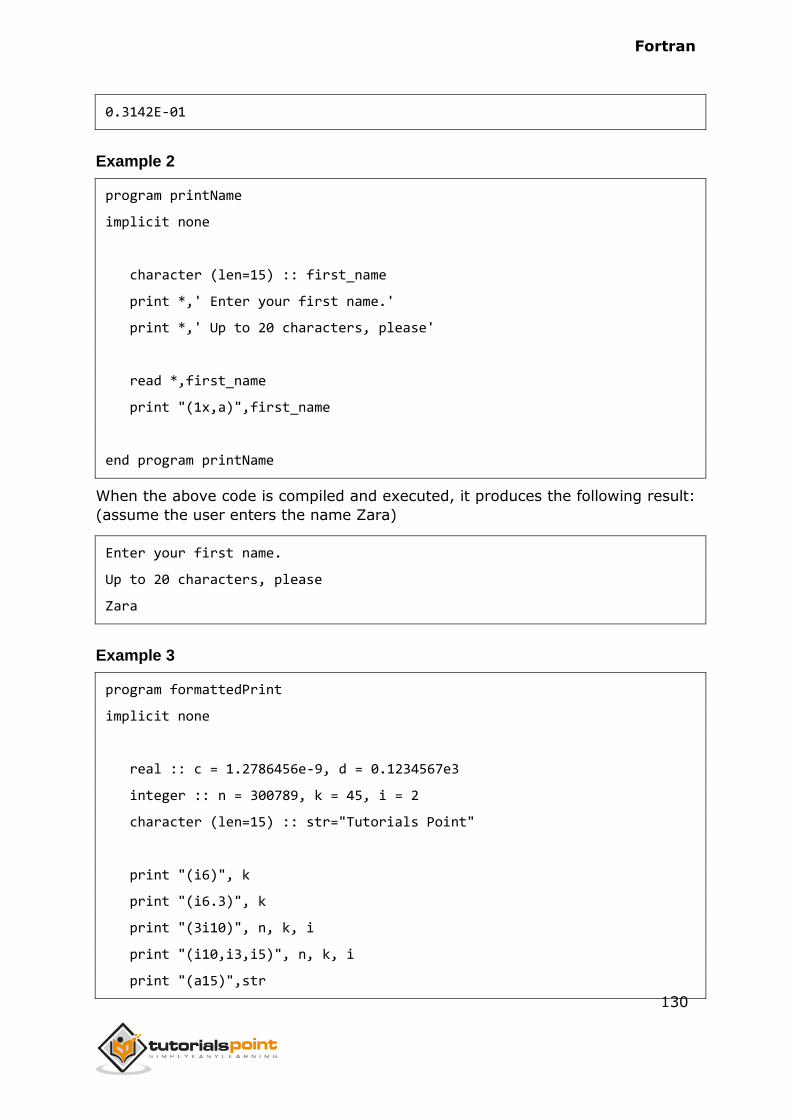
Fortran
130
0.3142E-01
Example 2
program printName
implicit none
character (len=15) :: first_name
print *,' Enter your first name.'
print *,' Up to 20 characters, please'
read *,first_name
print "(1x,a)",first_name
end program printName
When the above code is compiled and executed, it produces the following result:
(assume the user enters the name Zara)
Enter your first name.
Up to 20 characters, please
Zara
Example 3
program formattedPrint
implicit none
real :: c = 1.2786456e-9, d = 0.1234567e3
integer :: n = 300789, k = 45, i = 2
character (len=15) :: str="Tutorials Point"
print "(i6)", k
print "(i6.3)", k
print "(3i10)", n, k, i
print "(i10,i3,i5)", n, k, i
print "(a15)",str
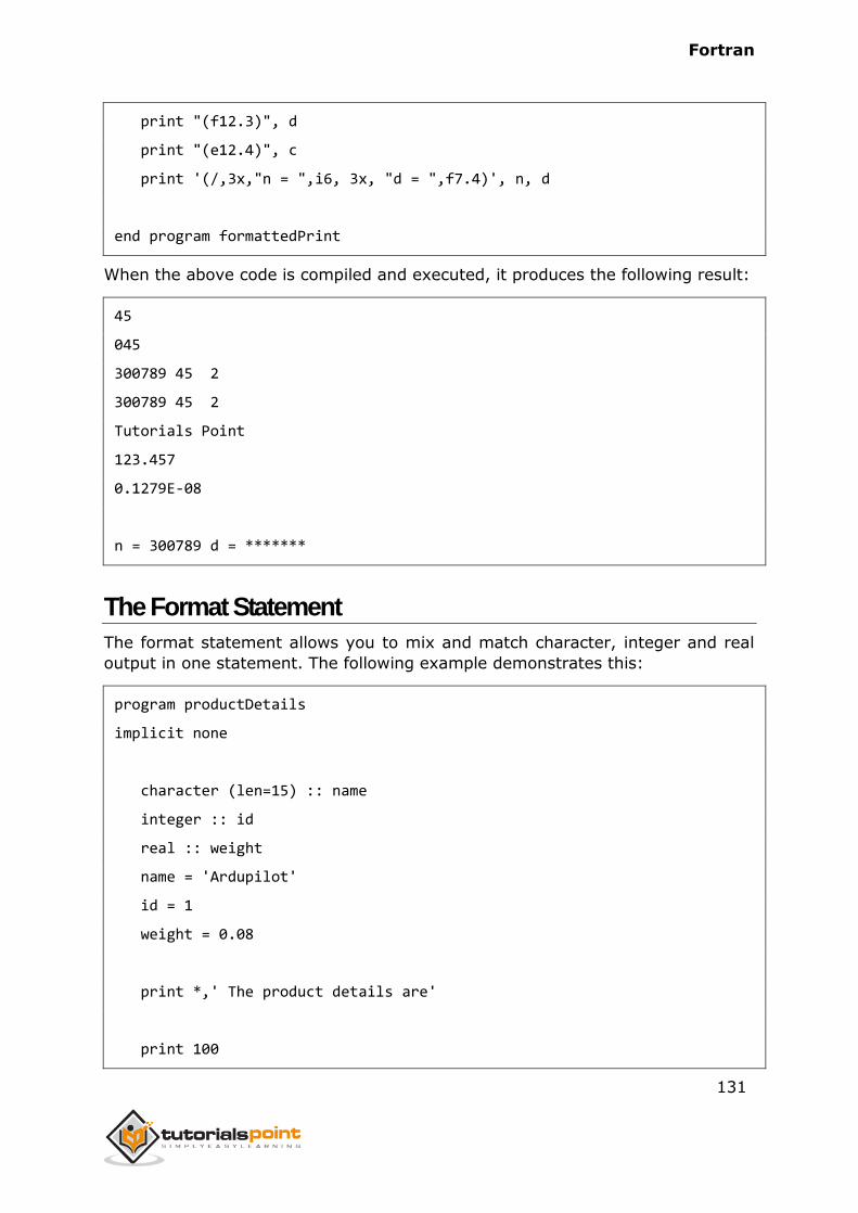
Fortran
131
print "(f12.3)", d
print "(e12.4)", c
print '(/,3x,"n = ",i6, 3x, "d = ",f7.4)', n, d
end program formattedPrint
When the above code is compiled and executed, it produces the following result:
45
045
300789 45 2
300789 45 2
Tutorials Point
123.457
0.1279E-08
n = 300789 d = *******
The Format Statement
The format statement allows you to mix and match character, integer and real
output in one statement. The following example demonstrates this:
program productDetails
implicit none
character (len=15) :: name
integer :: id
real :: weight
name = 'Ardupilot'
id = 1
weight = 0.08
print *,' The product details are'
print 100
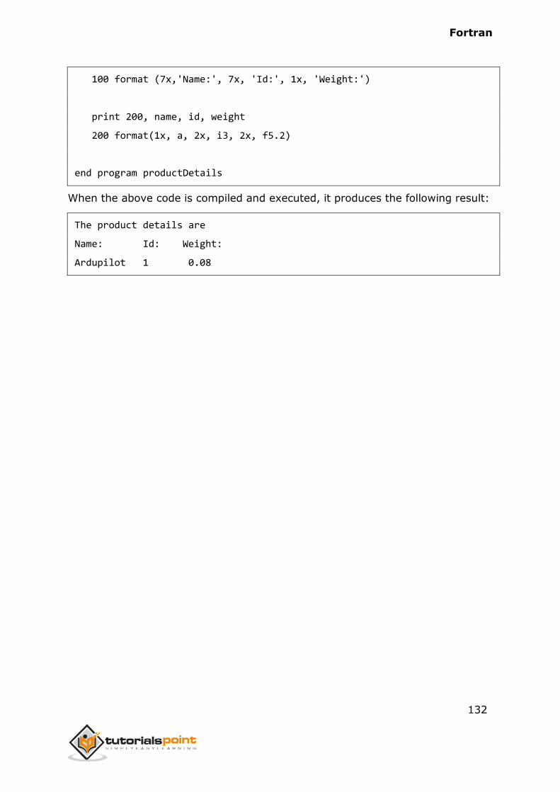
Fortran
132
100 format (7x,'Name:', 7x, 'Id:', 1x, 'Weight:')
print 200, name, id, weight
200 format(1x, a, 2x, i3, 2x, f5.2)
end program productDetails
When the above code is compiled and executed, it produces the following result:
The product details are
Name: Id: Weight:
Ardupilot 1 0.08
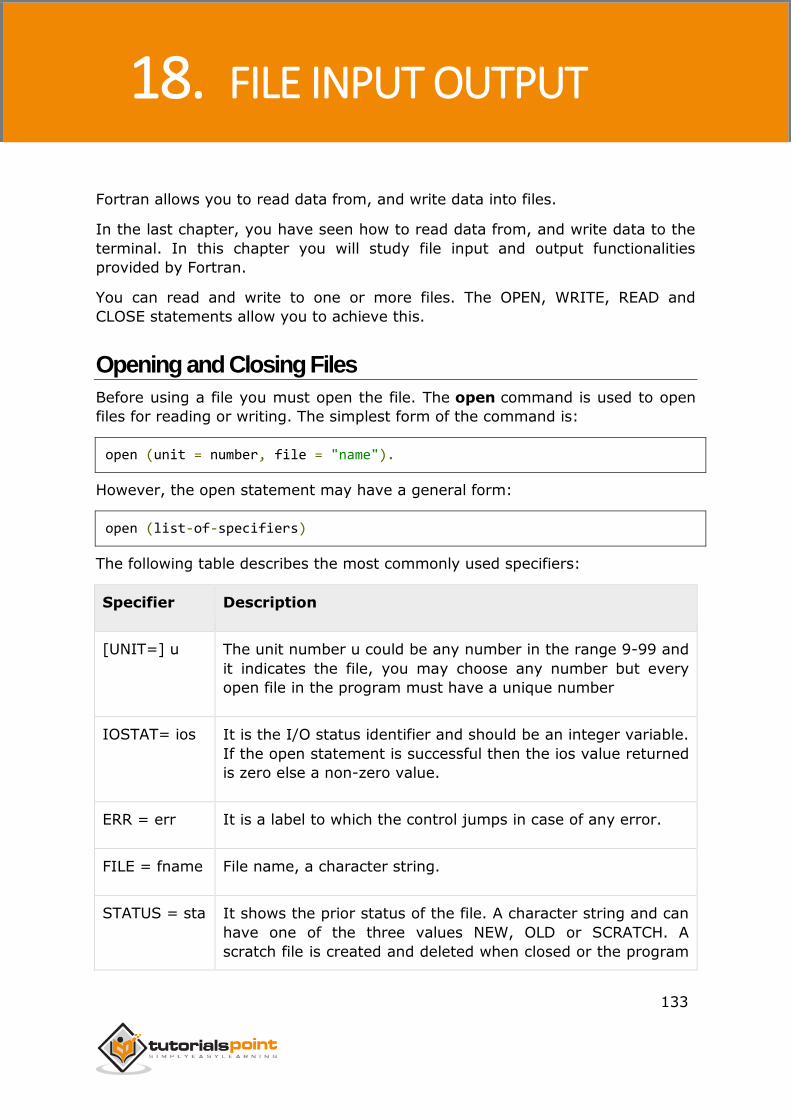
Fortran
133
Fortran allows you to read data from, and write data into files.
In the last chapter, you have seen how to read data from, and write data to the
terminal. In this chapter you will study file input and output functionalities
provided by Fortran.
You can read and write to one or more files. The OPEN, WRITE, READ and
CLOSE statements allow you to achieve this.
Opening and Closing Files
Before using a file you must open the file. The open command is used to open
files for reading or writing. The simplest form of the command is:
open (unit = number, file = "name").
However, the open statement may have a general form:
open (list-of-specifiers)
The following table describes the most commonly used specifiers:
Specifier Description
[UNIT=] u The unit number u could be any number in the range 9-99 and
it indicates the file, you may choose any number but every
open file in the program must have a unique number
IOSTAT= ios It is the I/O status identifier and should be an integer variable.
If the open statement is successful then the ios value returned
is zero else a non-zero value.
ERR = err It is a label to which the control jumps in case of any error.
FILE = fname File name, a character string.
STATUS = sta It shows the prior status of the file. A character string and can
have one of the three values NEW, OLD or SCRATCH. A
scratch file is created and deleted when closed or the program
18. FILE INPUT OUTPUT
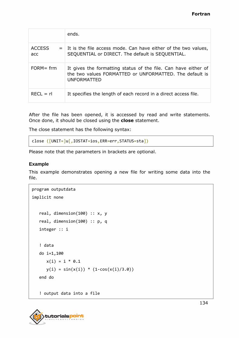
Fortran
134
ends.
ACCESS =
acc
It is the file access mode. Can have either of the two values,
SEQUENTIAL or DIRECT. The default is SEQUENTIAL.
FORM= frm It gives the formatting status of the file. Can have either of
the two values FORMATTED or UNFORMATTED. The default is
UNFORMATTED
RECL = rl It specifies the length of each record in a direct access file.
After the file has been opened, it is accessed by read and write statements.
Once done, it should be closed using the close statement.
The close statement has the following syntax:
close ([UNIT=]u[,IOSTAT=ios,ERR=err,STATUS=sta])
Please note that the parameters in brackets are optional.
Example
This example demonstrates opening a new file for writing some data into the
file.
program outputdata
implicit none
real, dimension(100) :: x, y
real, dimension(100) :: p, q
integer :: i
! data
do i=1,100
x(i) = i * 0.1
y(i) = sin(x(i)) * (1-cos(x(i)/3.0))
end do
! output data into a file

Fortran
135
open(1, file='data1.dat', status='new')
do i=1,100
write(1,*) x(i), y(i)
end do
close(1)
end program outputdata
When the above code is compiled and executed, it creates the file data1.dat and
writes the x and y array values into it. And then closes the file.
Reading from and Writing into the File
The read and write statements respectively are used for reading from and
writing into a file respectively.
They have the following syntax:
read ([UNIT=]u, [FMT=]fmt, IOSTAT=ios, ERR=err, END=s)
write([UNIT=]u, [FMT=]fmt, IOSTAT=ios, ERR=err, END=s)
Most of the specifiers have already been discussed in the above table.
The END=s specifier is a statement label where the program jumps, when it
reaches end-of-file.
Example
This example demonstrates reading from and writing into a file.
In this program we read from the file, we created in the last example, data1.dat,
and display it on screen.
program outputdata
implicit none
real, dimension(100) :: x, y
real, dimension(100) :: p, q
integer :: i
! data
do i=1,100
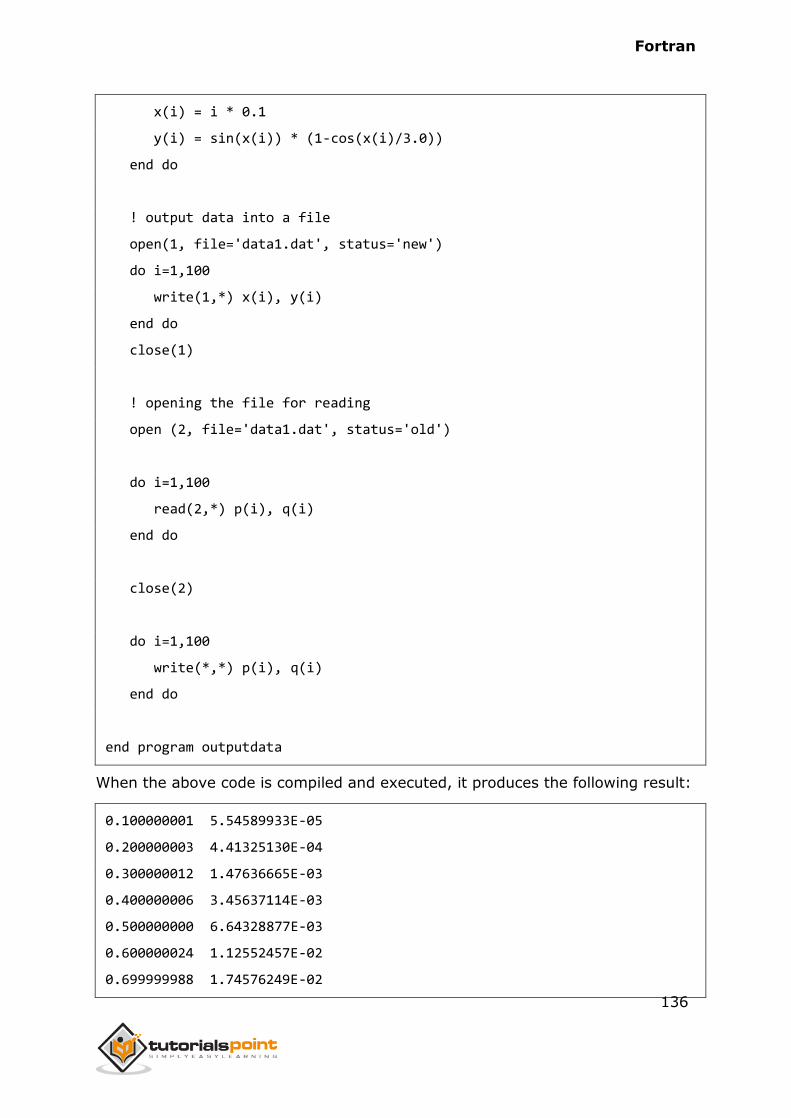
Fortran
136
x(i) = i * 0.1
y(i) = sin(x(i)) * (1-cos(x(i)/3.0))
end do
! output data into a file
open(1, file='data1.dat', status='new')
do i=1,100
write(1,*) x(i), y(i)
end do
close(1)
! opening the file for reading
open (2, file='data1.dat', status='old')
do i=1,100
read(2,*) p(i), q(i)
end do
close(2)
do i=1,100
write(*,*) p(i), q(i)
end do
end program outputdata
When the above code is compiled and executed, it produces the following result:
0.100000001 5.54589933E-05
0.200000003 4.41325130E-04
0.300000012 1.47636665E-03
0.400000006 3.45637114E-03
0.500000000 6.64328877E-03
0.600000024 1.12552457E-02
0.699999988 1.74576249E-02
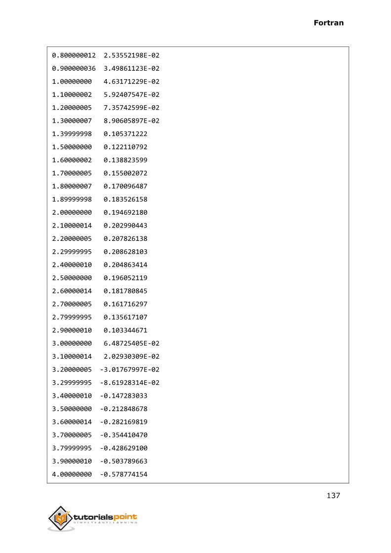
Fortran
137
0.800000012 2.53552198E-02
0.900000036 3.49861123E-02
1.00000000 4.63171229E-02
1.10000002 5.92407547E-02
1.20000005 7.35742599E-02
1.30000007 8.90605897E-02
1.39999998 0.105371222
1.50000000 0.122110792
1.60000002 0.138823599
1.70000005 0.155002072
1.80000007 0.170096487
1.89999998 0.183526158
2.00000000 0.194692180
2.10000014 0.202990443
2.20000005 0.207826138
2.29999995 0.208628103
2.40000010 0.204863414
2.50000000 0.196052119
2.60000014 0.181780845
2.70000005 0.161716297
2.79999995 0.135617107
2.90000010 0.103344671
3.00000000 6.48725405E-02
3.10000014 2.02930309E-02
3.20000005 -3.01767997E-02
3.29999995 -8.61928314E-02
3.40000010 -0.147283033
3.50000000 -0.212848678
3.60000014 -0.282169819
3.70000005 -0.354410470
3.79999995 -0.428629100
3.90000010 -0.503789663
4.00000000 -0.578774154
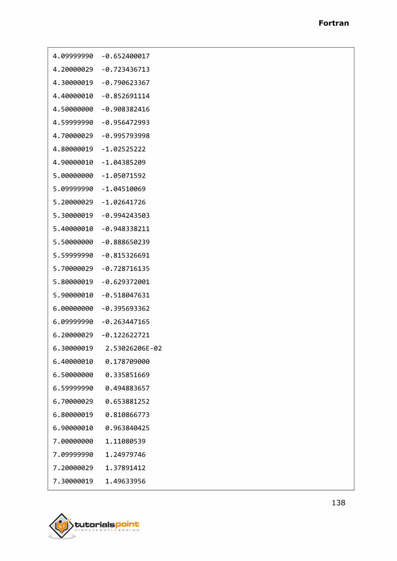
Fortran
138
4.09999990 -0.652400017
4.20000029 -0.723436713
4.30000019 -0.790623367
4.40000010 -0.852691114
4.50000000 -0.908382416
4.59999990 -0.956472993
4.70000029 -0.995793998
4.80000019 -1.02525222
4.90000010 -1.04385209
5.00000000 -1.05071592
5.09999990 -1.04510069
5.20000029 -1.02641726
5.30000019 -0.994243503
5.40000010 -0.948338211
5.50000000 -0.888650239
5.59999990 -0.815326691
5.70000029 -0.728716135
5.80000019 -0.629372001
5.90000010 -0.518047631
6.00000000 -0.395693362
6.09999990 -0.263447165
6.20000029 -0.122622721
6.30000019 2.53026206E-02
6.40000010 0.178709000
6.50000000 0.335851669
6.59999990 0.494883657
6.70000029 0.653881252
6.80000019 0.810866773
6.90000010 0.963840425
7.00000000 1.11080539
7.09999990 1.24979746
7.20000029 1.37891412
7.30000019 1.49633956
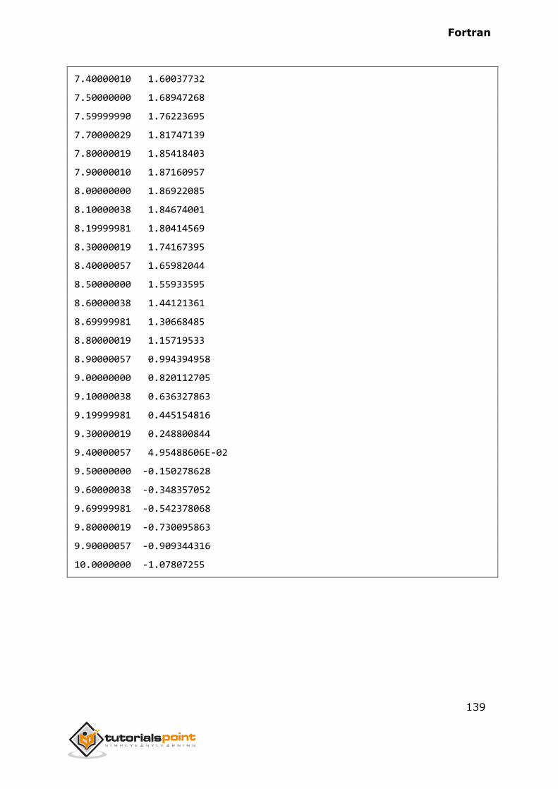
Fortran
139
7.40000010 1.60037732
7.50000000 1.68947268
7.59999990 1.76223695
7.70000029 1.81747139
7.80000019 1.85418403
7.90000010 1.87160957
8.00000000 1.86922085
8.10000038 1.84674001
8.19999981 1.80414569
8.30000019 1.74167395
8.40000057 1.65982044
8.50000000 1.55933595
8.60000038 1.44121361
8.69999981 1.30668485
8.80000019 1.15719533
8.90000057 0.994394958
9.00000000 0.820112705
9.10000038 0.636327863
9.19999981 0.445154816
9.30000019 0.248800844
9.40000057 4.95488606E-02
9.50000000 -0.150278628
9.60000038 -0.348357052
9.69999981 -0.542378068
9.80000019 -0.730095863
9.90000057 -0.909344316
10.0000000 -1.07807255
Fortran
140
A procedure is a group of statements that perform a well-defined task and can
be invoked from your program. Information (or data) is passed to the calling
program, to the procedure as arguments.
There are two types of procedures:
Functions
Subroutines
Function
A function is a procedure that returns a single quantity. A function should not
modify its arguments.
The returned quantity is known as function value, and it is denoted by the
function name.
Syntax:
Syntax for a function is as follows:
function name(arg1, arg2, ....)
[declarations, including those for the arguments]
[executable statements]
end function [name]
The following example demonstrates a function named area_of_circle. It
calculates the area of a circle with radius r.
program calling_func
real :: a
a = area_of_circle(2.0)
Print *, "The area of a circle with radius 2.0 is"
Print *, a
end program calling_func
19. PROCEDURES
Fortran
141
! this function computes the area of a circle with radius r
function area_of_circle (r)
! function result
implicit none
! dummy arguments
real :: area_of_circle
! local variables
real :: r
real :: pi
pi = 4 * atan (1.0)
area_of_circle = pi * r**2
end function area_of_circle
When you compile and execute the above program, it produces the following
result:
The area of a circle with radius 2.0 is
12.5663710
Please note that:
You must specify implicit none in both the main program as well as the
procedure.
The argument r in the called function is called dummy argument.
The result Option
If you want the returned value to be stored in some other name than the
function name, you can use the result option.
You can specify the return variable name as:
function name(arg1, arg2, ....) result (return_var_name)
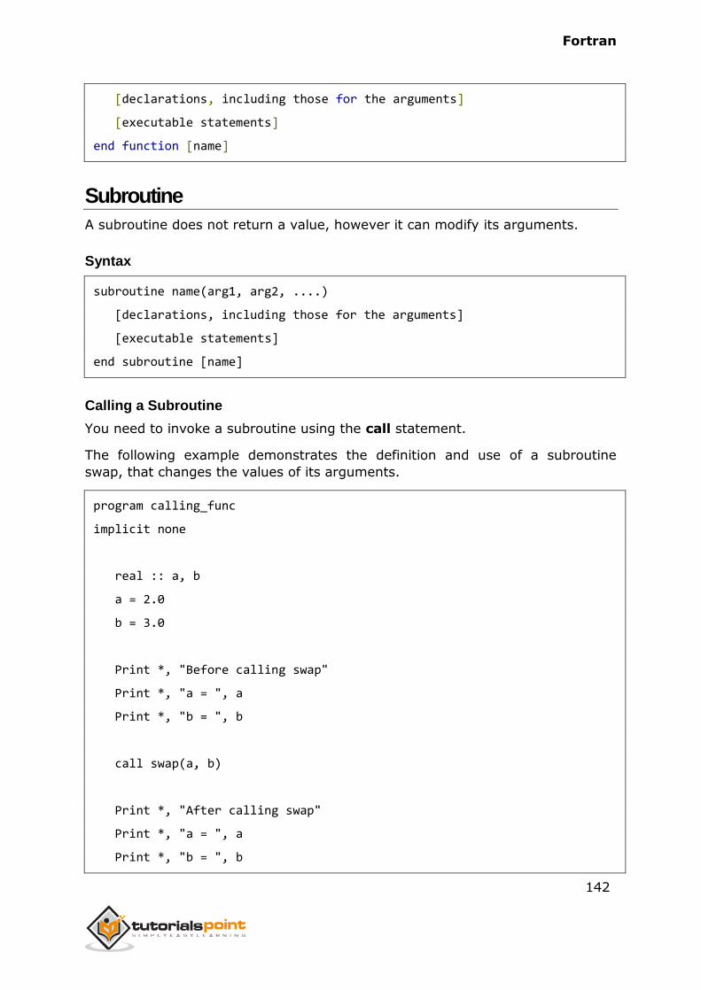
Fortran
142
[declarations, including those for the arguments]
[executable statements]
end function [name]
Subroutine
A subroutine does not return a value, however it can modify its arguments.
Syntax
subroutine name(arg1, arg2, ....)
[declarations, including those for the arguments]
[executable statements]
end subroutine [name]
Calling a Subroutine
You need to invoke a subroutine using the call statement.
The following example demonstrates the definition and use of a subroutine
swap, that changes the values of its arguments.
program calling_func
implicit none
real :: a, b
a = 2.0
b = 3.0
Print *, "Before calling swap"
Print *, "a = ", a
Print *, "b = ", b
call swap(a, b)
Print *, "After calling swap"
Print *, "a = ", a
Print *, "b = ", b
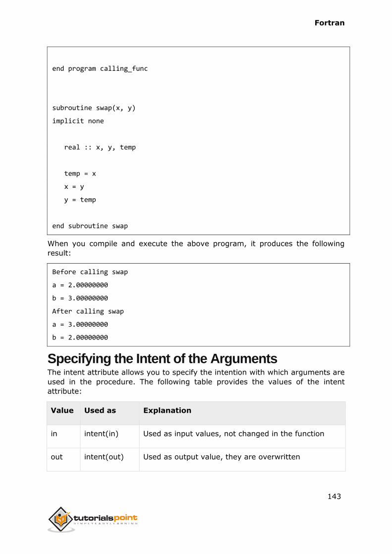
Fortran
143
end program calling_func
subroutine swap(x, y)
implicit none
real :: x, y, temp
temp = x
x = y
y = temp
end subroutine swap
When you compile and execute the above program, it produces the following
result:
Before calling swap
a = 2.00000000
b = 3.00000000
After calling swap
a = 3.00000000
b = 2.00000000
Specifying the Intent of the Arguments The intent attribute allows you to specify the intention with which arguments are
used in the procedure. The following table provides the values of the intent
attribute:
Value Used as Explanation
in intent(in) Used as input values, not changed in the function
out intent(out) Used as output value, they are overwritten
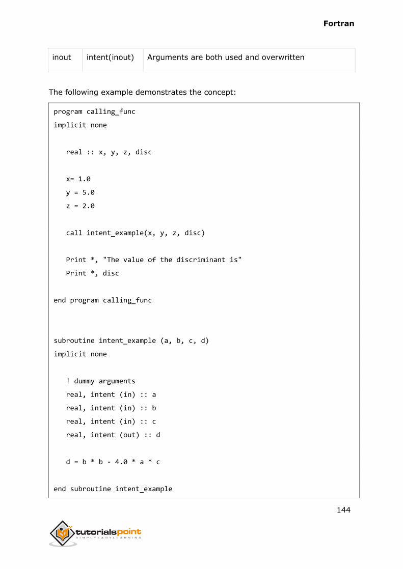
Fortran
144
inout intent(inout) Arguments are both used and overwritten
The following example demonstrates the concept:
program calling_func
implicit none
real :: x, y, z, disc
x= 1.0
y = 5.0
z = 2.0
call intent_example(x, y, z, disc)
Print *, "The value of the discriminant is"
Print *, disc
end program calling_func
subroutine intent_example (a, b, c, d)
implicit none
! dummy arguments
real, intent (in) :: a
real, intent (in) :: b
real, intent (in) :: c
real, intent (out) :: d
d = b * b - 4.0 * a * c
end subroutine intent_example
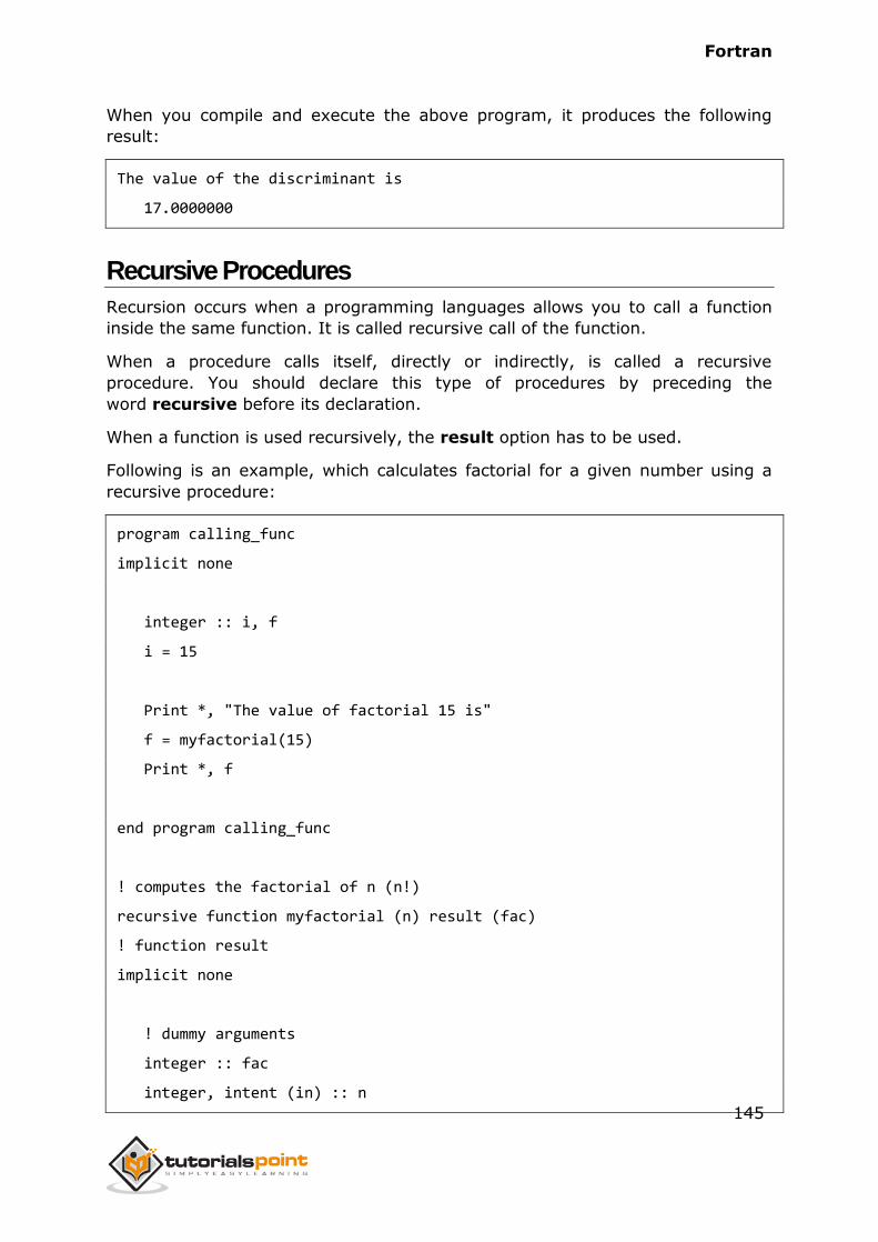
Fortran
145
When you compile and execute the above program, it produces the following
result:
The value of the discriminant is
17.0000000
Recursive Procedures
Recursion occurs when a programming languages allows you to call a function
inside the same function. It is called recursive call of the function.
When a procedure calls itself, directly or indirectly, is called a recursive
procedure. You should declare this type of procedures by preceding the
word recursive before its declaration.
When a function is used recursively, the result option has to be used.
Following is an example, which calculates factorial for a given number using a
recursive procedure:
program calling_func
implicit none
integer :: i, f
i = 15
Print *, "The value of factorial 15 is"
f = myfactorial(15)
Print *, f
end program calling_func
! computes the factorial of n (n!)
recursive function myfactorial (n) result (fac)
! function result
implicit none
! dummy arguments
integer :: fac
integer, intent (in) :: n
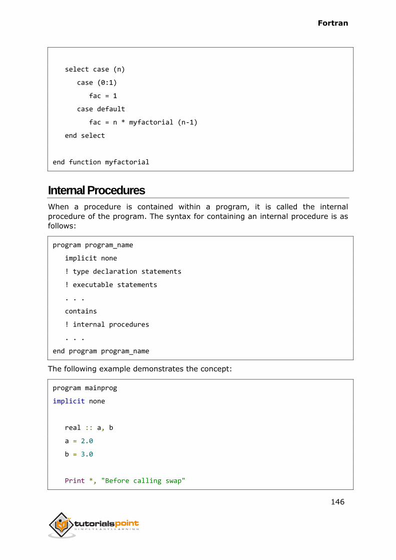
Fortran
146
select case (n)
case (0:1)
fac = 1
case default
fac = n * myfactorial (n-1)
end select
end function myfactorial
Internal Procedures
When a procedure is contained within a program, it is called the internal
procedure of the program. The syntax for containing an internal procedure is as
follows:
program program_name
implicit none
! type declaration statements
! executable statements
. . .
contains
! internal procedures
. . .
end program program_name
The following example demonstrates the concept:
program mainprog
implicit none
real :: a, b
a = 2.0
b = 3.0
Print *, "Before calling swap"

Fortran
147
Print *, "a = ", a
Print *, "b = ", b
call swap(a, b)
Print *, "After calling swap"
Print *, "a = ", a
Print *, "b = ", b
contains
subroutine swap(x, y)
real :: x, y, temp
temp = x
x = y
y = temp
end subroutine swap
end program mainprog
When you compile and execute the above program, it produces the following
result:
Before calling swap
a = 2.00000000
b = 3.00000000
After calling swap
a = 3.00000000
b = 2.00000000
Fortran
148
A module is like a package where you can keep your functions and subroutines,
in case you are writing a very big program, or your functions or subroutines can
be used in more than one program.
Modules provide you a way of splitting your programs between multiple files.
Modules are used for:
Packaging subprograms, data and interface blocks.
Defining global data that can be used by more than one routine.
Declaring variables that can be made available within any routines you
choose.
Importing a module entirely, for use, into another program or subroutine.
Syntax of a Module
A module consists of two parts:
a specification part for statements declaration
a contains part for subroutine and function definitions
The general form of a module is:
module name
[statement declarations]
[contains [subroutine and function definitions] ]
end module [name]
Using a Module into your Program
You can incorporate a module in a program or subroutine by the use statement:
use name
Please note that
You can add as many modules as needed, each will be in separate files
and compiled separately.
A module can be used in various different programs.
20. MODULES
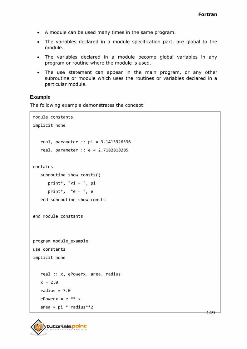
Fortran
149
A module can be used many times in the same program.
The variables declared in a module specification part, are global to the
module.
The variables declared in a module become global variables in any
program or routine where the module is used.
The use statement can appear in the main program, or any other
subroutine or module which uses the routines or variables declared in a
particular module.
Example
The following example demonstrates the concept:
module constants
implicit none
real, parameter :: pi = 3.1415926536
real, parameter :: e = 2.7182818285
contains
subroutine show_consts()
print*, "Pi = ", pi
print*, "e = ", e
end subroutine show_consts
end module constants
program module_example
use constants
implicit none
real :: x, ePowerx, area, radius
x = 2.0
radius = 7.0
ePowerx = e ** x
area = pi * radius**2
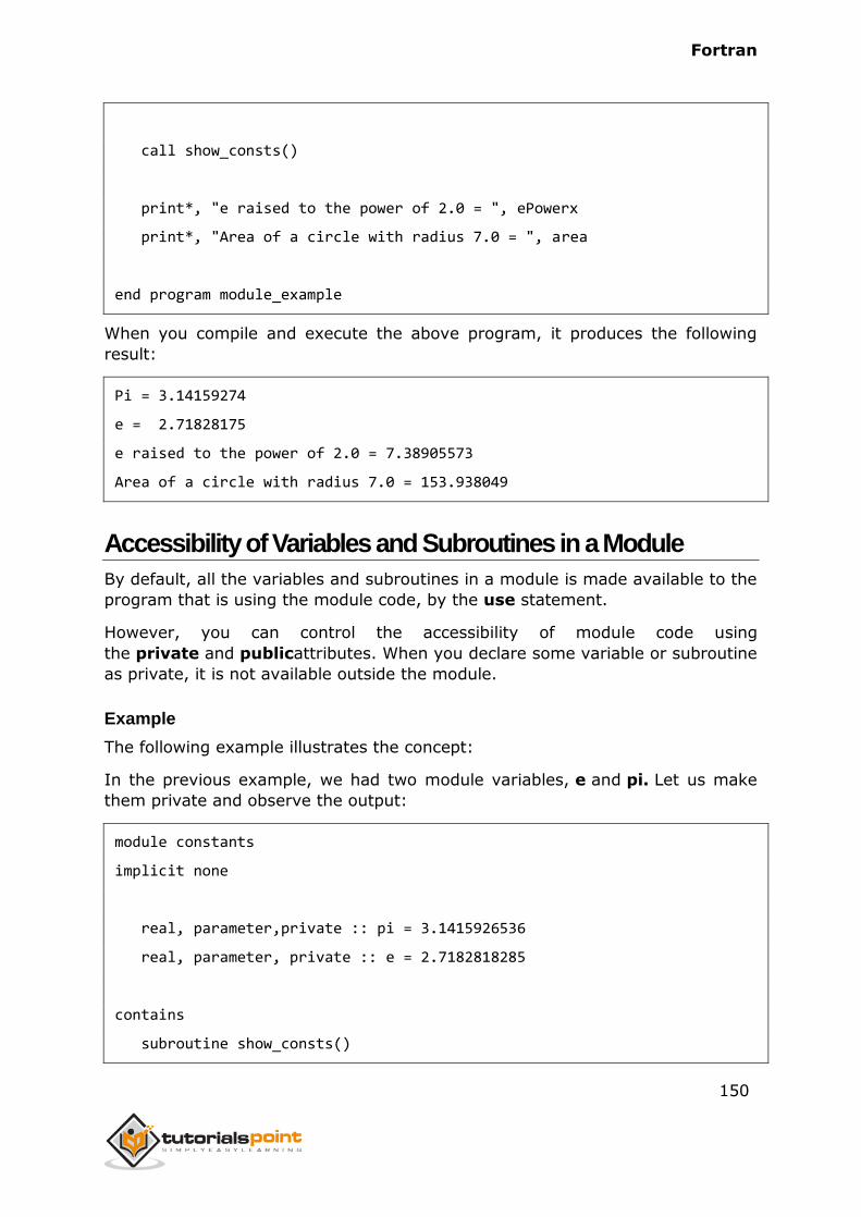
Fortran
150
call show_consts()
print*, "e raised to the power of 2.0 = ", ePowerx
print*, "Area of a circle with radius 7.0 = ", area
end program module_example
When you compile and execute the above program, it produces the following
result:
Pi = 3.14159274
e = 2.71828175
e raised to the power of 2.0 = 7.38905573
Area of a circle with radius 7.0 = 153.938049
Accessibility of Variables and Subroutines in a Module
By default, all the variables and subroutines in a module is made available to the
program that is using the module code, by the use statement.
However, you can control the accessibility of module code using
the private and publicattributes. When you declare some variable or subroutine
as private, it is not available outside the module.
Example
The following example illustrates the concept:
In the previous example, we had two module variables, e and pi. Let us make
them private and observe the output:
module constants
implicit none
real, parameter,private :: pi = 3.1415926536
real, parameter, private :: e = 2.7182818285
contains
subroutine show_consts()
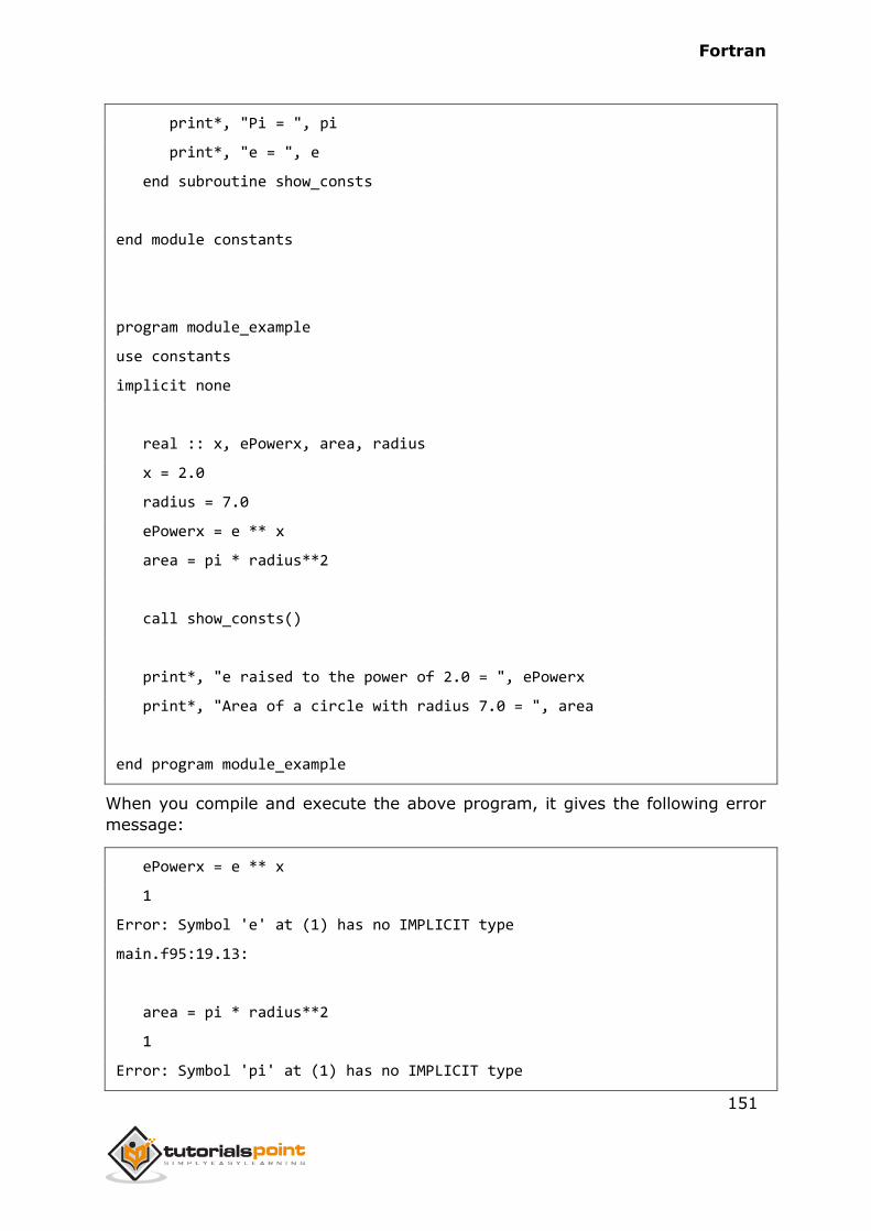
Fortran
151
print*, "Pi = ", pi
print*, "e = ", e
end subroutine show_consts
end module constants
program module_example
use constants
implicit none
real :: x, ePowerx, area, radius
x = 2.0
radius = 7.0
ePowerx = e ** x
area = pi * radius**2
call show_consts()
print*, "e raised to the power of 2.0 = ", ePowerx
print*, "Area of a circle with radius 7.0 = ", area
end program module_example
When you compile and execute the above program, it gives the following error
message:
ePowerx = e ** x
1
Error: Symbol 'e' at (1) has no IMPLICIT type
main.f95:19.13:
area = pi * radius**2
1
Error: Symbol 'pi' at (1) has no IMPLICIT type
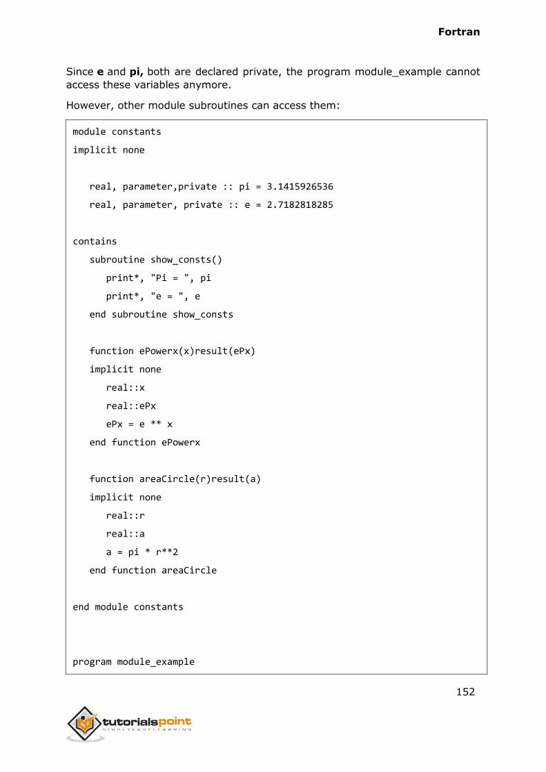
Fortran
152
Since e and pi, both are declared private, the program module_example cannot
access these variables anymore.
However, other module subroutines can access them:
module constants
implicit none
real, parameter,private :: pi = 3.1415926536
real, parameter, private :: e = 2.7182818285
contains
subroutine show_consts()
print*, "Pi = ", pi
print*, "e = ", e
end subroutine show_consts
function ePowerx(x)result(ePx)
implicit none
real::x
real::ePx
ePx = e ** x
end function ePowerx
function areaCircle(r)result(a)
implicit none
real::r
real::a
a = pi * r**2
end function areaCircle
end module constants
program module_example
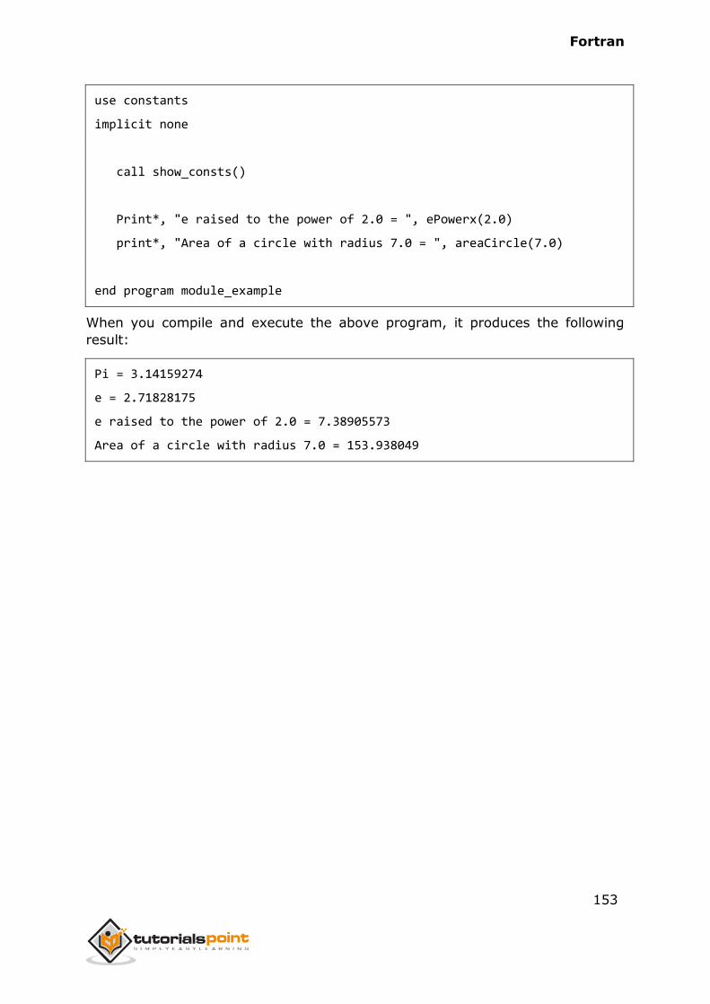
Fortran
153
use constants
implicit none
call show_consts()
Print*, "e raised to the power of 2.0 = ", ePowerx(2.0)
print*, "Area of a circle with radius 7.0 = ", areaCircle(7.0)
end program module_example
When you compile and execute the above program, it produces the following
result:
Pi = 3.14159274
e = 2.71828175
e raised to the power of 2.0 = 7.38905573
Area of a circle with radius 7.0 = 153.938049
Fortran
154
Intrinsic functions are some common and important functions that are provided
as a part of the Fortran language. We have already discussed some of these
functions in the Arrays, Characters and String chapters.
Intrinsic functions can be categorised as:
Numeric Functions
Mathematical Functions
Numeric Inquiry Functions
Floating-Point Manipulation Functions
Bit Manipulation Functions
Character Functions
Kind Functions
Logical Functions
Array Functions.
We have discussed the array functions in the Arrays chapter. In the following
section we provide brief descriptions of all these functions from other categories.
In the function name column,
A represents any type of numeric variable
R represents a real or integer variable
X and Y represent real variables
Z represents complex variable
W represents real or complex variable
Numeric Functions
Function Description
ABS (A) It returns the absolute value of A
AIMAG (Z) It returns the imaginary part of a complex number
21. INTRINSIC FUNCTIONS
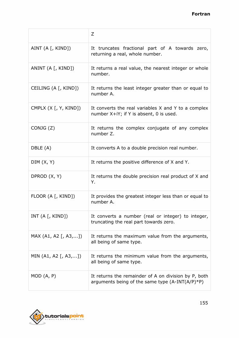
Fortran
155
Z
AINT (A [, KIND]) It truncates fractional part of A towards zero,
returning a real, whole number.
ANINT (A [, KIND]) It returns a real value, the nearest integer or whole
number.
CEILING (A [, KIND]) It returns the least integer greater than or equal to
number A.
CMPLX (X [, Y, KIND]) It converts the real variables X and Y to a complex
number X+iY; if Y is absent, 0 is used.
CONJG (Z) It returns the complex conjugate of any complex
number Z.
DBLE (A) It converts A to a double precision real number.
DIM (X, Y) It returns the positive difference of X and Y.
DPROD (X, Y) It returns the double precision real product of X and
Y.
FLOOR (A [, KIND]) It provides the greatest integer less than or equal to
number A.
INT (A [, KIND]) It converts a number (real or integer) to integer,
truncating the real part towards zero.
MAX (A1, A2 [, A3,...]) It returns the maximum value from the arguments,
all being of same type.
MIN (A1, A2 [, A3,...]) It returns the minimum value from the arguments,
all being of same type.
MOD (A, P) It returns the remainder of A on division by P, both
arguments being of the same type (A-INT(A/P)*P)
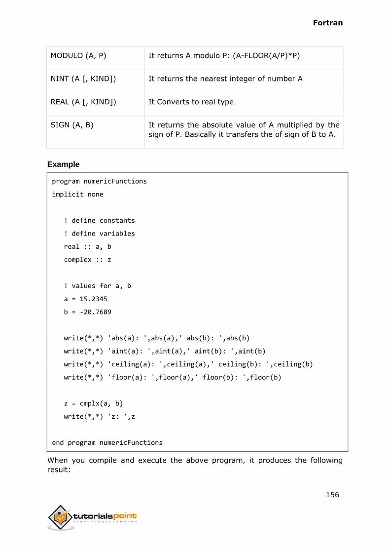
Fortran
156
MODULO (A, P) It returns A modulo P: (A-FLOOR(A/P)*P)
NINT (A [, KIND]) It returns the nearest integer of number A
REAL (A [, KIND]) It Converts to real type
SIGN (A, B) It returns the absolute value of A multiplied by the
sign of P. Basically it transfers the of sign of B to A.
Example
program numericFunctions
implicit none
! define constants
! define variables
real :: a, b
complex :: z
! values for a, b
a = 15.2345
b = -20.7689
write(*,*) 'abs(a): ',abs(a),' abs(b): ',abs(b)
write(*,*) 'aint(a): ',aint(a),' aint(b): ',aint(b)
write(*,*) 'ceiling(a): ',ceiling(a),' ceiling(b): ',ceiling(b)
write(*,*) 'floor(a): ',floor(a),' floor(b): ',floor(b)
z = cmplx(a, b)
write(*,*) 'z: ',z
end program numericFunctions
When you compile and execute the above program, it produces the following
result:
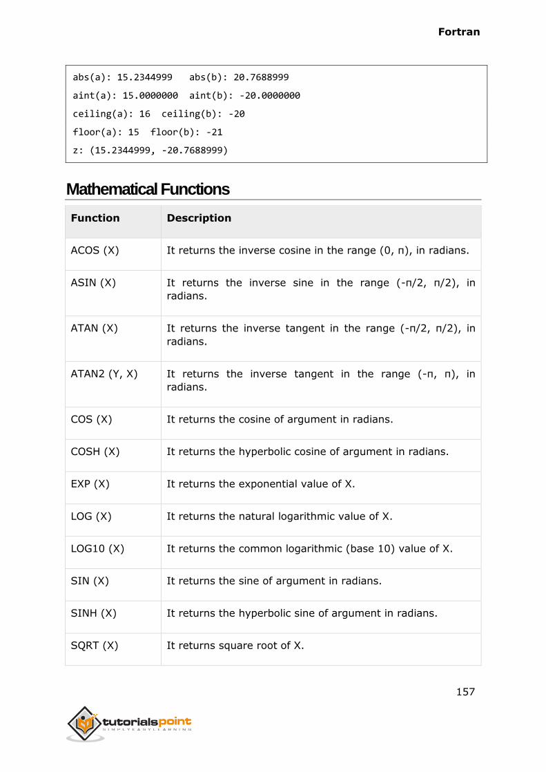
Fortran
157
abs(a): 15.2344999 abs(b): 20.7688999
aint(a): 15.0000000 aint(b): -20.0000000
ceiling(a): 16 ceiling(b): -20
floor(a): 15 floor(b): -21
z: (15.2344999, -20.7688999)
Mathematical Functions
Function Description
ACOS (X) It returns the inverse cosine in the range (0, π), in radians.
ASIN (X) It returns the inverse sine in the range (-π/2, π/2), in
radians.
ATAN (X) It returns the inverse tangent in the range (-π/2, π/2), in
radians.
ATAN2 (Y, X) It returns the inverse tangent in the range (-π, π), in
radians.
COS (X) It returns the cosine of argument in radians.
COSH (X) It returns the hyperbolic cosine of argument in radians.
EXP (X) It returns the exponential value of X.
LOG (X) It returns the natural logarithmic value of X.
LOG10 (X) It returns the common logarithmic (base 10) value of X.
SIN (X) It returns the sine of argument in radians.
SINH (X) It returns the hyperbolic sine of argument in radians.
SQRT (X) It returns square root of X.
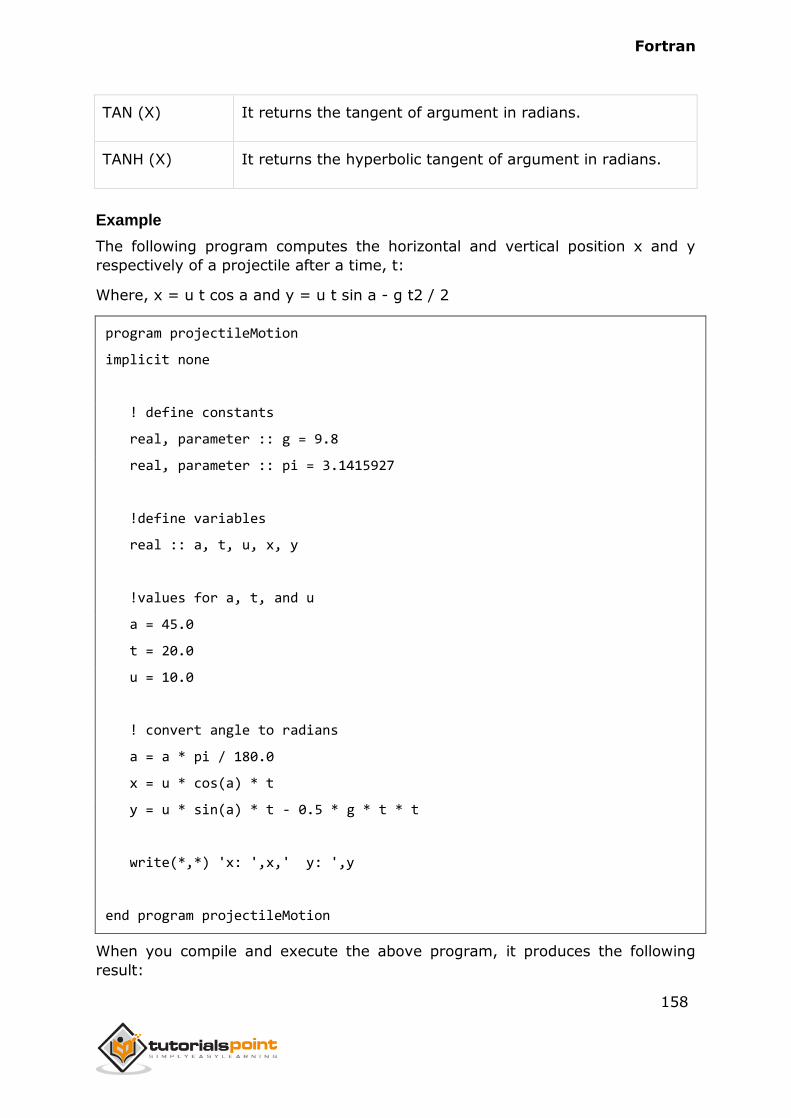
Fortran
158
TAN (X) It returns the tangent of argument in radians.
TANH (X) It returns the hyperbolic tangent of argument in radians.
Example
The following program computes the horizontal and vertical position x and y
respectively of a projectile after a time, t:
Where, x = u t cos a and y = u t sin a - g t2 / 2
program projectileMotion
implicit none
! define constants
real, parameter :: g = 9.8
real, parameter :: pi = 3.1415927
!define variables
real :: a, t, u, x, y
!values for a, t, and u
a = 45.0
t = 20.0
u = 10.0
! convert angle to radians
a = a * pi / 180.0
x = u * cos(a) * t
y = u * sin(a) * t - 0.5 * g * t * t
write(*,*) 'x: ',x,' y: ',y
end program projectileMotion
When you compile and execute the above program, it produces the following
result:
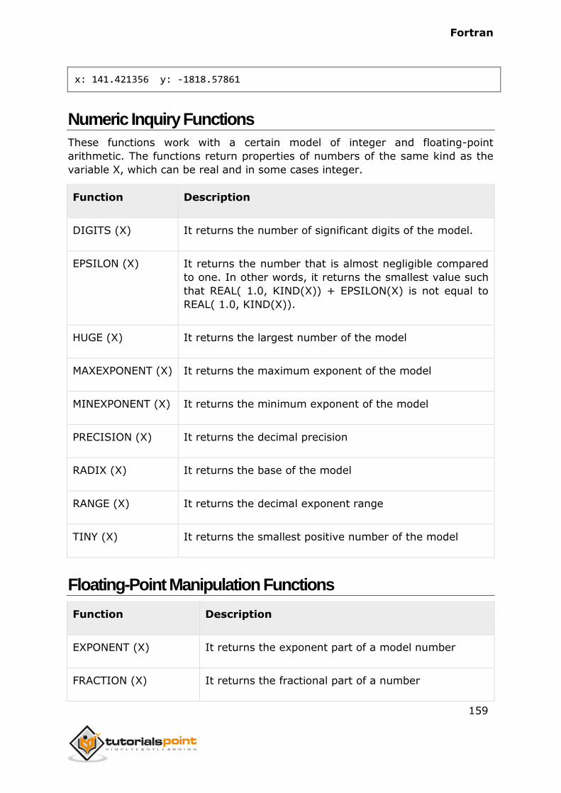
Fortran
159
x: 141.421356 y: -1818.57861
Numeric Inquiry Functions
These functions work with a certain model of integer and floating-point
arithmetic. The functions return properties of numbers of the same kind as the
variable X, which can be real and in some cases integer.
Function Description
DIGITS (X) It returns the number of significant digits of the model.
EPSILON (X) It returns the number that is almost negligible compared
to one. In other words, it returns the smallest value such
that REAL( 1.0, KIND(X)) + EPSILON(X) is not equal to
REAL( 1.0, KIND(X)).
HUGE (X) It returns the largest number of the model
MAXEXPONENT (X) It returns the maximum exponent of the model
MINEXPONENT (X) It returns the minimum exponent of the model
PRECISION (X) It returns the decimal precision
RADIX (X) It returns the base of the model
RANGE (X) It returns the decimal exponent range
TINY (X) It returns the smallest positive number of the model
Floating-Point Manipulation Functions
Function Description
EXPONENT (X) It returns the exponent part of a model number
FRACTION (X) It returns the fractional part of a number
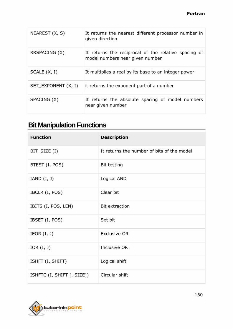
Fortran
160
NEAREST (X, S) It returns the nearest different processor number in
given direction
RRSPACING (X) It returns the reciprocal of the relative spacing of
model numbers near given number
SCALE (X, I) It multiplies a real by its base to an integer power
SET_EXPONENT (X, I) it returns the exponent part of a number
SPACING (X) It returns the absolute spacing of model numbers
near given number
Bit Manipulation Functions
Function Description
BIT_SIZE (I) It returns the number of bits of the model
BTEST (I, POS) Bit testing
IAND (I, J) Logical AND
IBCLR (I, POS) Clear bit
IBITS (I, POS, LEN) Bit extraction
IBSET (I, POS) Set bit
IEOR (I, J) Exclusive OR
IOR (I, J) Inclusive OR
ISHFT (I, SHIFT) Logical shift
ISHFTC (I, SHIFT [, SIZE]) Circular shift
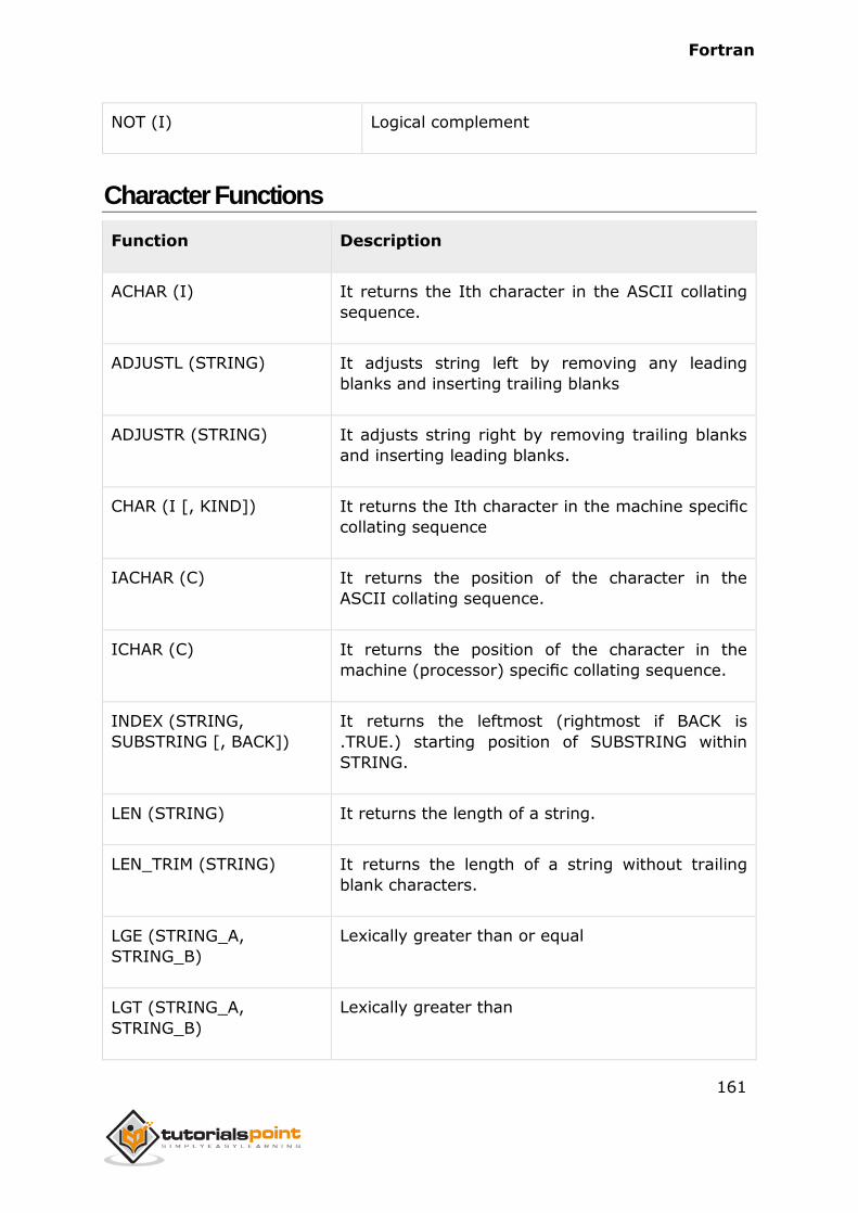
Fortran
161
NOT (I) Logical complement
Character Functions
Function Description
ACHAR (I) It returns the Ith character in the ASCII collating
sequence.
ADJUSTL (STRING) It adjusts string left by removing any leading
blanks and inserting trailing blanks
ADJUSTR (STRING) It adjusts string right by removing trailing blanks
and inserting leading blanks.
CHAR (I [, KIND]) It returns the Ith character in the machine specific
collating sequence
IACHAR (C) It returns the position of the character in the
ASCII collating sequence.
ICHAR (C) It returns the position of the character in the
machine (processor) specific collating sequence.
INDEX (STRING,
SUBSTRING [, BACK])
It returns the leftmost (rightmost if BACK is
.TRUE.) starting position of SUBSTRING within
STRING.
LEN (STRING) It returns the length of a string.
LEN_TRIM (STRING) It returns the length of a string without trailing
blank characters.
LGE (STRING_A,
STRING_B)
Lexically greater than or equal
LGT (STRING_A,
STRING_B)
Lexically greater than
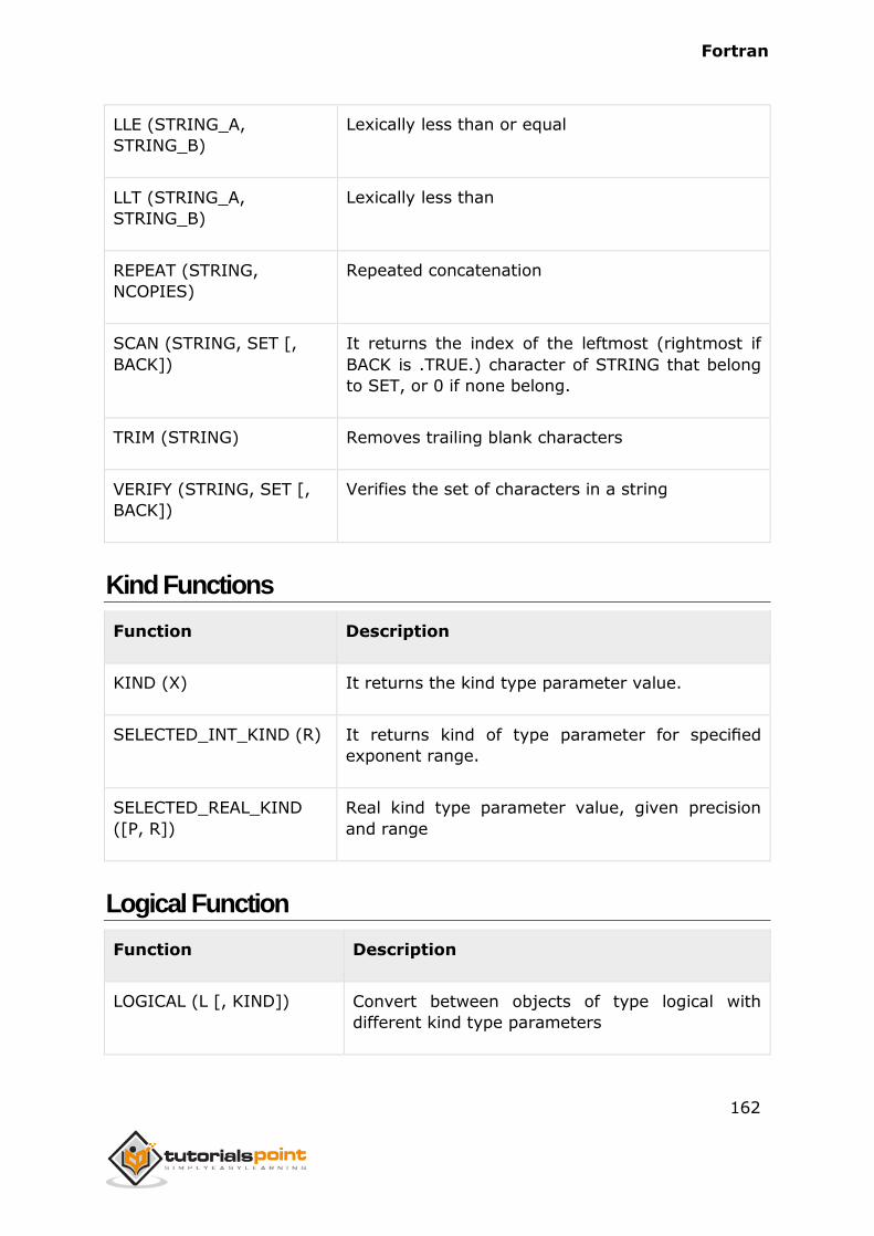
Fortran
162
LLE (STRING_A,
STRING_B)
Lexically less than or equal
LLT (STRING_A,
STRING_B)
Lexically less than
REPEAT (STRING,
NCOPIES)
Repeated concatenation
SCAN (STRING, SET [,
BACK])
It returns the index of the leftmost (rightmost if
BACK is .TRUE.) character of STRING that belong
to SET, or 0 if none belong.
TRIM (STRING) Removes trailing blank characters
VERIFY (STRING, SET [,
BACK])
Verifies the set of characters in a string
Kind Functions
Function Description
KIND (X) It returns the kind type parameter value.
SELECTED_INT_KIND (R) It returns kind of type parameter for specified
exponent range.
SELECTED_REAL_KIND
([P, R])
Real kind type parameter value, given precision
and range
Logical Function
Function Description
LOGICAL (L [, KIND]) Convert between objects of type logical with
different kind type parameters
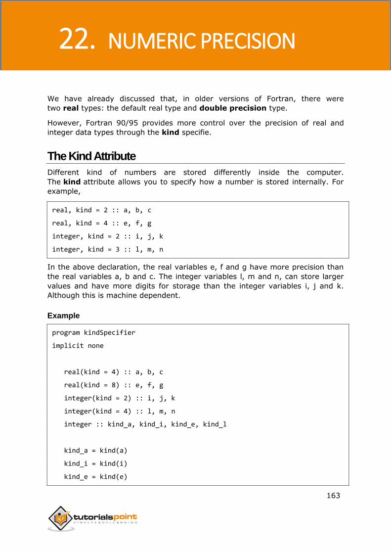
Fortran
163
We have already discussed that, in older versions of Fortran, there were
two real types: the default real type and double precision type.
However, Fortran 90/95 provides more control over the precision of real and
integer data types through the kind specifie.
The Kind Attribute
Different kind of numbers are stored differently inside the computer.
The kind attribute allows you to specify how a number is stored internally. For
example,
real, kind = 2 :: a, b, c
real, kind = 4 :: e, f, g
integer, kind = 2 :: i, j, k
integer, kind = 3 :: l, m, n
In the above declaration, the real variables e, f and g have more precision than
the real variables a, b and c. The integer variables l, m and n, can store larger
values and have more digits for storage than the integer variables i, j and k.
Although this is machine dependent.
Example
program kindSpecifier
implicit none
real(kind = 4) :: a, b, c
real(kind = 8) :: e, f, g
integer(kind = 2) :: i, j, k
integer(kind = 4) :: l, m, n
integer :: kind_a, kind_i, kind_e, kind_l
kind_a = kind(a)
kind_i = kind(i)
kind_e = kind(e)
22. NUMERIC PRECISION
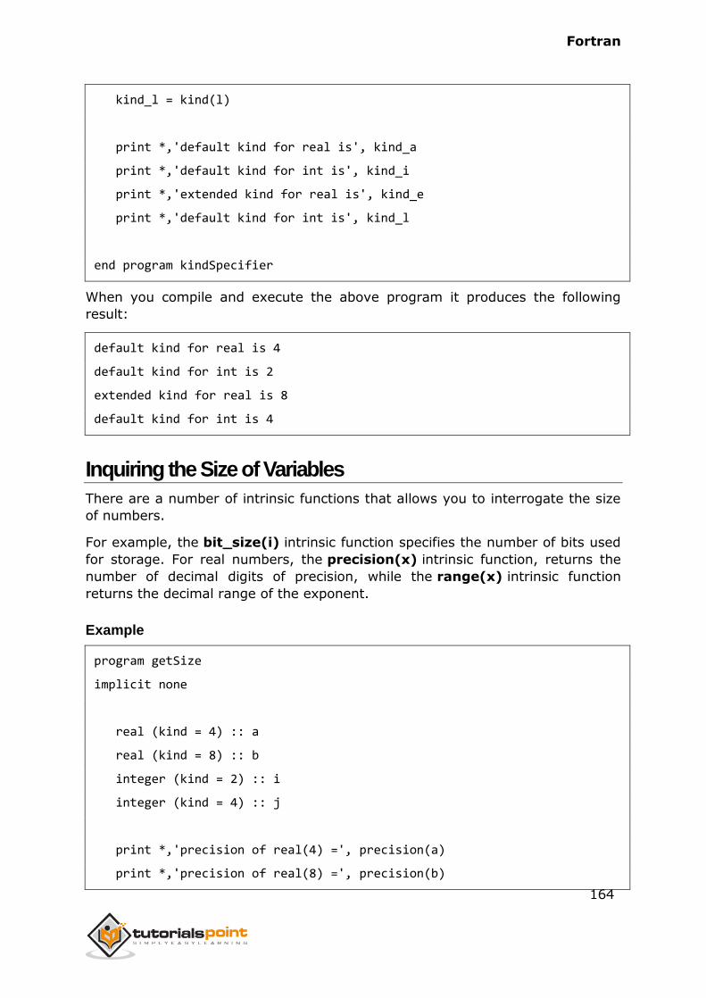
Fortran
164
kind_l = kind(l)
print *,'default kind for real is', kind_a
print *,'default kind for int is', kind_i
print *,'extended kind for real is', kind_e
print *,'default kind for int is', kind_l
end program kindSpecifier
When you compile and execute the above program it produces the following
result:
default kind for real is 4
default kind for int is 2
extended kind for real is 8
default kind for int is 4
Inquiring the Size of Variables
There are a number of intrinsic functions that allows you to interrogate the size
of numbers.
For example, the bit_size(i) intrinsic function specifies the number of bits used
for storage. For real numbers, the precision(x) intrinsic function, returns the
number of decimal digits of precision, while the range(x) intrinsic function
returns the decimal range of the exponent.
Example
program getSize
implicit none
real (kind = 4) :: a
real (kind = 8) :: b
integer (kind = 2) :: i
integer (kind = 4) :: j
print *,'precision of real(4) =', precision(a)
print *,'precision of real(8) =', precision(b)
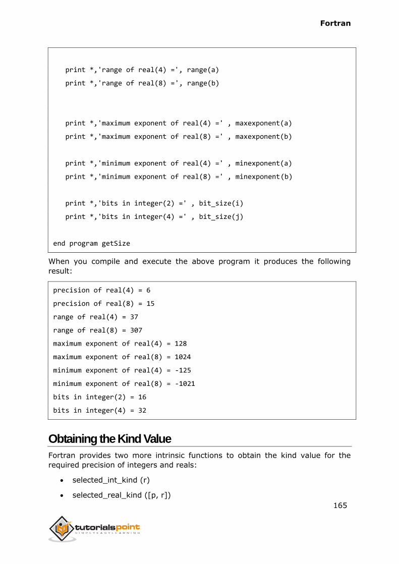
Fortran
165
print *,'range of real(4) =', range(a)
print *,'range of real(8) =', range(b)
print *,'maximum exponent of real(4) =' , maxexponent(a)
print *,'maximum exponent of real(8) =' , maxexponent(b)
print *,'minimum exponent of real(4) =' , minexponent(a)
print *,'minimum exponent of real(8) =' , minexponent(b)
print *,'bits in integer(2) =' , bit_size(i)
print *,'bits in integer(4) =' , bit_size(j)
end program getSize
When you compile and execute the above program it produces the following
result:
precision of real(4) = 6
precision of real(8) = 15
range of real(4) = 37
range of real(8) = 307
maximum exponent of real(4) = 128
maximum exponent of real(8) = 1024
minimum exponent of real(4) = -125
minimum exponent of real(8) = -1021
bits in integer(2) = 16
bits in integer(4) = 32
Obtaining the Kind Value
Fortran provides two more intrinsic functions to obtain the kind value for the
required precision of integers and reals:
selected_int_kind (r)
selected_real_kind ([p, r])
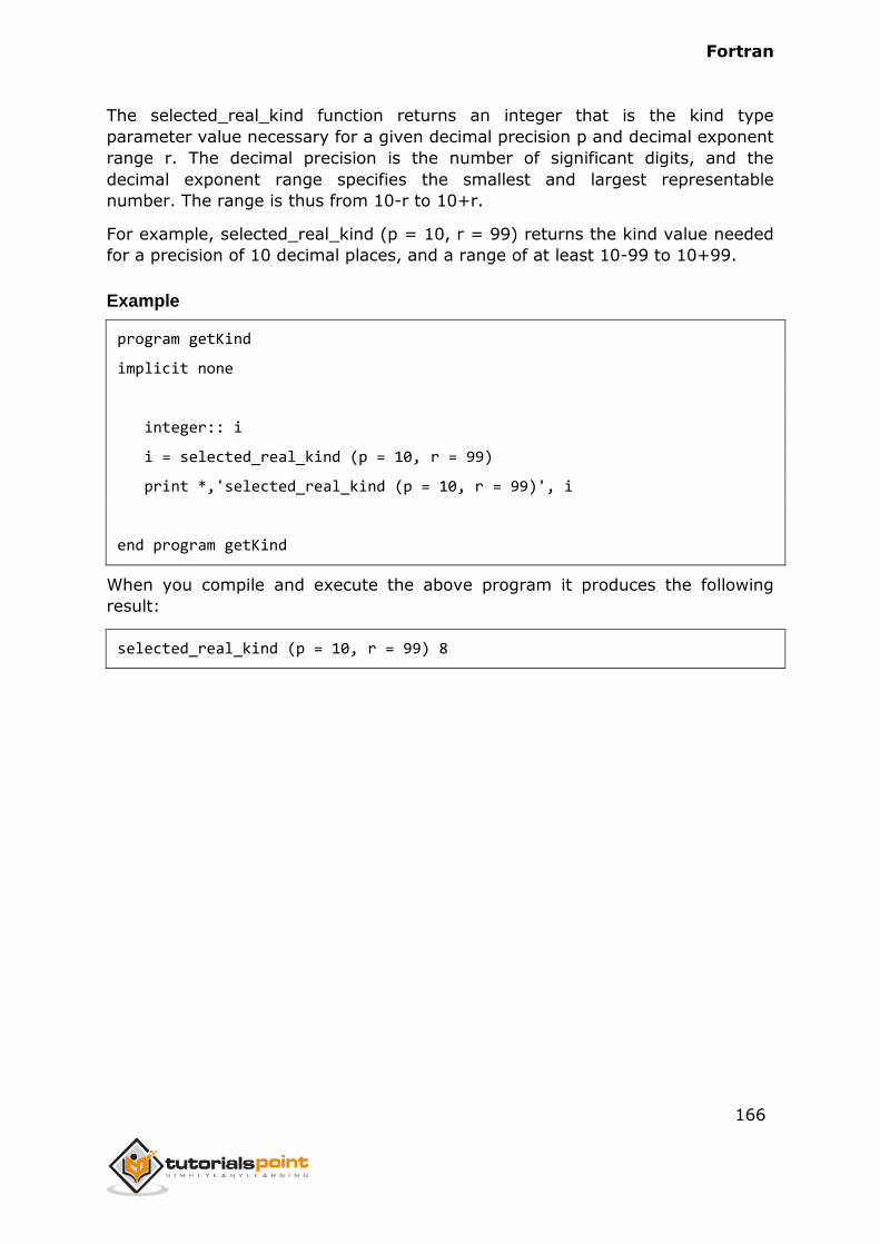
Fortran
166
The selected_real_kind function returns an integer that is the kind type
parameter value necessary for a given decimal precision p and decimal exponent
range r. The decimal precision is the number of significant digits, and the
decimal exponent range specifies the smallest and largest representable
number. The range is thus from 10-r to 10+r.
For example, selected_real_kind (p = 10, r = 99) returns the kind value needed
for a precision of 10 decimal places, and a range of at least 10-99 to 10+99.
Example
program getKind
implicit none
integer:: i
i = selected_real_kind (p = 10, r = 99)
print *,'selected_real_kind (p = 10, r = 99)', i
end program getKind
When you compile and execute the above program it produces the following
result:
selected_real_kind (p = 10, r = 99) 8
Fortran
167
There are various Fortran tools and libraries. Some are free and some are paid
services.
Following are some free libraries:
RANDLIB, random number and statistical distribution generators
BLAS
EISPACK
GAMS–NIST Guide to Available Math Software
Some statistical and other routines from NIST
LAPACK
LINPACK
MINPACK
MUDPACK
NCAR Mathematical Library
The Netlib collection of mathematical software, papers, and databases.
ODEPACK
ODERPACK, a set of routines for ranking and ordering.
Expokit for computing matrix exponentials
SLATEC
SPECFUN
STARPAC
StatLib statistical library
TOMS
Sorting and merging strings
The following libraries are not free:
The NAG Fortran numerical library
The Visual Numerics IMSL library
Numerical Recipes
23. PROGRAM LIBRARIES
Fortran
168
Programming style is all about following some rules while developing programs.
These good practices impart values like readability, and unambiguity into your
program.
A good program should have the following characteristics:
Readability
Proper logical structure
Self-explanatory notes and comments
For example, if you make a comment like the following, it will not be of
much help:
! loop from 1 to 10
do i=1,10
However, if you are calculating binomial coefficient, and need this loop for
nCr then a comment like this will be helpful:
! loop to calculate nCr
do i=1,10
Indented code blocks to make various levels of code clear.
Self-checking codes to ensure there will be no numerical errors like
division by zero, square root of a negative real number or logarithm of a
negative real number.
Including codes that ensure variables do not take illegal or out of range
values, i.e., input validation.
Not putting checks where it would be unnecessary and slows down the
execution. For example:
real :: x
x = sin(y) + 1.0
if (x >= 0.0) then
z = sqrt(x)
end if
24. PROGRAMMING STYLE
Fortran
169
Clearly written code using appropriate algorithms.
Splitting the long expressions using the continuation marker ‘&’.
Making meaningful variable names.
Fortran
170
A debugger tool is used to search for errors in the programs.
A debugger program steps through the code and allows you to examine the
values in the variables and other data objects during execution of the program.
It loads the source code and you are supposed to run the program within the
debugger. Debuggers debug a program by:
Setting breakpoints,
Stepping through the source code,
Setting watch points.
Breakpoints specify where the program should stop, specifically after a critical
line of code. Program executions after the variables are checked at a breakpoint.
Debugger programs also check the source code line by line.
Watch points are the points where the values of some variables are needed to be
checked, particularly after a read or write operation.
The gdb Debugger
The gdb debugger, the GNU debugger comes with Linux operating system. For X
windows system, gdb comes with a graphical interface and the program is
named xxgdb.
Following table provides some commands in gdb:
Command Purpose
break Setting a breakpoint
run Starts execution
cont Continues execution
next Executes only the next line of source code, without stepping into
any function call
step Execute the next line of source code by stepping into a function in
25. DEBUGGING PROGRAM
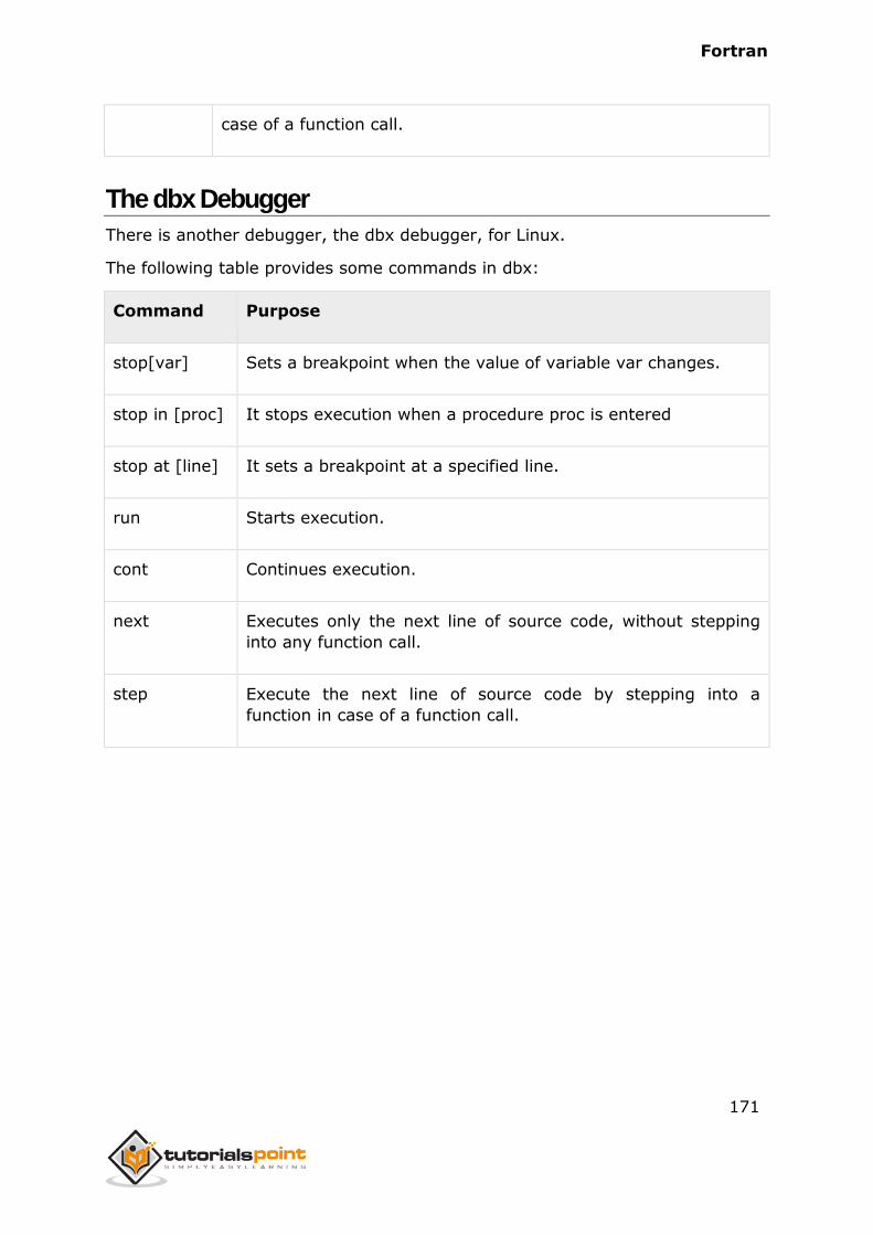
Fortran
171
case of a function call.
The dbx Debugger
There is another debugger, the dbx debugger, for Linux.
The following table provides some commands in dbx:
Command Purpose
stop[var] Sets a breakpoint when the value of variable var changes.
stop in [proc] It stops execution when a procedure proc is entered
stop at [line] It sets a breakpoint at a specified line.
run Starts execution.
cont Continues execution.
next Executes only the next line of source code, without stepping
into any function call.
step Execute the next line of source code by stepping into a
function in case of a function call.