forensics, elasticities and benford’s law: detecting...
TRANSCRIPT
Forensics, Elasticities and Benford’s Law:Detecting Tax Fraud in International Trade∗
Banu Demir†
Bilkent University and CEPR
Beata Javorcik‡
University of Oxford and CEPR
March 20, 2018
Abstract
By its very nature, tax evasion is difficult to detect as the parties involved havean incentive to conceal their activities. This paper offers a setting where doing so ispossible because of an exogenous shock to the tax rate. It contributes to the literatureby proposing two new methods of detecting evasion in the context of border taxes. Thefirst method is based on Benford’s law, while the second relies on comparing price andtrade cost elasticities of import demand. Both methods produce evidence consistentwith an increase in tax evasion after the shock. The paper further shows that evasioninduces a bias in the estimation of trade cost elasticity of import demand, leading tomiscalculation of gains from trade based on standard welfare formulations. Finally,welfare predictions are derived from a simple Armington trade model that accounts fortax evasion. JEL Codes: F10.
Keywords: Tax evasion, trade financing, border taxes, Benford’s law.
∗The authors would like to thank Andy Bernard, Maria Guadalupe, David Hummels, Oleg Itskhoki,Mazhar Waseem and Muhammed Ali Yildirim as well as seminar audiences at Warwick, King’s College, KocUniversity, Free University of Amsterdam, Aarhus, Copenhagen, Nottingham and the New Economic Schoolin Moscow for useful comments and discussions.†Department of Economics, Bilkent University, 06800 Ankara Turkey. [email protected]‡Department of Economics, University of Oxford, Manor Road Building Manor Road, Oxford OX1 3UQ,
1 Introduction
Wherever taxes are being collected, there is tax evasion. Yet, by its very nature, tax evasion
is difficult to detect as the parties involved have every incentive to conceal their lack of
compliance with the tax law. Tax evasion matters, as it may alter the distortionary costs of
raising tax revenue and affect the distributional consequences of a given tax policy. Resources
spent on tax evasion also represent a deadweight loss to the economy. Despite the great
importance of tax evasion to public policy choices, relatively little is known about the extent
of tax evasion and its responsiveness to tax rates. Finding answers to these questions is often
confounded by the lack of large and plausibly exogenous variation in tax rates.
This paper offers a setting where tax evasion can be detected because of a substantial
and exogenous shock to the tax rate. It contributes to the literature by proposing two new
methods of detecting tax evasion in the context of border taxes. The first method is based on
Benford’s law, which describes the distribution of first digits in economic or accounting data.
The second relies on comparing demand elasticities with respect to price and trade taxes.
Both methods are applied to an unexpected policy change in Turkey and uncover evidence
consistent with an increase in tax evasion after the Turkish authorities raised the tax rate
applied to external financing of imports. The increase in evasion matters, as taxes collected
by Turkish Customs amounted to USD 26.8 billion, or about 18% of total tax revenues in
Turkey, in 2011.
The paper further argues that incorporating a tax evasion channel is crucial to under-
standing the true impact of trade policy on economic activity. It demonstrates that evasion
induces a bias in the estimation of trade cost elasticity of import demand, leading to mis-
calculation of gains from trade based on standard welfare formulations. Finally, our study
shows theoretically the ambiguous welfare implications of tax evasion in the context of a
simple Armington trade model.
The unexpected policy shock exploited in this paper is the increase in the Resource Uti-
lization Support Fund (RUSF) tax which took place on 13 October 2011 in response to high
1
and persistent current account deficits. The tax rate was doubled, increasing from 3% to 6%
of the transaction value.1 The RUSF tax, in force since 1988, applies when credit is utilized
to finance the cost of imported goods. Whether or not an import transaction is subject to
the tax depends on the payment terms. Transactions financed through open account (OA),
acceptance credit (AC), and deferred payment letter of credit (DLC) are subject to the tax.2
Transactions financed in other ways (e.g., through cash in advance or a standard letter of
credit) are not. In other words, all imports for which the Turkish importer receives a trade
credit are subject to the tax.
Our empirical analysis identifies the effect of the policy change using both cross-sectional
and time-series variation. We use very detailed import data, including information on pay-
ment terms, to measure the exposure of a given product imported from a given source country
to the RUSF tax before the policy change. We then ask whether the post-shock evasion re-
sponse is systematically related to the pre-shock exposure to the tax. Put differently, our
identifying assumption is that import flows which are typically purchased on credit, and
thus are subject to the tax prior to the shock, will see a larger increase in evasion in the
post-shock period relative to imports that tended not to utilize external financing.
Before applying our new methods, we show that the “missing trade” approach, proposed
by Fisman and Wei (2004), produces evidence consistent with an increase in tax evasion after
the policy change. More specifically, we find that the increase in underreporting of imports
into Turkey (relative to exports figures reported by partner countries) after the policy change
is systematically related to exposure to the RUSF tax before the shock. The estimates imply
that import flows that came fully on credit (i.e., tax exposure equal to 100%) saw a 6% larger
increase in underreporting relative to flows with no exposure to the tax prior to the shock.
1Google Trends statistics, presented in Figure 1, show a large spike in the number of searches involving“KKDF” or “Kaynak Kullanımını Destekleme Fonu”, which is the Turkish name of the tax, in the week of9 October 2011. The number of searches was stable in the months preceding the policy change.
2Under the OA terms, foreign credit is utilized as the Turkish importer pays the exporter only afterreceiving the goods. Under the AC terms, domestic credit may be utilized: a bank sets up a credit facility onbehalf of the importer and provides financing for the purchase of goods. Finally, the DLC gives the importera grace period for payment: the importer receives goods by accepting the documents and agrees to pay thebank after a fixed period of time.
2
Our proposed detection method baseBenford’sd on Benford’s law, which describes the
distribution of leading digits in economic or accounting data and which is explained in detail
in Section 3.2, confirms this message. We use Turkish import data disaggregated by firm, 6
digit Harmonised System (HS) product, source country, month and payment method.3 For
each product-country-year cell, we calculate deviation from Benford’s law. Then we show
that cells with greater exposure to the RUSF tax prior to the shock have greater deviations
from Benford’s distribution after the policy change.
Next, we present a simple trade model, which predicts that the elasticity of imports with
respect to trade taxes is distorted in the presence of tax evasion. This prediction finds
support in the data. We estimate the import demand equation instrumenting for price
with a proxy for transport costs.4 The tax elasticity before the shock is found to be almost
identical to the estimated price elasticity, as predicted by the model in the absence of evasion.
After the shock, however, the estimated tax elasticity becomes substantially smaller, which
is consistent with an increase in tax evasion after the shock. This matters, because a biased
estimate of trade elasticity will lead to overestimation of welfare losses from the tax increase,
as calculated based on the widely used formula proposed by Arkolakis et al. (2012).
We close the paper with a discussion of how evasion affects welfare. We show theoretically
that tax evasion affects welfare through two channels. It lowers the actual tax rate and
affects the share of expenditure on domestic goods. Tax evasion unambiguously reinforces
gains from trade when tariff revenues are wasted because it lowers the domestic expenditure
share. However, it has an ambiguous effect when tariff revenues are being redistributed to
consumers.
The proposed method of detecting evasion based on Benford’s law may have practical
applications. A test showing a positive relationship between deviations from Benford’s law
3One may think of this data set as including transaction-level information aggregated to the monthlylevel.
4Our instrument is constructed as the sum of the distance between the province in which the Turkishimporter is located and Istanbul (the largest international port of Turkey) and the distance between Istanbuland the exporting country. The instrument captures variation in transport costs, which affects the quantitydemanded only through its effect on c.i.f. prices.
3

and the applicable tax/tariff rate would be quite suggestive of evasion taking place. Such
a test could be applied to import flows using a particular mode of transport, crossing a
particular checkpoint, or even being cleared by a particular customs officer. In contrast to
the “missing trade” method, it could be applied to high frequency data and to particular
types of flows, as partner country trade statistics are not required. Of course, as with any
statistical test, the possibility of type I and II errors should be kept in mind when interpreting
the results.
Our paper is related to several literatures. First, it contributes to the fast growing litera-
ture drawing attention to the abuse of public trust and regulations (Marion and Muehlegger
(2008), Casaburi and Troiano (2016), Artavanis et al. (2016), Fang and Gong (2017), and
Chen et al. (2017)). We extend this literature by showing evidence consistent with such
abuse taking place in the context of border taxes. Border taxes matter as they are collected
by every country in the world. And according to the World Customs Organization, taxes
collected by Customs, such as tariffs, consumption taxes, excise duties, etc., account for,
on average, 30 percent of government tax revenues. Not surprisingly, tax evasion is the top
issue on the policy agenda of Customs services around the world (Han (2014)).
Second, our work is related to the literature documenting tax evasion in international
trade using the “missing trade” approach (Fisman and Wei (2004); Fisman et al. (2008);
Javorcik and Narciso (2008); Mishra et al. (2008); Ferrantino et al. (2012); and Javorcik
and Narciso (2017)). Our paper contributes to this literature by proposing two alternative
methods of detecting tax evasion in international trade.
Third, our paper is related to the literature which studies the response of international
trade to changes in trade frictions (e.g. Feenstra (1995); Baier and Bergstrand (2001); Trefler
(2004); Yang (2008); Arkolakis et al. (2012); Felbermayr et al. (2015); Sequeira (2016); and
Goldberg and Pavcnik (2016)). While the existing literature overwhelmingly focuses on
tariffs and quotas, we focus on a non-tariff barrier to international trade: tax on import
financing. We contribute to this literature by providing another piece of evidence suggesting
4
that tax evasion affects gains from trade and the elasticity of trade with respect to tax rates.
Finally, our paper is related to an older literature on “directly-unproductive profit-
seeking” (DUP) activities such as tax evasion and lobbying. Bhagwati (1982) argues that
such activities limit the consumption possibilities available to consumers by diverting re-
sources from productive activities. However, Bhagwati and Srinivasan (1982) show that
DUP activities may improve welfare if they arise as a response to a distortionary govern-
ment policy. Our theoretical setting provides an example of this phenomenon. In particular,
we show that, provided that tax revenues are wasted, tax evasion reinforces gains from trade
by reducing the effective level of distortionary taxation.
The rest of the paper is structured as follows. Next section describes the institutional
context and data. Section 3 presents evidence of tax evasion based on the “missing trade”
approach and Benford’s law. Section 4 builds a simple Armington trade model with tax
evasion, which yields an empirical specification that we use to detect tax evasion. Finally,
section 5 provides the conclusions of our study.
2 Institutional Context and Data
2.1 Institutional Context
Turkey has become increasingly involved in international trade since the early 2000s: the
value of exports and imports increased five-fold between 1999 and 2013. While the country
trades with more than 200 countries, about 40% of its trade is with the European Union,
with whom Turkey has a customs union in manufacturing goods. Turkey’s considerably
low exports-to-imports ratio (about 65%) has been the main driver of its persistently large
current account deficit, which has remained above 5 percent of GDP since 2006 (except in
2009).
In response to this high and persistent current account deficit, on October 13, 2011,
5
Turkish authorities passed a law that increased the cost of import financing. The policy
increased the rate of the RUSF tax (discussed in the Introduction) from 3% to 6% of the
transaction value. An import transaction is subject to the RUSF tax if the importer is
provided with a credit facility. In particular, the following import payment terms are subject
to RUSF: open account (OA), acceptance credit (AC), and deferred payment letter of credit
(DLC). Under the OA terms, foreign credit is utilized as the Turkish importer pays the
exporter only after receiving the goods (usually 30 to 90 days). Under the AC terms,
domestic credit is utilized: a bank sets up a credit facility on behalf of the importer and
provides financing for the purchase of goods. Finally, the DLC gives the importer a grace
period for payment: the importer receives goods by accepting the documents and agrees
to pay the bank after a fixed period of time.5 The RUSF applies to ordinary imports as
processing imports have always been exempted from import duties and other taxation.
The Turkish law stipulates quite harsh penalties for noncompliance with the RUSF tax.
Although controversial, RUSF is considered an import duty and thus subject to the customs
laws and regulations, particularly with respect to penalties for noncompliance. Customs
law no. 4458 provides for extensive penalties, which includes the practice of “threefold of
import duties.” Accordingly, RUSF that is not collected is subject to penalties of three times
the underpayment. Considering that value added tax (VAT) is also assessed on the RUSF
payable upon importation, the penalty amount will also include an amount for three times
the underpaid VAT. Additionally, delay interest on the total amount will be assessed. As a
result, penalty amounts can quickly become significant (EY (2014), p. 32.)
Doubling of the tax rate from 3% to 6% of the transaction value can potentially wipe up
profit margins of some importers. They can respond to the shock in a number of ways. First,
they can reduce (or even stop) imports. Second, they can switch away from importing on
5The following payment methods are not subject to the RUSF: cash in advance (importer pre-pays andreceives the goods later); standard letter of credit (payment is guaranteed by the importer’s bank providedthat delivery conditions specified in the contract have been met); and documentary collection (which involvesbank intermediation without payment guarantee).
6
trade credit.6 However, moving away from trade credit is not trivial because it requires firms
to obtain credit elsewhere. Given the unexpected nature of the tax hike, not every importer
would be able to obtain credit on a short notice. Some importers may not have access to
credit at all. For others, the 6% tax rate on trade credit may still be more advantageous
than the cost of credit.7 The final possibility is evasion.
It is unlikely that importers evade by misreporting the financing terms of the transaction.
The Turkish Customs requires a proof of the financing terms in the form of official bank
documents and obtaining official bank documents for fictitious transactions is very difficult.
A more likely scenario is the following. The export and import declarations do not mention
specifics of what is being exported/imported, but only the number of the commercial invoice
that has these details. The evading importer needs to obtain two invoices with the same
number, with the same or different details about the products, but with different total
values. When the shipment leaves the exporting country, it is accompanied by the expensive
invoice, as exporters may wish to collect a VAT refund. But when the shipment enters
Turkey, the cheaper invoice is attached to the import declaration. This procedure works as
long as the customs authorities of the different countries do not exchange information. It is,
therefore, used a lot between countries whose governments are not on particularly friendly
terms. According to an employee of a trucking company located in an Eastern European
country, this procedure almost never fails.
2.2 Data
The main dataset used in our empirical analysis is the Trade Transactions Database (TTD),
a confidential dataset provided by the Turkish Statistics Institute (TUIK), which contains
detailed information on Turkish firms’ transactions with the rest of the world over the 2010-
6In the next subsection, we present evidence illustrating decline in firm-level imports purchased withtrade credit.
7Interest rates in Turkey are high. The average deposit interest rate in the third quarter of 2011 was8.4%.
7
2012 period. The data, collected by the Ministry of Customs and Trade of the Republic
of Turkey, are based on the customs declarations filled in every time an international trade
transaction takes place. TTD reports the quantity and the value of firm-level imports in
US dollars by product, classified according to the 6-digit Harmonised System (HS), source
country, date of the transaction (month and year), payment method (e.g. cash in advance,
open account, letter of credit, etc.) and trade regime (ordinary and processing).8 Import
values include cost, insurance and freight (c.i.f.). We restrict the sample to the trading
partners which are members of the World Trade Organization.
We aggregate monthly trade flows into annual data to cover 24‘months before and 12
months after the date of the policy change (October 2011). In particular, we construct three
12-month periods: t = {T−2, T−1, T}, where T−2 covers the October 2009-September 2010
period, T − 1 covers October 2010-September 2011, and T covers October 2011-September
2012.
We measure the RUSF tax exposure of product h from source country c imported at time
t as:
Exposurehct =
∑m∈{OA,AC,DLC}Mhcmt∑
mMhcmt
, (1)
where Mhcmt denotes the value of imports of product h from country c on payment method
m at time t. The numerator gives the sum of product-country-level imports on OA, AC,
and DLC terms at time t, which are subject to the tax, and the denominator is equal to
the value of total imports during the same period. A higher value of Exposurehct implies
a greater reliance on external financing and thus a greater exposure to the increase in the
RUSF tax rate.
Although, to the best of our knowledge, the RUSF tax rate increase was unexpected, in our
analysis we take a conservative approach and focus on exposure 24 months before the shock
8In the data, ordinary imports account for about 85% total imports.
8
(October 2009-September 2010), Exposurehc,T−2.9 In this way, we eliminate the possibility
that some importers have adjusted their behavior in anticipation of the tax increase, though,
as we argued earlier, the available evidence suggests that the policy change was unanticipated.
The tax increase mattered. As illustrated in Figure 2, the distribution of Exposurehc for
ordinary imports (in the upper panel) shifted to the left after the increase in the RUSF rate.
In particular, the average value of the share of imports with external financing decreased
from about 20% to 14% after the shock. As expected, the distribution of Exposurehc for
processing imports, which are exempt from any type of tax, remained unchanged after the
shock (see the lower panel).
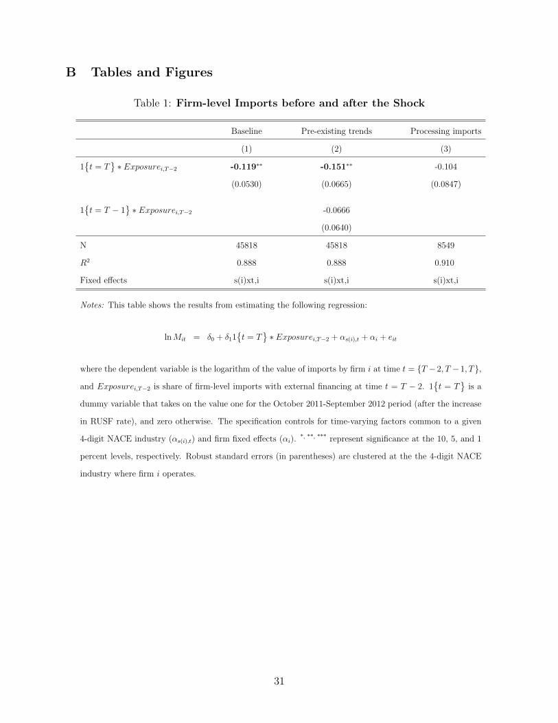
The tax increase also affected the magnitude of trade flows. A difference-in-differences
analysis (presented in Table 1) shows that imports of firms with a greater initial reliance
on external financing decreased in relative terms after the increase in the RUSF rate. The
estimated effect is economically significant: a one-standard-deviation increase in the share of
imports with external financing before the shock was associated with imports declining by
about 5% after the policy change. No such change is visible for processing imports purchased
on trade credit, as they are not subject to the tax.
3 Preliminary Evidence on Tax Evasion
3.1 “Missing trade” approach
To investigate the effect of the policy change on tax evasion, we first rely on the “missing
trade” approach developed by Fisman and Wei (2004). Focusing on Turkey’s imports of
product h from country c at time t, we construct a variable that captures the gap between
9The October 2009-September 2010 period overlaps with the Great Recession, which was characterizedby a major worldwide disruption of trade finance. However, the distribution of the share of Turkish importsutilizing external financing does not show a significant change during this period relative to the pre-crisisperiod.
9
the value of the flow reported by the source country c and the value reported by Turkey:
MissingTradehct = lnXchct − lnMTUR
hct ,
where lnXchct is logarithm of country c’s exports of product h to Turkey as reported by c, and
lnMTURhct is the logarithm of imports of h from c as reported by Turkey. As export figures are
reported on f.o.b. basis and import statistics include freight and insurance charges (i.e., they
are reported on c.i.f. basis), we expect MissingTrade to be negative. However, on average
the reported exports exceeded the imports by 1.4% in 2010 and 3.3% in 2011. Implementing
the “missing trade” approach to detecting evasion requires export data reported by Turkey’s
partner countries. We obtain annual trade data from United Nations COMTRADE database.
When we focus on flows that are reported by both Turkey and a partner country, we have
information on annual imports for 4,295 6-digit HS products from 98 partner countries over
the 2010-2012 period. The database also reports the weight of each flow, which we use to
construct unit values (value per kilogram).10
In the top panel of Figure 3, we plot local polynomial regressions of MissingTrade in
the year prior to the shock and after the shock as a function of Exposurehc,T−2. As evident
from the figure, MissingTrade increases with exposure to the tax. More interestingly, the
MissingTrade curve shifts up at all levels of Exposure in the post-shock period with the
upward shift being the largest for flows with the highest exposure to the tax.
The bottom panel plots local polynomial regressions of ∆ lnXchct and ∆ lnMTUR
hct as func-
tions of Exposurehc,T−2. As expected, regardless of the reporting partner, Turkish imports
decreased with the initial share of trade subject to the tax. More importantly, the wedge
between ∆ lnXchct and ∆ lnMTUR
hct is increasing with the initial exposure, which is consistent
with an increase in tax evasion after the hike in the RUSF tax rate in October 2011. To test
whether underreporting of imports after the policy change increases systematically with the
10Due to shipping lags, matching flows reported by the exporter and the importer at higher frequencieswould be problematic. Therefore, we use annual trade data in this exercise.
10
initial exposure to the tax, we estimate the following equation:
MissingTradehct = γ0 + γ11{t = T} ∗ Exposurehc,T−2 + αht + αct + αhc + εhct. (2)
The equation controls for unobservable heterogeneity at the product-country level with αhc
fixed effects as well as for time-varying product (αht) and country (αct) fixed effects. Note
that because Exposurehc,T−2 is time invariant, its impact will be captured by product-
country fixed effects. Our coefficient of interest is γ1 whose positive value would be consistent
with an increase in tax evasion after the hike in the RUSF tax rate in October 2011. The
results obtained from estimating equation (2) are presented in the first column in the upper
panel of Table 2. Our coefficient of interest γ1 is positive and statistically significant at the 5%
level. It implies that increasing Exposure from zero to one increases MissingTrade by about
6 percent after the RUSF hike. We also investigate the channels through which evasion may
take place; importers may underreport quantities and/or prices. The results presented in the
second and third columns suggest that evasion tends to take place through underreporting of
prices rather than quantities, though the coefficient in the quantity estimation is relatively
large, albeit statistically insignificant.11
In the lower panel of Table 2, we include 1{t = T − 1} ∗Exposurehc,T−2 as an additional
control to show that the baseline results reflect the effect of the policy change at t = T and
not just a pre-existing trend. This is indeed the case. Note that the results in column (2) do
not suggest absence of tax evasion prior to the RUSF rate increasing from 3% to 6%. They
only show that there was no increase in the extent of evasion in the year prior to the policy
change. As there was no border-tax-related policy change prior to the shock we consider,
there is no reason to expect changes in the extent of evasion at T − 1.12
11When interpreting these results one should keep in mind the imperfect measurement of prices, whichare defined as value per kg.
12The relationship between “Missing trade” and Exposurehc,T−2, which would be indicative of evasiontaking place already prior to 2012, is not visible in the table. It is because product-country (αhc) fixed effectsincluded in each specification capture the impact of Exposurehc,T−2, and hence this variable does not enterthe specification.
11
Table 3 reports two robustness checks. The upper panel explores whether the response
of “missing trade” to the initial tax exposure is non-linear. It is done by creating indicators
for bins based on quartiles of Exposurehc,T−2. The results are consistent with the patterns
illustrated in Figure 3. The gap between exports reported by partner countries and imports
recorded by Turkey increases little at the bottom quartile of Exposurehc,T−2 but increases
greatly for higher quartiles. The lower panel of the table shows the results from a falsification
test where we construct Exposureplacebo using processing imports which are exempt from
any type of tax. As expected, the coefficient of interest γ1 does not retain its statistical
significance in the placebo specification.
3.2 Benford’s law
Our first alternative approach to detecting evasion relies on Benford’s law. Benford’s law
describes the distribution of first (or leading) digits in economic or accounting data.13 The
law predicts that a given leading digit d will occur with the following probability:
P (First digit is d) = log10(1 + 1/d) (3)
The law naturally arises when data are generated by an exponential process or independent
processes are pooled together (see Figure 4 for the predicted distribution of leading digits
according to the law). Deviations from Benford’s distribution have been used to detect
reporting irregularities in macroeconomic data (Michalski and Stoltz (2013)) and in survey
data (Judge and Schechter (2009)).
We expect Benford’s law to hold in our data for the following reasons. First, “second-
generation” distributions, i.e., combinations of other distributions, such as, quantity×price
(as in our case) conform with Benford’s law (Hill (1995). Second, distributions where mean
is greater than median and skew is positive have also been shown to comply with Benford’s
13For instance, in the number 240790, digit 2 is the leading digit.
12
law (Durtschi et al. (2004)). Figure 5 demonstrates that the distribution of import values
in our data is positively skewed, with a mean greater than the median value.
Our hypothesis is that while Benford’s law should hold in import data, it will not hold if
the data have been manipulated for the purposes of tax evasion. It is because, as shown by
experimental research, people do a poor job of replicating known data-generating processes,
by for instance over-supplying modes or under-supplying long runs (Camerer (2003), pp.
134-138).14 Moreover, since Benford’s law is not widely known, it seems very unlikely that
those manipulating numbers would seek to preserve fit to the Benford distribution.
We start by performing a simple χ2 test to check whether our import data conform with
Benford’s law. We use the data obtained from TTD aggregated to the level of 6-digit product
and source country for the 12-month periods T and T−1. We consider ordinary trade only, as
processing trade is not subject to any border taxes. We construct the data by first grouping
transactions by treatment status, i.e. subject to RUSF or not, in each period and then
aggregating each sub-sample at the 6-digit HS and destination country level. Table 4 shows
that ordinary imports that are not subject to the RUSF tax conform with the law both at
t = T and t = T − 1. However, when we consider ordinary imports subject to the RUSF
tax, their distribution conforms with the law before the tax hike but not afterwards. This
finding is consistent with the message from the “missing trade” exercise, which suggests that
evasion in the aftermath of the policy change was rising with exposure to the tax.
Next, we use a difference-in-differences approach to test whether the distribution of Turk-
ish imports deviated significantly from Benford’s law after the policy change and whether
this deviation was systematically related to the initial exposure to the tax. To do so, we
follow Cho and Gaines (2007) and Judge and Schechter (2009) and use the following distance
14An example given by Hill (1999) (p. 27) illustrates this point nicely: “To demonstrate this [the difficultyof fabricating numerical data successfully] to beginning students of probability, I often ask them to do thefollowing homework assignment the first day. They are either to flip a coin 200 times and record the resultsor merely pretend to flip a coin and fake the results. The next day I amaze them by glancing at eachstudent’s list and correctly separating nearly all the true from the faked data. The fact in this case is thatin a truly random sequence of 200 tosses it is extremely likely that a run of six heads or six tails will occur(the exact probability is somewhat complicated to calculate), but the average person trying to fake such asequence will rarely include runs of that length.”
13
measure to capture deviations from Benford’s law:
D =9∑d=1
(fd − fd)2, (4)
where fd denotes the observed fraction of leading digit d in the data, and fd fraction predicted
by Benford’s law. For each product-country hc pair with at least 30 observations, we calculate
respective frequencies, fdhct to construct Dhct. The summary statistics are presented in Table
5. We estimate the following specification:
Dhct = θ0 + θ11{t = T} ∗ Exposurehc,T−2 + αht + αct + αhc + ehct, (5)
which controls for product-year, country-year and product-country fixed effects. We antici-
pate a positive estimate of θ1 which would be consistent with an increase in tax evasion after
the hike in the RUSF tax rate in October 2011.
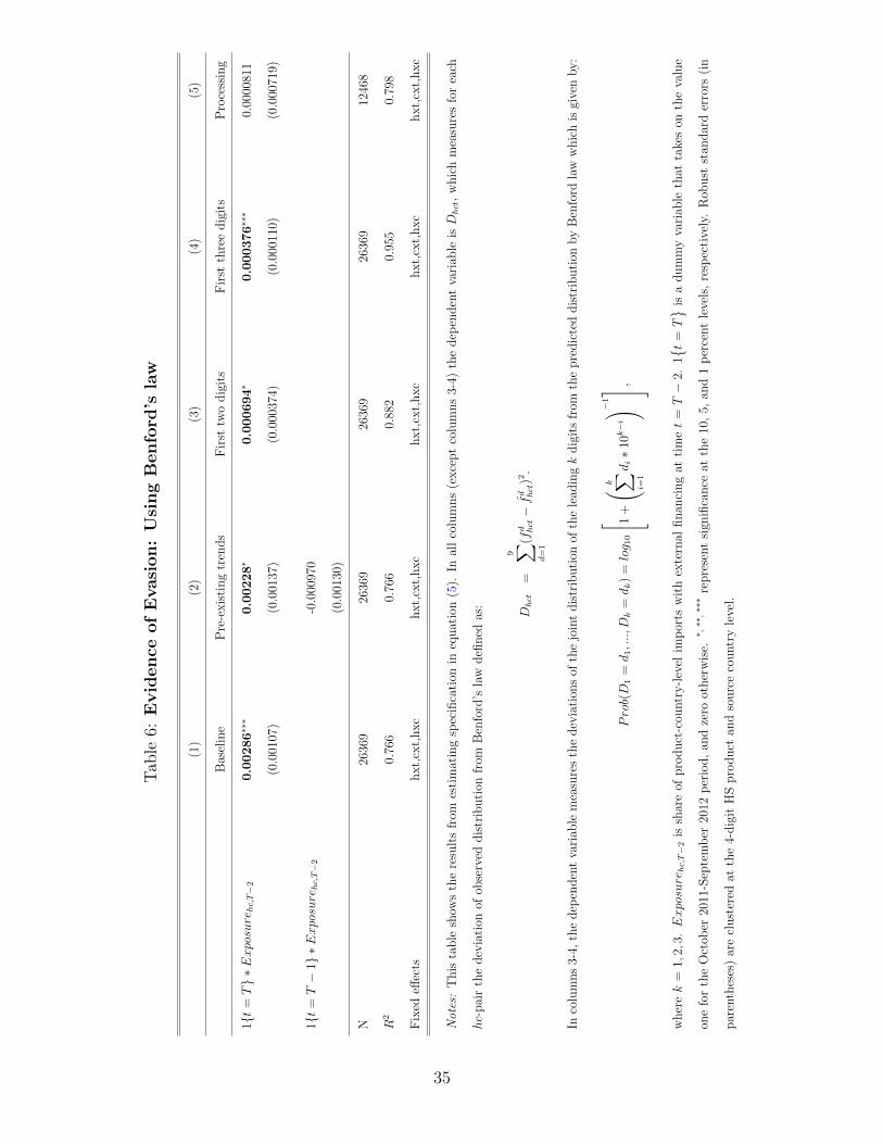
This alternative approach to detecting tax evasion yields results supporting our earlier
conclusions. The results in column 1 of Table 6 show that an increase in deviation from
Benford’s law after the shock is positively correlated with the initial exposure to the tax.
The estimates imply that going from no exposure to the tax to a full exposure (i.e., increase
from 0 to 1) increases the deviation from Benford’s Law by 17% relative to the mean value
of D at t = T − 1.15 In the second column of Table 6, we show that allowing for pre-existing
trends does not affect the estimate of our coefficient of interest.
In columns 3-4, we conduct a robustness test where we test the deviation of the joint
distribution of the leading two or three digits from their respective distributions predicted
15To put this figure into perspective consider a random sample with characteristics similar to an averageproduct-country cell in our sample before the shock, that is, a collection of numbers with D = 0.0172. Nowadd “faked” observations which do not follow Benford’s law. Instead, assume that a “faked” observationis equally likely to start with digit 1, 2, 3, etc. What is the fraction of “faked” observations required togenerate the estimated increase in D due to exposure going from 0 to 1? It is about 40%.
14
by Benford law:
Prob(D1 = d1, ..., Dk = dk) = log10
1 +
(k∑i=1
di ∗ 10k−i
)−1 ,
where k = 1, 2, 3; d1 ∈ {1, 2, ..., 9} and d2, d3 ∈ {0, 1, 2, ..., 9}. As in the baseline exercise,
we construct deviations of the observed distribution from the predicted distribution and re-
estimate equation (5). The results are in line with the baseline findings which point to an
increase in evasion after the increase in the RUSF rate in October 2011.
In the fifth column, we conduct a placebo exercise by focusing on processing trade which
is not subject to any border taxes and where we would not expect to see an increase in
deviation from Benford’s law after the policy change. The results confirm our priors. The
coefficient of interest is not statistically significant and its magnitude is very close to zero.
4 A Theoretical Approach to Detecting Tax Evasion
4.1 Setup
In this section, we propose an alternative approach to detecting tax evasion in international
trade transactions, which relies on comparing price and tax elasticity of demand for imports.
While the approach is not new in public economics (e.g. Marion and Muehlegger (2008)), it
has not been used to detect tax evasion in international trade.
Compared to a standard taxation model in public economics, our setting poses an impor-
tant challenge. Whether or not a transaction is subject to the RUSF tax is an endogenous
decision taken by an importer. The reason is that the tax applies only when external fi-
nancing is used when importing. Therefore, the importer decides whether to evade taxes,
conditional on using external financing.
Consider a simple Armington model of international trade with n+ 1 countries, indexed
15

by c. We refer to Turkey as the home country (c = 0).16 Goods are differentiated by country
of origin. On the demand side, we assume that consumer preferences are represented by a
standard CES utility function, with elasticity of substitution given by σ > 1:
Q =
(n∑c=0
qσ−1σ
c
) σσ−1
;σ > 1
where qc is the quantity imported from country c to the home country (c = 0).
International trade is subject to two types of frictions. First, there are transport costs
which take the iceberg form: tc > 1. Second, there are policy-induced costs which take the
ad-valorem form and are borne by consumers: τ > 1. Domestic trade is not subject to any
frictions.
There is a continuum of consumers, indexed by k, in the home country, who have identical
preferences over goods. When they import, consumers choose between paying immediately
and delaying payment (i.e., using external financing). By paying immediately, consumer
k incurs a liquidity cost, rk > 1 but saves τ . Liquidity costs are drawn from a common
and known distribution g(r) with positive support on the interval (r,∞) and a continuous
cumulative distribution G(r).
Consumers, who choose to delay payments, may underreport prices to evade taxes.17 Let
pc denote the true price of the good exported by country c, which is inclusive of transport
costs.18 Assuming perfect competition on the supply side and denoting wages in the source
country by wc, prices inclusive of transport costs are given by pc = tcwc.19 Instead of
reporting the true price, a consumer may report its fraction (1 − α)pc, where α ∈ [0, 1).
Tax evasion is subject to a cost that is proportional to the true price and quadratic in the
16We drop destination-country subscript for notational simplicity. Turkey is assumed to be the destinationcountry in all derivations.
17This assumption is consistent with the empirical evidence presented earlier using the “missing trade”approach.
18This assumption is consistent with the observation that there exists no significant association betweenprice changes after the policy shock and Turkey’s initial market share in a given product-country market.
19This assumption implies that one unit of labor is required to produce one unit of output.
16
extent of evasion (α). The latter assumption, also made by Yang (2008), can be justified
on the grounds that it is more difficult to hide evidence of large scale underreporting. The
evasion cost is equal to ((γ/2)α2)pc, γ > 0. With probability θ, consumers are subject to a
more careful inspection at the border, which will reveal the true price. If α > 0, they pay a
penalty for the undeclared amount, denoted by f > τ − 1.20
4.2 Predictions and empirical implications
Each consumer first decides on the method of payment. If consumer k decides to pay
immediately, then the cost of importing is equal to rkpc. If she delays payment by using
external financing, the cost becomes τpc, though the consumer can evade the tax by under-
reporting the price of the good. In the case of evasion, the expected cost of importing with
external financing becomes:
τ epc = [1 + (1− α)(τ − 1) + (γ/2)α2 + θαf ]pc,
where τ e denotes the evasion-inclusive tax rate. The first term in square brackets represents
the cost due to financing tax to be paid on the declared price. The second term is the cost of
evading taxes (e.g., bribes, obtaining fake documents, etc.), and the last term is the expected
cost of penalties. Consumers choose α to minimize expected tax payments. At an interior
solution, it yields:21
α∗ =τ − 1− θf
γ.
The expression implies that tax evasion increases with the tax rate (τ), and it decreases with
the cost of evasion (γ), probability of being inspected (θ), and the fixed penalty (f). Let
20This is consistent with the institutional setup in Turkey described earlier.21We consider the parameter values at which the minimization problem has an interior solution. Since
α < 1, we exclude the parameter values that satisfy τ − 1 = γ + θf . Tax evasion would not be profitable,implying α = 0, if the tax payable is equal to the expected fees at the customs: τ − 1 = θf . So, this case isalso excluded.
17
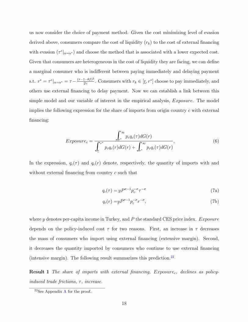
us now consider the choice of payment method. Given the cost minimizing level of evasion
derived above, consumers compare the cost of liquidity (rk) to the cost of external financing
with evasion (τ e|α=α∗) and choose the method that is associated with a lower expected cost.
Given that consumers are heterogeneous in the cost of liquidity they are facing, we can define
a marginal consumer who is indifferent between paying immediately and delaying payment
s.t. r∗ = τ e|α=α∗ = τ− (τ−1−θf)2
2γ. Consumers with rk ∈ [r, r∗] choose to pay immediately, and
others use external financing to delay payment. Now we can establish a link between this
simple model and our variable of interest in the empirical analysis, Exposure. The model
implies the following expression for the share of imports from origin country c with external
financing:
Exposurec =
∫∞
r∗pcqc(τ)dG(r)∫
r∗
rpcqc(r)dG(r) +
∫∞
r∗pcqc(τ)dG(r)
, (6)
In the expression, qc(τ) and qc(r) denote, respectively, the quantity of imports with and
without external financing from country c such that
qc(τ) = yP σ−1p−σc τ−σ (7a)
qc(r) =yP σ−1p−σc r−σ, (7b)
where y denotes per-capita income in Turkey, and P the standard CES price index. Exposure
depends on the policy-induced cost τ for two reasons. First, an increase in τ decreases
the mass of consumers who import using external financing (extensive margin). Second,
it decreases the quantity imported by consumers who continue to use external financing
(intensive margin). The following result summarizes this prediction.22
Result 1 The share of imports with external financing, Exposurec, declines as policy-
induced trade frictions, τ , increase.
22See Appendix A for the proof.
18

This result highlights the importance of taking the nature of the policy into account when
evaluating its impact. In particular, the extent to which changes in the policy-induced tax
rate τ affect imports is determined by the choices made by individual importers. Therefore,
differences in the behavior of importers create a new extensive margin of adjustment, which
is captured by Exposure. Next, we consider the elasticity of firm imports with respect to
the tax rate. Demand for imports by firms that choose to pay immediately does not depend
on the tax rate. So, we focus on equation (7a) describing the behavior of firms that delay
payments. Taking the logarithm of both sides of the equation and replacing τ with τ e yield:
ln qc(τ) = ln(yP σ−1
)− σ ln pc − σ ln τ e (8)
It is easy to see that the elasticity of imports with respect to the evasion-inclusive tax rate
is equal to the price elasticity, which is given by σ. However, since we never observe the
evasion-inclusive tax rate, we need to derive the elasticity with respect to the policy rate, τ .
Using the expression for τ e, we can write the following relationship between ln τ e and ln τ :
ln τ e = ln τ + ln
(1− (τ − 1− θf)2
2γτ
)
Substituting this into the demand equation in (8) gives:
ln qc(τ) = ln(yP σ−1
)− σ ln pc − σ ln τ − σ ln
(1− (τ − 1− θf)2
2γτ
)
We can use this equation to estimate the tax elasticity of imports as follows:
ln qkc = β0 + β1 ln pkc + β2 ln τ + δc + δk + ekc, (9)
where δc absorbs the market specific variables ln (yP σ−1), and δk controls for selection into
external financing as only importers that face relatively high liquidity costs, such that rk > r∗,
19

rely on external financing and delay payment. Since we cannot observe the evasion-inclusive
tax rate, ekc includes the term Ξ(τ) = −σ ln(
1− (τ−1−θf)2
2γτ
), which is positively correlated
with the policy tax rate:
dΞ
dτ=
σ
2(
1− (τ−1−θf)2
2γτ
) τ + 1 + θf
τ 2α∗ > 0
This creates a positive bias in the estimate of β2 as we expect β2 < 0.
Result 2 The elasticity of imports with respect to the evasion-inclusive tax rate is equal to
the price elasticity of demand for imports (ε), which is given by σ. Since the evasion-inclusive
tax rate is not observed, the elasticity with respect to the actual policy rate is estimated with
a positive bias, ετ > ε = −σ.
Put simply, a reduction in prices should generate a response in quantities as reflected by
σ. But if the reduction in prices is fake, i.e., driven by underreporting, a corresponding rise
in quantities will not be observed. A smaller or perhaps no response in quantities will be
registered.
Equation (9) forms the basis of our estimation strategy. We augment this equation by
including a time subscript. We focus on ordinary import flows. We estimate the equation
using firm-product-country-level import data disaggregated by financing terms.
In the estimation, we need to address a number of issues. First, equation (9) is subject to
the classical endogeneity bias associated with demand estimation. To address this problem,
we use the distance between the importing firm and the source country as an instrument for
import prices. More specifically, our instrument lnDistanceic is the logarithm of the sum
of the distance between the province in which the importing firm i is located and Istanbul
(the largest international port of Turkey) and the distance between Istanbul and country
c. Suppose that there are two firms importing the same product from the same country
through Istanbul. Our identification strategy relies on the fact that the one that is located
farther away from Istanbul will pay a higher c.i.f. price as it pays a higher domestic transport
20
cost. In other words, the instrument captures variation in transport costs, which affects the
quantity demanded only through its effect on cif prices. Second, while the model does not
distinguish between different products, one could expect heterogeneity across products within
a country in the data. We address this issue by adding fixed effects at the source-country-
6-digit-product-time level. Third, we add firm-time fixed effects to control for potential
time-varying confounding factors at the firm level, as well as to account for selection into
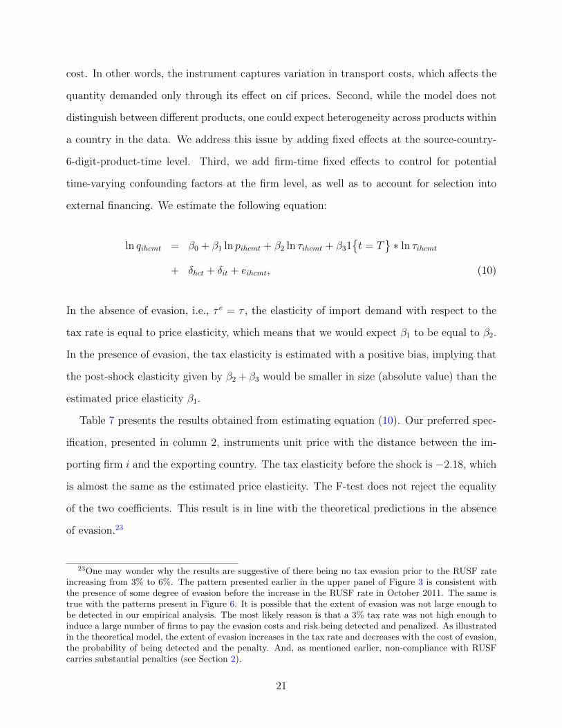
external financing. We estimate the following equation:
ln qihcmt = β0 + β1 ln pihcmt + β2 ln τihcmt + β31{t = T
}∗ ln τihcmt
+ δhct + δit + eihcmt, (10)
In the absence of evasion, i.e., τ e = τ , the elasticity of import demand with respect to the
tax rate is equal to price elasticity, which means that we would expect β1 to be equal to β2.
In the presence of evasion, the tax elasticity is estimated with a positive bias, implying that
the post-shock elasticity given by β2 + β3 would be smaller in size (absolute value) than the
estimated price elasticity β1.
Table 7 presents the results obtained from estimating equation (10). Our preferred spec-
ification, presented in column 2, instruments unit price with the distance between the im-
porting firm i and the exporting country. The tax elasticity before the shock is −2.18, which
is almost the same as the estimated price elasticity. The F-test does not reject the equality
of the two coefficients. This result is in line with the theoretical predictions in the absence
of evasion.23
23One may wonder why the results are suggestive of there being no tax evasion prior to the RUSF rateincreasing from 3% to 6%. The pattern presented earlier in the upper panel of Figure 3 is consistent withthe presence of some degree of evasion before the increase in the RUSF rate in October 2011. The same istrue with the patterns present in Figure 6. It is possible that the extent of evasion was not large enough tobe detected in our empirical analysis. The most likely reason is that a 3% tax rate was not high enough toinduce a large number of firms to pay the evasion costs and risk being detected and penalized. As illustratedin the theoretical model, the extent of evasion increases in the tax rate and decreases with the cost of evasion,the probability of being detected and the penalty. And, as mentioned earlier, non-compliance with RUSFcarries substantial penalties (see Section 2).
21
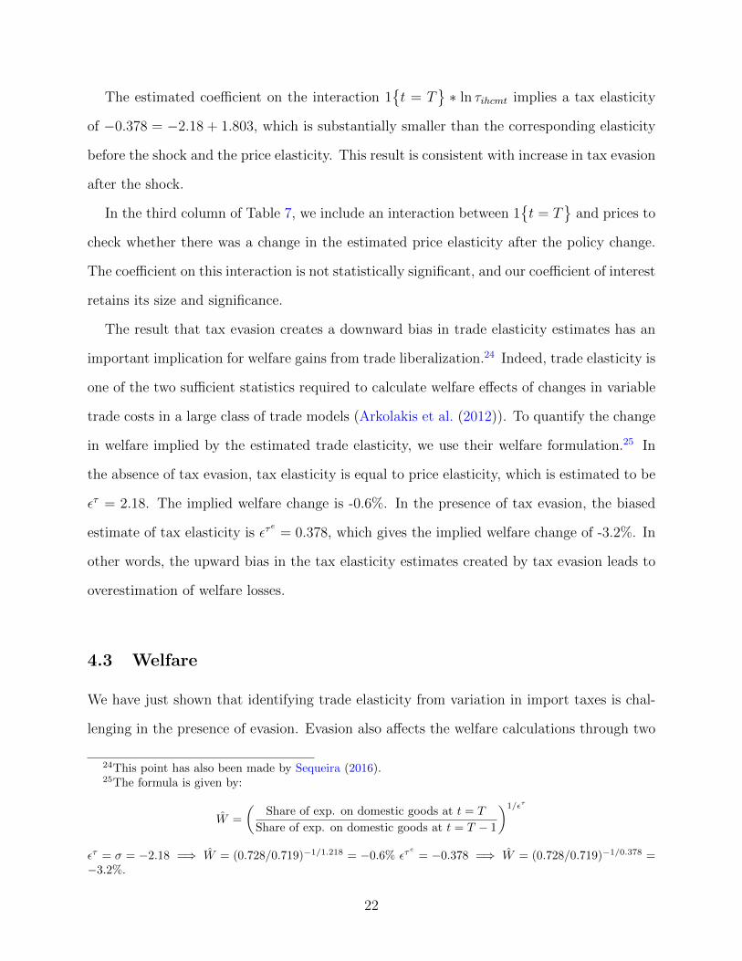
The estimated coefficient on the interaction 1{t = T
}∗ ln τihcmt implies a tax elasticity
of −0.378 = −2.18 + 1.803, which is substantially smaller than the corresponding elasticity
before the shock and the price elasticity. This result is consistent with increase in tax evasion
after the shock.
In the third column of Table 7, we include an interaction between 1{t = T
}and prices to
check whether there was a change in the estimated price elasticity after the policy change.
The coefficient on this interaction is not statistically significant, and our coefficient of interest
retains its size and significance.
The result that tax evasion creates a downward bias in trade elasticity estimates has an
important implication for welfare gains from trade liberalization.24 Indeed, trade elasticity is
one of the two sufficient statistics required to calculate welfare effects of changes in variable
trade costs in a large class of trade models (Arkolakis et al. (2012)). To quantify the change
in welfare implied by the estimated trade elasticity, we use their welfare formulation.25 In
the absence of tax evasion, tax elasticity is equal to price elasticity, which is estimated to be
ετ = 2.18. The implied welfare change is -0.6%. In the presence of tax evasion, the biased
estimate of tax elasticity is ετe
= 0.378, which gives the implied welfare change of -3.2%. In
other words, the upward bias in the tax elasticity estimates created by tax evasion leads to
overestimation of welfare losses.
4.3 Welfare
We have just shown that identifying trade elasticity from variation in import taxes is chal-
lenging in the presence of evasion. Evasion also affects the welfare calculations through two
24This point has also been made by Sequeira (2016).25The formula is given by:
W =
(Share of exp. on domestic goods at t = T
Share of exp. on domestic goods at t = T − 1
)1/ετ
ετ = σ = −2.18 =⇒ W = (0.728/0.719)−1/1.218 = −0.6% ετe
= −0.378 =⇒ W = (0.728/0.719)−1/0.378 =−3.2%.
22
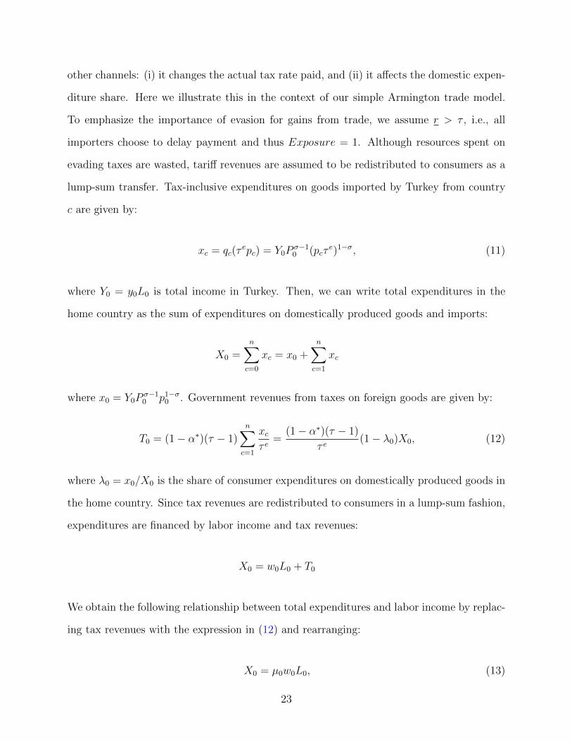
other channels: (i) it changes the actual tax rate paid, and (ii) it affects the domestic expen-
diture share. Here we illustrate this in the context of our simple Armington trade model.
To emphasize the importance of evasion for gains from trade, we assume r > τ , i.e., all
importers choose to delay payment and thus Exposure = 1. Although resources spent on
evading taxes are wasted, tariff revenues are assumed to be redistributed to consumers as a
lump-sum transfer. Tax-inclusive expenditures on goods imported by Turkey from country
c are given by:
xc = qc(τepc) = Y0P
σ−10 (pcτ
e)1−σ, (11)
where Y0 = y0L0 is total income in Turkey. Then, we can write total expenditures in the
home country as the sum of expenditures on domestically produced goods and imports:
X0 =n∑c=0
xc = x0 +n∑c=1
xc
where x0 = Y0Pσ−10 p1−σ
0 . Government revenues from taxes on foreign goods are given by:
T0 = (1− α∗)(τ − 1)n∑c=1
xcτ e
=(1− α∗)(τ − 1)
τ e(1− λ0)X0, (12)
where λ0 = x0/X0 is the share of consumer expenditures on domestically produced goods in
the home country. Since tax revenues are redistributed to consumers in a lump-sum fashion,
expenditures are financed by labor income and tax revenues:
X0 = w0L0 + T0
We obtain the following relationship between total expenditures and labor income by replac-
ing tax revenues with the expression in (12) and rearranging:
X0 = µ0w0L0, (13)
23
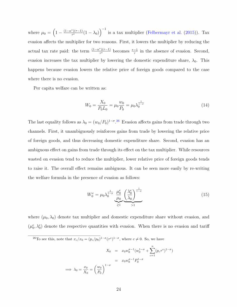
where µ0 =(
1− (1−α∗)(τ−1)τe
(1− λ0))−1
is a tax multiplier (Felbermayr et al. (2015)). Tax
evasion affects the multiplier for two reasons. First, it lowers the multiplier by reducing the
actual tax rate paid: the term (1−α∗)(τ−1)τe
becomes τ−1τ
in the absence of evasion. Second,
evasion increases the tax multiplier by lowering the domestic expenditure share, λ0. This
happens because evasion lowers the relative price of foreign goods compared to the case
where there is no evasion.
Per capita welfare can be written as:
W0 =X0
P0L0
= µ0w0
P0
= µ0λ1
1−σ0 (14)
The last equality follows as λ0 = (w0/P0)1−σ.26 Evasion affects gains from trade through two
channels. First, it unambiguously reinforces gains from trade by lowering the relative price
of foreign goods, and thus decreasing domestic expenditure share. Second, evasion has an
ambiguous effect on gains from trade through its effect on the tax multiplier. While resources
wasted on evasion tend to reduce the multiplier, lower relative price of foreign goods tends
to raise it. The overall effect remains ambiguous. It can be seen more easily by re-writing
the welfare formula in the presence of evasion as follows:
W e0 = µ0λ
11−σ0
µe0µ0︸︷︷︸≷1
(λe0λ0
) 11−σ
︸ ︷︷ ︸>1
(15)
where (µ0, λ0) denote tax multiplier and domestic expenditure share without evasion, and
(µe0, λe0) denote the respective quantities with evasion. When there is no evasion and tariff
26To see this, note that xc/x0 = (pc/p0)1−σ(τe)1−σ, where c 6= 0. So, we have
X0 = x0wσ−10 (w1−σ
0 +
n∑c=1
(pcτe)1−σ)
= x0wσ−10 P 1−σ
0
=⇒ λ0 =x0X0
=
(w0
P0
)1−σ
24
revenues are wasted, the welfare formula in (15) collapses to the one in Arkolakis et al.
(2012). The last two terms arise due to evasion. The expression in (15) implies tax evasion
unambiguously reinforces gains from trade when tariff revenues are wasted instead of being
redistributed to consumers: µe0 = µ0 = 1. In this case, tariff evasion affects welfare only
through its effect on the domestic expenditure share. Since tax evasion unambiguously
lowers the domestic expenditure share, tax evasion reinforces gains from trade.
5 Conclusions
This paper proposes two novel methods of detecting tax evasion in international trade. The
first method uses deviations from Benford’s law, while the second method relies on comparing
price and trade cost elasticity of import demand. We apply both methods to an unexpected
policy change that increased the cost of import financing in Turkey and show that both
methods produce evidence consistent with an increase in tax evasion after the shock. A
standard approach based on “missing trade” confirms this conclusion. Our results also
suggest that ignoring tax evasion may lead to miscalculation of gains from changing trade
barriers based on standard welfare formulations. Finally, we derive formula to calculate gains
from trade in a simple Armington trade model with tax evasion.
25
References
Arkolakis, Costas, Arnaud Costinot, and Andres Rodriguez-Clare, “New Trade
Models, Same Old Gains?,” American Economic Review, February 2012, 102 (1), 94–130.
Artavanis, Nikolaos, Adair Morse, and Margarita Tsoutsoura, “Measuring Income
Tax Evasion Using Bank Credit: Evidence from Greece *,” The Quarterly Journal of
Economics, 2016, 131 (2), 739–798.
Baier, Scott L. and Jeffrey H. Bergstrand, “The growth of world trade: tariffs, trans-
port costs, and income similarity,” Journal of International Economics, 2001, 53 (1), 1 –
27.
Bhagwati, Jagdish N., “Directly-unproductive, profit-seeking activities: welfare-theoretic
synthesis and generalization,” Journal of Political Economy, October 1982, 90.
and T. N. Srinivasan, “The welfare consequences of directly-unproductive profit-
seeking (DUP) lobbying activities : Price versus quantity distortions,” Journal of In-
ternational Economics, August 1982, 13 (1-2), 33–44.
Camerer, C., Behavioral Game Theory : Experiments in Strategic Interaction, New Age
International, 2003.
Casaburi, Lorenzo and Ugo Troiano, “Ghost-House Busters: The Electoral Response
to a Large AntiTax Evasion Program,” The Quarterly Journal of Economics, 2016, 131
(1), 273–314.
Chen, Zhao, Zhikuo Liu, Juan Carlos Suarez Serrato, and Daniel Xu, “Notching
R&D Investment with Corporate Income Tax Cuts in China,” Mimeo, Department of
Economics, University of Duke 2017.
Cho, Wendy K Tam and Brian J Gaines, “Breaking the (Benford) Law,” The American
Statistician, 2007, 61 (3), 218–223.
26
Durtschi, Cindy, William Hillison, and Carl Pacini, “Effective Use of Benford’s Law
to Assist in Detecting Fraud in Accounting Data,” Journal of Forensic Accounting, 2004,
4.
EY, “TradeWatch, March 2014,” 2014. http://www.ey.com/Publication/vwLUAssets/
EY-tradewatch-vol13-issue1/$FILE/EY-tradewatch-Vol13-Issue1.pdf.
Fang, Hanming and Qing Gong, “Detecting Potential Overbilling in Medicare Reim-
bursement via Hours Worked,” American Economic Review, February 2017, 107 (2), 562–
91.
Feenstra, Robert C., “Chapter 30 Estimating the effects of trade policy,” in “,” Vol. 3 of
Handbook of International Economics, Elsevier, 1995, pp. 1553 – 1595.
Felbermayr, Gabriel, Benjamin Jung, and Mario Larch, “The welfare consequences
of import tariffs: A quantitative perspective,” Journal of International Economics, 2015,
97 (2), 295–309.
Ferrantino, Michael J., Xuepeng Liu, and Zhi Wang, “Evasion behaviors of exporters
and importers: Evidence from the U.S.China trade data discrepancy,” Journal of Inter-
national Economics, 2012, 86 (1), 141–157.
Fisman, Raymond and Shang-Jin Wei, “Tax Rates and Tax Evasion: Evidence from
“Missing Imports in China,” Journal of Political Economy, April 2004, 112 (2), 471–500.
, Peter Moustakerski, and Shang-Jin Wei, “Outsourcing Tariff Evasion: A New
Explanation for Entrept Trade,” The Review of Economics and Statistics, 2008, 90 (3),
587–592.
Goldberg, Pinelopi K. and Nina Pavcnik, “The Effects of Trade Policy,” NBER Work-
ing Papers 21957, National Bureau of Economic Research, Inc February 2016.
27

Han, Chang-Ryung, “A Survey of Customs Administration Perceptions on Illegal Trade,”
WCO Research Paper 34, World Customs Organization 2014.
Hill, Theodore P., “A Statistical Derivation of the Significant-Digit LawDetecting Prob-
lems in Survey Data Using Benfords Law,” Statistical Science, 1995, 4.
, “The Difficulty of Faking Data,” CHANCE, 1999, 12 (3), 27–31.
Javorcik, Beata S. and Gaia Narciso, “Differentiated products and evasion of import
tariffs,” Journal of International Economics, December 2008, 76 (2), 208–222.
and , “WTO accession and tariff evasion,” Journal of Development Economics, 2017,
125, 59 – 71.
Judge, George and Laura Schechter, “Detecting Problems in Survey Data Using Ben-
fords Law,” Journal of Human Resources, 2009, 44 (1).
Marion, Justin and Erich Muehlegger, “Measuring Illegal Activity and the Effects
of Regulatory Innovation: Tax Evasion and the Dyeing of Untaxed Diesel,” Journal of
Political Economy, 2008, 116 (4), 633–666.
Michalski, Tomasz and Gilles Stoltz, “Do Countries Falsify Economic Data Strategi-
cally? Some Evidence That They Might,” The Review of Economics and Statistics, May
2013, 95 (2), 591–616.
Mishra, Prachi, Arvind Subramanian, and Petia Topalova, “Tariffs, enforcement,
and customs evasion: Evidence from India,” Journal of Public Economics, 2008, 92 (1011),
1907 – 1925.
Sequeira, Sandra, “Corruption, Trade Costs, and Gains from Tariff Liberalization: Evi-
dence from Southern Africa,” American Economic Review, October 2016, 106 (10), 3029–
3063.
28
Trefler, Daniel, “The Long and Short of the Canada-U. S. Free Trade Agreement,” Amer-
ican Economic Review, September 2004, 94 (4), 870–895.
Yang, Dean, “Can Enforcement Backfire? Crime Displacement in the Context of Customs
Reform in the Philippines,” The Review of Economics and Statistics, February 2008, 90
(1), 1–14.
29
Appendices
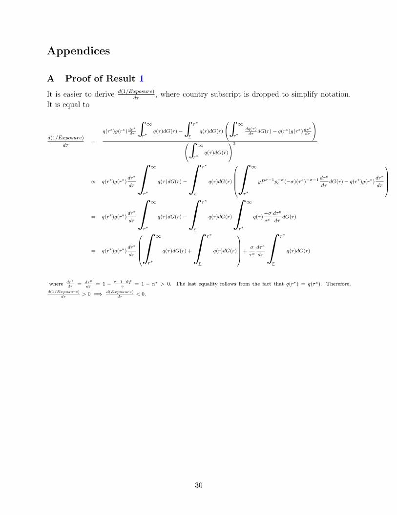
A Proof of Result 1
It is easier to derive d(1/Exposure)dτ
, where country subscript is dropped to simplify notation.
It is equal to
d(1/Exposure)
dτ=
q(r∗)g(r∗) dr∗
dτ
∫∞
r∗q(τ)dG(r)−
∫r∗
rq(r)dG(r)
∫∞
r∗dq(τ)dτ
dG(r)− q(r∗)g(r∗) dr∗
dτ
∫∞
r∗q(τ)dG(r)
2
∝ q(r∗)g(r∗)dr∗
dτ
∫∞
r∗
q(τ)dG(r)−
∫r∗
r
q(r)dG(r)
∫
∞
r∗
yPσ−1p−σc (−σ)(τe)−σ−1 dτe
dτdG(r)− q(r∗)g(r∗)
dr∗
dτ
= q(r∗)g(r∗)dr∗
dτ
∫∞
r∗
q(τ)dG(r)−
∫r∗
r
q(r)dG(r)
∫∞
r∗
q(τ)−στe
dτe
dτdG(r)
= q(r∗)g(r∗)dr∗
dτ
∫
∞
r∗
q(τ)dG(r) +
∫r∗
r
q(r)dG(r)
+σ
τedτe
dτ
∫r∗
r
q(r)dG(r)
where dr∗
dτ= dτe
dτ= 1 − τ−1−θf
γ= 1 − α∗ > 0. The last equality follows from the fact that q(r∗) = q(τe). Therefore,
d(1/Exposure)dτ
> 0 =⇒ d(Exposure)dτ
< 0.
30
B Tables and Figures
Table 1: Firm-level Imports before and after the Shock
Baseline Pre-existing trends Processing imports
(1) (2) (3)
1{t = T
}∗ Exposurei,T−2 -0.119∗∗ -0.151∗∗ -0.104
(0.0530) (0.0665) (0.0847)
1{t = T − 1
}∗ Exposurei,T−2 -0.0666
(0.0640)
N 45818 45818 8549
R2 0.888 0.888 0.910
Fixed effects s(i)xt,i s(i)xt,i s(i)xt,i
Notes: This table shows the results from estimating the following regression:
lnMit = δ0 + δ11{t = T
}∗ Exposurei,T−2 + αs(i),t + αi + eit
where the dependent variable is the logarithm of the value of imports by firm i at time t = {T −2, T −1, T},
and Exposurei,T−2 is share of firm-level imports with external financing at time t = T − 2. 1{t = T
}is a
dummy variable that takes on the value one for the October 2011-September 2012 period (after the increase
in RUSF rate), and zero otherwise. The specification controls for time-varying factors common to a given
4-digit NACE industry (αs(i),t) and firm fixed effects (αi).*, **, *** represent significance at the 10, 5, and 1
percent levels, respectively. Robust standard errors (in parentheses) are clustered at the the 4-digit NACE
industry where firm i operates.
31
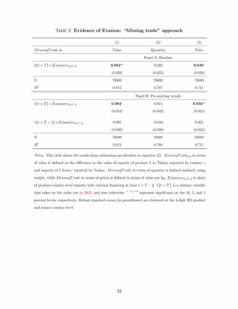
Table 2: Evidence of Evasion: “Missing trade” approach
(1) (2) (3)
MissingTrade in Value Quantity Price
Panel A: Baseline
1{t = T} ∗ Exposurehc,T−2 0.062∗∗ 0.022 0.040∗
(0.028) (0.035) (0.020)
N 70089 70089 70089
R2 0.812 0.787 0.711
Panel B: Pre-existing trends
1{t = T} ∗ Exposurehc,T−2 0.064∗ 0.014 0.050∗∗
(0.034) (0.042) (0.025)
1{t = T − 1} ∗ Exposurehc,T−2 0.005 -0.016 0.021
(0.030) (0.038) (0.024)
N 70089 70089 70089
R2 0.812 0.788 0.711
Notes: This table shows the results from estimating specification in equation (2). MissingTradehct in terms
of value is defined as the difference in the value of exports of product h to Turkey reported by country c
and imports of h from c reported by Turkey. MissingTrade in terms of quantity is defined similarly using
weight, while MissingTrade in terms of prices is defined in terms of value per kg. Exposurehc,T−2 is share
of product-country-level imports with external financing at time t = T − 2. 1{t = T
}is a dummy variable
that takes on the value one in 2012, and zero otherwise. *, **, *** represent significance at the 10, 5, and 1
percent levels, respectively. Robust standard errors (in parentheses) are clustered at the 4-digit HS product
and source country level.
32
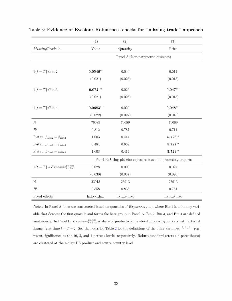
Table 3: Evidence of Evasion: Robustness checks for “missing trade” approach
(1) (2) (3)
MissingTrade in Value Quantity Price
Panel A: Non-parametric estimates
1{t = T}∗Bin 2 0.0546∗∗ 0.040 0.014
(0.021) (0.026) (0.015)
1{t = T}∗Bin 3 0.072∗∗∗ 0.026 0.047∗∗∗
(0.021) (0.026) (0.015)
1{t = T}∗Bin 4 0.0683∗∗∗ 0.020 0.048∗∗∗
(0.022) (0.027) (0.015)
N 70089 70089 70089
R2 0.812 0.787 0.711
F-stat. βBin2 = βBin3 1.003 0.414 5.723∗∗
F-stat. βBin2 = βBin4 0.484 0.659 5.727∗∗
F-stat. βBin3 = βBin4 1.003 0.414 5.723∗∗
Panel B: Using placebo exposure based on processing imports
1{t = T} ∗ Exposureplacebohc,T−2 0.028 0.000 0.027
(0.030) (0.037) (0.020)
N 23913 23913 23913
R2 0.858 0.838 0.761
Fixed effects hxt,cxt,hxc hxt,cxt,hxc hxt,cxt,hxc
Notes: In Panel A, bins are constructed based on quartiles of Exposurehc,T−2, where Bin 1 is a dummy vari-
able that denotes the first quartile and forms the base group in Panel A. Bin 2, Bin 3, and Bin 4 are defined
analogously. In Panel B, Exposureplacebohc,T−2 is share of product-country-level processing imports with external
financing at time t = T − 2. See the notes for Table 2 for the definitions of the other variables. *, **, *** rep-
resent significance at the 10, 5, and 1 percent levels, respectively. Robust standard errors (in parentheses)
are clustered at the 4-digit HS product and source country level.
33
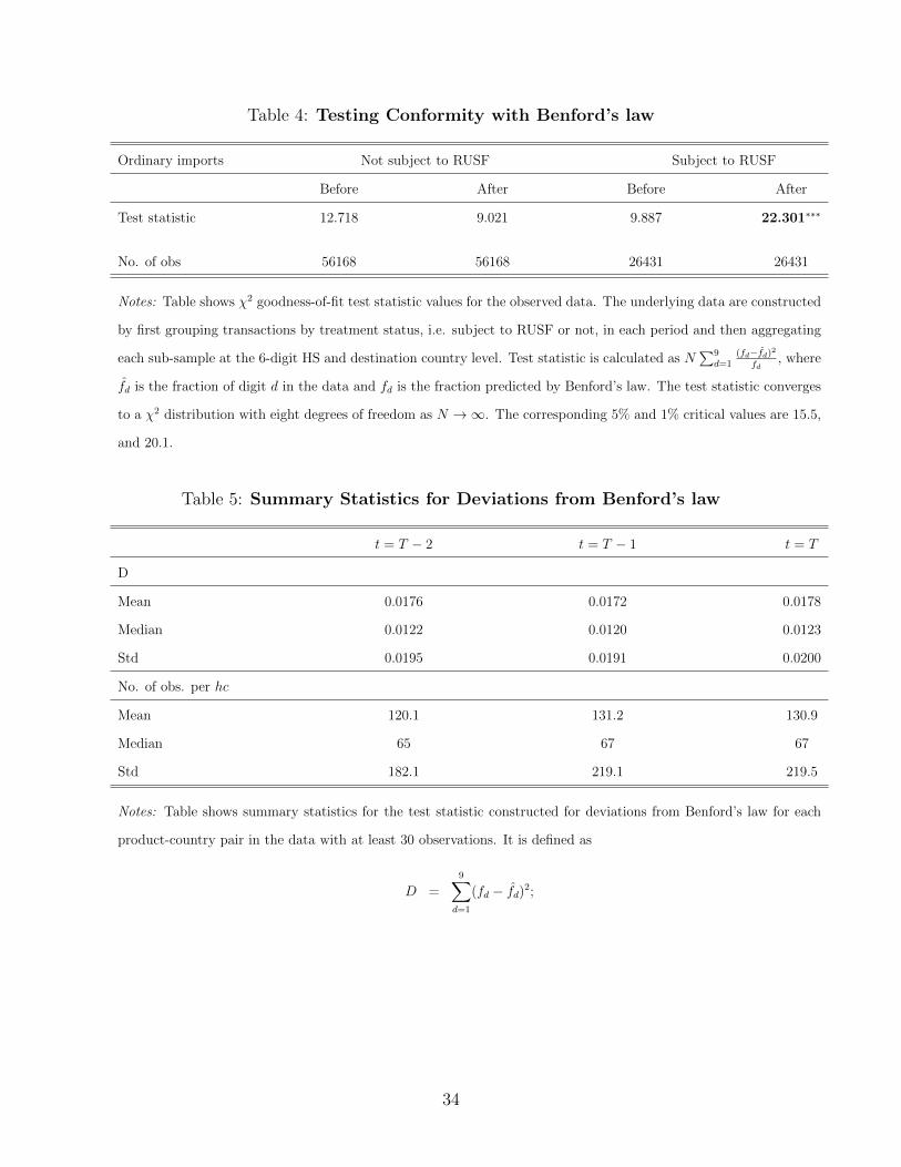
Table 4: Testing Conformity with Benford’s law
Ordinary imports Not subject to RUSF Subject to RUSF
Before After Before After
Test statistic 12.718 9.021 9.887 22.301∗∗∗
No. of obs 56168 56168 26431 26431
Notes: Table shows χ2 goodness-of-fit test statistic values for the observed data. The underlying data are constructed
by first grouping transactions by treatment status, i.e. subject to RUSF or not, in each period and then aggregating
each sub-sample at the 6-digit HS and destination country level. Test statistic is calculated as N∑9
d=1(fd−fd)2
fd, where
fd is the fraction of digit d in the data and fd is the fraction predicted by Benford’s law. The test statistic converges
to a χ2 distribution with eight degrees of freedom as N →∞. The corresponding 5% and 1% critical values are 15.5,
and 20.1.
Table 5: Summary Statistics for Deviations from Benford’s law
t = T − 2 t = T − 1 t = T
D
Mean 0.0176 0.0172 0.0178
Median 0.0122 0.0120 0.0123
Std 0.0195 0.0191 0.0200
No. of obs. per hc
Mean 120.1 131.2 130.9
Median 65 67 67
Std 182.1 219.1 219.5
Notes: Table shows summary statistics for the test statistic constructed for deviations from Benford’s law for each
product-country pair in the data with at least 30 observations. It is defined as
D =9∑d=1
(fd − fd)2;
34
Tab
le6:
Evid
ence
of
Evasi
on:
Usi
ng
Benfo
rd’s
law
(1)
(2)
(3)
(4)
(5)
Bas
elin
eP
re-e
xis
ting
tren
ds
Fir
sttw
odig
its
Fir
stth
ree
dig
its
Pro
cess
ing
1{t
=T}∗Exposurehc,T−
20.0
0286∗∗∗
0.0
0228∗
0.0
00694∗
0.0
00376∗∗∗
0.00
0081
1
(0.0
0107
)(0
.001
37)
(0.0
0037
4)(0
.000
110)
(0.0
0071
9)
1{t
=T−
1}∗Exposurehc,T−
2-0
.000
970
(0.0
0130
)
N26
369
2636
926
369
2636
912
468
R2
0.76
60.
766
0.88
20.
955
0.79
8
Fix
edeff
ects
hxt,
cxt,
hxc
hxt,
cxt,
hxc
hxt,
cxt,
hxc
hxt,
cxt,
hxc
hxt,
cxt,
hxc
Not
es:
This
table
show
sth
ere
sult
sfr
omes
tim
atin
gsp
ecifi
cati
onin
equat
ion
(5).
Inal
lco
lum
ns
(exce
pt
colu
mns
3-4)
the
dep
enden
tva
riab
leisDhct
,w
hic
hm
easu
res
for
each
hc-
pai
rth
edev
iati
onof
obse
rved
dis
trib
uti
onfr
omB
enfo
rd’s
law
defi
ned
as:
Dhct
=9 ∑ d=
1
(fd hct−fd hct
)2.
Inco
lum
ns
3-4,
the
dep
enden
tva
riab
lem
easu
res
the
dev
iati
ons
ofth
ejo
int
dis
trib
uti
onof
the
lead
ingk
dig
its
from
the
pre
dic
ted
dis
trib
uti
onby
Ben
ford
law
whic
his
give
nby:
Prob(D
1=d
1,...,D
k=dk)
=log 1
0
1+( k ∑ i=
1
di∗
10k−i) −1 ,
wher
ek
=1,
2,3.Exposurehc,T−
2is
shar
eof
pro
duct
-cou
ntr
y-l
evel
imp
orts
wit
hex
tern
alfinan
cing
atti
met
=T−
2.1{ t=
T} is
adum
my
vari
able
that
take
son
the
valu
e
one
for
the
Oct
ober
2011
-Sep
tem
ber
2012
per
iod,
and
zero
other
wis
e.*,
**,
***
repre
sent
sign
ifica
nce
atth
e10
,5,
and
1p
erce
nt
leve
ls,
resp
ecti
vely
.R
obust
stan
dar
der
rors
(in
par
enth
eses
)ar
ecl
ust
ered
atth
e4-
dig
itH
Spro
duct
and
sourc
eco
untr
yle
vel.
35
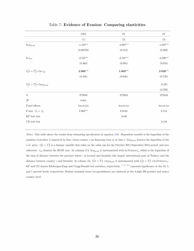
Table 7: Evidence of Evasion: Comparing elasticities
OLS IV IV
(1) (2) (3)
ln pihcmt -1.163∗∗∗ -2.065∗∗∗ -1.937∗∗∗
(0.00729) (0.412) (0.389)
ln τmt -2.545∗∗∗ -2.181∗∗∗ -2.296∗∗∗
(0.464) (0.691) (0.655)
1{t = T
}∗ ln τmt 2.008∗∗∗ 1.803∗∗∗ 2.026∗∗∗
(0.456) (0.640) (0.720)
1{t = T
}∗ ln pihcmt -0.325
(0.599)
N 875034 875034 875034
R2 0.841
Fixed effects hxcxt,ixt hxcxt,ixt hxcxt,ixt
F-stat. β1 = β2 8.903∗∗∗ 0.0144 0.154
KP test stat 14.08
CD test stat 11.94
Notes: This table shows the results from estimating specification in equation (10). Dependent variable is the logarithm of the
quantity of product h imported by firm i from country c on financing term m at time t. ln pihcmt denotes the logarithm of the
c.i.f. price. 1{t = T
}is a dummy variable that takes on the value one for the October 2011-September 2012 period, and zero
otherwise. τmt denotes the RUSF rate. In columns 2-3, ln pihcmt is instrumented with lnDistanceic which is the logarithm of
the sum of distance between the province where i is located and Istanbul (the largest international port of Turkey) and the
distance between country c and Istanbul. In column (3), 1{t = T
}∗ ln pihcmt is instrumented with 1
{t = T
}∗ lnDistanceic.
KP and CG denote Kleibergen-Paap and Cragg-Donald test statistics, respectively. *, **, *** represent significance at the 10, 5,
and 1 percent levels, respectively. Robust standard errors (in parentheses) are clustered at the 4-digit HS product and source
country level.
36
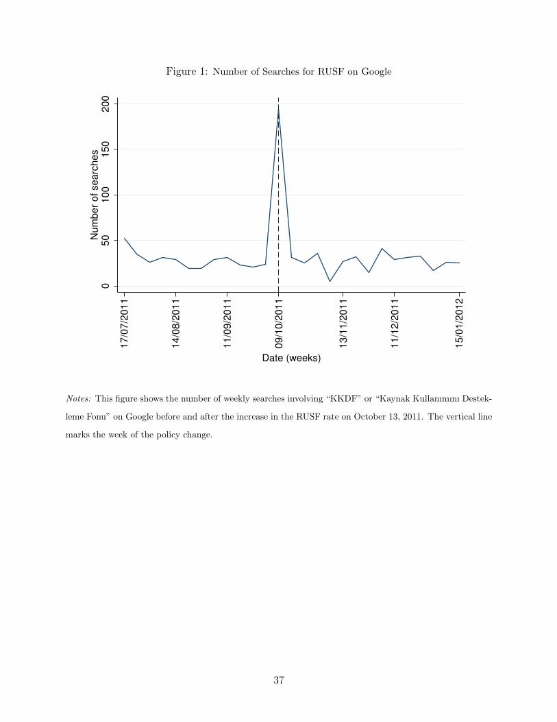
Figure 1: Number of Searches for RUSF on Google
05
01
00
15
02
00
Nu
mb
er
of
se
arc
he
s
17
/07
/20
11
14
/08
/20
11
11
/09
/20
11
09
/10
/20
11
13
/11
/20
11
11
/12
/20
11
15
/01
/20
12
Date (weeks)
Notes: This figure shows the number of weekly searches involving “KKDF” or “Kaynak Kullanımını Destek-
leme Fonu” on Google before and after the increase in the RUSF rate on October 13, 2011. The vertical line
marks the week of the policy change.
37
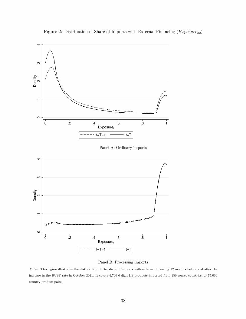
Figure 2: Distribution of Share of Imports with External Financing (Exposurehc)
01
23
4D
ensity
0 .2 .4 .6 .8 1Exposuret
t=T−1 t=T
Panel A: Ordinary imports
01
23
4D
ensity
0 .2 .4 .6 .8 1Exposuret
t=T−1 t=T
Panel B: Processing imports
Notes: This figure illustrates the distribution of the share of imports with external financing 12 months before and after the
increase in the RUSF rate in October 2011. It covers 4,700 6-digit HS products imported from 150 source countries, or 75,000
country-product pairs.
38
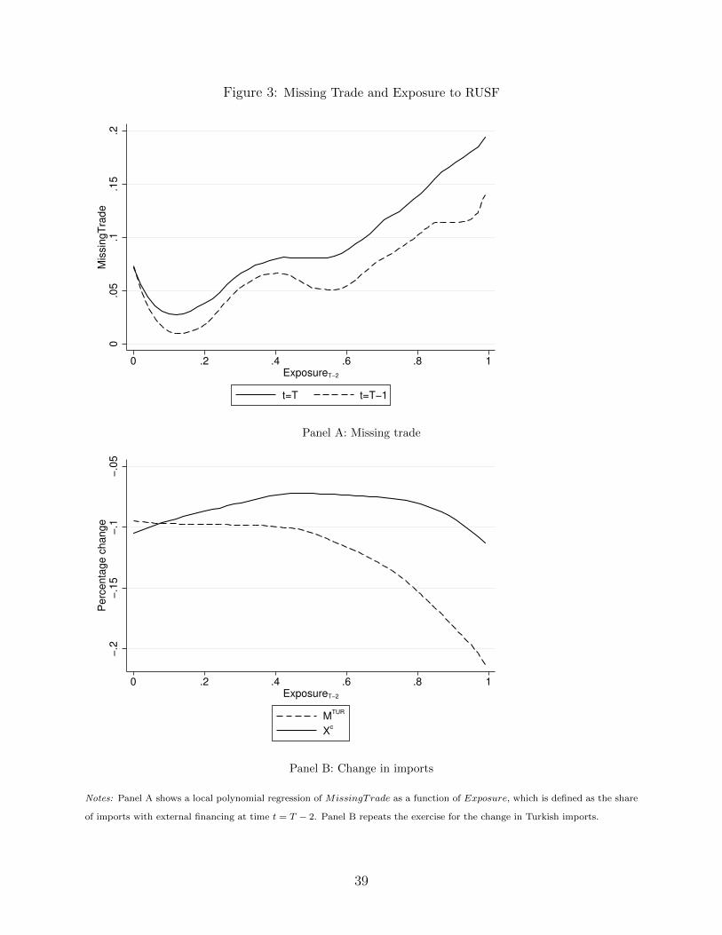
Figure 3: Missing Trade and Exposure to RUSF
0.0
5.1
.15
.2M
issin
gT
rade
0 .2 .4 .6 .8 1ExposureT−2
t=T t=T−1
Panel A: Missing trade
−.2
−.1
5−
.1−
.05
Perc
enta
ge c
hange
0 .2 .4 .6 .8 1ExposureT−2
MTUR
Xc
Panel B: Change in imports
Notes: Panel A shows a local polynomial regression of MissingTrade as a function of Exposure, which is defined as the share
of imports with external financing at time t = T − 2. Panel B repeats the exercise for the change in Turkish imports.
39
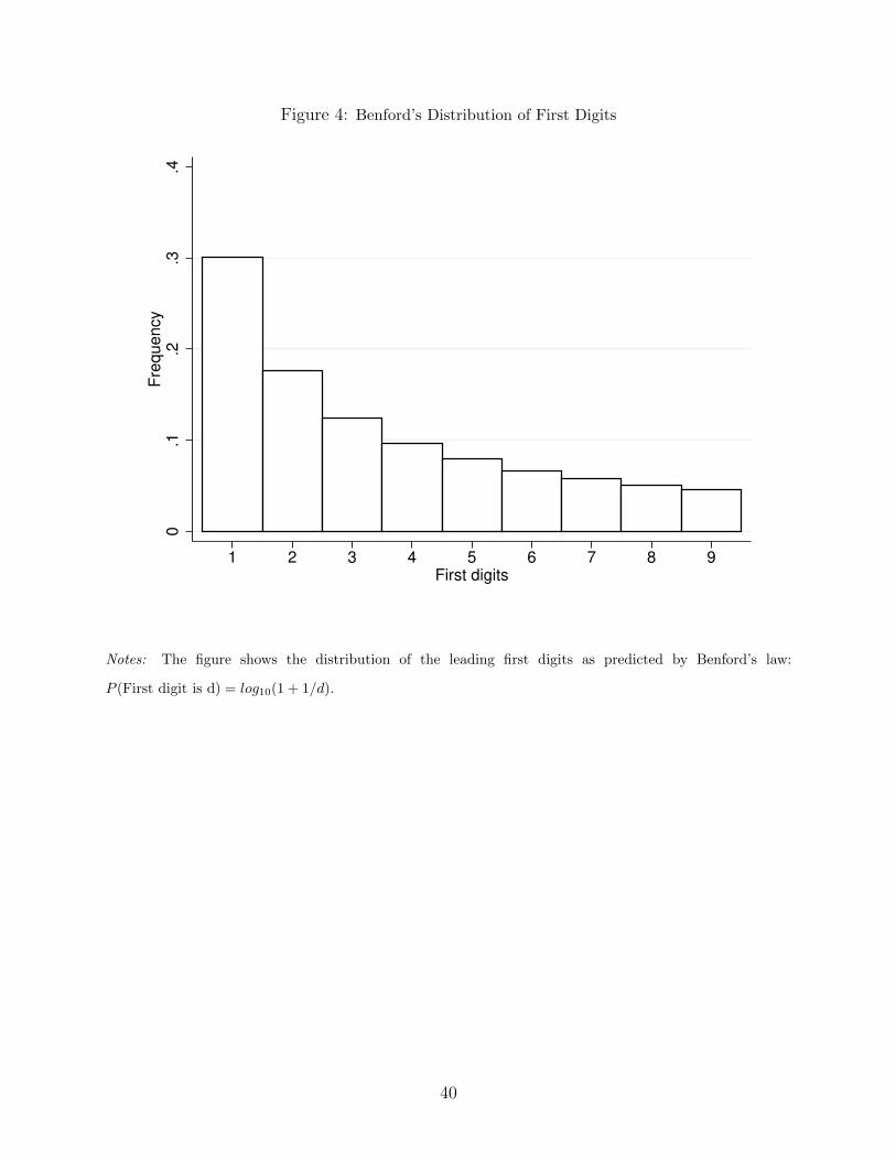
Figure 4: Benford’s Distribution of First Digits
0.1
.2.3
.4F
req
ue
ncy
1 2 3 4 5 6 7 8 9First digits
Notes: The figure shows the distribution of the leading first digits as predicted by Benford’s law:
P (First digit is d) = log10(1 + 1/d).
40
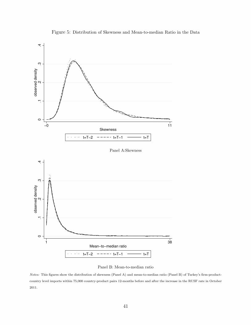
Figure 5: Distribution of Skewness and Mean-to-median Ratio in the Data
0.1
.2.3
.4observ
ed d
ensity
−0 11Skewness
t=T−2 t=T−1 t=T
Panel A:Skewness
0.1
.2.3
.4observ
ed d
ensity
1 38Mean−to−median ratio
t=T−2 t=T−1 t=T
Panel B: Mean-to-median ratio
Notes: This figures show the distribution of skewness (Panel A) and mean-to-median ratio (Panel B) of Turkey’s firm-product-
country level imports within 75,000 country-product pairs 12-months before and after the increase in the RUSF rate in October
2011.
41
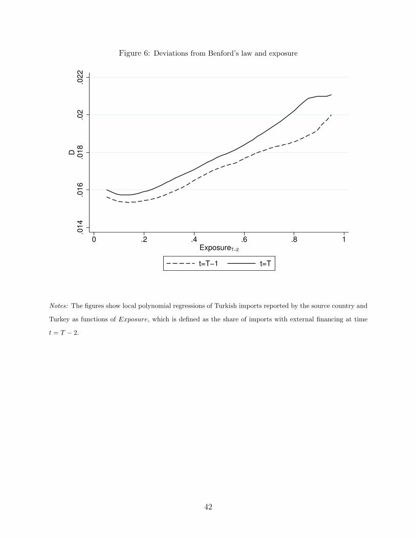
Figure 6: Deviations from Benford’s law and exposure
.01
4.0
16
.01
8.0
2.0
22
D
0 .2 .4 .6 .8 1ExposureT−2
t=T−1 t=T
Notes: The figures show local polynomial regressions of Turkish imports reported by the source country and
Turkey as functions of Exposure, which is defined as the share of imports with external financing at time
t = T − 2.
42