foreign assistance and korea's economic growth

FOREIGN ASSISTANCE AND KOREA’S ECONOMIC GROWTH

S. KIM University of Sydney

I. INTRODUCTION Korea has remained one of the principal recipients of foreign aid during the last

one and a half decades (1953-68). Cumulative aid between 1953, the year in which the Korean War ended, and 1966 reached 3 .2 billion United States dollars. This is comparable to the estimated loss of 3 billion United States dollars in the economy’s productive capacity during the Korean War’. Foreign aid has been, however, the main source of funds both for domestic capital formation and imports since 1953. The percentage shares of foreign savings in gross domestic capital formation and imports were respectively 74 per cent and 61 per cent on average since 1953. One would expect a foreign resource inflow of this magnitude to have had a major impact on the growth of the economy.

Between 1953 and 1966, the average annual growth rate of gross national product was 5 .4 per cent, while the population grew by 2.9 per cent per annum. The annual percentage share of foreign savings in gross domestic capital formation decreased

TABLE I Major Economic Performance Indicators of Developing Countries

Incremental Incremental GNP Growth Savings/GNP Capital/Output Export Growth

Country Rate Ratio Ratio Rate 1961-65 1963-67 1961-65 1963-67 1961-65 1963-67 1961-65 1963-67

China Thailand Greece Korea Mexico Malaysia Peru Pakistan Turkey Bolivia Philippines Ethiopia Tunisia Chile Colombia India Brazil Argentina

Arithmetical Average

9.3 11.5 7.8 7.8 7.7 7.7 7.6 9.8 7.1 7.1 6.2 6.4 6.1 5.3 6.0 5.4 5.8 6.8 5.4 6.0 4.9 4.7 4.6 4.4 4.6 2.7 4.5 4.7 4.3 4.5 4.1 1.8 3.1 4-2 2.6 4.3

5.6 5 . 8

0.41 0.35 0.39 0.32 0.31 0.14 0.31 0.34 0.24 0.23 0.06 0.28 0.10 0.30 0.04 -0.02 0.35 0.33 0.35 0.24 0.52 0.08 0.14 0.12 0.31 0.14 0.46 0.40 0.18 0.07 0.20 -0.28 0.01 -0.04 0.23 0.23

0.25 0.18

1.95 2.49 2.80 1.86 2,67 2.79 2.87 2.47 2.47 2.45 3.96 2.33 4.87 3.99 4.81 3.76 5-78 8.19

3.5

1.59 2.90 3.32 1.59 2.85 3.02 3.30 2.89 2.29 2.55 4.44 2.57 9-66 3.79 4.33 6.76 3.69 4.52

3.7

4.9 11-4 10-5 18.2 8-0 0.5 9.1 1.7 8.0

23.5 14.8 12.8 2.8

11.0 8.5 6.3 4-8 7.7

9.1

24.1 17.7 13.2 43.6 7.4 5 .5 8.8

11.4 12.0 17.4 9.5 6.7 6.3

10.9 -0.2 -1.5

6.0 3.0

11.2

Source: Derived from Yearbook of National Accounts Statistics, U.N., 1969, and Balance of Payments Yearbook, International Monetary Fund, 1969.

1 Sung-yu Hong, The Korean Economy and the American Aid (in Korean) (Seoul: Korea, 1962), p. 41.

90 AUSTRALIAN ECONOMIC PAPERS JUNE

from 117 per cent in 1953 to 41 per cent in 1966, indicating that capital formation was being increasingly financed from domestic savings. Exports increased by 18 per cent per annum during the period, contributing to a reduction in the share of foreign savings in imports from 83 per cent of 1953 to 42 per cent of 1966.

The contribution of foreign resources to economic growth has been more conspicuous in the later than in the earlier period in which resources were mainly allocated to post-war reconstruction. Economic performance was particularly impressive after 1961, when a military coup overthrew the existing government and the Second Republic was subsequently set up. A clearer evaluation can be made from Table I, which presents some indicators of the economic performance of 18 low-income countries all of which received foreign aid from economically advanced countries.

In the period 1961-65, the highest rate of growth per annum in gross national product was achieved by China (Taiwan), followed by Thailand and Greece. Korea’s rate of growth of 7.6 per cent per annum ranked fourth, a relatively satisfactory performance.

One of the factors contributing to the high rate of growth in Korea seems to be her relatively efficient utilisation of capital resources. Korea’s average gross capital- output ratio over the period was 1-86, which is the lowest ratio of all 18 countries under consideration, and compares particularly well with the Latin American and African countries. It is found that, in general, the size of the gross capital-output ratio is inversely related to the rate of growth of gross national product.

All of the 18 countries had positive values for the marginal savings-GNP ratio in the period. Korea’s ratio of 0.31 ranked sixth, but, compared to GNP growth performance, her savings drive was not so impressive.

The average annual rate of growth of total exports of the 18 countries was 9 - 1 per cent during the same period (1961-65). Korea, however, achieved a rate of 18.2 per cent per annum, which was second only to the Bolivian rate of 23.5 per cent. Con- sidering the stagnancy of exports between 1953 and 1961, this comparatively high rate of growth in Korea’s exports may be attributed to the significant growth of export- oriented industries, the bulk of the increment in exports being processed goods.

After 1963, Korea’s economic growth accelerated as shown by the 9.8 per cent annual rate of growth in gross national product, surpassed only by China’s 11 - 5 per cent rate of growth. Comparing the regional figures, we find that, except for the East Asian countries (China, Korea, Philippines and Thailand), the rate of growth in gross national product did not increase in other areas and even fell in the African, Near East and South Asian countries during this period. The gross capital-output ratio was still lowest in Korea, having fallen since the previous period. Korea’s marginal savings-GNP ratio rose from 0.31 to 0.34. Apparently she managed to allocated an increasing proportion of the increment in income generated by investment financed by the foreign resource inflow to the role of generating future income.

The most conspicuous progress, however, occurred in exports which increased by 43.6 per cent per annum in the second period. The average figure for the 18 countries was 11 -2 per cent per annum, a slightly higher figure than in the previous period. The continuous effort to industrialise before 1961 helped to increase exports, as after 1961 more than half of commodity exports were of manufactured products.

To sum up, the Korean economy performed relatively better than many other countries during the period 1957-68. Especially after 1961, the economy achieved accelerated growth in gross national product, savings and exports. The foreign resource transfer was utilised for post-war reconstruction in the earlier period but after 1961 was increasingly allocated to building up the capital stock, particularly social overhead

1972 FOREIGN ASSISTANCE AND KOREA’S ECONOMIC GROWTH 91

capital and manufacturing industries. Due to export-oriented industrialisation, manufactured exports have grown remarkably, while the growth of the gross national product has accelerated.

11. STATISTICAL MODEL In analysing the effects on economic growth of the foreign resource transfer, we will

regard foreign resources as a supplement to the resources at the economy’s disposal. Only foreign exchange resources and investment resources will be considered. Other resources, particularly human resources, including skill and managerial ability, are also important in the process of development, as is agreed upon by all students of economic development. Our analysis is limited, however, to the two resources because lack of data precludes any significant degree of quantitative analysis of the supply and use of other resources. Also, during the period covered by this analysis, the economy generally had an excess supply of human resources other than skilled labour. The approach used in our analysis is the famous two-gap analysis formulated by Chenery, Adelman and others.2 The foreign resource transfer in the two-gap model is treated as an endogenous variable which is foreign savings in the national account model. That is, the impact of the foreign resource transfer is analysed in the context of a general macro-model.

The estimated macro-model is given in the Appendix. Estimation is based on least- squares regression applied to ten (1 957-66) yearly observations for current variables while more observations were used for cumulative lagged variables. The limited degree of freedom was dictated by the scarcity of data. Although the smallness of sample is a disadvantage of the model when one uses it for forecasting purposes, there is another problem. During the sample period, Korea has experienced rapid changes in her economic structure through successfully carrying out two consecutive five-year plans for economic development. The estimated parameters should reflect these vigorous growth factors. Our model will be based on the assumption that the Korean government will continue to guide the economy in the direction of successful development.

The specifications of the structural relations estimated by the statistical method are:

Production The production (value added) of the economy was dissected into the primary sector

(eq. (8)), the manufacturing and social overhead sector (eq. (9)), and the service sector (eq. In each case, production was treated simply as a function of capital. It was not possible to include labour and other factors because data on labour input and skills were not available. Besides, there was no labour shortage limiting the growth of the economy during the period 1957-66, from which the sample was derived. In the production of the primary sector, a dummy variable representing precipitation was added because of the special nature of production variations in this sector. Since the service sector caters for the manufacturing and social overhead sector, its production was also treated as a function of the production of the manufacturing and social overhead sector.

2 For example see I. Adelman and H. B. Chenery, “Foreign Aid and Economic Development: the case of Greece”, Review of Economics & Statistics, Vol. 48, 1966; H. B. Chenery and A. Strout, “Foreign Assistance and Economic Development”, American Economic Review, Vol. 56, 1966; J . Vanek, Estimating Foreign Resource Needs for Economic Developmenf: Methods and a Case Study of Colombia (New York: McGraw Hill, 1967).

3 The three sectors are:- primary sector (agriculture, forestry and fisheries), manufacturing and social overhead sector (mining, manufacturing, electricity, water and sanitation, transportation and storage, communications, and construction), and service sector (the rest of the economy).


Income Rural income was assumed to be a function of the grain production index and the

percentage ratio of the implicit deflator of primary production to the implicit deflator of gross national product (eq. (12)). This price ratio was used to account for the effects of changes in the internal terms of trade on agricultural income.

Since the bulk of wage-earners is employed by the non-primary sectors, labour income was assumed to be a function of value added in the non-primary sectors and the percentage ratio of the wage rate of the manufacturing sector to the implicit deflator of gross national product (eq. (13)). The relative wage rate of the manufacturing sector was used because this rate was considered representative of wage rates in general. Lastly, non-labour and non-farm income was treated as a residual, derived by deducting rural income and labour income from the national income (defined as gross national product minus net indirect tax in our model).

Consumption Consumption was divided into private and government consumption. Private

consumption was assumed to be a function of income and consumption in the previous period (eq. (1)). Income was defined as gross national product minus taxes and, instead of using current income, the previous year’s income was used for the primary sector’s component of income, because of the peculiar conditions relating to the production and other structural characteristics of the economy which make the rural populace base their consumption decision on the previous year’s income. Government consumption was treated as an exogenous variable.

Investment Investment includes gross fixed investment (private and government) and inventory

investment. Only in the case of private investment was it possible to estimate a reliable investment function. Using the profitability hypothesis, private fixed investment was assumed to be a function of a one-year lagged increment and a two-year lagged level of non-farm income (eq. (2)). Although choosing an accurate lag function is of vital importance in estimating the investment equation, deficiency of data made it impossible to run an extensive test. Among the various lags tested, a two-year lag was found to be the most satisfactory. An investment lag as long as two years has also been found by some other investigator^.^

A one-year lagged difference variable was found statistically significant in every test, implying that before implementing their investment plans investors revise them to allow for any changes during the intervening period. Since government investment has been highly effective in inducing private investment in the past, it was included as an additional variable.

Imp or ts Imports were disaggregated into food, raw materials, intermediate products,

machinery and transport equipment, private imports of services, and an unclassifiable residual category. Using the implicit supply and demand relations, food imports were assumed to be a function of private consumption and the grain production index lagged one year, a proxy for domestic grain supply (eq. (3)). The current year’s increase in grain production was also added to represent the plan-revising factor.

4 Robert Eisner, “A Distributed Lag Investment Function”, Econornetrica, Vol. 28, 1960, and Frank DeLeeuw, “Demand for Capital Goods by Manufacturers: A Study of Quarterly Time Series”, Econornetrica, Vol. 30, 1962.


Food imports are planned annually by the Korean government on the basis of the estimated grain stock and the predicted changes in the current year’s production. Since the precipitation in the early part of each year largely determines the grain production for that year, the government can, before the harvest season starts, make a fairly good prediction of the current year’s production.

Raw material imports were assumed to be a function of the value added in the manufacturing and social overhead sector, and the percentage ratio of the implicil import deflator to the implicit production deflator of the manufacturing and sociat overhead sector (eq. (4)). On the assumption that any excess imports in previous years would influence the import decisions of the current year, three-year cumulated inventory investment in imported materials lagged by one year was added. A pre- liminary statistical investigation suggested that import decisions were based on inventories accumulated over a period as long as three years.

For the import of intermediate products, the same variables were used as in the case of raw materials imports. A trend variable was included to represent the import- substitution effects (eq. (5 ) ) , assuming that import-substitution progressed smoothly during the period. The value added in the manufacturing and social overhead sector was combined with gross fixed domestic capital formation. After examining the details of intermediate product imports, it was found that a substantial portion of such imports were used in the construction of capital goods, for instance, steel and steel products, cement and ceramic products, and lumber. Instead of including capital formation as a separate independent variable, it was combined with the value added of the manufacturing and social overhead to make a single composite variable. This was done simply for statistical convenience because there is a strong multi-collinearity between these two variable^.^

Imports of machinery and transport equipment were assumed to be a function of gross domestic fixed investment and a dummy variable representing the effect of trade normalization between Japan and Korea, and the once-and-for-all devaluation of the currency in 1965 (eq. (6)). The dummy had a value of 1 for 1963 and 1965, and zero for all other years.

The gross national product and the percentage ratio of the implicit import deflator to the implicit gross national product deflator were used as independent variables to estimate the private service import function (eq. (7)).

The model system consists of twenty-seven equations : thirteen stochastic functions and fourteen identities. All the government variables, such as taxes, consumption and investment, were treated as exogenous because it was not possible to obtain reliable functions for them. Similarly, relative price variables were also treated as exogenous variables. The annual rate of inflation was approximately ten per cent during the period under consideration, and must have significantly affected the structure of the economy, Inflation seems, however, to warrant a study for its own sake, and so was considered beyond the scope of our analysis.

111. ECONOMIC ASSISTANCE AND GROWTH OF OUTPUT In analysing the effects of foreign assistance on economic growth, it was assumed

that foreign assistance meets either the resource gap between planned domestic

5One can, of course, use only one of the two variables when they are highly correlated. Then the problem of interpreting the coefficient value arises because the omission of one variable tends to make the estimated weights of the included variables too heavy. Instead, it was decided to use a composite variable with an equal weight given to each of the component variables.


investment demand and planned domestic savings or between planned import demand and exports. It means that we need an explicit relationship between output and the demand for foreign resources.

Output variables are, therefore, treated as exogenous variables in this analysis, although they were treated as endogenous in the original model. Given output, we can determine consumption, investment and imports and then substitute the derived results into planned excess demand for imports

and planned excess demand for investment F = M--X (22)

F = I-S (23) Since outputs are exogenously given, there are two ways to estimate investment:

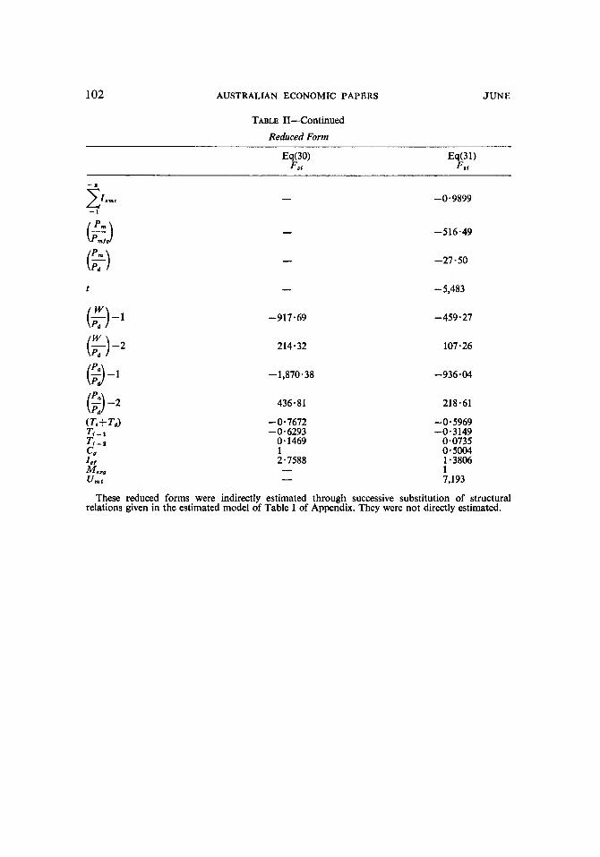
through the production functions and through the investment functions. We use notation Ff for F estimated by (22) and F, for F estimated by (23) when investment was estimated through production functions, and Ffi and FSi respectively when investment was estimated through investment functions. The reduced forms are presented in Table I1 of the Appendix.

Substituting the observed value for the exogenous variables, we can obtain the estimates of the endogenous variables for the sample period. Since the production of services is assumed to depend on the production of the manufacturing and social overhead sector by equation (1 l), in order to generate alternative endogenous values, we have to feed in alternative values only for the production variables of the primary sector and the manufacturing and social overhead sector. For convenience we sub- stituted observed values for primary sector production. Considering the fact that agricultural land in Korea is intensively cultivated, the production of this sector is deemed dependent not so much on capital input as on climatic conditions in the short run.

During the sample period (1957-66), the value added in the manufacturing and social overhead sector grew by an average annual rate of 10.5 per cent. Although the actual rates of growth in individual years differ from 10.5 per cent and accelerated in the latter part of the period, we can substitute the 10.5 per cent for every year and then

TABLE IT F, = foreign exchange gap; F. = savings gap.

Year

Case I Case 2 Growth rate of manufacturing and social overhead sector of 10.5 per cent per year

Growth rate of manufacturing and social overhead sector one per cent higher than

actual rate

Difference between Difference between Constraining gap two gaps as Constraining gap two gaps as

percentage of percentage of smaller gap smaller gap

1957 1958 1959 1960 1961 1962 1963 1964 1965 1966

% 6.1 3.9 5.5

16.5 19.9 9-8 2.5

22.9 79.5 99.4

O /

$3 7 . 6

1 3 . 1 24.9 ~

31.2 9 . 2 6 . 4

34.4 42.7 12.3


estimate the resource gaps as Case 1 in Table 11. Since, on the average, the value added in the manufacturing and social overhead sector together has actually grown by 10.5 per cent, we may deduce that, in any particular year, the gap which was larger acted as the dominant constraint on further growth. It can be seen that, in general, the growth in earlier years was constrained by the foreign-exchange gap while the investment-savings gap was dominant in the latter part of the period.

The comparative size of the two gaps is shown by expressing the difference between them as a percentage of the smaller gap (see column 2 of Case 1). One should not, however, place too much reliance on these estimated differences, as significant errors are not uncommon in all types of macro-estimation. This is particularly true for the estimates of the two gaps derived as residuals according to equations (22) and (23), which contain all the errors that occurred in estimating other endogenous variables. Furthermore, the size of the two gaps is so small compared with the size of other endogenous variables which determine the two gaps, that one can expect relatively larger errors (compared to their true values) for the estimation of the gaps.

Thus it seems fair to ignore those years in which the relative size of the difference between the two gaps was small. The years in which the relative difference was larger than 10 per cent were 1960, 1961 and 1964, when one can see that the foreign-exchange gap was the dominant constraint on growth, and 1965 and 1966, when the investment- savings gap was of greater significance.

Case 2 presents another set of estimates for the two gaps. It is based on the assumption that the manufacturing and social overhead sector grew annually at a rate exceeding the observed growth rate by one per cent in each year, while the primary sector grew at the observed annual rate. Thus we take into account any annual variations in the conditions affecting sectoral growth.

The results in Case 2 are quite similar to those in Case 1 , except for 1962 and 1963 when growth was constrained by the foreign-exchange gap in Case 1 and by the investment-savings gap in Case 2. Again, taking only those years in which the relative difference between the two gaps was higher than 10 per cent, we find that growth in 1960, 1961 and 1964 was constrained by the foreign-exchange gap, and in 1965 and 1966 by the investment-savings gap.

When some supplementary data are examined, however, it is hard to say whether economic growth in 1961 was constrained by the foreign-exchange gap, for there was an increase of 32 per cent in foreign exchange reserves.6 This indicates that actually there was excess foreign exchange in that year. On the other hand, the domestic wholesale price index of imported goods rose by 40 per cent during 1960-61, an indication that imports were in short supply. Politically, both years were highly turbulent, with a student revolt in 1960 and a military coup in 1961. The increase in industrial production was less than in any other year under consideration and there was substantial excess capacity in the manufacturing industries. Putting together these conflicting pieces of evidence, one may conclude that growth in 1961 was not constrained by any resource gap.

In 1965 there was a once-and-for-all devaluation which raised the exchange rate between the United States dollar and the Korean won from the existing 130 won to 255 won. There is a strong indication that foreign exchange was in relatively excess

6Ranis and Fei question also the identifiability of the parameters that were estimated from the historical time series in their comment on the Chenery-Strout disequilibrium adjust- ment thesis in reference to foreian assistance and economic development. See Ranis and Fei, “Foreign Assistance and Economic Development: Comment”, American Economic Review, Vol. 58, 1968.


TABLE 111 Marginal Productivity of Foreign Resource7

Growth rate of Vm,.,% 4 6 8 10

Marginal productivity of external resource 3.420 3.115 2.639 2.029

Growth rate of VmfOv% 11 13 15 17

Marginal productivity of external resource 1.905 1.606 1 *469 1 * 386

supply in 1965 and 1966, and that shortage of investment funds was the dominant constraining factor. The foreign-exchange reserves of the economy increased by 9 million United States dollars and 97 million United States dollars in 1965 and 1966 respectively. In spite of tight credit control in both years, there was an abrupt increase in money supply due to rising foreign-exchange reserves. The increase in money supply was mainly responsible for the rising level of prices in these two years, at a rate of more than 10 per cent per year.

From these results, one can conclude that economic growth was constrained by the investment-savings gap in the latter years and the foreign-exchange gap in the earlier part of the period. The marginal contribution of foreign resources in generating production can be seen from the marginal productivity estimates given in Table 111. Since the average annual rate of growth in value added of the manufacturing and social overhead sector was 10.5 per cent, the marginal productivity would have been approximately two.

Iv. ALTERNATIVE GROWTH PROGRAMMES AND FUTURE mQUIREMENTS

When estimating future requirements, it is necessary to predict values for the exogenous variables. From Table IV below one can see that gap estimates are not very sensitive to moderate changes in variables such as prices, unclassified imports, and stock investment. For convenience, we assume fixed values for these variables, and assume alternative sets of growth rates for the remaining four exogenous variables : tax revenues of the government (Ti+ Td), total exports X , government investment Zg,, and government consumption C,. Alternative rates of growth for exogenous variables,

7 Calculation was done by:

Marginal productivity of external resource = ( ~ V r - ~ V l o . & ) / ( p r - $ F i o . 6)

1 1 1

= sample-period sum of gross national product under r per cent of annual growth in manufacturing and social overhead sector, given observed values for primary production.

= sample-period sum of gross national product under 10.5 per cent of annual growth in manufacturing and social overhead sector, given observed values for primary pro-

= sample-period sum of foreign savings under r per cent of annual growth in manufacturing and social overhead sector, given observed values for primary production.

= sample-period sum of foreign savings under 10.5 per cent of annual growth in manufacturing and social overhead sector, given observed values for primary pro-

$ v1 O. I) duction.

>l O. I) duction.

1972 FOREIGN ASSISTANCE AND KOREA'S ECONOMIC GROWTH 97

which were derived either from the past experience of the economy or the Economic Development Plans of the government, provide different sets of strategies that the economy should follow.

TABLE IV Elasticity Estimates

F, Ff F*, Ff I

12.5348 9.2214 1.1454 0.5998 1 * 7984 4.0335

1.0659 1 4072

0.8666 0.2406 0.8666 1.3527

0.9883 0.9883 0.1953 0.1953

0-5490

0.0290

0.0748

2.3751 0.0800 1.0659 1 *4072

0.6770

0 * 5490

0.0290

0.0748

Table V presents the growth rates of exogenous variables in alternative programmes. The main implications of these strategies for achieving self-sustaining economic growth are also summarized below.

TABLE V Alternative Programmes

(Rate of increase per annum) (Unit : %)

A 5

16 7.8

18 7 1.8

10

B 5

11 7.8

18 7 1.8 7.2

C 5

16 17.3 22.3 10.9 13 10

D 5

11 17.3 22.3 10.9 13 7.2

E F G 5 5 5

20 20 16 30 30 30* 40 30 40** 35 35 35 10 10 10 12 12 10

r,, = rate of growth of the pi ...I ary sectoi I value adL-- r = rate of growth of the manufacturing and social overhead sector's value added Y = rate of growth of the gross national product

* 30% (1967-69); 25% (1970); 20% (1971); 15% in subsequent years ** 40% (1967); 25% (1968-70); 20% (1971) and 15% in subsequent years

A. The rates of growth of exogenous variables were derived from the average of the period of 1957-66, while the rate of growth adopted for the manufacturing and social overhead sector is from the Second Five-Year Plan. Under this programme, self- sustained growth will not, however, be achieved. Until 1970, the investment-savings gap will constrain economic growth; thereafter the import-export gap will be the limiting factor.


B. The assumptions about the exogenous variables are the same as in A. The rate of growth of the manufacturing and social overhead sector is equivalent to the First Five-Year Plan target. The dominant gap is investment-savings until 1973, after which the growth of the economy will be self-sustaining.

C. The rates of growth of the exogenous variables all come from the Second Five- Year Plan, as does the rate of growth of the manufacturing and social overhead sector. In the earlier part of the next ten-year period, self-sustained growth will be attained.

D. The assumptions are the same as those in C except that the rate of growth of the manufacturing and social overhead sector becomes the target rate of the First Five-Year Plan. This is again a very easy programme, self-sustained growth being attained in the latter part of the ten-year period.

E and F. The assumptions for the rates of growth of the exogenous variables as well as that of the manufacturing and social overhead sector were derived from the latest (1965-68) experience of the economy. It seems that these programmes are not feasible, for the ratio of tax to the gross national product would become exorbitant in the latter part of the next ten-year period.

G. This programme is also based on the latest (1965-68) experience of the economy, but more moderate rates of growth were assumed for the export and tax variables. Tax has actually increased by 30 per cent per annum in recent years, while exports have grown by 40 per cent per annum. These rates were also maintained in the year of 1968. However, in future it may be increasingly difficult to maintain these rates of growth. Tax is, therefore, assumed to increase by 30 per cent per annum until 1969, 25 per cent in 1970, and by 15 per cent per annurn in the subsequent period. Exports will grow by 40 per cent in 1967, 25 per cent per annum until 1970 (although they have actually grown by 40 per cent in 1968), 20 per cent in 1971, and then by 15 per cent per annum in the subsequent period.

A stage of self-sustained growth can be attained if this programme is carried out. It should, however, be regarded as an upper-target programme for the next ten-year period, Already there is mounting scepticism about whether the present rate of performance can be maintained.

V. CONCLUSION Korea has been more successful than other recipients of foreign aid in utilizing

foreign resources to accelerate her rate of economic development. The Second Five- year Development Plan assumes that this trend will continue.

We found that it will be essential to maintain the high rates of increase in both tax revenue and exports if gross national product is to grow at the present rate of 10 per cent per annum and if the economy is to achieve a stage of self-sustained growth. However, the recent export performance has been helped significantly by the booming demands of the Vietnamese War, so one could expect increasing difficulties in sustaining such a high rate of growth of exports in the future. In order to reduce the investment-savings gap which is likely to limit the rate of growth of gross national product, the economy will be required to increase significantly its tax efforts in every year.

1972 FOREIGN ASSISTANCE AND KOREA'S ECONOMIC GROWTH

APPENDIX

The model system estimated for the purpose is as follows:

TABLE I A Statistical Model of the Korean Economy

c, =

c, =

I,? =

Mj =

. ~. ,

Ra'= Oa'997 d = 2 .8 - _

1 13,861 So. 767(( v, - 1+ V-,,) -(Ti+ Td))- (9.01) (36.46)

R a = 0.994 d = 1.8

-72,096+0.6294(PD-PD - 1) - 1+0'482PD - a+ 1 ~75881~1 (-12.38) (8.82) (12.37) (11.86)

R a = 0.998 n = 1.7 - - .

60,918+0*2776Cp-567.9 (Q-Q-i)-1,570.7Q-l (4.81) (5.44) (-3.08) ( - 5 -59)

R a = 0.860 d = 2.1

M, = 36,031+0*1645Vm~,.-328~7 -1

(4.51) (8.35) (-4.21) (-2.24) R a = 0.957 d = 2.2

(3.87) (8.05) (-1.66) (-5.03) (-4.16) R a = 0.980 d = 2.6

- 5,477+0*2688Ij+ 7,193 Urn, (-8.02) (38.53) (11.73

I , I .

R P = 0.996 d = 2.7

-6,109+0.0198V-27*5

(-5.40) (8.84) (-1.74) R P = 0.941 d = 2.7

21 3,945 + 1 . 1747Ka- 17,038 Ua (30.19) (13.26) (-3.40)

48,452 + 0.3522 KrnfO. (11.00) (27.63)

157,086+O*3733Km (23.79) (12.53)

R a = 0.970 d = 1.5

R a = 0.990 d = 1.5

R a = 0.952 d = 1.7

141,408 + 0 * 5853 Vmioo (28.69) (19.80)

R a = 0.980 d = 2.0

99

(4)

100 AUSTRALIAN ECONOMIC PAPERS

TABLE I-Continued

Y/ = -290,889+1,672.4Q+2,971.9 - (3 (-23.16) (24.59) (23.98)

R a = 0.996 d = 1.5

(3 Y w = - 130,919+0*4587 Vna+ 1,458.1

(-4.00) (14.34) (6.42) R' = 0.971 d = 2.0

JUNE

(12)

i21i

Notation:

*Endogenous variables * V * V. * Vmlou = gross national product originated in manufacturing and social overhead sector * V, Td+ T,= direct taxes minus netcurrent transfersto theprivate sector plus indirect taxes minussubsidies *C = consumption *CQ = private consumption *I = gross capital formation C,, = government consumption

* I f I , = increase in stock I, Imlou = gross fixed investment in manufacturing and social overhead sector I,,

* I Q f = private fixed investment I,,, = government fixed investment

*M = imports *My = import of food *M, = import of raw materials *Me, = import of intermediate materials *Mt = import of machinery and transport equipment * M a , = private import of service

*Y, = farm income * Y , = labour income *PD = non-farm and non-labour income *F = foreign savings

* V,. *S = gross domestic savings *KO *Kmfo. = cumulative gross fixed investment in manufacturing and social overhead sector since 1953 *K,

Q

= gross national product = gross national product originated in primary sector

= gross national product originated in service sector

= gross fixed capital formation

= gross fixed investment in primary sector

= gross fixed investment in service sector

Me,, = unclassified import of goods plus government import of service

X = exports = gross national product originated in non-primary sector

= cumulative gross fixed investments in primary sector since 1953

= cumulative gross fixed investment in service sector since 1953 = grain production index, 1953 = 100


= ratio of implicit deflator of primary production to the implicit GNP deflator

= ratio of implicit import deflator to implicit deflator of value added of the manufacturing

= ratio of implicit import deflator to implicit deflator of GNP, 1965 = 100

= ratio of per employee monthly earnings index of manufacturing sector to implicit GNP

U. = weather dummy variable, 1 for 1957,1959, 1960,1962, 1963, 1965, and 0 for other years Un,t = dummy variable, 1963 = 1, 1965 = I , and 0 for other years r = time in years

(&) and social overhead sector, 1965 = 100

(k) deflator, 1957 = 100

Ismi= lagged three-year cumulative investment in imported inventory goods - 1

The stochastic equations were estimated by the ordinary least-squares method, and were based on

The figures in brackets below estimated coefficients are “t” ratio adjusted for the degrees of

d is the Durbin-Watson statistic.

the data from the National Income Accounts of Korea, the Bank of Korea, 1967.

freedom.

TABLE I1 Reduced Form

Eq(28) FI

Q Q - I I ,

80.945 --,- - - 4.0385

-4.4075 - 0.1487 -0.0841

1

- -0.7672 1

-14,504 - -

249,245 -0.3690

-0.1261 -1

1 .3965 -0 * 1469

0.5400

- -

- 1,052.55 245.81 1

189,455 2.9709

-2.2057 0.4458

-0.2130 -1 -567.85 - 1,002-80 -

-0.9899

-51 6.50

-27.51

-5,483 -0.2129 - 1 7,259 7,193 273,681

0.7652 0.2702

-0.0631 0.0198 0.5279

-0.0735 -1 -567.85 -1,529.55

123.02 -

102 AUSTRALIAN ECONOMIC PAPERS

TABLE 11-Continued Reduced Form

JUNE

- 5 16.49

-27.50

1 - - 5,483

-911.69 -459.21

214.32 107.26

( 2 - 1 -1,870.38 -936.04

436.81

-0.7672 -0.6293

0.1469 1 2.7588 - -

218.61

-0.5969 -0.3 149

0-0735 0.5004 1.3806 1 7,193

These reduced forms were indirectly estimated through successive substitution of structural relations given in the estimated model of Table I of Appendix. They were not directly estimated.

foreign assistance and korea's economic growth

Documents