Foreclosure Contagion:Measurement and Mechanisms 1

David J. Munroe and Laurence Wilse-SamsonColumbia University

December 14, 2013

1David Munroe: Department of Economics, Columbia University, email address: djm2166@columbia.edu. Laurence Wilse-Samson: Department of Economics, Columbia University, email address: lhw2110@columbia.edu. Financial assistance from the Program for Economic Research at Columbia University andthe Social Sciences and Humanities Research Council of Canada is gratefully acknowledged. We are thankfulto Ethan Kaplan, Wojciech Kopczuk, Suresh Naidu, Doug Almond, Patrick Bolton, Janet Currie, ChrisMayer, Tomasz Piskorski, Bernard Salanié, Joseph Stiglitz, and Miguel Urquiola for comments and advice.We would also like to thank Alicia Horvath at Record Information Services Inc. for assistance with data.

Abstract

In this paper we ask whether foreclosures are contagious: does a completed foreclosure causeneighboring foreclosure filings? We estimate this relationship using administrative data on homeforeclosures and sales in Cook County, IL, and instrument a completed foreclosure using randomassignment of chancery-court judges. We find that a completed foreclosure causes between 0.5 and0.7 additional filings within 0.1 miles, an effect that persists for several years. We interpret our re-sults as evidence that contagion is driven by borrowers (rather than lenders). Moreover, contagionis not driven by borrowers in negative equity, but by borrowers learning from neighboring foreclo-sures. We also find that foreclosure disrupts local housing markets, increasing sales of neighboringlower-quality properties.

1 Introduction

The housing bubble and crisis of the last decade has resulted in an unusually large number offoreclosures in the United States. Completed foreclosures—when a mortgage borrower does notmake payments on their loan and the lending institution claims the mortgaged property—increaseddramatically starting in 2007 from 404,849 properties per year, peaking at 1.05 million completedforeclosures in 2010.1 The length and severity of this crisis has increased academic interest inthe consequences of home foreclosures and have raised questions about how and why foreclosuresspread.

In this paper we ask whether home foreclosures are contagious: does one completed foreclosureincrease the probability that geographically neighboring borrowers end up in the foreclosure pro-cess? The answer to this question informs our understanding of home foreclosures, borrower andlender behavior, and policy toward mortgages and foreclosure procedures. Foreclosure contagion issuspected of exacerbating the housing crises during the Great Depression and the recent financialcrisis (Campbell (2013)). Identifying contagion in foreclosures will provide a better understandingof how and why such crises spread. Furthermore, the presence of contagion is relevant to policymakers concerned with mitigating the spread of home foreclosures.

Our chief contribution is to develop a randomly assigned instrument for foreclosures, which weapply to administrative data to achieve credible, policy-relevant estimates of foreclosure contagion.In Cook County, IL, where foreclosures cases are decided in court, we use the randomizationof new foreclosure cases to fixed groups of judges as an instrument for a completed foreclosure.Intuitively, our estimates compare the neighborhoods around two types of properties going throughthe foreclosure process (i.e., situations in which a borrower is in default and the lender wants toclaim the home as collateral): properties randomly assigned to “difficult” judges that, as a result,end up being foreclosed upon and sold at auction versus properties randomly assigned to “lenient”judges that dismiss the foreclosure case. Since our empirical strategy necessarily relies on thecomparison of neighborhoods around homes in default that do and do not end in foreclosure, ourestimates speak directly to the policy question of how strongly lenders should be incentivized torenegotiate delinquent loans.2

We develop a novel data set that matches administrative records of foreclosure court cases to1We use “foreclosure filing” to refer to the initiation of the foreclosure process by the lender, and “completed

foreclosure” to refer to a foreclosure proceeding ending with the mortgaged property being sold at auction. However,lenders are not always successful in foreclosing on a home, and so not all filings end in completed foreclosure—werefer to such unsuccessful foreclosure attempts as “dismissals.”

2There is a developed literature that uses judicial bias as an instrument, as we do herein, including: Kling (2006)(sentencing propensities of judges to instrument for incarceration length); Autor and Houseman (2010) (job placementrates of non-profit contractors to instrument for receiving temporary help jobs); Chang and Schoar (2006) (judicialfixed effects to measure judge-debtor-friendliness); Dobbie and Song (2013) (judge discharge rates to instrumentfor bankruptcy protection); Doyle (2007) (placement frequency of child protection investigators to instrument forfoster care); French and Song (2011) (allowance frequency of administrative law judges to instrument for receipt ofdisability insurance); Maestas et al. (2013) (allowance rates of disability examiners to instrument disability insurancereceipt); and Aizer and Doyle (2011) (incarceration tendency of randomly-assigned judges to instrument for juvenileincarceration).

1

records on foreclosure filings and auctions for Cook County. This county, which contains most ofthe city of Chicago, is the second-most populous county in the U.S. and was relatively hard hit bythe housing crisis: the surrounding MSA experienced the 12th largest decline in city-wide housingprices between 2007 and 2011, while 5.2% of the 1.9 million households in Cook County experi-enced a completed foreclosure. Our data covers the universe of foreclosure filings and completedforeclosures in Cook County between 2004 and 2011, allowing us to leverage the random assignmentof foreclosure judges while observing the precise location of the associated property. We also useadministrative data on residential housing sales to assess whether a completed home foreclosurelowers neighboring housing values.

Concrete evidence on foreclosure-related externalities and contagion has been elusive, owing toempirical challenges (Frame (2010)). Home foreclosures are known to be correlated with neigh-borhood characteristics and changes in housing prices and macroeconomic circumstances (Mianand Sufi (2009); Mian et al. (2011)). Existing studies that find negative housing price effects offoreclosure have relied primarily on local analyses that explicitly control for property and neighbor-hood characteristics (Campbell et al. (2011), Immergluck and Smith (2006), Schuetz et al. (2008),Pennington-Cross (2006), Leonard and Murdoch (2009), and Lin et al. (2007)) or repeat-sales anal-yses (Harding et al. (2009) and Gerardi et al. (2012)). Similarly, existing studies finding evidenceof foreclosure contagion rely either on local analyses (Towe and Lawley (2013)) or aggregate anal-yses controlling for neighborhood and zip code characteristics (Goodstein and Lee (2010)). Fewstudies have taken a quasi-experimental approach to identifying the externalities associated withforeclosure.3 Ours is the first study to use a randomly assigned instrument to estimate contagionand local price effects of home foreclosures.4

Using our instrumental variables strategy to compare neighborhoods with completed foreclo-sures to neighborhoods where foreclosure cases are dismissed, we find evidence of foreclosure con-tagion. Relative to dismissal of a foreclosure case, a completed foreclosure raises the probabilityof any new foreclosure filing within 0.1 miles by 10% per year and leads to about 0.5 new filingsper year. We find that this foreclosure contagion effect is persistent, lasting for three to four yearsafter the case is decided. Additionally, our estimates show that substantial contagion in foreclosurefilings occurs even in neighborhoods with no recent foreclosures—the “first” completed foreclosurein a neighborhood substantially increases foreclosure filings in the following years. Moreover, ourresults demonstrate that contagion is not limited to new foreclosure filings—we also observe anincrease in neighboring completed foreclosures, suggesting that contagion is costly and plays a role

3One exception is Mian et al. (2012) who exploit changes at state borders in policy toward foreclosure (judicial vs.non-judicial states) to instrument foreclosures, although this instrument is not randomly assigned (for example, Pence(2006) shows substantial changes in housing market conditions at the boundaries between judicial and non-judicialforeclosure states).

4There is a related line of research that focuses on non-pecuniary costs of foreclosure, such as whether foreclosurescause crime (Cui (2010); Goodstein and Lee (2010); Ellen et al. (2013)) or harm health (Currie and Tekin (2011)).Additionally, several existing studies address the question of own-price discounts of home foreclosures. Campbellet al. (2011) find a substantial discount for the sale of foreclosed properties (as well as other types of distressed sales),while Harding et al. (2012) argue that the observed foreclosure discount is a fair price for those properties—investorswho purchase real-estate owned properties are not reaping unusually large profits.

2

in the geographic spread of foreclosures. Lastly, we find that a completed foreclosure influencesthe effort that neighboring borrowers and lenders put into ongoing foreclosure proceedings: a com-pleted foreclosure increases the number of completed foreclosures even among neighboring casesthat began prior to the event.

While we find evidence that a completed foreclosure lowers neighboring residential sale prices,our estimates are largely driven by selection into sale. Within the first year of a case ending in aforeclosure, relative to a case that ends in dismissal, the average price of neighboring housing salesdrops by up to 40%. However, using a repeat-sales methodology to adjust for property quality,our estimates of this effect fall substantially. We interpret this as evidence that a completedforeclosure disrupts the housing market in terms of the types of homes that sell, causing a largershare of lower-quality homes to transact at correspondingly lower prices than the average homein the neighborhood. At the same time, due to the small size of our housing sales sample andthe resulting imprecision of our housing price estimates, we cannot rule out a negative effect ofcompleted foreclosure on neighboring home values (holding quality constant).

We find evidence consistent with the commonly held belief that foreclosure contagion is drivenby an increase in borrowers defaulting on their loans in response to a neighboring foreclosure,rather than lenders filing for foreclosure against already delinquent borrowers. There is substan-tial evidence that lenders and mortgage servicers—third parties employed by creditors to manageloans—indiscriminately favored pursuing foreclosure on delinquent mortgages, rather than modifi-cation (see discussions in Adelino et al. (2009); Foote et al. (2008); Levitin and Twomey (2011)).We argue that in the absence of borrower-driven contagion, lenders would not exhibit positive fore-closure contagion. Given that we do observe positive contagion provides evidence that borrowersrespond. Moreover, we find substantial contagion even among mortgages serviced by lenders knownfor automating foreclosure procedures and who are, thus, unlikely to respond to very local marketconditions.

There are two prominent explanations of why a completed foreclosure will increase the proba-bility that neighbors default on their own mortgages. The first hinges on a completed foreclosurelowering neighboring home values, thus increasing the likelihood that borrowers are “underwater”on their loans—i.e., owing more than the mortgaged property is worth (Campbell and Cocco (2011),Campbell (2013), Goodstein et al. (2011)). As one becomes further underwater on one’s loan, theincentive to default on the mortgage increases: the loss on the asset grows large relative to the costsassociated with foreclosure (primarily moving costs and a drop in credit score). The second expla-nation is that a completed foreclosure transmits information to neighbors (Guiso et al. (2013), Toweand Lawley (2013)). Specifically, a completed foreclosure may send a signal to neighbors aboutthe future of the neighborhood (influencing the expected value of the property to the borrower), orabout the foreclosure process itself (e.g., neighbors may learn about the likelihood of a mortgagemodification if they default on their loans).

We find that contagion is concentrated among borrowers who are not underwater on their mort-gages, which we interpret as evidence that contagion is not driven by foreclosures causing falling

3

housing prices. Using information about housing values, and loan principal and outstanding bal-ance, we construct a proxy for borrowers being underwater. We find that contagion is driven not byborrowers in negative equity (underwater), but by borrowers in positive equity. We expect under-water borrowers to be more sensitive to falling home values than those in positive equity (Campbelland Cocco (2011)), and, thus, interpret this difference in effects as evidence that contagion is notdriven by falling home values. Rather, we expect that foreclosures convey information to neighbors:a neighboring foreclosure may act as a “wakeup call” for borrowers in positive equity, sending astrong signal about the future of the neighborhood and/or information about the foreclosure pro-cess itself, while those who are underwater on their loans may already be well informed about theforeclosure process and the consequences thereof.

We find that contagion varies substantially depending on whether borrowers have mortgagesserviced by the same lender, which we interpret as further evidence that information plays animportant role in driving contagion. Specifically, we find that when a completed foreclosure occursthere are significantly fewer new foreclosure filings among loans serviced by the same lender thanloans serviced by different lenders. This difference may be driven by borrowers learning moreand different information from the experience of neighbors whose loans are serviced by the sameinstitutions: how long the foreclosure process takes, how actively the lender pursues foreclosure,and the probability of a loan modification.

Our results suggest that policies that keep delinquent borrowers in their homes, for example byencouraging lenders to modify delinquent loans, may reduce the spillovers associated with homeforeclosures. We are able to speak to this question since our empirical strategy identifies foreclosurespillovers for the set of marginally delinquent loans for whom the idiosyncrasies of the overseeingjudge matter (i.e., the cases that are likely to comply with the instrument)—these are the casesmost likely to be influenced by policy interventions. In principle, our results provide support forgovernment policies that encourage modification, such as the Treasury’s Home Affordable Modi-fication Program (HAMP) (even if there have been considerable (and well documented) problemsin implementation). Of course any program must weigh general equilibrium considerations—theseinclude the effects on ex-ante incentives for loan origination, and incentives for default by otherborrowers. Our finding that contagion is minimal or even negative among borrowers with the samecreditors, may provide evidence that these incentives for strategic default matter—we interpret thisfinding as demonstrating that borrowers update the probability of a modification downward andare discouraged from defaulting on their loans. As such, a policy that raises the cost of default(e.g., achieving a reduction in loan principal only by going through bankruptcy, as suggested byLevitin (2009)) or a more direct policy that targets the vacancy and neglect associated with REOproperties may be preferred.

The rest of the paper proceeds as follows: In Section 2 we outline the judicial foreclosure processin the state of Illinois and randomization of judges to cases in Cook County. Section 3 sketches ourdata sources—administrative records on court cases, geocoded administrative records on foreclosurefilings, and deed transfer records. In Section 4 we outline the empirical strategy, which exploits the

4

random assignment of judges for quasi-experimental identification, the results of which we presentin Section 5. Section 6 explores possible mechanisms, and Section 7 concludes.

2 Judicial Foreclosure in Illinois

Cook County, Illinois, provides a good context in which to study foreclosure contagion. Firstly, itwas badly affected by the foreclosure crisis. Between 2002 and 2011, the county saw 302,166 fore-closure proceedings initiated by lenders (“foreclosure filings”), and 134,924 completed foreclosures.These trends are illustrated in Figure 1. The upper panel of the Figure shows a sharp increase inthe number of foreclosure cases filed in Cook County from about 1000 per month in 2004 to morethan 3000 filings per month in 2008. The lower panel demonstrate that foreclosure proceedingsbecame more likely to end in a completed foreclosure: the completed foreclosure rate jumps from45% for cases filed in 2004 to 65% in 2008. Secondly, the foreclosure process in Cook County,IL, goes through the court system, allowing us to instrument a foreclosure outcome using randomassignment of judges to cases.

In Illinois, as in many so-called “judicial foreclosure” states, lenders must take delinquent bor-rowers to court in order to claim a mortgaged property. When a borrower has missed three mortgagepayments (i.e., is in default), a lender or the third party servicing the mortgage may initiate theforeclosure process by filing for foreclosure on the associated property with the chancery court (werefer to this event as a foreclosure filing). If after ninety days the borrower has not made up allmissed payments, the trial begins and the lender’s attorney must establish that the borrower: hasborrowed money from the lender; has signed a mortgage note promising the property as collateral;and is behind on payments. At the same time, the borrower may mount a defense, for exampleby disputing any of these facts or claiming that the lender has violated lending laws (e.g., theTruth-in-Lending Act). After hearing the arguments, the presiding judge decides the case, eitherdismissing the foreclosure action or filing a judgment of foreclosure. If the case is dismissed, theborrower typically continues to reside in the home. If a judgment of foreclosure is filed, then thecase proceeds to a foreclosure auction, which we refer to as a completed foreclosure.5 If the saleprice does not cover the outstanding balance of the mortgage then the borrower is still consideredin debt to the lender, although it is common for lenders to forgive this remaining debt. In the vastmajority of cases (around 95% for Cook County), the lending institution purchases the property atauction for the amount of the outstanding loan—in doing so the lender need not record a loss ontheir balance sheet.6

A dismissal may refer to several possible outcomes, most of which result in the property remain-5When a foreclosure judgement is made, a redemption period begins during which the borrower may pay off the

entire outstanding mortgage (not just missed payments) plus late fees, attorney fees, court costs, and taxes. Theredemption period ends either three months after the judgment or seven months after the initial foreclosure complaintis served, whichever is later.

6See statistics for Cook County compiled by the Woodstock Institute:blog.cookcountyil.gov/economicdevelopment/wp-content/uploads/2012/11/Wodstock-Institute-Foreclosure-Filings-2007-2012.pdf

5

ing occupied by the borrower. First, if a borrower makes all missed payments within 90-days of thefiling, then the case is dismissed and the mortgage is reinstated. Second, rather than continuingto pursue an ongoing foreclosure case, the lender may modify the terms of the mortgage to makepayments more affordable to the borrower. Third, a lender may accept a deed-in-lieu of foreclosure,in which the borrower forfeits the home to the lender without going through the courts. Fourth, theborrower may negotiate a short sale of their home: the lender accepts the proceeds from the sale ofthe home as payment for the mortgage. Deed-in-lieu of foreclosure and short sales are generally notan option when there are multiple liens on the property, a fact we exploit to confirm that our resultsare not driven by these outcomes in which delinquent borrowers lose their property (Agarwal et al.(2011)).7 Fifth, the lender may “lose” the case by failing to adequately establish non-payment ofthe mortgage or that they are owed the debt, or the borrower’s defense may be successful. Finally,a case may be dismissed because the lender does not take action in pursuing the foreclosure. In ourdata we cannot distinguish which of these outcomes occurs; we only know whether the case endsin dismissal or completed foreclosure. However, with the exception of a deed-in-lieu of foreclosureor a short sale, in all of these dismissal outcomes the house remains occupied by the borrower.

Foreclosure cases (as with all chancery court cases) are randomly assigned to a case calendar,which restricts the set of judges that will ever hear an action on the case. A case calendar is a weeklyschedule of court-room/judge pairings, usually made up of two or three judges. Judges typicallyonly hear cases associated with their case calendar. Similarly, since chancery court cases are onlyassigned to one calendar, only the associated judges will oversee an action on that case. Whena case is filed, it is assigned a unique case number, sorted by property type (single-family home,condominium, commercial property, etc.), and randomly assigned to a case calendar.8 As of 2010,there were 12 chancery court case calendars hearing foreclosure cases (there are additional calendarsthat hear only other chancery court cases). Judges are assigned to case calendars each year by theChief Judge of the Circuit Court of Cook County (details of these assignments are outlined in theGeneral Administrative Orders of the court available online at www.cookcountycourt.org/).9

There are several ways that a Cook County judge might influence the outcome of a foreclosurecase, which is necessary for the validity of our instrument.10 Firstly, the judge has discretion to

7Anecdotally, deed-in-lieu of foreclosure and short sales are uncommon in Cook County for the reason that, inboth cases, creditors are typically taking a loss, while mortgage servicers will accrue lower fees (relevant in caseswhere the property is being managed by a mortgage servicer): in Illinois, by accepting a deed-in-lieu of foreclosurethe lender must forgive all debt, while short sales typically transact at a price below the outstanding debt (Ghentand Kudlyak (2011)).

8Random assignment of cases to case calendars is performed by the Chancery Court computer system. As describedon the Chancery Court’s FAQ page “When a case is filed in the Law Division it is randomly assigned via a computerprogram to a calendar letter. You may contact the Information Desk in Law Division to obtain the Judge’s informationassociated with the calendar letter.” See www.cookcountyclerkofcourt.org/?section=FAQSPage

9Not all calendars hear foreclosure cases in equal proportion. For example, throughout our sample (2004–2011)three of the calendars (Chancery Court calendars #52, #53, and #54) hear both foreclosure cases and other chancerycases, while others hear exclusively foreclosure cases. Thus, while assignment is random, the probability of assignmentto a given calendar is not uniform.

10There is substantial evidence of so-called judicial bias in many settings: Anderson et al. (1999) illustrate im-portant differences across judges in decision-making—sometimes suggestive of some forms of bias (see for example,Abrams et al. (2008) or Yang (2012)), and sometimes more generally based on “personal assessments” of case-specific

6

determine how long a defendant has to find a lawyer and mount a defense. Secondly, even if adefendant does not mount a defense, the judge determines whether or not the lender successfullyestablishes that the borrower is behind on payments and that the debt is owed to the lender.Establishing these points is less trivial than it seems. Throughout the foreclosure crisis, there havebeen accounts of mistakes and wrongdoing in the prosecution of foreclosures, including wrongfulforeclosures on current mortgages, and failures of banks to produce proper documentation, lendersinitiating foreclosure proceedings without reviewing the history of the loan (“robosigning”), failuresto adequately attempt to renegotiate the terms of the loan or follow government policy aroundmodifications (c.f., Kiel (2012)). Similarly, it us up to the judge to evaluate a borrower’s defense,for example by determining whether a mortgage is legal in the first place (e.g., is not in violationof (predatory) lending laws). Anecdotal evidence suggests that judges vary substantially in theirleniency on these issues.11In our analysis of Cook County court records we find substantial variationby judge in the rate of completed foreclosure.

In what follows, we use the random assignment of foreclosure cases to case calendars to instru-ment the outcome that the case ends in foreclosure. As discussed above, judges may influence theoutcome of a case. At the same time, the case calendar to which a foreclosure case is randomlyassigned determines the possible judges who will ever hear the case. If judges vary sufficiently intheir biases toward foreclosure, then the case calendar to which a case is assigned may influencewhether a case ends in foreclosure or dismissal. Thus, our identification relies on the comparisonof two delinquent borrowers going through the foreclosure process, one of whom is randomly as-signed to a “lenient” case calendar and ends in dismissal, while the other is randomly assignedto a “strict” calendar and ends in foreclosure. To implement this study we require data on CookCounty foreclosure cases, including case calendar assignment and the case outcome (foreclosure ordismissal).

3 Data

We use geocoded administrative data for Cook County from three sources: Cook County chancerycourt records, foreclosure filings, and deed transfer records. Publicly available chancery courtrecords for 2004–2010 provide us with details of each foreclosure case, including the informationnecessary to construct our instrument: the case calendar to which the case is randomly assignedand the outcome of the case (dismissal or foreclosure). To study neighborhood outcomes, however,we need to know the location of the borrowers’ homes. To this end, we match each chancerycourt foreclosure case record to the associated foreclosure filing record (2002–2011), which has beeninformation (Iaryczower (2009)). Berdejo and Chen (2010), for example, present evidence suggestive of unconsciousjudicial bias—illustrating priming effects on judges of wars (which suppress dissents)—as well as more partisanbehavior before Presidential elections.

11The Washington Post observes, for example, that “[in] Suffolk and Nassau counties on Long Island and KingsCounty... which have among the highest rates of foreclosure in the state and where the 81 judges handling foreclosureshave become infamous over the past few years for scrutinizing paperwork ... the level of tolerance for documentmistakes varies from judge to judge ...” (emphasis added). “Some judges chastise banks over foreclosure paperwork”,Washington Post, 9 November 2010.

7

provided to us by Chicago-based Record Information Services, Inc. (RIS). These records allow usto observe new foreclosure filings that occur around any given delinquent homeowner’s property,which we use to study foreclosure contagion. To observe how completed foreclosures affect housingmarkets—prices and sales volumes—we rely on deed transfer records (1995–2008) provided to usby the Paul Milstein Center for Real Estate at the Columbia Graduate School of Business. Theserecords allow us to observe the state of the housing market around each property going through theforeclosure courts. Finally, we bolster the information about each neighborhood using data fromthe 2000 Decennial Census, Zillow housing price indices, and IRS Statistics of Income.

The Cook County chancery court makes public all court records, which include details oneach foreclosure case. We manually collected data for each of the 217,230 chancery court casesfiled between January 1 2004 and June 30 2010 from the court’s public electronic docket.12 Eachrecord identifies the case number (a unique identifier assigned by the court), the type of case(e.g., foreclosure vs. other chancery case), the plaintiff (lending institution or mortgage servicer),the defendant, and the case calendar. The records also include every action on the case (andcorresponding date), although the action descriptions offer minimal detail.

We rely on foreclosure filings from RIS to identify the location of properties going through theforeclosure process. The RIS data span all 307,209 foreclosure cases filed between 2002 and 2011in Cook County (although some records are for properties in neighboring counties). These recordscontain the same variables as the online chancery court records, except RIS does not collect thecase calendar. However, RIS also collects information not included in the court records, such as thetype of property (single-family, condo, etc.), details about the mortgage (type of mortgage, originalloan principal, outstanding balance at time of foreclosure filing), and any additional lien holdersidentified on the filing.13The RIS data provide us with the address and latitude/longitude of thehome under foreclosure. Finally, RIS also collects a record of each foreclosure auction between 2002and 2011 (168,577 in total). This allows us to conclusively observe a foreclosure outcome and thedate that the foreclosed property is sold.

We match the chancery court records to the RIS foreclosure filings by case id.14 The resultingdata set covers 174,187 foreclosure filings in Cook County filed between January 2004 and June2010. For our analysis, we drop 847 filings associated with Veterans Affairs mortgages (VA), 12,755filings made during the Cook County foreclosure moratorium of 2009,15 and 12,365 filings madeduring the first or last year in which a case calendar hears foreclosure cases, as cases may be non-randomly assigned as the calendar makes the transition.16 Ultimately, our results are not sensitive

12www.cookcountyclerkofcourt.org13The lender’s attorney is not required to identify additional lien holders.14See the Data Appendix for more details on the cleaning process.15Cook County enacted a moratorium on new foreclosure filings on April 16, 2009 to last through September 1,

2009. This moratorium applied to all new filings except those in which the borrower agreed not to mount a defenseprior to filing. The effect of the foreclosure moratorium can be seen in Figure 1: in the upper panel, we see that thenumber of cases filed dips sharply during the moratorium. Interestingly, it seems as though the moratorium finishedearly—there is a spike in new filings before September 1, 2009. In the lower panel, we see a jump in the completedforeclosure rate for cases filed during the moratorium.

16Case calendars have been added over time to ease the burden on existing calendars. In our data, we observe the

8

to these sample restrictions, although the inclusion of filings on “new” case calendars brings our IVestimates closer in line with the OLS estimates, suggesting some non-random assignment to newlyintroduced calendars.

This matched data allow us to observe key dates and outcomes of foreclosure cases. For eachrecord, we observe the date the case is filed, and whether and when the case is dismissed orforeclosed, the location of the home under foreclosure, and the above-mentioned details of theproperty and mortgage. We consider a case as ending in completed foreclosure if the RIS recordsindicate that a foreclosure auction occurs for that property and mortgage, and we consider theauction date to be the end of the case. We consider a foreclosure case as being dismissed if itdoes not have an associated foreclosure auction and if the chancery court data records a dismissalaction, where we take the date of the dismissal action as the relevant “dismissal date” (see the DataAppendix for details of these variable definitions).

The majority of cases end in a completed foreclosure, while a small fraction of cases are unre-solved due to right-censoring of our data. As can be seen in Table 1, which provides descriptivestatistics (imposing the above-mentioned sample restrictions), 90,653 (61.2%) cases have an associ-ated foreclosure auction, 50,140 end in dismissal (33.8%), and the remaining 7,427 foreclosure casesremain undecided due to right-censoring. The average length of a case is about 373.6 days, althoughthis is significantly longer for cases that end in foreclosure (428.7 days vs. 274.9 for dismissals).Since the Cook County chancery court records are up to date as of the date of collection (early2012), and the RIS foreclosure auctions are up to date through 2011, we do not observe the end ofparticularly long cases. This is especially true for cases filed in 2009 and 2010, from which 79.08%of the undecided cases originate. We omit these undecided cases from our analyses (as well as casesfor which we observe the decision, but do not have data on our outcomes for that year).

Among dismissals, we see that only 12.0% of the borrowers “redefault”, suggesting that thedismissal outcome does not merely delay a completed foreclosure. We define redefault as a newforeclosure filing occurring against the same loan after the first case has been decided. Note thatthis definition of redefault is specific to a given loan and does not count future defaults to the sameborrower on different loans and future defaults from different borrowers at the same property. Sincedismissed cases make up our counterfactual in studying the neighborhood-level effects of completedforeclosures, this low rate of redefault is reassuring—in most instances dismissing a case does notmerely delay the foreclosure (for example, while the lender finds a missing mortgage note), butprovides a concrete resolution of the mortgage default within the time frame that we observe.17

To study the neighborhood-level effect of completed foreclosure on housing sales and prices we

addition of six new calendars to the foreclosure roster and the phase-out of 16 calendars (that move from hearingforeclosure cases to hearing exclusively other chancery cases). Unfortunately, the details of these phase-in and phase-out processes are not well publicized and we observe unusually low case assignment to these calendars during thephase-in periods. Our concern is that as new calendars are introduced to the foreclosure process they are restrictedin the type of foreclosure cases that they hear.

17Notice that there is also a non-zero number of redefaults (1.3%) among loans that end in foreclosure. This islikely due to miscoding in the RIS data—for example, a foreclosure auction is scheduled and recorded by RIS, thecase is dismissed before the auction takes place (and RIS misses this) and the borrower subsequently redefaults onthe loan. Our results are not sensitive to discarding these observations.

9

rely on deed transfer records for Cook County from 1995–2008. These records cover the universeof real estate transactions and indicate the date of sale, the sale price, and the property type(residential, commercial, etc.). We restrict this data to residential real estate transactions between2000 and 2008,18 which leaves us with 862,215 residential real estate sales. The mean sale price forthese transactions is $276,401, while the median is $215,000. We geocode the transactions usingthe reported property address (using Yahoo! Placefinder), allowing us to observe transactions nearproperties associated with foreclosure cases.

Finally, we add data from the 2000 Decennial Census, the IRS Statistics of Income (SOI), andZillow. We match these data sources to the Cook County chancery court cases by census tract(Decennial Census) and zip code (IRS SOI and Zillow). The Census provides us with details (asof 2000) on the population density and race of the census tract in which each property is located.The IRS Statistics of Income provide a measure of zip-code-level income (mean adjusted grossincome) derived from aggregated tax returns. These data are available for the 1998, 2001, 2002,and 2004–2008 tax years (for 2003, we use the mean of 2002 and 2004, while for 2009+ we usethe observed adjusted gross income in 2008). Finally, Zillow provides zip-code-level housing priceindices for 2000–2011.

4 Empirical Strategy

Our primary objective is to estimate whether and to what extent a completed home foreclosure iscontagious, which we define in terms of the question: does one completed foreclosure cause newforeclosure filings? To this end, we compare the number of new foreclosure filings in neighborhoodsaround properties going through the foreclosure process that end in a completed foreclosure toproperties that end in dismissal. An obvious concern is that there is non-random selection intocompleted foreclosure (versus dismissal); we deal with this endogeneity and omitted variable bias byinstrumenting a completed foreclosure using the random assignment of foreclosure cases to chancerycourt case calendars.

For each property that goes through the foreclosure courts, we measure all outcomes annuallywithin an x-mile radius of the property. We measure outcomes relative to the date that the case isdecided (either the date of the foreclosure auction or the date of the court action in which the caseis dismissed). For case i, let d(i) be the time period in which the case is decided and Yi,d(i)+t bethe outcome for property i measured within an x-mile radius of the property, t periods from thedecision date. In practice, we measure time in terms of years: d(i) is the year in which case i isdecided, d(i) + 1 is the year after the case is decided, and so on.19 In our baseline specification weuse a 0.1-mile radius around each property, although our results are not sensitive to taking smalleror larger radii (of the same order of magnitude). As an example of how we construct our outcomes,one measure of contagion we consider is the number of new foreclosure filings within a 0.1-mile

18See the Data Appendix for more details.19We have also tried months and quarters. However, since home sales and foreclosure filings in small geographic

areas are low-frequency events, estimates using these finer units of time end up being low-powered and imprecise.

10

radius of each property every year since the case is decided.To achieve our goal of comparing cases filed at the same time that have different outcomes

(owing to the random assignment of case calendars) we include several sets of fixed effects in ourbaseline specification. Filing-month fixed effects, Mm(i), where m(i) is the filing month associatedwith case i, allow us to compare foreclosure and dismissal among cases filed at roughly the same time(and, as explained below, we construct our instrument at the filing-month level). However, casesfiled in the same month may be decided in different years. Since we do not want our estimatesto be based on the comparison of cases decided in drastically different times (e.g., the onset ofthe financial crisis in 2008 versus the peak of the boom in 2006) we include year-of-observationfixed effects, ψd(i)+t.20 In our baseline specification, we also include property-type fixed effects, Φi

(single-family home, condo, etc.), as cases are sorted by property type prior to randomization tocase calendar. Finally, we include a vector of covariates, Xi (loan principal at origination, a dummyvariable for the lender/plaintiff being a “large” plaintiff (six largest plaintiffs each representing ≥7000 filings), a dummy variable for the plaintiff having a “large” attorney (three largest attorneyseach representing ≥10,000 cases), whether the census tract has an above-median share of whiteresidents, a set of dummy variables for the quartile of median census-tract income, and censustract population density). While these controls improve precision, our estimates are robust toexcluding both the property-type fixed effects and the covariates. The resulting relationship weestimate is:

Yi,d(i)+t = β0 + β1Fi + βXi + Mm(i) + Φi + ψd(i)+t + ui,d(i)+t (1)

where Fi is an indicator for case i ending in foreclosure. Our goal is to estimate β1 from Specification1 separately for each value of t ∈ {0, 1, 2, 3, 4, 5} for contagion and t ∈ {0, 1, 2} for price and saleseffects (due to data limitations).

We cluster our standard errors along two dimensions: filing month and census tract (Cameronet al. (2011)). Clustering on filing month captures correlation due to macroeconomic trends—cases filed in the same month may experience similar shocks. Since we also expect correlationbetween properties that exist in the same geographic area, we cluster at the census tract level.One issue with multi-way clustering that we occasionally encounter is invalid negative varianceterms (and a non-positive-definite variance matrix). As suggested in Cameron et al. (2011), weconservatively address this by taking the maximum of the standard errors clustered only on filingmonth, clustered only on census tract, and clustered on filing month and census tract (and theminimum of the corresponding first-stage F-statistics).

20One concern is that the length of the case is itself endogenous. We have explored this in several ways: in TableA.1 of the appendix we add controls for the length of the case and find that our contagion results hold. In Table A.2we estimate the baseline effects measuring the outcome as of the date that the foreclosure case is filed (rather thandecided). While this measurement leads to somewhat noisier estimates (the treatment is diluted by cases that havenot yet been decided) the results are generally consistent with our baseline contagion estimates.

11

4.1 Measuring Local Contagion and Prices

We define two outcomes to test for contagion. Firstly, we consider an indicator for whether anynew foreclosure filing occurs within x miles of property i in year d(i) + t—how does a completedforeclosure affect the probability of observing any new foreclosure filing? Secondly, we consider thecount of new foreclosure filings within x miles of property i in year d(i) + t—how does a completedforeclosure affect the total number of new filings? In both cases, we omit new foreclosure filingsat the same address or associated with the same foreclosure case but at a different address (e.g.,a loan taken with multiple properties as collateral). We also consider the effect of a completedforeclosure on the probability of any and total number of neighboring completed foreclosures.

We also examine the effect of a completed foreclosure on local housing prices, although hereour estimates are hampered by sample size. Our measure of local housing prices for the propertyassociated with case i is constructed by taking the log of the average sale price of all properties thatsell within the x-mile radius of property i in the year of observation d(i) + t. Importantly, we omitthe delinquent property itself to ensure that our price estimates are not influenced by an own-pricediscount of foreclosure (as found by Campbell et al. (2011)). One concern with this measure isthat it does not account for selection into sale—the types of homes that sell after a completedforeclosure may be different from the types of homes that sell after a dismissal, and this selectionmay drive any observed price effects. Unfortunately, we do not observe any proxies for propertyquality in our data.

We take two approaches to addressing bias from selection into sale. Firstly, while we cannotestimate selection in terms of the types of homes that sell, we can observe whether the volumeof sales itself changes. For each property going through the foreclosure process, i, we take asan outcome the count of sales that occur within x miles of property i in the year of observationd(i)+ t (again omitting sales at the delinquent property itself). A change in the quantity of sales inresponse to a completed foreclosure suggest that some sellers (or buyers) are selecting into or outof the market. At the same time, observing no significant response of quantity of sales does notprove that price effects are not driven by selection, but is reassuring—the influx of low (or high)quality properties would have to offset the drop in high (or low) quality properties.

Secondly, we study the subset of repeat-sales (about 44% of the sample) in our data in order toadjust for fixed property characteristics. We estimate the quality-adjusted home value by nettingout property-specific fixed effects—details of this adjustment procedure are in the appendix. Ourestimates of the effect of a completed foreclosure on the log of the mean quality-adjusted pricewill not be biased by selection into sales under two assumptions. Firstly, we assume that thereis not differential occurrence of repeat sales around properties that end in completed foreclosurevs. dismissal. Since this analysis is restricted only to repeat sales, if this assumption is violatedwe will have selection into the sample. Secondly, we assume that the property characteristics thatdetermine sale price are not changing differentially for properties near a completed foreclosure vs.a dismissal (i.e., the error in the repeat-sales adjustment process is invariant to the case outcome).Even if these two assumptions hold, our repeat-sales estimates may suffer from imprecision due to

12

measurement error in the repeat-sales adjusted measure of home value.Comparing the means of the various outcomes, as displayed in Table 2, shows suggestive evidence

of foreclosure contagion and a foreclosure price effect. These averages are constructed using allconcluded cases (with the above-mentioned sample restrictions) observed annually for five yearsafter the case decision for contagion outcomes, and two years after for price and sales. Specifically,each observation represents a case-year (so a case that is observed for three years after the decisionwill appear three times). The means in the upper panel of Table 2 suggest foreclosure contagion.Properties associated with cases that are dismissed see 0.435 fewer new foreclosure filings per yearthan properties associated with foreclosures. There is also evidence that completed foreclosuresdisrupt the housing market. Properties that end in foreclosure tend to see a higher volume ofneighboring sales (3.099 per year relative to 2.962 near dismissed homes). At the same time, thesesales occur at a lower average price—$157,181.90 vs. $184,212.50—although this difference is notapparent in the repeat-sales-adjusted price. While these descriptive statistics suggest negativeexternalities of home foreclosure, these comparisons of means suffer from omitted variable bias andendogeneity of home foreclosure.

4.2 Instrumental Variables Approach and First Stage Regression

There are several reasons home foreclosures may be endogenous to neighborhood-level characteris-tics. A completed foreclosure is not a random event—it is the product of the choice of a borrowerto default on a loan, the choice of a lender to pursue a foreclosure, and the actions of the associatedattorneys and judges. The borrower default decision may be influenced by local housing prices, thetype of mortgage a borrower has, and the borrower’s financial position (both in terms of balancesheet, and cash flow). For example, foreclosures may be more likely to occur in neighborhoodswith lower housing price levels and negative price growth (Campbell and Cocco (2011)). Similarly,the lender’s decision to pursue a foreclosure versus a loan modification depends on the home value,the probability that the borrower re-defaults on a modified loan, the probability that the borrowerbrings him/herself out of delinquency without a modification, and, if the loan is serviced by acompany that is not the creditor, the potential fees associated with foreclosure (Foote et al. (2008),Levitin and Twomey (2011)).

Descriptive empirical evidence suggests that observable borrower and neighborhood character-istics are correlated with home foreclosures. Table 1 shows means for various covariates brokendown by case outcome, where the fourth column contains the p-value on the test of equality be-tween the foreclosure and dismissal. Cases that end in foreclosure are significantly less likely tosingle-family homes (59.0% vs. 68.4%), more likely to have a plaintiff that is a “large institution”(47.3% vs. 47.2%) or have a plaintiff represented by a “large attorney” (68.7% vs. 68.2%), are lesslikely to have a conventional fixed-rate mortgage (65.3% vs. 66.5%), and tend to be in neighbor-hoods with lower median income (43,748.26 vs. 46,409.49), a lower share of white residents (43.3%vs. 46.8%), and a lower population density. While studies have attempted to control for omittedvariable bias using very local fixed effects analyses (see summaries in Foote et al. (2009), Towe and

13

Lawley (2013)), ours is the first study to directly address the endogeneity of home foreclosure witha randomly assigned instrument.

We use a measure of the propensity to foreclose for each chancery court case calendar as aninstrument for completed foreclosure. We construct our instrumental variable to capture the notionof judicial bias—the judges on some case calendars are more likely to foreclose than others, all elseequal—by taking the “jackknife” or “leave-one-out” foreclosure rate for each case calendar, as iscommon in studies that use judicial random assignment as an instrumental variable (e.g., Kling(2006), Doyle (2007), Dobbie and Song (2013)). Specifically, for each case i, filed in month m(i)and randomly assigned to calendar k, we take the foreclosure rate among all other cases j filed inthat month and assigned to that calendar:

Zi =�

j∈Km(i),j �=i Fj

n(Km(i)) − 1 (2)

where Km(i) is the set of all cases filed in month m(i) and assigned to calendar k, n(Km(i)) is thecardinality of set Km(i), and Fj = 1 if case j ends in a completed foreclosure.

A case calendar with “strict” judges whose cases end often in foreclosure will have a high valueof the instrument, Zi, while a calendar with “lenient” judges will have a low value. By omittingcase i when constructing the instrument, we ensure that we are not regressing the outcome of thecase on itself (resulting in a mechanical correlation in the first stage). Calculating this instrumentat the filing-month level accommodates changing case-calendar rosters and attitudes of judges overtime.21 Failing to account for these changes may violate monotonicity of the instrument.

Our first-stage regression relates an indicator for a case ending in foreclosure to our measure ofcase-calendar strictness. For each case, we regress an indicator for the case ending in foreclosure(Fi) on the instrument. As with the second stage described in Specification 1, we include filingmonth fixed effects, Mm(i), property-type fixed effects, Φi and year of observation fixed effects(Ψd(i)+t). One concern is that judge attitudes may respond to macroeconomic events, includingthe foreclosure boom, and the financial crisis. At the same time, the types of borrowers who aredefaulting on their loans is likely also changing over time (Mian and Sufi (2009)). This concern isaddressed by the inclusion of the filing month fixed effects. The resulting first-stage regression is:

Fi = α0 + α1Zi + αXi + Mm(i) + Φi + Ψd(i)+t + vi (3)

We rely on the usual instrumental variables assumptions: the instrument influences the outcomeof the foreclosure case (instrument relevance), the instrument is randomly assigned (instrumentexogeneity), the instrument does not itself influence neighborhood outcomes (exclusion restriction),and an increase in the instrument is associated with an increase in the probability of the case endingin foreclosure (monotonicity). Table 3 presents OLS estimates of Specification 3 (omitting year ofobservation fixed effects, as these are only relevant in the full 2SLS procedure). Column 1 shows

21For example, we see in Figure 1 that the foreclosure rate changes over time.

14

a strong relationship between the case calendar foreclosure rate and the probability that a caseends in foreclosure—a one percentage-point increase in the case-calendar foreclosure rate increasesthe probability of a completed foreclosure by 0.556 percentage points (or about 0.91% off themean foreclosure rate of 0.612). Including the case-specific covariates does not appreciably changethis relationship. Moreover, this relationship is strong—the first-stage F statistic of the excludedinstrument is 150. Thus, the assumption of instrument relevance seems valid.

We test exogeneity of the instrument by looking for systematic correlation between the instru-ment and pre-filing case characteristics. If the rules of the Chancery Court are followed, then theinstrument should be randomly assigned and appear independent of case characteristics. We runtwo sets of regressions to check the assumption that the instrument, Zi, is randomly assigned. First,we regress Zi on a set of pre-treatment covariates (controlling for property type and filing month):

Zi = γ0 + γXi + Mm(i) + Φi + ei (4)

where Zi is the instrument, Xi is a vector of fixed or pre-treatment property and case characteristics,and Mm(i) and Φi are filing month and property type fixed effects. Random assignment impliesthat none of the covariates predict the value of the instrument (H0 : γi = 0) and that the covariatesdo not jointly determine the value of the instrument (H0 : γ1 = γ2 = ... = γk = 0). Second, weregress each of these covariates on a full vector of case calendar dummy variables (again controllingfor property type and filing month):

Xji = ρ0 +�

k

ρkκki + Mm(i) + Φi + ui (5)

where Xji is a given pre-treatment characteristic j observed for case i, and κki is a vector ofcalendar-specific dummy variables such that κki = 1 if case i is assigned to calendar k. We thentest the joint significance of these dummy variables: H0 : ρ1 = ρ2 = ... = ρk = 0 .

We present the results from these randomization-check regressions in Table 4. The first columnpresents the coefficient estimates from Specification 4 and the p-value for the joint significance testof the covariates. We see no evidence of systematic correlation between pre-treatment covariatesand the instrument, and cannot reject the hypothesis that the covariates are jointly insignificant.The second column displays the p-value for the joint significance test of case calendar dummiesfor Specification 5, where the outcome variable is given by the row. Again, there is no systematicrelationship between case calendar assignment and pre-treatment covariates, with the exception ofloan principal. We conclude that, conditional on filing month and property type, case calendarsare randomly assigned.

The assumption that the instrument does not itself influence neighborhood-level outcomes isreasonable. The outcomes we are studying are the result of the decisions of those not involvedin the court case (e.g., neighboring home owners). Moreover, while foreclosure cases span manymonths, defendants will have minimal direct contact with the presiding judges.

Finally, we find no evidence of a failure of monotonicity. The assumption maintains that a

15

higher value of the instrument—i.e., being assigned to a stricter case calendar—weakly increasesthe probability of foreclosure for all cases. One can imagine, however, a prejudiced judge whomay be lenient toward delinquent wealthy borrowers, for example, but push for foreclosure againstdelinquent borrowers of lower social class. Then if there are disproportionately more of one typeof borrower, a higher value of the instrument will not mean a higher probability of foreclosure forall cases. We explore this possibility by relating group-level foreclosure rates (e.g., foreclosure rateamong cases in predominantly white vs. non-white census tracts) within each case calendar tothe overall foreclosure rate for each calendar and find that foreclosure rates for sub-groups are allincreasing with the overall case calendar foreclosure rate. A discussion of these results can be foundin the appendix.22

4.3 Interpretation of the Two-Stage Least Squares Estimate

Our estimate captures the LATE for foreclosure cases in which judges are influential, compounds theeffect of all subsequent completed foreclosures caused by the initial foreclosure, and is representativeof neighborhoods with many foreclosure filings. The estimate does not represent the effect of acompleted foreclosure relative to a mortgage that is in good standing; rather, the estimate representsthe effect of a completed foreclosure relative to the effect of a foreclosure case being dismissed. Weargue that this parameter is of central interest to policy makers.

Firstly, as discussed in Doyle (2007), if there are heterogeneous treatment effects the parameteridentified by a judicial random assignment instrumental variable (or in Doyle’s case, rotationallyassigned case workers) is the LATE for “marginal” cases—those where the judge is likely to havean influence. Intuitively, there are cases that will always end in foreclosure and cases that willalways end in dismissal; the set of “compliers” with our instrument are the marginal cases wherethe judges on the case calendar have influence on the outcome.23

We find that the characteristics of the sub-population of loans that comply with our instrumentare consistent with cases on the margin of foreclosure or dismissal, representing individuals who havea higher ability to pay than the typical delinquent borrower, but are facing difficult circumstancesthat could be mitigated through loan modification. We stratify the sample along several margins:tract-level quartile of income (from the 2000 Decennial Census), whether the loan is from a “large”lender, whether the mortgage is conventional, whether the zip code experiences positive price growthin the year that the case is filed, and a proxy for whether the property is worth less than the loan

22As suggested by Mueller-Smith (2013), we have also estimated our baseline specification by constructing theinstrument separately for various sub-groups. If monotonicity is violated, then these results may differ substantiallyfrom the baseline estimates. While we do not see a substantial difference in our baseline results (see Table A.3 in theAppendix), these “monotonicity-robust” estimates are imprecise; constructing the group-specific instrument placeshigh demands on the data, as splitting the data into filing-month/characteristics cells often yields few observationsper cell.

23It is easy to conceive of situations where judges will not matter. For example, some sophisticated or well-to-doborrowers may always be able to renegotiate the terms of their mortgages (and a dismissal of the case), regardless ofwho the judge is. At the same time, other borrowers may resign themselves to walking away from their home andmortgage and choose not to appear in court at all (with a foreclosure as a result).

16

(“underwater”).24 Our goal is to proxy characteristics of borrowers who are likely to benefit fromloan modification; creditors may be more willing to modify in such situations (Adelino et al. (2009)),making them more responsive to judicial input.

We estimate the first-stage relationship for each subgroup and compare the estimate of theparameter on the instrument (judicial leniency) to the estimate of the same parameter for the fullsample. Specifically, for each sub-sample, G, we estimate the first-stage:

Fi = α0 + α1GZi + αXi + Mm(i) + Φi + Ψd(i)+t + vi ∀i ∈ G (6)

We then take the ratio of the estimate of the first-stage relationship for group G to the estimate forthe full sample from Specification 3: ˆα1G

α1. As described by Angrist and Pischke (2008), the ratio

of the sub-group-specific first stage to the full-sample first stage represents the relative likelihoodthat a complier belongs to the given subgroup.

We interpret our estimates of these ratios, presented in Table 5, as demonstrating that compliantcases are likely to be on the margin of completed foreclosure. The upper panel, which displaysestimates for the four quartiles of tract-level income, show that compliers are more likely to be inthe upper two quartiles of income than the general population of foreclosure cases. Taking incomeas a measure of a borrower’s ability to repay their loan, these estimates suggest that compliers aremore likely than the typical borrower to be able to resume payments if the case is dismissed.

At the same time, the compliant sub-population may benefit from a mortgage modification.Compliant borrowers are less likely to be in a zip code with positive price growth. Falling houseprices may be largely responsible for the default crisis (Mayer et al. (forthcoming))—borrowers maybe in default because they expect to lose money on their mortgages as housing prices fall and thevalue of the asset drops below the cost of the debt. A modification reducing either the principal ofthe loan or the interest rate may reduce the loss anticipated by the borrower making default (andforeclosure) less appealing. At the same time, compliant borrowers are not in dire straits—theyare less likely to be underwater on their loans, so a modification may be more effective (homevalue is not so low that the mortgage is a lost cause) and may result in smaller losses to lendersthan modification of more severely underwater loans. Additionally, compliers are less likely to haveconventional loans. There is some suspicion that unconventional mortgages are responsible formany defaults during the crisis. For example, borrowers with low “teaser” interest rates or balloonpayments may have been expecting to refinance their loans to avoid higher monthly payments, butfound themselves without this option during the financial crisis. In such cases, a modification maybe particularly effective (by mimicking the effect of a refinance).25 Finally, it is interesting to notethat the differential characteristics of the compliant population appear borrower specific—compliers

24We define a proxy for a borrower being underwater by relating the initial loan size to the outstanding debt whenthe foreclosure case is filed. We start with the initial loan principal, assume an 80% loan-to-value ratio at origination,and back out an estimate of the initial home value. We then adjust this value using zip-code-level housing priceindices from Zillow to arrive at an estimate of the value of the home at the time of foreclosure. We deem the borrowerto be substantially underwater if the lender’s claim against the borrower is greater the estimated home value.

25At the same time, there is debate about the importance of unconventional loans in the default decision (c.f.,Mayer et al. (forthcoming)), so this channel may be less relevant.

17

are no more or less likely to have a loan from a “large” lender.Secondly, our LATE estimate does not simply identify the effect of a single completed fore-

closure, but compounds the effects of all subsequent induced foreclosures. If foreclosures are con-tagious, then a completed foreclosure will lead to subsequent foreclosure filings. Naturally, someof these filings will, in turn, become completed foreclosures and themselves cause new foreclosurefilings. Since our empirical strategy compares the local neighborhoods around cases in the foreclo-sure courts each year after the case is decided and does not control for the effects of subsequentforeclosures, our estimates will compound the effects of these subsequent foreclosures. We believethat this parameter is policy-relevant since it represents the overall consequences of the marginalforeclosure—given a delinquent borrower, what are the external costs of a completed foreclosurerelative to a dismissal of the case?

Similarly, if there is foreclosure contagion, our LATE represent neighborhoods with several com-pleted foreclosures. Recall that our unit of observation is the neighborhood around a property goingthrough the foreclosure courts. This represents a selected sample—we only observe a neighborhoodwhen a foreclosure filing is pursued against a property. Moreover, if completed foreclosures inducesubsequent foreclosure filings resulting in additional observations in our data, neighborhoods withcompleted foreclosures will be over-represented in our sample. This does not affect the validity ofthe instrument—case calendars are still randomly assigned—but influences the interpretation ofthe LATE.

Finally, our estimates are conditional upon a foreclosure filing having occurred in the neighbor-hood. Our empirical strategy and data set necessarily rely on comparing neighborhoods aroundproperties that are already going through the foreclosure process. Our estimates will not accountfor any externalities associated with a borrower default or a foreclosure filing. Many have arguedthat it is a completed foreclosure and subsequent real-estate ownership of the associated propertythat drives foreclosure-related externalities. While we cannot speak to any spillovers from borrowerdefault, our estimates provide a well-identified answer to whether there are negative spillovers asso-ciated with the completed foreclosure itself. To date, existing estimates of foreclosure externalitieshave confounded these two channels.

The LATE represented by our estimates is a relevant parameter for the policy question of howbest to address the problems of delinquent borrowers. Policymakers concerned with foreclosures canfocus on several stages of the lending process: how easy it is to originate/obtain mortgages, how toprevent borrowers from defaulting, and what to do once a borrower has defaulted. Our parameter,which is estimated conditional on foreclosure filing, focuses directly on the latter question.26 Forexample, if we find large negative externalities of a completed foreclosure relative to a dismissed case,then policymakers may want to consider incentivising lenders to renegotiate delinquent mortgages.Moreover, the LATE is relevant for cases on the margin of foreclosure and dismissal, and whoare influenced by foreclosure court judges. These cases are also likely to be influenced by policies

26Of course, the usual partial-equilibrium caveat applies: any change to foreclosure policy may affect ex-anteincentives (e.g., Mayer et al. (2011)) and housing market outcomes (e.g., Pence (2006)), which are not captured inour reduced-form estimates.

18

discouraging foreclosure on delinquent loans.A number of existing government policies to address the foreclosure crisis focused on incentiviz-

ing servicers to perform home mortgage modifications. These include the FDIC’s Loan ModificationProgram, “Mod in a Box”; the GSE variant of this, “the Streamlined Modification Program,” andmost significantly the Treasury program—Home Affordable Modification Program (HAMP). Whilethere have been important criticisms around implementation, our estimates help to address thequestion of whether these are sensible programs in principle.27

5 Neighborhood-Level Effects of Completed Foreclosure

We find robust evidence of foreclosure contagion that persists over several years. Neighborhoodsaround a completed foreclosure are 10% more likely to have at least one foreclosure filing in agiven year relative to neighborhoods around a dismissed property and experience around 0.5 to 0.7more total filings per year. We also find that residential properties that transact around completedforeclosures do so at a price discount (on the order of 30–40%), although this effect may be largelyexplained by negative selection into sale.

5.1 Contagion in Foreclosure Filings

Our estimates demonstrate that completed foreclosures are contagious. Table 6 presents our base-line 2SLS estimates of the effect of a completed foreclosure on the probability of observing anyneighboring foreclosure filing in a year and on the annual count of neighboring foreclosure filingswithin 0.1 miles of the at-risk property. The 2SLS estimates show that a completed foreclosureincreases the probability of observing any new filing within 0.1 miles by 0.052 percentage points inthe year of the decision (a 7.4% increase in the mean for all dismissed cases). This effect increasesover time to 8.2 percentage points (11.7%) in the second year after the decision, 9.0 percentagepoints (12.8%) in the third, and 24.7 percentage points (35%) in the fourth year out. Similarly,the 2SLS estimates show that a completed foreclosure causes 0.54 to 0.70 new foreclosure filingsper year in the year the case is decided and the following three years. This contagion representsa 25–32% increase in total annual filings relative to an average of 2.161 filings per year arounddismissed properties. Note that the instrument is strong in the year of the decision through thesecond year after the decision (F-stats around 200), although is relatively weak three, four and fiveyears out owing to the smaller sample for these periods.

Our contagion estimates are generally not sensitive to the specification, sample, or geographicmeasurement of the outcome. The results are robust to excluding the covariates, omitting theproperty fixed effects, dropping cases decided in the summer months (the court automaticallydismisses inactive cases during this time), using a monotonicity-robust instrumental variable, usingthe full sample and including the foreclosure moratorium, omitting each filing year one by one,

27Criticisms have centered around the incentives for servicers to perform these modifications and the lack of principalreduction in the modification plans.

19

dropping neighborhood-years with foreclosure filings above the 99th percentile, and restricting thesample to cases for which we observe at least three years post decision (see Tables A.3, A.4, A.5,and A.6 in the Appendix). This last specification is of particular interest, since it maintains aconstant sample across observation-years, and demonstrates that the evolution of contagion overtime is not driven by changes in the composition of the sample. We also estimate our baselineresults measuring outcomes within 0.25 miles of the delinquent property and find that contagion(and price effects, discussed below) persist—See Table A.7. Note, however, that the estimatesfor price and any foreclosure filing are generally smaller (effects decline as we are further fromthe property), while the effects for total filings tend to be larger (as the radius goes the total basenumber of properties to file for foreclosure grows). Finally, we confirm that our estimates are drivenby dismissals where the defendant retains possession of the property (rather than deeds-in-lieu offoreclosure or short sales). We estimate our baseline results on the sample of cases in which theplaintiff identifies that there are additional liens against the property. Although less precise, thepoint-estimates for this sample are comparable to the full-sample estimates and are not significantlydifferent (see Table A.8 in the Appendix).

We further explore the validity of our estimates by applying the same 2SLS procedure to ourcontagion outcomes measured in the three years prior to the case being filed. If our instrumentalvariable is truly randomly assigned, we should not expect to see any effect of a case ending inforeclosure before the case has even started. We present these “pre-treatment” estimates in Table7. Reassuringly, when instrumented by case calendar leniency, a case ending in foreclosure appearsto have no relationship to local housing prices prior to the start of the case—the point estimatesare close to zero and insignificant.

We examine the cumulative effect of a completed foreclosure in order to appreciate the full extentof contagion. Rather than using as an outcome the number of new foreclosure filings per year foreach year since the decision, we instead consider the total number of new filings since the decision.These estimates are presented in the lower panel of Table 6 and show that a completed foreclosureleads to a significant divergence in foreclosure filings relative to a dismissal. As noted above, inthe year of the decision a completed foreclosure causes 0.691 new filings. However, neighborhoodsaround completed foreclosures have experienced 2.09 more foreclosure filings by the second yearafter the decision, and 6.45 more filings by the fourth year after the case ends. One completedforeclosure may have a substantial impact on the composition of a neighborhood, at least in theshort and medium term.

One concern with our findings is that they are specific to neighborhoods that are experiencinga wave of foreclosures. Firstly, our period of study (2004–2011) is largely made up of the housingcrisis—the Cook County housing market peaked in 2006. Secondly, since we only observe neighbor-hoods where a foreclosure filing has occurred, and since we do find that foreclosures are contagious,there is likely selection into our sample—foreclosure filings (and, thus, observations in our data) arelikely to be in neighborhoods with recent completed foreclosures. From a policy perspective, it isespecially important to understand the cumulative impact of the first foreclosure in a neighborhood.

20

Nevertheless, we find that a completed foreclosure is contagious even in a neighborhood thathas not experienced a foreclosure in recent years. We restrict our sample to cases where there havebeen no completed foreclosures in the two years prior to the decision (the results are similar ifwe restrict to cases with no filings within two years) and estimate the cumulative contagion effectof a completed foreclosure, presented at the bottom of the lower panel of Table 6. We find clearevidence that completed foreclosures are contagious even in neighborhoods with no other recentcompleted foreclosures, although these results are less precise than when we use the full sample,owing to a smaller sample size: a completed foreclosure leads to 1.3 more filings by the end ofthe first year after the decision, and almost four more filings by the third year out. Even the firstcompleted foreclosure in a neighborhood has externalities (and that the contagion we observe isnot an artifact of selection into the sample).28

5.2 Contagion in Completed Foreclosures

To better understand the costs of foreclosure contagion, we look for contagion in completed foreclo-sures. Above, we established contagion in foreclosure filings—the result of new borrower defaultsand lenders pursuing foreclosure action (we take up the discussion of these two actions in moredepth in Section 6). However, if we do not see contagion in completed foreclosures, then contagionin filings is unlikely to be a large contributor to the spread of a foreclosure crisis. Moreover, thecosts of new filings that end in dismissal are, perhaps, smaller than the costs of new completedforeclosures (for example, owing to pecuniary externalities of completed foreclosure, moving costsassociated with the displacement of homeowners, etc.).29

We find contagion in completed foreclosures. We estimate the baseline contagion IV regressionsreplacing the outcomes with an indicator for any neighboring completed foreclosure (within 0.1miles of the property in the given year since the case is decided) and the count of completed fore-closures. We present these estimates in Table 8 and find that a completed foreclosure moderatelyincreases the probability of observing any neighboring completed foreclosure (by 13.8 percentagepoints three-years out). Moreover, there is a notable increase in the number of neighboring com-pleted foreclosures: one completed foreclosure causes between 0.28 and 0.56 additional completed

28Another concern relates to the length of cases—as seen in Table 1, cases ending in dismissal are significantlyshorter than cases ending in completed foreclosure. A possible explanation is that foreclosure externalities are drivenby borrower behavior while in default, and the effect is larger for cases ending in completed foreclosure since thesecases are longer. To rule out this explanation, we estimate our baseline 2SLS estimates, adding flexible controls forthe length of the case. We try three different sets of controls—log of the number of months, a quadratic in numberof months, and dummy variables for the number of quarters of length—and present these results in Table A.1 inthe Appendix. These estimates show contagion effects that are comparable to our baseline estimates, although theaddition of these length-of-case controls reduces the precision of the estimates.

29One difficulty in studying contagion in completed foreclosures is that the response may be driven by judges.While this is not an issue when studying contagion in foreclosure filings—an event that depends only on the actionsof the borrower and lender—judges have an influence over the outcome of a foreclosure case. We cannot explicitlyrule out judge behavior as driving contagion in completed foreclosures. However, we do not expect judge contagion tobe a dominant force—this would require judges to be well informed about recent events in the neighborhoods aroundthe delinquent properties associated with their cases, which we find unlikely given the volume of cases (it would becostly to keep up on all outcomes) and judicial random assignment (judges are not specializing in neighborhoods).

21

foreclosures annually (or between 40 and 93 percent off of the mean). Thus, contagion appears toplay an important role in the spread of foreclosures; mitigating completed foreclosures may reducethe depth and costs of a housing crisis.

The timing of contagion in completed foreclosures suggests that borrowers and/or lenders whoare already involved in the foreclosure process respond to nearby events. Given how long theforeclosure process takes—from default to filing to completed court case—it may seem strange thatwe find contagion in completed foreclosures in the year of the decision. However, borrowers andlenders may respond at any stage of the foreclosure process. For example, a neighboring completedforeclosure may influence the effort a borrower puts into fighting an ongoing foreclosure case byconveying information about the costs of fighting foreclosure or the probability of a successful loanmodification.

Indeed, we find that completed foreclosures influence cases that are ongoing. For each case, i,we split neighboring completed foreclosures into two groups: completed foreclosures among casesfiled before case i is decided and cases filed after case i is decided. By focusing on the formergroup, we can observe how the outcome of case i influences ongoing foreclosure cases. We defineas an outcome the count of completed foreclosures among cases filed before the decision (andan indicator for any completed foreclosure in this group as another outcome) and estimate ourcontagion model—the results are presented in the lower panel of Table 8. The estimates show thata completed foreclosure causes 0.11 to 0.6 new completed foreclosures per year among cases thatwere already filed before the decision in the first two years after the decision (these cases drive thecontagion in the first two years, during which there is minimal contagion among newly filed cases).These results provide evidence that contagion acts not only through influencing the behavior ofborrowers and lenders before filing (e.g., encouraging borrower default), but also by changing howborrowers/lenders approach an ongoing foreclosure case. In particular, it appears that borrowersmay put less effort into resisting a completed foreclosure.

5.3 Housing Markets

Our two-stage-least-squares estimates demonstrate that a completed foreclosure disrupts local hous-ing markets by inducing lower-quality properties to sell, resulting in a lower average sale price. Wefind that a completed foreclosure causes a drop in the average neighboring sale price (not adjustedfor property quality or characteristics) of up to 41% in the following year. However, we find evi-dence suggesting that this drop in price is driven by an increase in sales of lower quality properties.We observe an increase in the number of neighboring sales in response to a completed foreclosure.Moreover, when we use repeat-sales to control for property characteristics, we find no evidence ofan effect of completed foreclosure on average sale prices, suggesting that the unadjusted effect isdriven by selection. Nonetheless, we cannot rule out a small negative effect on quality-adjustedproperty values.

Our baseline 2SLS estimates, presented in the first panel of Table 9, suggest that a completedforeclosure lowers the average neighboring sale price over several years. The columns of Table 9

22

present the baseline price and sales effects for the year in which the case is decided, and one and twoyears after. The estimates suggest that a completed foreclosure depresses neighboring residentialsale prices (by 12.7% in the year of the foreclosure, 41.1% in the year after and 35.8% two yearsout). However, the precision of these estimates suffers from a smaller sample size than our contagionresults (we only observe housing sales through June 2008 and only observe prices when a homesells): they are only significant in the year after the decision and the first-stage F-statistics arerelatively low (around 20). Nonetheless, these estimates are not sensitive to the same robustnesschecks described in Section 5.1 (see Tables A.9, A.4, and A.11 in the appendix). Similarly, we seeno pre-filing relationship between local housing markets and the eventual outcomes of the cases(see Table 7).

Our 2SLS estimates show suggestive evidence that a completed foreclosure influences the volumeof residential housing transactions in a neighborhood. The point estimates of the effect of foreclosureon the probability of any sale are small and insignificant. On the other hand, the point estimates ofthe effect of a completed foreclosure on the cumulative number of neighboring residential sales sincethe case decision shows a large increasing trend—while this effect is not statistically significant, itappears as though a completed foreclosure may induce additional home sales. It may be the case,for example, that a foreclosure signals a future decline in the quality of the neighborhood (or sendsa signal about the local economy), inducing homeowners. This increase in number of sales raises thequestion of whether the drop in sale price after a completed foreclosure is caused by selection intosale of lower quality (and thus, lower price) homes or a drop in the value of neighboring properties(conditional on quality). In particular, if this drive to sell in response to a completed foreclosure isstronger among those with lower-quality houses (for example, because they have less equity in theirhomes or are in a more precarious financial situation), then we would expect a decline in averageneighboring sale price.

Our repeat-sales-adjusted price results suggest that there is negative selection into residentialsales after a completed foreclosure, which may explain much of the negative sale-price effect asso-ciated with completed foreclosure. As explained in Section 3, we use a repeat-sales methodologyto adjust reported sale prices for property quality. We then estimate the effect of a completedforeclosure on the log of the average neighboring quality-adjusted sale price. The point estimatesof the effect of home foreclosure on the log of the mean repeat-sales adjusted price tend to besmall: 0.059 in the year of the decision, 0.003 the following year, and are not significantly differ-ent from zero—controlling for property quality yields smaller price effects of completed foreclo-sure.30 By pooling the unadjusted (i.e., baseline) and repeat-sales-adjusted price regressions andtesting the cross-equation restriction that the effects of completed foreclosure are different (i.e.,H0 : βraw prices = βrepeat sales), we find that the treatment effects for adjusted prices are significantly

30In Table A.10 in the appendix, we confirm that the difference between the baseline and repeat-sales adjustedestimates is not driven by a selected sample of repeat sales. We estimate the baseline price effects for two measuresof neighboring unadjusted price: mean log sale price for all non-repeat sales, and mean log (unadjusted) sale price forall repeat sales. In both cases, the point estimates are comparable to the baseline price effects—large and negative—although the smaller sample size reduces precision.

23

smaller than for the unadjusted prices, although we cannot reject the hypothesis that the estimatesare the same in the year of the decision or two-years out (p-values for this test are presented in theadjusted-price panel of Table 9).

We conclude that there is negative selection into sale—when a neighboring foreclosure occurs,the properties that do sell tend to be of a lower quality. The difference between our repeat-saleadjusted and unadjusted baseline sale price estimates, along with the earlier estimates that suggestan increase in sales volume after a completed foreclosure, suggest that lower-quality homes aremore likely to transact after a completed foreclosure. This may be the case if owners of lowerquality homes in a neighborhood are those who have lower income or wealth. Given a signal thatthe neighborhood is declining (i.e., a neighboring completed foreclosure), these owners may beeager to sell before the neighborhood “falls apart” in order to avoid the liquidity shock, both fromthe difficulty of selling an underwater property and the inability to borrow against an underwaterhome. Of course, we cannot conclude that all foreclosure-related pecuniary externalities are drivenby this selection into sale. Existing studies of foreclosure-price externalities (e.g., Campbell et al.(2011)) find estimates one order of magnitude smaller than our own, and given the imprecision ofour estimates, we cannot rule out that there are negative effects of completed foreclosure on thequality-adjusted value of neighboring properties.

6 Evidence of Contagion Mechanisms

While our reduced-form estimates provide clear evidence of contagion, interpreting the causes ofcontagion is difficult since a foreclosure filing is the result of a joint decision of the borrower,who defaults on his/her loan, and a lender or servicer, that chooses to pursue foreclosure on theborrower’s home. Both parties may be influenced by a neighboring completed foreclosure, whichmay lower the value of the asset and alter the incentives for the borrower to repay and the lender tofile for foreclosure. We argue that by studying heterogeneity in the treatment effect of foreclosures—across loan types, lender identity, and market conditions—we can gain insight into the importanceof borrower and lender behavior.

6.1 Distinguishing Borrower and Lender Response

Our goal is to distinguish whether contagion is driven by borrowers or by lenders. We argue thatlenders would exhibit no response to a local completed foreclosure or even anti-contagion—fewerforeclosure filings in response to a completed foreclosure. This provides a weak test for the presenceof borrower-driven contagion. We then explicitly test for borrower-driven contagion by examiningcontagion among loans from lenders known for automation of foreclosure proceedings (who are,thus, unlikely to respond to very local market conditions).

Lenders and mortgage servicers—third parties who are paid by creditors to collect mortgagepayments and manage defaults—have three options when dealing with a delinquent borrower: donothing, pursue foreclosure, or renegotiate the loan. The action lenders or servicers choose to take

24

influences the observed number of foreclosure filings. Through foreclosure lenders acquire the mort-gaged property and gain the benefit of the value of the property (servicers collect fees for managingthe foreclosure). Lenders or servicers may instead modify the terms of a mortgage with the goal ofmaking the payments more affordable—e.g., a lender might reduce the principal or interest rate ona loan in order to lower monthly payments. The benefit of modification to the lender is ensuringthat a loan continues to be paid, at the cost of a lower lifetime value of repayment. Finally, whenfaced with a borrower who is not making payments, a lender or servicer can always do nothing,although this is generally not optimal.31 Existing empirical studies have found that mortgage mod-ification is uncommon (Adelino et al. (2009), Ding et al. (2009)). There are several (non-exclusive)explanations for why lenders and servicers prefer foreclosure to modification: borrowers may stillredefault on a modified loan (Adelino et al. (2009)); lenders must modify infrequently in order todiscourage strategic defaults among borrowers who can pay, but would like better terms on theirloan (Foote et al. (2008)); foreclosing and purchasing the property at auction allows creditors todelay recognizing a loss on their balance sheets; modification requires coordination and agreementamong all creditors (e.g., multiple holders of a mortgage-backed security or a second lien on theproperty), some of whom may need to accept a loss (Gelpern and Levitin (2009)).

These incentives to file for foreclosure against delinquent borrowers are unlikely to respond toneighboring completed foreclosures (unless borrowers themselves change their behavior), makinglender-driven contagion unlikely. In the Appendix, we adapt the simple framework of Foote et al.(2008) and Adelino et al. (2009) to explore how the lender’s incentive to modify or foreclose mightchange with a neighboring completed foreclosure. Intuitively, assuming that a completed foreclosuredoes not influence the behavior of neighboring borrowers (i.e., no borrower-driven contagion), butlowers neighboring home values, a lender would be weakly less inclined to foreclose on this homesince the collateral is worth less relative to the value of the modified loan (although the lendermay still foreclose for the reasons discussed in the preceding paragraph).32 Moreover, mortgageservicers are not likely to respond to a neighboring foreclosure at all. Servicer compensation inforeclosure depends on fees incurred during the foreclosure process and not on the value of thehome itself—servicers are indifferent to the value of the collateral. At the same time, since servicercompensation on a loan in good standing is typically a function of the monthly payments collected,modifying a mortgage typically entails lower future payments to the servicer and servicers do nottypically recover fees for modifying a loan. Thus, when faced with a delinquent loan, pursuing

31In fact, there are two situations where inaction may be a good strategy. Firstly, if renegotiation and foreclosureare costly to the lender and if there is a high probability that the default will “self cure”—i.e., the borrower willresume making payments—then waiting may be beneficial. Secondly, accounting rules adopted in April 2009 allowcreditors to keep a delinquent loan at face value on balance sheets if there is a reasonable chance that the loan may berepaid. Note, however, that if there is no borrower-driven contagion (i.e., borrowers do not change their probability ofdefault in response to a neighboring foreclosure), then a neighboring completed foreclosure that lowers housing valueswill likely exacerbate these incentives to wait: foreclosures will be even less appealing as the associated property willyield a lower payoff.

32If a completed foreclosure has no influence on neighboring home prices and if we maintain the assumption thatborrowers are unresponsive to a completed foreclosure, then lenders and servicers should not respond—the conditionsof the neighboring loans are unchanged.

25

foreclosure is typically more valuable to servicers, and the decision to take this action is orthogonalto the value of the property. This is consistent with the discussion of Levitin and Twomey (2011)who note that servicers have no stake in the value of the property under consideration, and will takethe action that maximizes the fees they collect, which is typically foreclosure.33 In summary, underthe assumption that borrowers do not respond to completed foreclosures, a neighboring completedhome foreclosure should (weakly) discourage foreclosure filings—the collateral is less valuable tothe lender and servicers are indifferent the home value.

The above-outlined servicer and lender incentives provide a simple test for the hypothesis of noborrower-driven contagion, which we reject. Specifically, this null hypothesis can be rejected ifwe observe positive contagion.

That we observe contagion in Table 6 suggests that borrowers respond. Note, that while thisconfirms the presence of borrower contagion, this does not rule out lender response—when borrowerdefault probabilities are changing, lender response is ambiguous.

To further establish that contagion is driven primarily by borrowers, we study contagion amongloans held by lenders and servicers who are known to have automated foreclosure filing processes.We identify foreclosure filings by all lenders/servicers investigated in the Independent ForeclosureReview Settlement conducted by the Office of the Comptroller of the Currency and the Board ofGovernors of the Federal Reserve System.34 We then redefine our contagion outcomes in terms ofnew foreclosure filings among automating lenders only and re-estimate our baseline 2SLS contagionmodels. The new outcomes are: the count of new foreclosure filings among automating lenders andan indicator for any new foreclosure filing from these lenders. Because this restriction reduces ourpower—we are studying filings among a subset of lenders, which are lower frequency events—wepool all post-decision years (d(i) + t where t ∈ {0, 1, 2, 3, 4}) and restrict the contagion effect tobe constant across all years (see Table A.12 in the Appendix for annual estimates). If contagionis driven largely through lender response, then we should find no effect of a completed homeforeclosure on the number of foreclosure filings among automated lenders. At the same time, ifcontagion is driven primarily through borrower response, then our estimates should be comparableto our baseline full-sample contagion estimates.

33Levitin and Twomey (2011) also point out that, although foreclosure is preferable to modification from theservicer’s perspective, there is incentive to delay the start of the foreclosure process. When a borrower misses apayment, the servicer must forward payment to the creditor as an interest free loan that is repaid to the servicerwhen the borrower resumes payment or the property is sold at foreclosure auction. At the same time, the servicercan charge late fees that are paid when payments resume or the foreclosure sale occurs. Levitin and Twomey (2011)show how servicers can benefit by waiting several months to accrue late fees before beginning the foreclosure process.Of course, this wait period is unlikely to be influenced by a neighboring completed foreclosure, and so does not relateto contagion.

34Throughout the mid- and late-2000s, many lenders and servicers adopted automated foreclosure filing procedures(Levitin and Twomey (2011)). It is clear that in many cases the delinquent borrower’s situation and backgroundwere not given close consideration. As investigations have revealed, employees of several mortgage servicers andfinancial institutions falsely testified that they had personally inspected mortgage borrowers’ information, even thoughthe processing speeds given personnel constraints made it impossible for this to be true (this was the so-called“robosigning” controversy, settled for $25bn in April 2012 between the federal government, 49 state attorneys generaland the five largest servicers). See Kiel, P. “The Great American Foreclosure Story: The Struggle for Justice and aPlace to Call Home”, ProPublica, 10 April 2012.

26

We find that contagion is primarily borrower-driven—contagion in foreclosure filings persistswhen studying loans among automating lenders. Table 10 presents the pooled estimates for allfilings (upper panel) and for filings among automating lenders. One concern is that the totalnumber of loans in a neighborhood from automating lenders is necessarily smaller than the totalamong all lenders (as in the baseline estimates). If new filings are proportional to the existingnumber of loans, then we would expect a larger response in the total count of new filings for thebaseline than for automating lenders. Indeed, this can be seen in column 2: we see a point estimateof 0.74 for the baseline (all filings) and a smaller estimate of 0.115 for the automating lenders.However, relative to the mean number of filings for each group (2.44 filings per year within a0.1 mile radius for all filings, 0.37 for automating lenders), these point estimates are remarkablysimilar: a 30.3% increase in filings versus a 29.7% increase in filings. To further check this concern,we estimate the pooled models using as the outcome the log of the count of new filings. Here, wecan see that the contagion effects are quite similar (0.094 versus 0.084). We also observe similarcontagion in the probability of observing any new filing (0.062 versus 0.039). Thus, given theincentives of lenders and servicers, that the baseline estimates are inconsistent with the hypothesisof no borrower response, and the finding that contagion persists among automating lenders, weconclude that contagion is mainly borrower driven.

6.2 Borrower Incentives

To explore the mechanisms driving borrower contagion, we consider existing theoretical and surveyresearch on borrower default and compare these predictions to estimates with our data and empiricalstrategy. Existing theory of optimal default suggests that borrowers will be more likely to default inresponse to a drop in the value of their home, especially when aggregate housing price growth is low.On the other hand, survey research suggests that learning about foreclosure through social networksmay play an important role in the default decision. We look for evidence of these mechanisms byexamining heterogeneity in the response to a neighboring completed foreclosure. We do not findthat foreclosure contagion is stronger among those in negative equity—with home values below theiroutstanding mortgage debt—but is driven primarily by those in positive equity, which we interpretas evidence that contagion is driven through informational channels rather than a pure housingprice effect. While we cannot conclude that the extent of foreclosure contagion varies systematicallywith social/demographic factors that proxy the strength of social ties in a neighborhood, we dofind evidence of social contagion through a very specific network—neighbors with loans from thesame lender.

6.2.1 Drop in Value of Home

It is commonly held that foreclosures are contagious because they lower neighboring property values(Campbell (2013)). Mortgage default theory (c.f., Campbell and Cocco (2011); Deng et al. (2000))suggests that borrowers are more likely to default when the value of their home falls below thebalance of their mortgage (putting the borrower “underwater”). Intuitively, if the market value

27

of the home is greater than the outstanding debt, homeowners who are having difficulty makingmortgage payments may sell the property and use the proceeds to pay off the debt. Conversely,underwater borrowers who are having difficulty making payments do not have the option to sell.Indeed, descriptive empirical work by Bajari et al. (2008) shows that aggregate housing price declineis one of the most important determinants of mortgage default. To the extent that foreclosures lowercurrent and future neighboring home values foreclosure contagion may operate through pushingborrowers (further) underwater.35

We investigate whether foreclosure contagion is stronger among loans held by individuals whoface high debt relative to the value of their home, as these individuals are likely most sensitive tofalling home values (Campbell and Cocco (2011)). For each foreclosure filing, we create a proxyfor the borrower being underwater at the time of filing. We then split the count of new foreclosurefilings each year within 0.1 miles of each property into two groups: new filings among those whoare underwater and new filings among those who are not. We estimate our baseline 2SLS contagioneffects separately for each type of filing and test the hypothesis that there is more contagion amongunderwater borrowers than borrowers in positive equity.

We define a proxy for a borrower being underwater by relating the initial loan principal tothe outstanding debt when the foreclosure case is filed. We start with the initial loan principal,assume an 80% loan-to-value ratio at origination, and back out an estimate of the initial homevalue. We then adjust this value using zip-code-level housing price indices from Zillow to arriveat an estimate of the value of the home at the time of foreclosure. We deem the borrower to besubstantially underwater if the lender’s claim against the borrower is greater the estimated homevalue.36

We estimate the baseline contagion specifications for contagion among underwater and non-underwater loans. For each foreclosure case we split the count of neighboring foreclosures intwo—filings among borrowers that are underwater (Ni,u,d(i)+t) and filings among borrowers inpositive equity (Ni,p,d(i)+t), and redefine our outcomes in terms of these two counts: Yi,j,d(i)+t =1

�Ni,j,d(i)+t > 0

�, Yi,j,d(i)+t = Ni,j,d(i)+t, and Yi,j,d(i)+t = log(Ni,j,d(i)+t) for j ∈ {u, p}. We then

estimate our baseline 2SLS specification jointly allowing the time-specific fixed effects to vary with35The benefit of foreclosure is muted when borrowers have more than one mortgage taken against the property

(e.g., a mortgage and a home equity loan). In Illinois (as in several other states), mortgages are “recourse” debt—ifthe foreclosure auction generates less revenue than the value of the outstanding debt, then the borrower still owesthe creditor the balance. For example, if an individual owes $100,000, and the property sells at foreclosure auctionfor $75,000, then the individual continues to owe $25,000. As discussed previously, in the majority of cases the lenderpurchases the property in the amount of the outstanding debt to avoid writing down a loss (i.e., the property becomesREO), in which case borrowers no longer owe. However, if a borrower has more than one lien against the property,there is recourse for the second lien—even if the first mortgage is entirely covered by the foreclosure, the borroweris still in debt for the value of the second mortgage. Thus, a foreclosure will not always render borrowers debt free,although will reduce their debt burden to some extent.

36Because this proxy is imperfect, we have experimented with alternative definitions of underwater, including aclaim greater than 110 or 120% of the estimated value, a claim greater than initial loan value, outstanding balancegreater than local home values, etc. Our results are not terribly sensitive to these definitions.

28

the type of filings under consideration:

Yi,j,d(i)+t = β0 + βu · Fi · 1[j = u] + βp · Fi · 1[j = p] + βXi + Φi + Mj,m(i) + ψj,d(i)+t + ui,d(i)+t (7)

Pooling the estimates for both outcomes (underwater filings and non-underwater filings) allowsus to test the null hypothesis that a completed foreclosure has the same effect on underwaterborrowers as borrowers in positive equity (H0 : βu = βp). If falling property value is drivingcontagion, then after a completed foreclosure (lowering neighboring home values) we would expectdisproportionately more filings among borrowers who are underwater on their loans.37

To draw conclusions about the role that underwater borrowers play in foreclosure contagion, werely on two assumptions. First, we assume that, were it not for their differing loan to value ratios,borrowers in positive and negative equity respond similarly to a neighboring completed foreclosure.Second, we assume that lender behavior does not vary along these margins. In other words, werely on the assumption that any observed heterogeneity is driven by whether or not the neighborsare underwater on their loans. These two assumptions allow us to conclude that heterogeneity intreatment effects is due to differing incentives for default due to low home value, as outlined above.

We find that contagion is more prevalent among borrowers who are not in negative equity. Wepresent the 2SLS estimates of Equation 7 in the upper panel of Table 11. Again, we pool five yearsof post-decision observations (t ∈ {0, 1, 2, 3, 4}), restricting the treatment to be constant acrossall years (we present the yearly estimates in Table A.13 of the Appendix). Note that clusteringour standard errors on the census-tract dimension accommodates correlation between the sameproperty across different years of observation. These estimates suggest that foreclosure contagionis driven primarily by borrowers who are likely not underwater on their loans (or who are onlyslightly underwater), and the difference in point estimates is significant for the count and log offilings. Thus, we do not find evidence in support of the hypothesis that completed foreclosuresencourage additional defaults among borrowers in negative equity.38

37Our empirical strategy addresses three concerns with this sort of heterogeneity analysis. By defining our out-comes in terms of the log count of filings and the probability of any filing for each group (in addition to the rawcounts), we avoid the problem that we do not observe the base number of loans in each category—we will estimatethe proportional response to a completed foreclosure among each loan type. Moreover, our randomly assigned instru-ment ensures that, in expectation, neighborhoods with completed foreclosures have similar numbers of underwaterborrowers as neighborhoods with dismissals. Studies that rely on very local analyses or aggregate fixed effects analy-ses for identification will face this problem that neighbors are more likely to be underwater in neighborhoods whereforeclosures are more likely to occur. Finally, one concern is that there is a mechanical effect of completed foreclosureon the number of underwater borrowers—lower house prices leading to more borrowers underwater—thus, even if thedefault rates are entirely unchanged it will appear as though there are more filings among underwater borrowers inresponse to a completed foreclosure. We avoid this problem since our measure of being underwater is defined usingzip-code level aggregate housing-price indices that are not likely to be largely affected by the marginal completedforeclosure.

38We also examine heterogeneity by local price growth, loan type and by zip-code income level (a proxy for abilityto pay). Deng et al. (2000) argue that borrowers derive option value from staying in their homes—even if an assetis performing poorly at the moment, if prices are expected to increase then it may be worth waiting. We adjust ourbaseline contagion specification by interacting the foreclosure effect with an indicator for positive zip-code-year pricegrowth, but find no evidence that price growth matters for contagion—see A.14. Campbell and Cocco (2011) arguethat the probability of default is decreasing in ability to pay (income relative to loan payments) and that incentivesfor default vary depending on the structure of loan payments. Since we do not observe mortgage payments, we proxy

29

We interpret the presence of contagion among borrowers in positive equity (and lack of contagionamong those in negative equity) as evidence that a completed foreclosure may induce contagionby conveying information to neighbors, rather than by lowering property values. We are notarguing that falling home values are not an important factor in the default decision; borrowers arelikely responsive to their financial position and local economic conditions. However, our estimatesprovide evidence that a neighboring foreclosure is not causing contagion among those whose financialposition is most likely to be affected by a drop in housing value. Thus, it does not appear thatthe primary cause of foreclosure contagion is falling home values (perhaps, as suggested by Toweand Lawley (2013), the pecuniary externality of completed foreclosures is too small to induce aresponse).

It may be that a completed foreclosure in one’s neighborhood sends an informational signal thatis more meaningful for those who are not underwater. Those who are underwater to begin with maybe sufficiently well informed about their own financial position, and have already thought throughthe benefits and costs of default. On the other hand, a neighboring completed foreclosure may senda meaningful signal to those in positive equity about the neighborhood (e.g., the neighborhood is indecline and these individuals may soon be in negative equity) or about the foreclosure process itself(e.g., how to walk away from a loan and the costs and benefits thereof). In the following section,we investigate whether contagion is more pronounced in situations where a foreclosure may send astronger signal.39

6.2.2 Learning from Neighbors

Contagion may occur because borrowers learn about the foreclosure process and outcomes fromtheir neighbors. Recent survey evidence suggests that borrowers learn from defaults and foreclosureswithin their social networks. Guiso et al. (2013) study a survey of 8,000 home owners about theirhypothetical default behavior in the face of an underwater mortgage and find that social networksmay matter. Firstly, a neighbor may learn about the foreclosure process, including the costs ofdefault (and completed foreclosure), how long the process takes, and the probability of a positiveresolution (e.g., mortgage modification). In this case, it is not clear whether the foreclosure eventwould increase or decrease the probability of neighboring filings (contagion vs. anti-contagion). Forexample, a foreclosure may lower neighbors’ perception of the probability of renegotiating one’s loanby defaulting, thus lowering the expected value of default and discouraging this behavior (Mayer

ability to pay with zip-code-level median income (from the IRS SOI), and find no discernible difference in contagionby income quartile. These results are plotted in Figure A.3 of the appendix. We also find no significant differencebetween the response among neighboring borrowers with conventional fixed-rate mortgages and those with alternativemortgage products—see Table A.15 in the appendix.

39Given our instrument, it is also conceivable that borrowers learn about the impact of a given judge on foreclosureoutcomes. However, we do not expect that foreclosure contagion is driven by a completed foreclosure revealinginformation about a specific judge. Firstly, given the random assignment of judges to foreclosure cases, the probabilitythat a given borrower ends up with a given judge is low—thus, the neighboring borrower’s expectations about theoutcome of default should not change substantially. Secondly, if learning about judges is the primary driver offoreclosure contagion, then we would not expect to observe differential contagion among individuals with the samelenders.

30

et al. (2011) find evidence of borrowers defaulting in response to an increase in the probability ofmodification). Secondly, a completed foreclosure may send a signal about the neighborhood. Forexample, a neighboring foreclosure may signal to borrowers in positive equity that the neighborhoodis in decline, increasing the incentive to default.40

To assess the importance of these non-pecuniary channels, we first examine heterogeneity inthe treatment effect across neighborhoods where we expect weaker and stronger social networks.If contagion is driven by borrowers learning about the foreclosure process or social norms, thenwe might expect to see stronger effects in these neighborhoods. We study how contagion varieswith geographic-based proxies for neighbor connectivity, including racial homogeneity, populationdensity, and housing type (drawing on the notion of social capital outlined by Glaeser and Sacerdote(2000)), although we find no systematic relationship between contagion and these proxies. Weinclude a detailed discussion of these estimates in the Appendix. Of course, these proxies all pertainto geographic connectedness, which is only one dimension of an individual’s network. Home ownersalso belong to networks of co-workers, friends, and family; a completed foreclosure in any of thesenetworks may send information to the individual.

We also investigate a specific non-geographic social network—neighbors with loans from thesame lender. Individuals with the same lender may be more likely to discuss the foreclosure (and/ormortgage renegotiation) process with one another. At the same time, a successful (or failed) mort-gage renegotiation provides a stronger signal to individuals with loans from the same institution;it may be that a neighbor’s foreclosure discourages default among those with loans from the sameservicer/lender by lowering the perceved probability of a modification. To test for the presence oflearning-based contagion, we test whether contagion is stronger/weaker among neighboring loansfrom the same lender. Under the assumptions that i) individuals are aware of (at least some of)their neighbors’ lenders and ii) lenders are not reacting to local conditions, then the difference be-tween contagion among same-lender and different-lender loans provides evidence of the importanceof learning through social networks.

To test for a difference in contagion between same-lender and different-lender borrowers, weestimate our 2SLS contagion effects for each subset of neighboring filings. We split the count ofneighboring foreclosures in two—filings with the same lender listed as the plaintiff (Ni,s,d(i)+t) andfilings with any other lender listed as the plaintiff (Ni,o,d(i)+t), and redefine our outcomes in terms ofthese two counts: Yi,j,d(i)+t = 1

�Ni,j,d(i)+t > 0

�, Yi,j,d(i)+t = Ni,j,d(i)+t, or Yi,j,d(i)+t = log(Ni,j,d(i)+t)

for j ∈ {s, o}. We then estimate our baseline 2SLS specification jointly allowing the time-specificfixed effects to vary with lender type:

40Guiso et al. (2013) identify a second channel for social contagion of foreclosure: learning about social norms.Many respondents (82.7%) feel they have a moral obligation to repay their debts—they may choose to continuepaying even if it is not in their financial interest. However, a neighboring default may weaken respondents’ sense ofmoral responsibility and increase their probability of default. We do not expect this social morality channel to beparticularly strong in our context, as our estimates compare neighborhoods around properties where the borrowerhas already defaulted—the event that sends a signal about the moral obligation to repay.

31

Yi,j,d(i)+t = β0 + βs · Fi · 1[j = s] + βo · Fi · 1[j = o] + βXi + Φi + Mj,m(i) + ψj,d(i)+t + ui,d(i)+t (8)

Pooling the estimates for both outcomes (same-lender filings and other-lender filings) allows us totest the null hypothesis that a completed foreclosure has the same effect on mortgages held by thesame lender as mortgages held by other lenders (H0 : βs = βo).

The 2SLS estimates of βs and βo from Specification 8, presented in Table A.17 (pooling allyears; see Table A.17 for yearly estimates), suggest that lender-specific local networks matter.The estimates show that contagion is primarily driven by foreclosure filings among loans held bydifferent lenders—0.061 percentage point increase in the probability of any new filing on a loanfrom a different lender versus an (insignificant) increase of 0.006 for loans from the same lender,0.770 additional foreclosure filings from different lenders versus a drop in filings of 0.184 amongloans held by the same lender, and an increase of 0.085 in the log of total filings among differentlenders versus 0.008 for filings on loans from the same lender. In the first two cases, the differencebetween the estimates are statistically significantly different from zero.

We interpret these same-plaintiff results as evidence that transmission of information throughlocal social networks matter in foreclosure contagion, but also that individuals learn different thingsdepending on the identity of their neighbor’s borrower. Given that there is general contagion amongloans from other lenders, it appears that borrowers experience anti-contagion when a neighbor fromthe same lender ends up in a completed foreclosure. A possible explanation for this difference isthat the neighboring foreclosure sends different information to different individuals: contagionamong those with different lenders is consistent with the foreclosure sending a broad signal aboutthe general direction of the neighborhood (i.e., the value of the neighborhood is deteriorating),while anti-contagion among borrowers with the same plaintiff is consistent with borrowers revisingdownward the probability of a positive outcome (i.e., not losing their home) when a neighboringborrower with the same lender is unsuccessful.

7 Conclusion

We provide clean estimates of the effect of a completed foreclosure on neighboring residential saleprices and on neighboring foreclosure filings in Cook County, IL. We exploit a randomly assignedinstrument—the set of judges who hear a foreclosure case—to compare neighborhood-level outcomesaround a delinquent property that ends in completed foreclosure to a delinquent property whoseforeclosure claim is dismissed. We offer three key findings.

Firstly, we find robust evidence of foreclosure contagion. A completed foreclosure leads toabout 0.5 to 0.70 more foreclosure filings per year within 0.1 miles and increases the probabilityof observing any neighboring foreclosure filing by about 10%. Moreover, a completed foreclosurecauses between 0.25 and 0.5 new completed foreclosures per year. These contagion effects persistfor at least four years after the cases is decided.

32

Secondly, we find contagion among loans held by lenders who are known to automate foreclosurefilings and are likely unresponsive to very local conditions, which we interpret as evidence thatforeclosure contagion is driven by borrowers.. Additionally, contagion is not driven by borrowerswith underwater loans who are likely to be affected by a drop in housing value, while it borrowersreact differentially to a neighboring foreclosure depending on whether they have the same lender.These results suggest that learning plays an important role in contagion, rather than the pecuniaryexternality of the neighboring foreclosure.

Thirdly, we find evidence that completed foreclosures disrupt local housing markets. After acompleted foreclosure, the mean residential sale price dips by as much as 40%. However, this dropis largely explained by selection into sale—in the wake of a completed foreclosure, the compositionof residential sales is skewed toward lower quality (and thus, lower price) homes. Nonetheless, wecannot rule out that foreclosures do influence the value of homes, conditional on quality.

While our instrumental-variables method provides clean identification of the effect of foreclosure,the resulting estimates are of a particular parameter that helps inform foreclosure policy. Ourestimates represent the effect of a completed foreclosure on the neighborhoods around propertiesthat are most likely to be influenced by foreclosure judges. These are the cases that are mostlikely to be influenced by policy. At the same time, our estimates compare the neighborhood-leveleffect of a completed foreclosure relative to a delinquent mortgage that does not end in foreclosure.This is the relevant parameter for assessing policy that addresses how easily and how often lendersshould be able to foreclose on delinquent borrowers. Finally, while there may be concerns about theexternal validity of our estimates, which are derived from a housing crisis in one of the worse-hitcities, it is in exactly such circumstances that policymakers and economists must worry most aboutforeclosure contagion. In sum, our estimates of foreclosure contagion suggest room for policy thatseeks alternative solutions for delinquent borrowers.

References

Abrams, D.S., Marianne Bertrand, and Sendhil Mullainathan. 2008. “Do Judges Vary in TheirTreatment of Race?” American Law and Economics Association Annual Meetings 93.

Adelino, Manuel, Kristopher Gerardi, and PS Willen. 2009. “Why don’t lenders renegotiate morehome mortgages? redefaults, self-cures and securitization.” NBER Working Paper .

Agarwal, Sumit, Gene Amromin, Itzhak Ben-David, Souphala Chomsisengphet, and Douglas D.Evanoff. 2011. “The role of securitization in mortgage renegotiation.” Journal of FinancialEconomics 102:559–578.

Aizer, Anna and Joseph J Doyle. 2011. “Juvenile Incarceration and Adult Outcomes: Evidencefrom Randomly-Assigned Judges.” Working Paper .

Anderson, J.M., J.R. Kling, and Kate Stith. 1999. “Measuring interjudge sentencing disparity:Before and after the federal sentencing guidelines.” Journal of Law and Economics 42:271–307.

33

Angrist, Joshua D and Jörn-Steffen Pischke. 2008. Mostly harmless econometrics: An empiricist’scompanion. Princeton University Press.

Autor, DH and SN Houseman. 2010. “Do temporary-help jobs improve labor market outcomesfor low-skilled workers? Evidence from “Work First”.” American Economic Journal: AppliedEconomics 2:96–128.

Bajari, Patrick, CS Chu, and M Park. 2008. “An empirical model of subprime mortgage defaultfrom 2000 to 2007.” .

Berdejo, Carlos and Daniel L Chen. 2010. “Priming Ideology: Electoral Cycles Among UnelectedJudges.” Working Paper .

Cameron, Colin, Jonah B. Gelbach, and Douglas L. Miller. 2011. “Robust Inference With MultiwayClustering.” Journal of Business & Economic Statistics 29:238–249.

Campbell, JY and JF Cocco. 2011. “A Model of Mortgage Default.” NBER Working Paper .Campbell, J.Y., Stefano Giglio, and Parag Pathak. 2011. “Forced sales and house prices.” American

Economic Review 101:2108–31.Campbell, John Y. 2013. “Mortgage Market Design.” Review of Finance 17:1–33.Chang, Tom and Antoinette Schoar. 2006. “The effect of judicial bias in Chapter 11 reorganization.”

Unpublished manuscript. Massachusetts Institute of Technology .Cui, Lin. 2010. “Foreclosure, Vacancy and Crime.” SSRN Electronic Journal .Currie, Janet and Erdal Tekin. 2011. “Is there a Link Between Foreclosure and Health?” Technical

report, National Bureau of Economic Research.Deng, Y, JM Quigley, and R Order. 2000. “Mortgage terminations, heterogeneity and the exercise

of mortgage options.” Econometrica 68:275–307.Ding, Lei, Roberto G. Quercia, and Alan M. White. 2009. “State Anti-Predatory Lending laws:

Impact and Federal Preemption Phase I Descriptive Analysis.” .Dobbie, Will and Jae Song. 2013. “Debt Relief and Debtor Outcomes: Measuring the Effects of

Consumer Bankruptcy Protection.” Revise and Resubmit at the American Economic Review .Doyle, JJ. 2007. “Child protection and child outcomes: Measuring the effects of foster care.” The

American Economic Review 97:1583–1610.Ellen, IG, J Lacoe, and C Sharygin. 2013. “Do foreclosures cause crime?” Journal of Urban

Economics 74:59–70.Foote, Christopher, K. Gerardi, L. Goette, and Paul Willen. 2009. “Reducing foreclosures: No easy

answers.” Technical report, National Bureau of Economic Research.Foote, Christopher L., Kristopher Gerardi, and Paul S. Willen. 2008. “Negative equity and fore-

closure: Theory and evidence.” Journal of Urban Economics 64:234–245.Frame, WS. 2010. “Estimating the effect of mortgage foreclosures on nearby property values: A

critical review of the literature.” Economic Review, Federal Reserve Bank of Atlanta .French, Eric and Jae Song. 2011. “The effect of disability insurance receipt on labor supply.” Federal

Reserve Bank of Chicago Working Paper pp. 1–58.Gelpern, Anna and Adam Levitin. 2009. “Rewriting frankenstein contracts: The workout prohibi-

34

tion in residential mortgage-backed securities.” Southern California Law Review 82:1077–1152.Gerardi, Kristopher, Eric Rosenblatt, PS Willen, and Vincent W Yao. 2012. “Foreclosure external-

ities: Some new evidence.” Federal Reserve Bank of Atlanta .Ghent, Andra C and Marianna Kudlyak. 2011. “Recourse and residential mortgage default: Evi-

dence from US states.” Review of Financial Studies 24:3139–3186.Glaeser, EL and B Sacerdote. 2000. “The Social Consequences of Housing.” Journal of Housing

Economics 3:1–23.Goodstein, Ryan, Paul E. Hanouna, Carlos D. Ramirez, and Christof W. Stahel. 2011. “Are

Foreclosures Contagious?” SSRN Electronic Journal pp. 1–34.Goodstein, R and Y Lee. 2010. “Do Foreclosures Increase Crime?” Available at SSRN 1670842 .Guiso, Luigi, Paola Sapienza, and Luigi Zingales. 2013. “The Determinants of Attitudes toward

Strategic Default on Mortgages.” The Journal of Finance 68:1473–1515.Harding, John P., Eric Rosenblatt, and Vincent W. Yao. 2012. “The foreclosure discount: Myth or

reality?” Journal of Urban Economics 71:204–218.Harding, John P. J.P., Eric Rosenblatt, and Vincent W. V.W. Yao. 2009. “The contagion effect of

foreclosed properties.” Journal of Urban Economics 66:164–178.Iaryczower, M. 2009. “The Value of Information in the Court—Get it Right, Keep it Tight.”

American Economic Review 102:202–237.Immergluck, Dan and G. Smith. 2006. “The external costs of foreclosure: The impact of single-

family mortgage foreclosures on property values.” Housing Policy Debate 17:57–80.Kiel, Paul. 2012. “The American Foreclosure Story: The Struggle for Justice and a Place to Call

Home.” ProPublica .Kling, JR. 2006. “Incarceration length, employment, and earnings.” American Economic Review

96:863–876.Leonard, Tammy and James C. Murdoch. 2009. “The neighborhood effects of foreclosure.” Journal

of Geographical Systems 11:317–332.Levitin, Adam. 2009. “Helping homeowners: Modification of mortgages in bankruptcy.” Harvard

Law & Policy Review Online 3.Levitin, Adam J and Tara Twomey. 2011. “Mortgage Servicing.” Yale J. on Reg. .Lin, Zhenguo, Eric Rosenblatt, and Vincent W. Yao. 2007. “Spillover Effects of Foreclosures on

Neighborhood Property Values.” The Journal of Real Estate Finance and Economics 38:387–407.Maestas, Nicole, Kathleen Mullen, and Alexander Strand. 2013. “Does Disability Insurance Receipt

Discourage Work? Using Examiner Assignment to Estimate Causal Effects of SSDI Receipt.”American Economic Review 103:1797—1829.

Mayer, Christopher, Edward Morrison, Tomasz Piskorski, and Arpit Gupta. 2011. “MortgageModification and Strategic Default: Evidence from a Legal Settlement with Countrywide.” NBERWorking Paper .

Mayer, Christopher, Karen Pence, and Shane M Sherlund. forthcoming. “The Rise in MortgageDefaults: Facts and Myths.” Journal of Economic Perspectives .

35

Mian, A. and A. Sufi. 2009. “The consequences of mortgage credit expansion: Evidence from theUS mortgage default crisis.” The Quarterly Journal of Economics 124:1449.

Mian, Atif, A. Sufi, and F. Trebbi. 2011. “Foreclosures, house prices, and the real economy.” NBERWorking Papers .

Mian, Atif R., Amir Sufi, and Francesco Trebbi. 2012. “Foreclosures, House Prices, and the RealEconomy.” Chicago Booth Research Paper .

Mueller-Smith, Michael. 2013. “Program Evaluation with Randomized Screeners: Estimating Het-erogenous Response Instrumental Variable (HRIV) Models.”

Pence, K.M. 2006. “Foreclosing on opportunity: State laws and mortgage credit.” Review ofEconomics and Statistics 88:177–182.

Pennington-Cross, A. 2006. “The value of foreclosed property.” Journal of Real Estate Research28:193–214.

Schuetz, Jenny, Vicki Been, and Ingrid Gould IG Ellen. 2008. “Neighboring Effects of ConcentratedMortgage Foreclosures.” Journal of Housing Economics pp. 0–36.

Towe, Charles and Chad Lawley. 2013. “The Contagion Effect of Neighboring Foreclosures.” Amer-ican Economic Journal: Economic Policy 5:313–335.

Yang, Crystal S. 2012. “Free At Last? Judicial Discretion and Racial Disparities in Post BookerSentencing.” Working Paper .

36

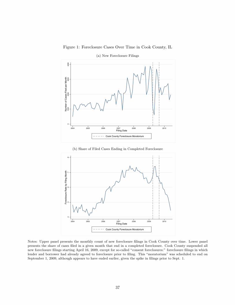
Figure 1: Foreclosure Cases Over Time in Cook County, IL

(a) New Foreclosure Filings

010

0020

0030

0040

00N

umbe

r of C

ases

File

d pe

r Mon

th

2004 2005 2006 2007 2008 2009 2010Filing Date

Cook County Foreclosure Moratorium

(b) Share of Filed Cases Ending in Completed Foreclosure

.4.5

.6.7

.8Fo

recl

osur

e R

ate

by F

iling

Mon

th

2004 2005 2006 2007 2008 2009 2010Filing Date

Cook County Foreclosure Moratorium

Notes: Upper panel presents the monthly count of new foreclosure filings in Cook County over time. Lower panelpresents the share of cases filed in a given month that end in a completed foreclosure. Cook County suspended allnew foreclosure filings starting April 16, 2009, except for so-called “consent foreclosures:” foreclosure filings in whichlender and borrower had already agreed to foreclosure prior to filing. This “moratorium” was scheduled to end onSeptember 1, 2009, although appears to have ended earlier, given the spike in filings prior to Sept. 1.

37

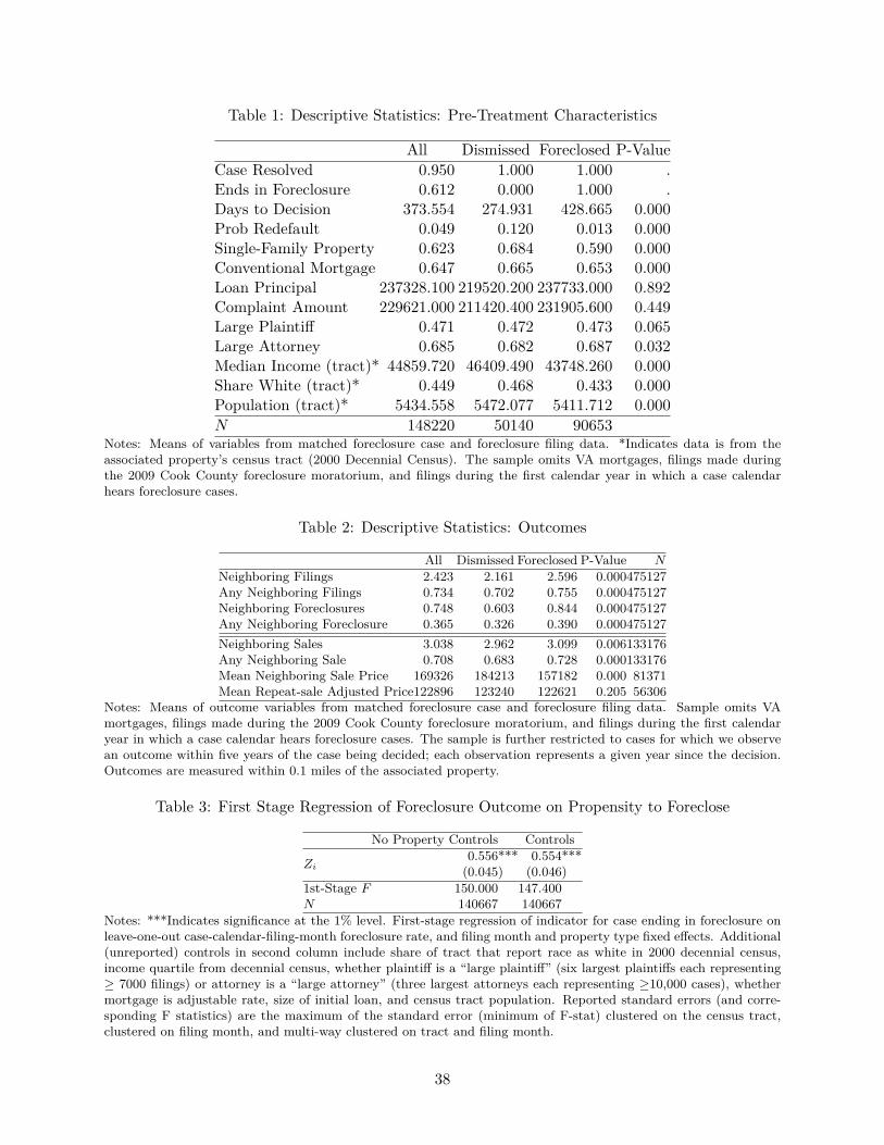
Table 1: Descriptive Statistics: Pre-Treatment Characteristics

All Dismissed Foreclosed P-ValueCase Resolved 0.950 1.000 1.000 .Ends in Foreclosure 0.612 0.000 1.000 .Days to Decision 373.554 274.931 428.665 0.000Prob Redefault 0.049 0.120 0.013 0.000Single-Family Property 0.623 0.684 0.590 0.000Conventional Mortgage 0.647 0.665 0.653 0.000Loan Principal 237328.100 219520.200 237733.000 0.892Complaint Amount 229621.000 211420.400 231905.600 0.449Large Plaintiff 0.471 0.472 0.473 0.065Large Attorney 0.685 0.682 0.687 0.032Median Income (tract)* 44859.720 46409.490 43748.260 0.000Share White (tract)* 0.449 0.468 0.433 0.000Population (tract)* 5434.558 5472.077 5411.712 0.000N 148220 50140 90653

Notes: Means of variables from matched foreclosure case and foreclosure filing data. *Indicates data is from theassociated property’s census tract (2000 Decennial Census). The sample omits VA mortgages, filings made duringthe 2009 Cook County foreclosure moratorium, and filings during the first calendar year in which a case calendarhears foreclosure cases.

Table 2: Descriptive Statistics: Outcomes

All Dismissed Foreclosed P-Value NNeighboring Filings 2.423 2.161 2.596 0.000475127Any Neighboring Filings 0.734 0.702 0.755 0.000475127Neighboring Foreclosures 0.748 0.603 0.844 0.000475127Any Neighboring Foreclosure 0.365 0.326 0.390 0.000475127Neighboring Sales 3.038 2.962 3.099 0.006133176Any Neighboring Sale 0.708 0.683 0.728 0.000133176Mean Neighboring Sale Price 169326 184213 157182 0.000 81371Mean Repeat-sale Adjusted Price122896 123240 122621 0.205 56306

Notes: Means of outcome variables from matched foreclosure case and foreclosure filing data. Sample omits VAmortgages, filings made during the 2009 Cook County foreclosure moratorium, and filings during the first calendaryear in which a case calendar hears foreclosure cases. The sample is further restricted to cases for which we observean outcome within five years of the case being decided; each observation represents a given year since the decision.Outcomes are measured within 0.1 miles of the associated property.

Table 3: First Stage Regression of Foreclosure Outcome on Propensity to Foreclose

No Property Controls Controls

Zi0.556*** 0.554***

(0.045) (0.046)1st-Stage F 150.000 147.400N 140667 140667

Notes: ***Indicates significance at the 1% level. First-stage regression of indicator for case ending in foreclosure onleave-one-out case-calendar-filing-month foreclosure rate, and filing month and property type fixed effects. Additional(unreported) controls in second column include share of tract that report race as white in 2000 decennial census,income quartile from decennial census, whether plaintiff is a “large plaintiff” (six largest plaintiffs each representing≥ 7000 filings) or attorney is a “large attorney” (three largest attorneys each representing ≥10,000 cases), whethermortgage is adjustable rate, size of initial loan, and census tract population. Reported standard errors (and corre-sponding F statistics) are the maximum of the standard error (minimum of F-stat) clustered on the census tract,clustered on filing month, and multi-way clustered on tract and filing month.

38

Table 4: Balance of Covariates

Coefficient p Value

Adj. Rate Mortgage 0.0005240 0.3837(0.0006250)

Loan Principal -0.0000033 0.0343**(0.0000025)

Large Plaintiff -0.0005760 0.9438(0.0003830)

Large Attorney -0.0007000 0.1370(0.0007400)

Median Income (tract) -0.0002720 0.6566(0.0001710)

Share White (tract) -0.0002550 0.4025(0.0005690)

Population Density (tract) 0.0558000 0.1364(0.0353000)

Price (Zip code) 0.0000507 0.8564(0.0000406)p Value 0.4280N 143276

Notes: **Indicates significance at the 5% level. First column represents the coefficient from a regression of theinstrument (case-calendar-filing-month foreclosure rate) on the given pre-treatment covariates, controlling for filingmonth and property type fixed effects. The reported p value in the first column is from a joint significance test forthe given variables. Second column reports p values from the following procedure: the given covariate (for that row)is regressed on a full set of case calendar dummies (plus filing month and property type fixed effects), where the pvalue is for a joint significance test of the case calendar dummies. For all regressions, standard errors are clusteredas in Table 3 (and the baseline 2SLS specification).

Table 5: Complier Characteristics

Quartile of Income1 2 3 4

0.785 1.012 1.059 1.066Loan Characteristics

Large Lender Conventional Positive Zip Code UnderwaterMortgage Price Growth1.002 0.896 0.794 0.781

Notes: Ratio of the first-stage estimate (effect of instrument on indicator for completed foreclosure) for given subgroupto the first-stage estimate for the full sample. Income quartile is given by the tract-level quartile of median tractincome from the 2000 Decennial Census. Large lender is an indicator for the plaintiff being one of the six mostprominent banks in the sample, each representing ≥ 10% of filings. Zip-code-level annual price growth is taken fromZillow housing price indices for Cook County. Underwater is a proxy for the outstanding balance of the mortgagebeing greater than the estimated value of the home, as described in the text.

39

Table 6: Baseline Contagion Estimates

Years Since Decision 0 1 2 3 4 5

Any Filing per Year2SLS 0.052* 0.012 0.082*** 0.090* 0.247** 0.140

(0.028) (0.027)(0.027) (0.053) (0.112) (0.133)1st-stage F 238.300 224.200 205 24.620 19.060 12.970N 130199 118566 93143 67379 41958 23831

Total Filings per Year2SLS 0.691* 0.670* 0.536*** 0.657** 1.551 0.538

(0.393) (0.368)(0.183) (0.319) (0.983) (0.987)1st-stage F 238.300 224.200 205 24.620 19.060 12.970N 130199 118566 93143 67379 41958 23831

Cumulative Effects

Cumulative Filings2SLS 0.691* 1.395* 2.090*** 4.522*** 6.446** 5.610

(0.393) (0.732)(0.794) (1.169) (3.105) (4.610)1st-stage F 238.300 224.200 205 24.620 19.060 12.970N 130199 118566 93143 67379 41958 23831

2SLS 0.622 1.266* 1.594** 3.820*** 4.076 2.693Cumulative Filings (0.380) (0.667)(0.703) (1.429) (2.918) (4.611)No Recent Foreclosures 1st-stage F 172.500 159.700 138 20.910 12.790 7.515

N 71925 66995 55105 43186 27395 14948Notes: ***Indicates significance at the 1% level, **5%, and *10%. OLS estimates of case ending in completedforeclosure on the given outcome are from a regression of the outcome . 2SLS estimates of the effect of complectedforeclosure on given outcome (measured within 0.1 miles of the property in the given year since the case is decided),on an indicator for the case ending in foreclosure, filing month, property type, and year of observation fixed effects,and case-level controls as outlined in Table 3,- instrumenting the foreclosure outcome with the leave-one-out case-calendar-filing-month-specific foreclosure rate. Standard errors and first-stage F statistics are as outlined in the notesto Table 3. Filings outcomes represent new foreclosure filings within the given radius and time period only.

Table 7: Pre-Filing Estimates

Years Before Case is Filed 3 2 1

Any Filing 0.003 0.009 0.018(0.029) (0.029) (0.022)

1st-stage F 400 400 400N 140672 140672 140672

Total Filings per Year 0.020 0.084 0.214(0.087) (0.122) (0.139)

1st-stage F 400 400 400N 140672 140672 140672

Any Completed Foreclosure -0.027 0.045* -0.004(0.023) (0.025) (0.030)

1st-stage F 159.400 182.100 164.300N 140672 140672 140672Total Completed -0.057* 0.075 0.110Foreclosures per Year (0.033) (0.065) (0.071)1st-stage F 159.400 182.100 164.300N 140672 140672 140672

log(price) 0.007 0.037 0.007(0.038) (0.042) (0.049)

1st-stage F 164.900 166.500 136.400N 109123 102220 84126

Notes: ***Indicates significance at the 1% level, **5%, and *10%. 2SLS estimates of the effect of completed foreclosureon the given outcome are from a regression of the outcome (measured within 0.1 miles of the property in the givenyear before the case is filed) on an indicator for the case ending in foreclosure (instrumented by case calendar/filingmonth foreclosure rate), filing month, property type, and year of observation fixed effects, and case-level controls asoutlined in Table 3. Standard errors and first-stage F statistics are as outlined in the notes to Table 3. Outcomesare measured as discussed in the text and in the notes to Tables 9 and 6.40

Table 8: Baseline Completed Foreclosures

Years Since Decision 0 1 2 3 4 5

Any Completed Foreclosure -0.048 0.002 0.045 0.138*** 0.033 0.174(0.031) (0.030) (0.038) (0.051) (0.106)(0.144)

First-stage F 238.300 224.200 205 24.620 19.060 12.970N 130199 118566 93143 67379 41958 23831

Total Completed Foreclosures 0.280* 0.435*** 0.312*** 0.558*** 0.243 0.063(0.164) (0.160) (0.117) (0.185) (0.316)(0.334)

First-stage F 238.300 224.200 205 24.620 19.060 12.970N 130199 118566 93143 67379 41958 23831

Contagion in Completed Foreclosures Filed Prior To Decision

Any Completed Foreclosure -0.043 0.135*** 0.073*** 0.025 -0.010 0.003(0.031) (0.028) (0.019) (0.016) (0.017)(0.015)

First-stage F 238.300 224.200 205 24.620 19.060 12.970N 130199 118566 93143 67379 41958 23831

Total Completed Foreclosures 0.303* 0.609*** 0.111*** 0.031 -0.010 0.003(0.164) (0.118) (0.028) (0.019) (0.017)(0.015)

First-stage F 238.300 224.200 205 24.620 19.060 12.970N 130199 118566 93143 67379 41958 23831

Notes: ***Indicates significance at the 1% level, **5%, and *10%. 2SLS estimates of the effect of completed foreclosureon the given outcome are from a regression of the outcome (measured within 0.1 miles of the property in the givenyear since decision) on an indicator for the case ending in foreclosure (instrumented by case calendar/filing monthforeclosure rate), filing month, property type, and year of observation fixed effects, and case-level controls as outlinedin Table 3. Standard errors and first-stage F statistics are as outlined in the notes to Table 3.

Table 9: Baseline Housing Market Estimates

Years Since Decision 0 1 2

log(price)2SLS -0.127 -0.411** -0.358

(0.105)(0.203) (0.395)1st-stage F 22.500 18.840 14.390N 43079 26047 12241

2SLS 0.059 0.003 -0.251log(price) (0.066)(0.146) (0.201)(repeat-sales) 1st-stage F 11.130 6.314 7.355

p-value 0.107 0.030 0.763N 30482 17916 7904

Any Sale2SLS 0.014 0.026 0.035

(0.046)(0.127) (0.152)1st-stage F 24.620 19.060 12.970N 67379 41958 23831

2SLS 0.220 6.562 9.964Total Sales (0.914)(4.574) (9.255)(Cumulative Over Years) 1st-stage F 24.620 19.060 12.970

N 67379 41958 23831Notes: ***Indicates significance at the 1% level, **5%, and *10%. 2SLS estimates of the effect of complectedforeclosure on given outcome (measured within 0.1 miles of the property in the given year since the case is decided),on an indicator for the case ending in foreclosure, filing month, property type, and year of observation fixed effects,and case-level controls as outlined in Table 3,- instrumenting the foreclosure outcome with the leave-one-out case-calendar-filing-month-specific foreclosure rate. Standard errors and first-stage F statistics are as outlined in thenotes to Table 3. Sales outcomes represent residential transactions within the given radius and time period only(total sales represents the total count of sales since the decision year), while price represents the mean sale price ofthese transactions. Repeat-sales adjusted prices are estimated as outlined in the text; associated p-value is for thecross-equation test of equality between the repeat-sales adjusted and unadjusted (first panel) price effects.

41

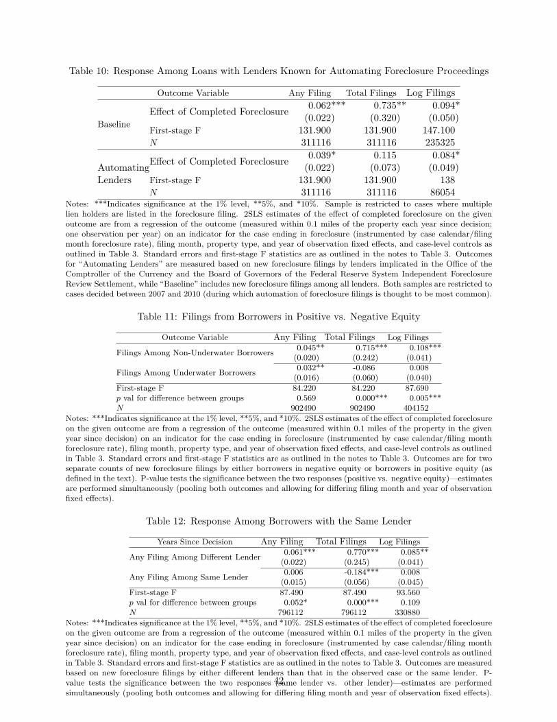
Table 10: Response Among Loans with Lenders Known for Automating Foreclosure Proceedings

Outcome Variable Any Filing Total Filings Log Filings

BaselineEffect of Completed Foreclosure 0.062*** 0.735** 0.094*

(0.022) (0.320) (0.050)First-stage F 131.900 131.900 147.100N 311116 311116 235325

Effect of Completed Foreclosure 0.039* 0.115 0.084*Automating (0.022) (0.073) (0.049)Lenders First-stage F 131.900 131.900 138

N 311116 311116 86054Notes: ***Indicates significance at the 1% level, **5%, and *10%. Sample is restricted to cases where multiplelien holders are listed in the foreclosure filing. 2SLS estimates of the effect of completed foreclosure on the givenoutcome are from a regression of the outcome (measured within 0.1 miles of the property each year since decision;one observation per year) on an indicator for the case ending in foreclosure (instrumented by case calendar/filingmonth foreclosure rate), filing month, property type, and year of observation fixed effects, and case-level controls asoutlined in Table 3. Standard errors and first-stage F statistics are as outlined in the notes to Table 3. Outcomesfor “Automating Lenders” are measured based on new foreclosure filings by lenders implicated in the Office of theComptroller of the Currency and the Board of Governors of the Federal Reserve System Independent ForeclosureReview Settlement, while “Baseline” includes new foreclosure filings among all lenders. Both samples are restricted tocases decided between 2007 and 2010 (during which automation of foreclosure filings is thought to be most common).

Table 11: Filings from Borrowers in Positive vs. Negative Equity

Outcome Variable Any Filing Total Filings Log Filings

Filings Among Non-Underwater Borrowers 0.045** 0.715*** 0.108***(0.020) (0.242) (0.041)

Filings Among Underwater Borrowers 0.032** -0.086 0.008(0.016) (0.060) (0.040)

First-stage F 84.220 84.220 87.690p val for difference between groups 0.569 0.000*** 0.005***N 902490 902490 404152

Notes: ***Indicates significance at the 1% level, **5%, and *10%. 2SLS estimates of the effect of completed foreclosureon the given outcome are from a regression of the outcome (measured within 0.1 miles of the property in the givenyear since decision) on an indicator for the case ending in foreclosure (instrumented by case calendar/filing monthforeclosure rate), filing month, property type, and year of observation fixed effects, and case-level controls as outlinedin Table 3. Standard errors and first-stage F statistics are as outlined in the notes to Table 3. Outcomes are for twoseparate counts of new foreclosure filings by either borrowers in negative equity or borrowers in positive equity (asdefined in the text). P-value tests the significance between the two responses (positive vs. negative equity)—estimatesare performed simultaneously (pooling both outcomes and allowing for differing filing month and year of observationfixed effects).

Table 12: Response Among Borrowers with the Same Lender

Years Since Decision Any Filing Total Filings Log Filings

Any Filing Among Different Lender 0.061*** 0.770*** 0.085**(0.022) (0.245) (0.041)

Any Filing Among Same Lender 0.006 -0.184*** 0.008(0.015) (0.056) (0.045)

First-stage F 87.490 87.490 93.560p val for difference between groups 0.052* 0.000*** 0.109N 796112 796112 330880

Notes: ***Indicates significance at the 1% level, **5%, and *10%. 2SLS estimates of the effect of completed foreclosureon the given outcome are from a regression of the outcome (measured within 0.1 miles of the property in the givenyear since decision) on an indicator for the case ending in foreclosure (instrumented by case calendar/filing monthforeclosure rate), filing month, property type, and year of observation fixed effects, and case-level controls as outlinedin Table 3. Standard errors and first-stage F statistics are as outlined in the notes to Table 3. Outcomes are measuredbased on new foreclosure filings by either different lenders than that in the observed case or the same lender. P-value tests the significance between the two responses (same lender vs. other lender)—estimates are performedsimultaneously (pooling both outcomes and allowing for differing filing month and year of observation fixed effects).

42

A Online Appendix—Not for Publication

A.1 Data Appendix

A.1.1 Cleaning Court Records

We collected all chancery court case records filed between January 2004 and June 2010 (inclusive).We extract from each record the associated case number and the case calendar to which the case isassigned. The records also contain a list of case actions, the lawyer who initiated this action, theassociated judge, and the date. We extract this list of actions (simple text descriptions, e.g., “Amendcomplaint or petition - allowed” or “Dismiss by stipulation or agreement”) and the correspondingdates.

We identify a case as ending in a dismissal if an action occurs containing one of the followingdescriptions: "mortgage foreclosure motion plaintiff dismissed", "mortgage foreclosure voluntarydismissal, non-suit or dismiss by agreement", "mortgage foreclosure motion defendant dismissed","mortgage foreclosure dismissed for want of prosecution", "dismissed for want of prosecution", "gen-eral chancery - dismissed for want of prosecution", "general chancery - voluntary dismissal, nonsuit, dismiss by agreement", "mortgage foreclosure voluntary dismissal, non-suit or dismiss byagreement", or "mortgage foreclosure judgment for defendant"; or an action containing any of thefollowing: "case dismissed", "voluntary dismissal", "declaratory judgment voluntary dismissal", "dis-miss entire cause" and not "denied", or "dismiss by stipulation or agreement" and not "denied". Fordismissed cases, we consider the end of the case to be the date of this “dismissal” action (in thecase of multiple such actions, we take the final).

A.1.2 Cleaning RIS Data

Record Information Services, Inc. provided us with details of foreclosure filings and foreclosureauctions for Cook County from 2002 through 2011. RIS is a private data provision company thatcollects publicly available records on all foreclosure filings in the five counties of Chicago. RISemployees manually input data on each foreclosure filing. From the foreclosure filings, we extractthe associated chancery court case number, unique loan ID, the filing date, details of the associatedloan (origination date, principal at origination, outstanding claim at time of foreclosure filing, ageneral indication of mortgage type—conventional, adjustable rate, etc.), details of the associatedproperty (latitude and longitude, census tract, zip code, property type—condo, single family, etc.),and the parties involved (defendant name, plaintiff—the lender or servicer—identity, plaintiff lawfirm).

We identify a case as ending in a completed foreclosure if there is an associated foreclosureauction record in the RIS data. For completed foreclosures, we use the date of the foreclosureauction as the end-date of the case. If there is both a dismissal action in the court records andan associated foreclosure auction, we consider the case to have ended in a completed foreclosure,although, our results are not sensitive to this decision. Relatedly, there is a field in the RIS data that

43

indicates the outcome of the auction, including if the auction is canceled. Since this information ismissing for half of the years and since it is not indicated why a cancellation occurs, we do not codecanceled auctions as dismissals in our analysis sample. Again, however, our baseline results are notsensitive to coding canceled auctions as dismissals. We consider a borrower to have redefaulted ifa foreclosure filing is brought against the same loan ID. Note that this will not count new filingsat the same property for different loans (e.g., if the home owner has filings against mortgage and ahome equity loan, we count these as distinct filings). However, if a second filing against the sameloan ID occurs within 180 days of the initial filing, we consider this to be the same case, taking thefirst date as the true filing date (and merging info from the two filings).

We construct a unique ID for each plaintiff and attorney as follows. For plaintiffs and attorneyson more than ∼100 cases, we manually checked the names for consistency and constructed a uniqueID number. We then identified “large plaintiffs” as those plaintiff-IDs associated with greater than7000 cases, and “large attorneys” as those attorney-IDs associated with greater than 10000 cases.We identify by name all plaintiffs implicated in the Independent Foreclosure Review Settlementconducted by the Office of the Comptroller of the Currency and the Board of Governors of theFederal Reserve System.

We match the RIS and chancery court records by case number. We discard non-matches, whicharise due to several factors: non-foreclosure chancery court cases (e.g., name changes, mechanic’sliens) will not appear in the RIS foreclosure filings; differing date ranges between the two datasources (2004–2010 for court records, 2002–2011 for RIS); and differing geographies (RIS dataincludes some cases in neighboring counties).

A.1.3 Cleaning Census Data

We merge in the following census-tract-level data from the 2000 Decennial Census: median tractincome, population, land area, and share of population that identifies as each census-designatedrace. We construct tract-level income quartiles (i.e., what quartile of median income does a giventract fall into), an indicator for being a predominantly white tract (share white is greater than themedian share), population density (and associated quartiles), and a Herfindahl-Hirschman indexfor each race (i.e., the sum of the squared share of each race in the tract). We merge the censustract data to the RIS data using census tract FIPS codes.

A.1.4 Cleaning Deeds Records

These data are collected from the county recorder for Cook County, IL. The records were collectedby an anonymous private firm and made available to us by the Paul Millstein Center for RealEstate at the Columbia Graduate School of Business. These data include the date of each saleproperty transaction, the type of property, the address, the price of the sale, and an indicator forthe property being residential. We drop all transactions with sale price or address missing. Wedrop duplicate records—multiple sales with identical sale prices that occur at the same property

44

within 30 days of one another. We keep only residential sales. We geocode these deeds recordsbased on the property address using Yahoo! Placefinder.

A.1.5 Defining Outcomes

Using the cleaned and matched RIS and court records, for each foreclosure case we calculate thedistance between the associated property and the properties associated with all other foreclosurefilings. We then count the number of new filings around each property (i.e., within the givenradius; 0.1 miles in the baseline) in each calendar year, omitting from the count new filings at thesame property or filings associated with the same case—e.g., a given loan may be tied to multipleproperties, which we do not want to include in the count. If there are multiple foreclosure filingsat a neighboring property, we include each of these in the count (although we have found that ourresults are not sensitive to treating these as a single new filing). For each calendar year, we thenconstruct an indicator for there being any new foreclosure filing. We then identify the year thatthe case is decided and define our contagion outcomes relative to that year: number of filings andindicator for any filing in the year the case ends, number and indicator one year after the caseends, two years after, and so on. We follow the same procedure to get a count of new completedforeclosures in each calendar year: calculate the distance between the property associated witheach case and each completed foreclosure (from the RIS auction data), and count the auctions thatoccur within the given radius in the given calendar year (where this date is based on the auctiondate).

We also construct several sub-counts of new foreclosure filings. Foreclosure filing records inthe RIS data have a field reporting additional lien holders that are listed on the foreclosure claim(reporting additional lien holders is optional for plaintiffs). For each filing we create an indicatorfor additional lien holders. We then construct the same contagion outcomes, but only countingfilings with multiple lien holders. Similarly, we construct our contagion outcomes using the annualcount of new filings from plaintiffs implicated in the Independent Foreclosure Review Settlementand, as described in the text, use this to investigate contagion among lenders known for the bulkprocessing of delinquent loans into foreclosure filings. Thirdly, we construct an indicator for theborrower being underwater on their loan: we take the principal of the mortgage at origination,conservatively assume an 80% loan-to-value ratio to back out the value of the property, adjust thevalue of the property using Zillow monthly zip code housing price indices for the year of originationand the year of the foreclosure filing, and compare the adjusted value of the property to the claimmade against the borrower by the plaintiff. If the claim is larger than the value of the property,then we consider the borrower to be “underwater”. For each property associated with a foreclosurefiling, we then find the annual count of filings against underwater borrowers within the given radius.We have experimented with other ways to construct this underwater indicator—claim larger thanloan principal at origination, claim larger than 110% of estimated value, and so on—and find littledifference in our results. Finally, we construct contagion outcomes for filings from the same lender.We restrict our sample to the set of cases for which we cleaned the plaintiff name (i.e., filings with

45

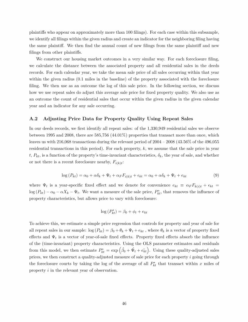
plaintiffs who appear on approximately more than 100 filings). For each case within this subsample,we identify all filings within the given radius and create an indicator for the neighboring filing havingthe same plaintiff. We then find the annual count of new filings from the same plaintiff and newfilings from other plaintiffs.

We construct our housing market outcomes in a very similar way. For each foreclosure filing,we calculate the distance between the associated property and all residential sales in the deedsrecords. For each calendar year, we take the mean sale price of all sales occurring within that yearwithin the given radius (0.1 miles in the baseline) of the property associated with the foreclosurefiling. We then use as an outcome the log of this sale price. In the following section, we discusshow we use repeat sales do adjust this average sale price for fixed property quality. We also use asan outcome the count of residential sales that occur within the given radius in the given calendaryear and an indicator for any sale occurring.

A.2 Adjusting Price Data for Property Quality Using Repeat Sales

In our deeds records, we first identify all repeat sales: of the 1,330,949 residential sales we observebetween 1995 and 2008, there are 585,756 (44.01%) properties that transact more than once, whichleaves us with 216,068 transactions during the relevant period of 2004 – 2008 (43.56% of the 496,055residential transactions in this period). For each property, k, we assume that the sale price in yeart, Pkt, is a function of the property’s time-invariant characteristics, δk, the year of sale, and whetheror not there is a recent foreclosure nearby, Fi(k)t:

log (Pkt) = α0 + αδk + Ψt + αF Fi(k)t + �kt = α0 + αδk + Ψt + ekt (9)

where Ψt is a year-specific fixed effect and we denote for convenience ekt ≡ αF Fk(i)t + �kt =log (Pkt) − α0 − αXk − Ψt. We want a measure of the sale price, P

∗kt, that removes the influence of

property characteristics, but allows price to vary with foreclosure:

log (P ∗kt) = β0 + φt + ekt

To achieve this, we estimate a simple price regression that controls for property and year of sale forall repeat sales in our sample: log (Pkt) = β0 + θk + Ψt + ekt , where θk is a vector of property fixedeffects and Ψt is a vector of year-of-sale fixed effects. Property fixed effects absorb the influenceof the (time-invariant) property characteristics. Using the OLS parameter estimates and residualsfrom this model, we then estimate P

∗kt = exp

�β0 + Ψt + ekt

�. Using these quality-adjusted sales

prices, we then construct a quality-adjusted measure of sale price for each property i going throughthe foreclosure courts by taking the log of the average of all P

∗kt that transact within x miles of

property i in the relevant year of observation.

46

A.3 Monotonicity of Instrument

A failure of monotonicity occurs if a higher value of the instrument means a higher probabilityof foreclosure for some cases, but a lower probability for others. As discussed in the main text, afailure of monotonicity may arise if judges treat different types of borrowers and lenders differently.

We examine this possibility by relating foreclosure rates for each case calendar for differentsubgroups to the overall value of the instrument for that case calendar. We want to check that ahigher value of the instrument for the case calendar is associated with a higher foreclosure rate forthe sub-groups. We first calculate the overall foreclosure rate by case calendar and filing year, andde-mean these estimates by filing year. 41We then take a given covariate (e.g., the borrower is froma predominantly white neighborhood) and calculate the foreclosure rate by case calendar, filingyear, and the value of the covariate (e.g., foreclosure rate by case calendar, filing year, and whetherpredominantly white neighborhood), and again de-mean by filing year. We plot the de-meanedgroup-specific foreclosure rates against the de-meaned general case-calendar-filing-year foreclosurerate and display these plots in Figures A.1 and A.2. A failure of monotonicity as we described abovesuggests that for certain subgroups a higher general case-calendar foreclosure rate is associated witha higher group-specific foreclosure rate, while for other subgroups a higher general case-calendarforeclosure rate is associated with a lower group-specific foreclosure rate. We construct six suchplots: i) comparing foreclosure rates between properties in census tracts where the share of whiteresidents is greater than the median to those below the median, ii) comparing properties in eachquartile of median tract-level income, iii) comparing foreclosure rates among conventional (fixed-rate) mortgages vs. unconventional mortgages (adjustable rate, interest only, etc.), iv) comparingforeclosure rates by property type, v) comparing cases where the plaintiff is a large lender to thosewith smaller lenders, and vi) comparing foreclosure rates among cases where the lender’s attorneyis a large vs. smaller attorney (as previously defined). Figure A.1 shows that there is no evidenceof a failure of monotonicity. In all cases, there is a clear positive relationship between the overallcase-calendar-filing-year foreclosure rate and the group-specific case-calendar-filing-year foreclosurerate—a higher value of the instrument is associated with a higher foreclosure rate in each subgroup.Thus, in terms of observables—property type, loan type, whether the plaintiff is a large bank oremploys a large attorney, and census tract demographics—the monotonicity assumption appearsvalid.

A.4 Lender Response to a Completed Foreclosure

For any given mortgage, divide the remaining life of the loan into three periods (t ∈ 0, 1, 2). Considera mortgage in which the borrower owes a payment of mt in each period, t and the mortgage is fullypaid back as of t = 2. Suppose the borrower misses their payment in the current period (t = 0).With probability α1 the borrower will still be delinquent the following period and the lender can

41Recall that our estimates all include filing date fixed effects, so the relevant comparison is within filing date,although the figures are similar if we do not de-mean. We use filing year for this exercise to decrease noise in theforeclosure rate estimates; the story does not change if we use filing month, although the associated figures are noisier.

47

foreclose on the property, in which case the lender recovers the value of the home, P , less the costsof foreclosure, λ (e.g., legal fees). However, with probability 1 − α1, the borrower will recover inperiod 1 and will resume making payments. Then the value of the unmodified loan to the lenderis:

Vu = α1 · (P − λ) + (1 − α1) ·�m1 + m2

R

�(10)

where R is the discount rate. The lender may instead choose to modify the loan, which reducessubsequent loan payments to m

�1 < m1 and m

�2 < m2.

Lenders will be willing to modify a mortgage when modification is very effective in reducing theprobability of non-payment or when the necessary reduction in the value of the loan is small. Bylowering payments, modification reduces the probability of default to α

�1 < α1.42Then the value of

the modified loan is:

VM = α�1(P − λ) + (1 − α

�1)

�m

�1 + m

�2

R

�

Thus, the lender will choose modification when the value of the modified loan is larger than theunmodified loan, or the difference between the two is positive:

VM − Vu = (α1 − α�1) ·

�m

�1 + 1

Rm

�2 − (P − λ)

�− (1 − α1) ·

�m1 + 1

Rm2 − (m�

1 + 1R

m�2)

�> 0 (11)

Since α1 − α�1 > 0 , 1 − α1 > 0, and

�m1 + 1

Rm2 − (m�1 + 1

Rm�2)

�> 0, even if the probability of

re-default under modification is zero (i.e., even if α�1 = 0), modification is still not optimal if the

modified payments are too low. For example, lenders will never modify if the net-of-foreclosure-costvalue of the property is greater than the present value of the modified mortgage payments (i.e.,m

�1 + 1

Rm�2 < (P − λ)). When the value of the modified payments are high enough, lenders are

more inclined to modify when it is very effective in reducing the probability of redefault (i.e., thesmaller is α

�1).

Assuming that the default probabilities are constant (which shuts down the borrower contagionchannel), a neighboring completed home foreclosure—which lowers the value of the property underconsideration—discourages new foreclosure filings by lenders. Taking the derivative of VM −Vu withrespect to the value of the home, we see that ∂VM −Vu

∂P = α�1 −α1 < 0, relying on the assumption that

modification lowers the probability of future default. A drop in the value of the home encouragesmortgage modification—selling the property at auction is relatively less appealing to the lenderthan the modified mortgage.

We derive similar conditions for modification by mortgage servicers. Mortgage servicers are42Adelino et al. (2009) allow home prices to change across periods, however, for the purpose of this paper little

generality is lost by assuming no price growth. Similarly, Adelino et al. (2009) operate under the assumption thatmodification guarantees payment in period 1 with a non-zero probability of default in period 2. Again, this does notfundamentally change the implications of the framework.

48

typically employed by lenders to collect mortgage payments and to manage mortgage defaults.When a mortgage is current, servicers receive a share of the interest payments that they collect.However, when a borrower is delinquent, servicers are required to forward payments to the holderof the debt while they manage the default (either by modifying the loan or seeking foreclosure).While managing a default, the servicer must incur all associated costs (e.g. legal fees). If thedefault ends in foreclosure, the servicer is reimbursed for all foreclosure-related expenses and fees.Thus, the value to the servicer of foreclosing on the delinquent loan (as in the above framework) is:

Vs

u = α1 · Π + (1 − α1) ·�ρ · m1 + ρ · m2

R

�(12)

where Π is the total value of all foreclosure-related fees charged by the servicer and where ρ is theshare of the mortgage payment that is returned to the servicer. When the loan is modified, theservicer is generally not reimbursed for any related expenses, and so the value of the modified loanto the servicer is:

Vs

M = α�1 · Π + (1 − α

�1)

�ρ · m

�1 + ρ · m

�2

R

�− CM

where CM is the cost of modification (e.g., time/labor spent in negotiations). Notice that if themodification is successful, the servicer receives a lower monthly payment for servicing the mortgage.Then the servicer will prefer to modify when:

Vs

M − Vs

u = (α�1 − α1) ·

�ρm

�1 + ρ

Rm

�2 − Π

�− (1 − α1) · ρ

�m1 + 1

Rm2 −

�m

�1 + 1

Rm

�2

��− Cm > 0

The servicer’s incentives are similar to the lender’s incentives, although as pointed out by Levitinand Twomey (2011), since servicers’ fees have seniority over all other claims against a property,servicers are “indifferent to the amount of the [foreclosure] sale proceeds.” In other words, since thepayoff to a servicer of a completed foreclosure is the foreclosure fees, the servicer does not care aboutthe value of the property (as long as it is high enough to cover their fees). Moreover, high costsof modification (which are not reimbursed) will push the servicer in favor of foreclosure. Notice,then, that if the probabilities of foreclosure (α1 and α

�1) are invariant to a neighboring completed

foreclosure, the servicer will not experience foreclosure contagion (∂ (V sM − V

su ) /∂P = 0).

In summary, under the assumptions that a neighboring completed home foreclosure lowers thehousing value P and that borrowers are unresponsive to the neighboring foreclosure so that α1

and α�1 are unchanged, we should observe “anti-contagion” in home foreclosures: if only lenders

and servicers are responding, a completed home foreclosure should discourage neighboring foreclo-sure filings. Of course, if a neighboring completed foreclosure has no influence on housing valuesand borrowers are unresponsive, then lenders and servicers should not respond (we should see nocontagion at all).

49

A.5 Estimates by Proxies for Social Connectedness

We find little systematic relationship between the extent of foreclosure contagion and several proxiesfor social connection. Our first attempt to proxy social connectedness is to stratify by neighborhooddiversity, operating under the assumption that neighbors with similar background maintain strongersocial ties. For each census tract, we calculate a Herfindahl index of neighborhood diversity usingrace-population shares from the 2000 Decennial Census. We then estimate the baseline treatmenteffect for each diversity quartile to examine whether contagion is stronger in less diverse (high-index)census tracts. We also estimate the baseline specification and interact the treatment effect with anindicator for the foreclosure taking place in a census tract where a single race makes up more than75% of the population. Our second set of proxies draw on the notion of social capital outlined byGlaeser and Sacerdote (2000), who argue that social connections are higher when residents live inclose proximity to one another. For example, studying survey data, Glaeser and Sacerdote (2000)find that there are higher levels of civic participation among residents of large condo buildings thansingle-family housing. We proxy neighbor proximity in two ways. First, we interact the foreclosuretreatment effect with an indicator that the home undergoing foreclosure (the unit of observation)is a condominium unit. Second, we stratify census tracts by population density (again using datafrom the 2000 Decennial Census). In both of these cases, while we continue to find evidence ofcontagion, there is no systematic relationship between foreclosure contagion and our proxies forsocial connection. Our social-contagion estimates can be found in Table A.16 and Figure A.3 ofthe Appendix.

50

51

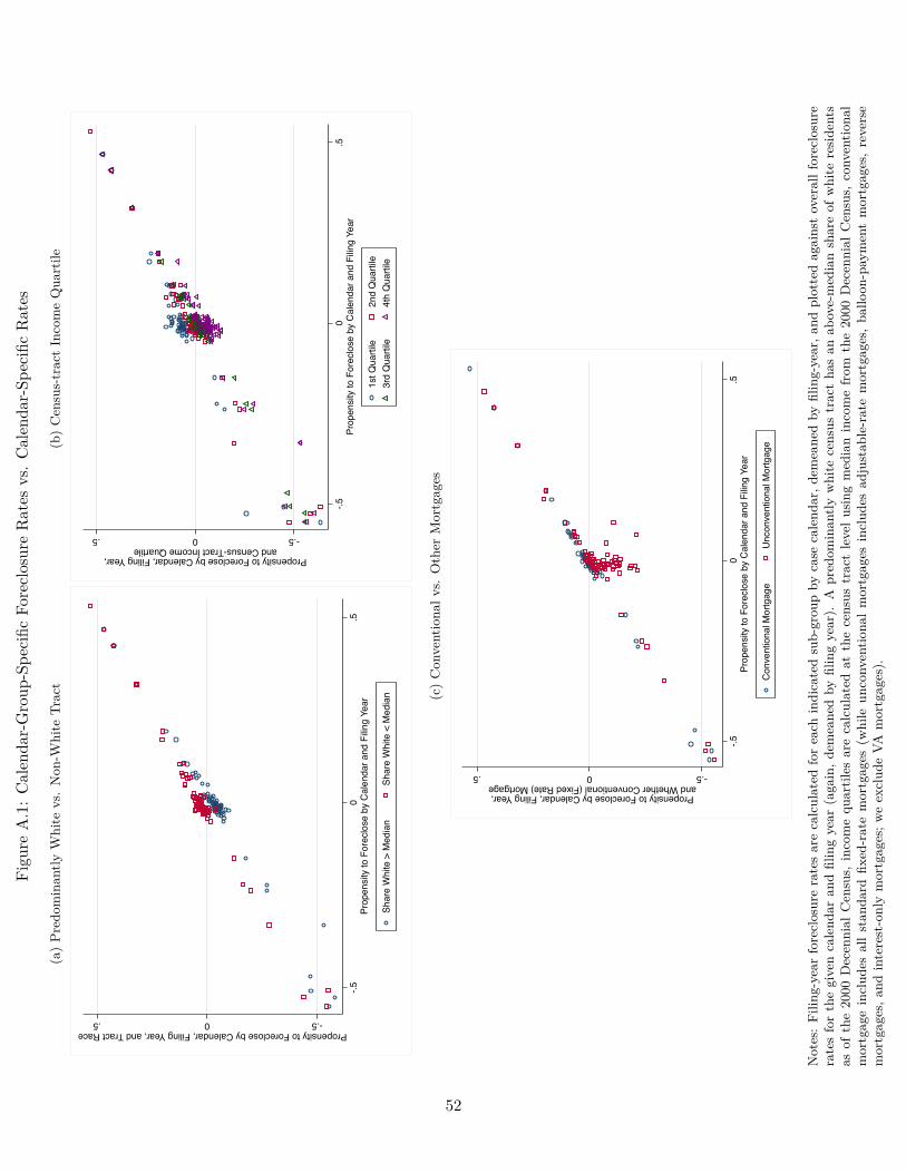
Figu

reA

.1:

Cal

enda

r-G

roup

-Spe

cific

Fore

clos

ure

Rat

esvs

.C

alen

dar-

Spec

ific

Rat

es

(a)

Pred

omin

antly

Whi

tevs

.N

on-W

hite

Trac

t

-.50.5Propensity to Foreclose by Calendar, Filing Year, and Tract Race

-.50

.5Pr

open

sity

to F

orec

lose

by

Cal

enda

r and

Filin

g Ye

ar

Shar

e W

hite

> M

edia

nSh

are

Whi

te <

Med

ian

(b)

Cen

sus-

trac

tIn

com

eQ

uart

ile

-.50.5

Propensity to Foreclose by Calendar, Filing Year,and Census-Tract Income Quartile

-.50

.5Pr

open

sity

to F

orec

lose

by

Cal

enda

r and

Filin

g Ye

ar

1st Q

uarti

le2n

d Q

uarti

le3r

d Q

uarti

le4t

h Q

uarti

le

(c)

Con

vent

iona

lvs.

Oth

erM

ortg

ages

-.50.5

Propensity to Foreclose by Calendar, Filing Year,and Whether Conventional (Fixed Rate) Mortgage

-.50

.5Pr

open

sity

to F

orec

lose

by

Cal

enda

r and

Filin

g Ye

ar

Con

vent

iona

l Mor

tgag

eU

ncon

vent

iona

l Mor

tgag

e

Not

es:

Filin

g-ye

arfo

recl

osur

era

tes

are

calc

ulat

edfo

rea

chin

dica

ted

sub-

grou

pby

case

cale

ndar

,dem

eane

dby

filin

g-ye

ar,a

ndpl

otte

dag

ains

tov

eral

lfor

eclo

sure

rate

sfo

rth

egi

ven

cale

ndar

and

filin

gye

ar(a

gain

,dem

eane

dby

filin

gye

ar).

Apr

edom

inan

tlyw

hite

cens

ustr

act

has

anab

ove-

med

ian

shar

eof

whi

tere

siden

tsas

ofth

e20

00D

ecen

nial

Cen

sus,

inco

me

quar

tiles

are

calc

ulat

edat

the

cens

ustr

act

leve

lusin

gm

edia

nin

com

efr

omth

e20

00D

ecen

nial

Cen

sus,

conv

entio

nal

mor

tgag

ein

clud

esal

lst

anda

rdfix

ed-r

ate

mor

tgag

es(w

hile

unco

nven

tiona

lm

ortg

ages

incl

udes

adju

stab

le-r

ate

mor

tgag

es,

ballo

on-p

aym

ent

mor

tgag

es,

reve

rse

mor

tgag

es,a

ndin

tere

st-o

nly

mor

tgag

es;w

eex

clud

eVA

mor

tgag

es).

52

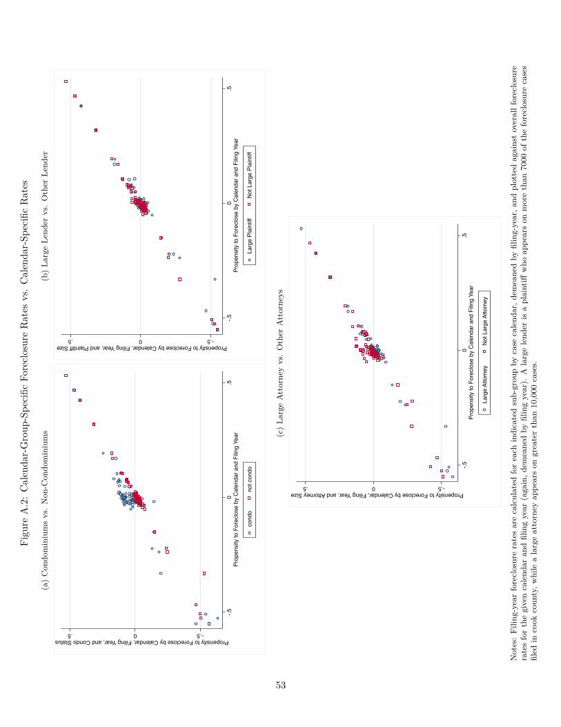
Figu

reA

.2:

Cal

enda

r-G

roup

-Spe

cific

Fore

clos

ure

Rat

esvs

.C

alen

dar-

Spec

ific

Rat

es

(a)

Con

dom

iniu

ms

vs.

Non

-Con

dom

iniu

ms

-.50.5Propensity to Foreclose by Calendar, Filing Year, and Condo Status

-.50

.5Pr

open

sity

to F

orec

lose

by

Cal

enda

r and

Filin

g Ye

ar

cond

ono

t con

do

(b)

Larg

eLe

nder

vs.

Oth

erLe

nder

-.50.5Propensity to Foreclose by Calendar, Filing Year, and Plaintiff Size

-.50

.5Pr

open

sity

to F

orec

lose

by

Cal

enda

r and

Filin

g Ye

ar

Larg

e Pl

aint

iffN

ot L

arge

Pla

intif

f

(c)

Larg

eA

ttor

ney

vs.

Oth

erA

ttor

neys

-.50.5Propensity to Foreclose by Calendar, Filing Year, and Attorney Size

-.50

.5Pr

open

sity

to F

orec

lose

by

Cal

enda

r and

Filin

g Ye

ar

Larg

e At

torn

eyN

ot L

arge

Atto

rney

Not

es:

Filin

g-ye

arfo

recl

osur

era

tes

are

calc

ulat

edfo

rea

chin

dica

ted

sub-

grou

pby

case

cale

ndar

,dem

eane

dby

filin

g-ye

ar,a

ndpl

otte

dag

ains

tov

eral

lfor

eclo

sure

rate

sfo

rth

egi

ven

cale

ndar

and

filin

gye

ar(a

gain

,dem

eane

dby

filin

gye

ar).

Ala

rge

lend

eris

apl

aint

iffw

hoap

pear

son

mor

eth

an70

00of

the

fore

clos

ure

case

sfil

edin

cook

coun

ty,w

hile

ala

rge

atto

rney

appe

ars

ongr

eate

rth

an10

,000

case

s.

53

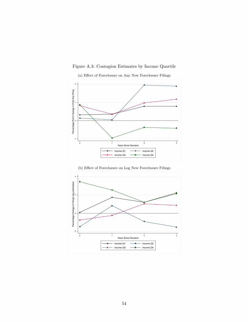
Figure A.3: Contagion Estimates by Income Quartile

(a) Effect of Foreclosure on Any New Foreclosure Filings-.1

0.1

.2Pe

rcen

tage

-Poi

nt C

hang

e in

Pro

b An

y Fi

ling

0 1 2 3Years Since Decision

Income Q1 Income Q2Income Q3 Income Q4

(b) Effect of Foreclosure on Log New Foreclosure Filings

-.20

.2.4

Perc

enta

ge-C

hang

e in

Filin

gs (l

og e

stim

ates

)

0 1 2 3Years Since Decision

Income Q1 Income Q2Income Q3 Income Q4

54

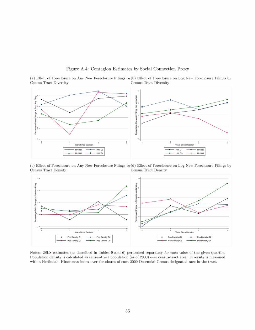
Figure A.4: Contagion Estimates by Social Connection Proxy

(a) Effect of Foreclosure on Any New Foreclosure Filings byCensus Tract Diversity

-.1-.0

50

.05

.1Pe

rcen

tage

-Poi

nt C

hang

e in

Pro

b An

y Fi

ling

0 1 2 3Years Since Decision

HHI Q1 HHI Q2HHI Q3 HHI Q4

(b) Effect of Foreclosure on Log New Foreclosure Filings byCensus Tract Diversity

-.4-.2

0.2

.4Pe

rcen

tage

-Cha

nge

in F

ilings

(log

est

imat

es)

0 1 2 3Years Since Decision

HHI Q1 HHI Q2HHI Q3 HHI Q4

(c) Effect of Foreclosure on Any New Foreclosure Filings byCensus Tract Density

-.10

.1.2

.3Pe

rcen

tage

-Poi

nt C

hang

e in

Pro

b An

y Fi

ling

0 1 2 3Years Since Decision

Pop Density Q1 Pop Density Q2Pop Density Q3 Pop Density Q4

(d) Effect of Foreclosure on Log New Foreclosure Filings byCensus Tract Density

-.10

.1.2

.3.4

Perc

enta

ge-C

hang

e in

Filin

gs (l

og e

stim

ates

)

0 1 2 3Years Since Decision

Pop Density Q1 Pop Density Q2Pop Density Q3 Pop Density Q4

Notes: 2SLS estimates (as described in Tables 9 and 6) performed separately for each value of the given quartile.Population density is calculated as census-tract population (as of 2000) over census-tract area. Diversity is measuredwith a Herfindahl-Hirschman index over the shares of each 2000 Decennial Census-designated race in the tract.

55

56

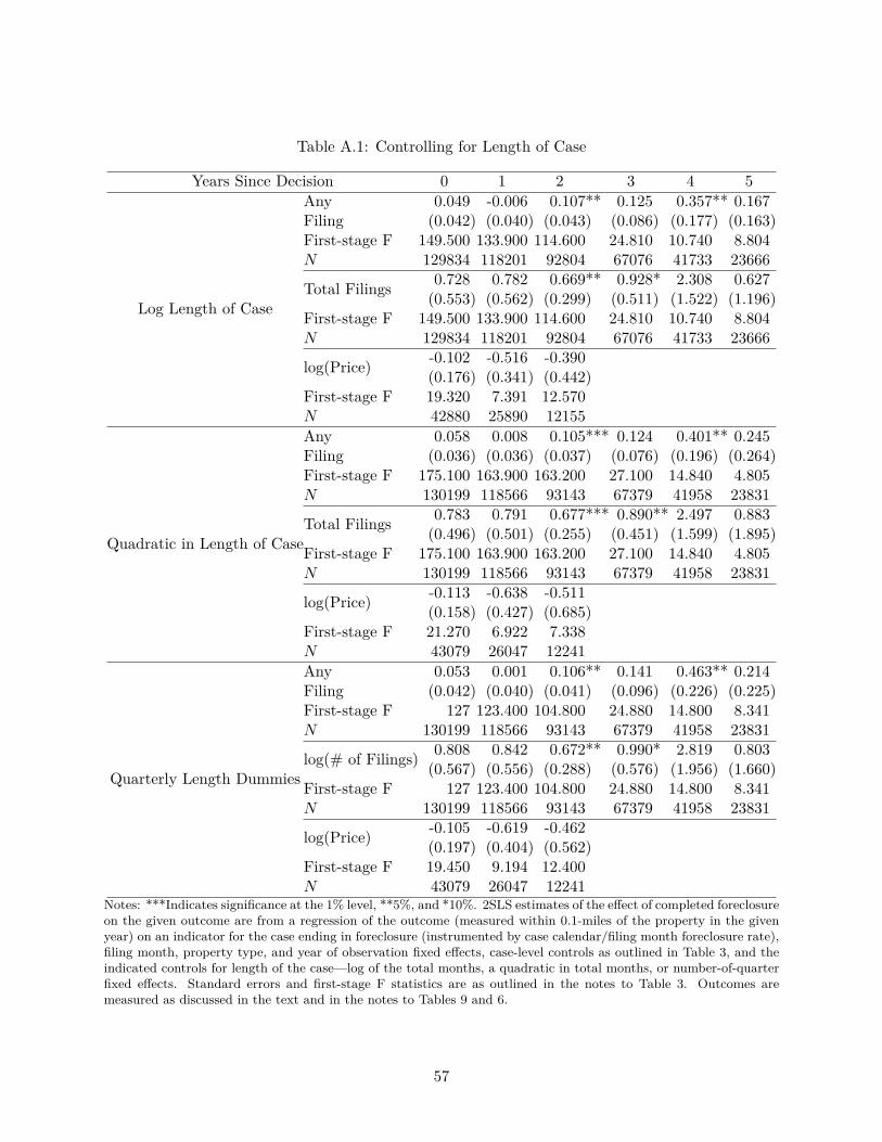
Table A.1: Controlling for Length of Case

Years Since Decision 0 1 2 3 4 5Any 0.049 -0.006 0.107** 0.125 0.357** 0.167

Log Length of Case

Filing (0.042) (0.040) (0.043) (0.086) (0.177) (0.163)First-stage F 149.500 133.900 114.600 24.810 10.740 8.804N 129834 118201 92804 67076 41733 23666

Total Filings 0.728 0.782 0.669** 0.928* 2.308 0.627(0.553) (0.562) (0.299) (0.511) (1.522) (1.196)

First-stage F 149.500 133.900 114.600 24.810 10.740 8.804N 129834 118201 92804 67076 41733 23666

log(Price) -0.102 -0.516 -0.390(0.176) (0.341) (0.442)

First-stage F 19.320 7.391 12.570N 42880 25890 12155Any 0.058 0.008 0.105*** 0.124 0.401** 0.245

Quadratic in Length of Case

Filing (0.036) (0.036) (0.037) (0.076) (0.196) (0.264)First-stage F 175.100 163.900 163.200 27.100 14.840 4.805N 130199 118566 93143 67379 41958 23831

Total Filings 0.783 0.791 0.677*** 0.890** 2.497 0.883(0.496) (0.501) (0.255) (0.451) (1.599) (1.895)

First-stage F 175.100 163.900 163.200 27.100 14.840 4.805N 130199 118566 93143 67379 41958 23831

log(Price) -0.113 -0.638 -0.511(0.158) (0.427) (0.685)

First-stage F 21.270 6.922 7.338N 43079 26047 12241Any 0.053 0.001 0.106** 0.141 0.463** 0.214

Quarterly Length Dummies

Filing (0.042) (0.040) (0.041) (0.096) (0.226) (0.225)First-stage F 127 123.400 104.800 24.880 14.800 8.341N 130199 118566 93143 67379 41958 23831

log(# of Filings) 0.808 0.842 0.672** 0.990* 2.819 0.803(0.567) (0.556) (0.288) (0.576) (1.956) (1.660)

First-stage F 127 123.400 104.800 24.880 14.800 8.341N 130199 118566 93143 67379 41958 23831

log(Price) -0.105 -0.619 -0.462(0.197) (0.404) (0.562)

First-stage F 19.450 9.194 12.400N 43079 26047 12241

Notes: ***Indicates significance at the 1% level, **5%, and *10%. 2SLS estimates of the effect of completed foreclosureon the given outcome are from a regression of the outcome (measured within 0.1-miles of the property in the givenyear) on an indicator for the case ending in foreclosure (instrumented by case calendar/filing month foreclosure rate),filing month, property type, and year of observation fixed effects, case-level controls as outlined in Table 3, and theindicated controls for length of the case—log of the total months, a quadratic in total months, or number-of-quarterfixed effects. Standard errors and first-stage F statistics are as outlined in the notes to Table 3. Outcomes aremeasured as discussed in the text and in the notes to Tables 9 and 6.

57

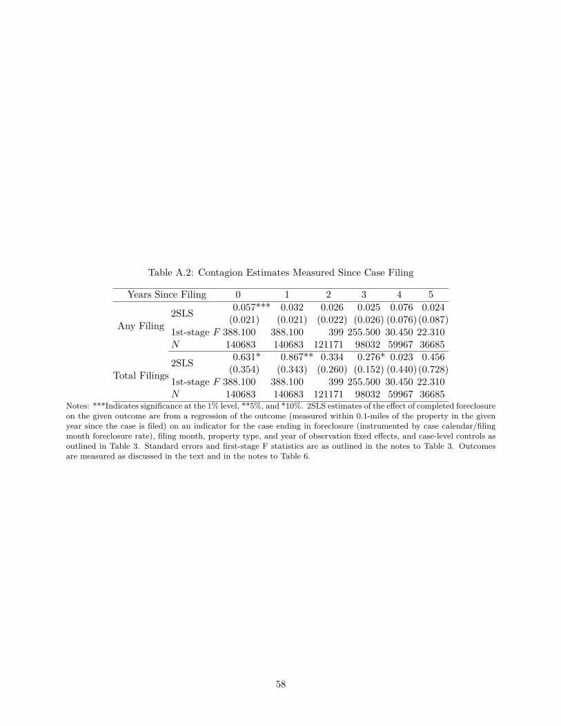
Table A.2: Contagion Estimates Measured Since Case Filing

Years Since Filing 0 1 2 3 4 5

Any Filing2SLS 0.057*** 0.032 0.026 0.025 0.076 0.024

(0.021) (0.021) (0.022) (0.026) (0.076)(0.087)1st-stage F 388.100 388.100 399 255.500 30.450 22.310N 140683 140683 121171 98032 59967 36685

Total Filings2SLS 0.631* 0.867** 0.334 0.276* 0.023 0.456

(0.354) (0.343) (0.260) (0.152) (0.440)(0.728)1st-stage F 388.100 388.100 399 255.500 30.450 22.310N 140683 140683 121171 98032 59967 36685

Notes: ***Indicates significance at the 1% level, **5%, and *10%. 2SLS estimates of the effect of completed foreclosureon the given outcome are from a regression of the outcome (measured within 0.1-miles of the property in the givenyear since the case is filed) on an indicator for the case ending in foreclosure (instrumented by case calendar/filingmonth foreclosure rate), filing month, property type, and year of observation fixed effects, and case-level controls asoutlined in Table 3. Standard errors and first-stage F statistics are as outlined in the notes to Table 3. Outcomesare measured as discussed in the text and in the notes to Table 6.

58

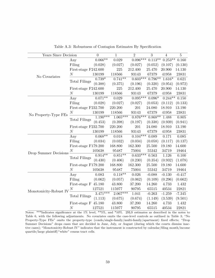
Table A.3: Robustness of Contagion Estimates By Specification

Years Since Decision 0 1 2 3 4 5Any 0.066** 0.029 0.096*** 0.113** 0.253** 0.160

No Covariates

Filing (0.028) (0.027) (0.027) (0.052) (0.107) (0.130)First-stage F242.600 225 212.400 25.470 20.900 14.130N 130199 118566 93143 67379 41958 23831

Total Filings 0.739* 0.741** 0.603*** 0.796** 1.616* 0.621(0.388) (0.375) (0.196) (0.320) (0.954) (0.972)

First-stage F242.600 225 212.400 25.470 20.900 14.130N 130199 118566 93143 67379 41958 23831Any 0.071** 0.029 0.095*** 0.096* 0.244** 0.150

No Property-Type FEs

Filing (0.028) (0.027) (0.027) (0.053) (0.112) (0.133)First-stage F232.700 220.200 201 24.080 18.910 13.190N 130199 118566 93143 67379 41958 23831

Total Filings 1.190*** 1.065*** 0.876*** 0.868** 1.488 0.805(0.453) (0.398) (0.197) (0.338) (0.939) (0.941)

First-stage F232.700 220.200 201 24.080 18.910 13.190N 130199 118566 93143 67379 41958 23831Any 0.068** 0.018 0.104*** 0.089 0.171 0.085

Drop Summer Decisions

Filing (0.034) (0.032) (0.034) (0.058) (0.117) (0.137)First-stage F179.200 168.800 162.300 25.500 19.180 14.600N 105638 95487 75004 55342 34719 19464

Total Filings 0.914** 0.851** 0.633*** 0.563 1.126 0.100(0.430) (0.406) (0.230) (0.354) (0.932) (1.078)

First-stage F179.200 168.800 162.300 25.500 19.180 14.600N 105638 95487 75004 55342 34719 19464Any 0.083 0.118** 0.026 -0.088 -0.130 -0.417

Monotonicity-Robust IV

Filing (0.062) (0.057) (0.062) (0.109) (0.296) (0.662)First-stage F 45.180 43.800 37.200 14.260 4.733 1.432N 127521 115977 90795 65515 40534 22821

Total Filings 3.471*** 2.067*** 1.041 -0.263 -1.259 -7.345(1.113) (0.675) (0.674) (1.149) (3.539) (9.501)

First-stage F 45.180 43.800 37.200 14.260 4.733 1.432N 127521 115977 90795 65515 40534 22821

Notes: ***Indicates significance at the 1% level, **5%, and *10%. 2SLS estimates as described in the notes toTable 6, with the following adjustments. No covariates omits the case-level controls as outlined in Table 3; “NoProperty-Type FEs” omits the property-type (condo/single-family/multi-family/apartment) fixed effects; “DropSummer Decisions” drops cases that are decided in June, July, or August (during which the courts dismiss inac-tive cases); “Monotonicity-Robust IV” indicates that the instrument is constructed by calendar/filing month/incomequartile/large plaintiff/“white” census tract cells.

59

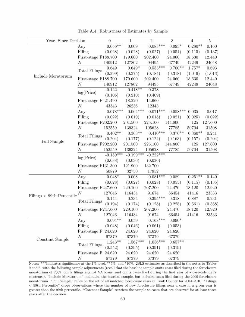
Table A.4: Robustness of Estimates by Sample

Years Since Decision 0 1 2 3 4 5Any 0.056** 0.009 0.083*** 0.093* 0.280** 0.160

Include Moratorium

Filing (0.028) (0.028) (0.027) (0.054) (0.115) (0.137)First-stage F188.700 179.600 202.400 24.060 18.630 12.440N 140912 127802 94495 67749 42249 24048

Total Filings 0.649 0.649* 0.553*** 0.700** 1.757* 0.693(0.399) (0.375) (0.184) (0.318) (1.019) (1.013)

First-stage F188.700 179.600 202.400 24.060 18.630 12.440N 140912 127802 94495 67749 42249 24048

log(Price) -0.122 -0.418** -0.378(0.106) (0.210) (0.409)

First-stage F 21.490 18.220 14.660N 43343 26236 12343Any 0.078*** 0.064*** 0.071*** 0.058*** 0.035 0.017

Full Sample

Filing (0.022) (0.019) (0.018) (0.021) (0.025) (0.022)First-stage F202.200 201.500 225.100 144.800 125 127.600N 152559 139324 105628 77785 50704 31508

Total Filings 0.402** 0.363** 0.410*** 0.376** 0.360** 0.241(0.204) (0.177) (0.124) (0.163) (0.157) (0.204)

First-stage F202.200 201.500 225.100 144.800 125 127.600N 152559 139324 105628 77785 50704 31508

log(Price) -0.159*** -0.199*** -0.222***(0.038) (0.036) (0.036)

First-stage F131.300 121.900 132.700N 50879 32750 17952Any 0.048* 0.008 0.081*** 0.089 0.251** 0.140

Filings < 99th Percentile

Filing (0.028) (0.027) (0.028) (0.055) (0.115) (0.135)First-stage F247.600 229.100 207.200 24.470 18.120 12.920N 127046 116434 91674 66454 41416 23533

Total Filings 0.144 0.234 0.395*** 0.318 0.887 0.231(0.194) (0.174) (0.128) (0.225) (0.561) (0.568)

First-stage F247.600 229.100 207.200 24.470 18.120 12.920N 127046 116434 91674 66454 41416 23533Any 0.094** 0.059 0.168*** 0.090*

Constant Sample

Filing (0.048) (0.046) (0.061) (0.053)First-stage F 24.620 24.620 24.620 24.620N 67379 67379 67379 67379

Total Filings 1.243** 1.567*** 1.056*** 0.657**(0.552) (0.395) (0.391) (0.319)

First-stage F 24.620 24.620 24.620 24.620N 67379 67379 67379 67379

Notes: ***Indicates significance at the 1% level, **5%, and *10%. 2SLS estimates as described in the notes to Tables9 and 6, with the following sample adjustments (recall that the baseline sample omits cases filed during the foreclosuremoratorium of 2009, omits filings against VA loans, and omits cases filed during the first year of a case-calendar’sexistence). “Include Moratorium” maintains the baseline sample, but includes cases filed during the 2009 foreclosuremoratorium. “Full Sample” relies on the set of all matched foreclosure cases in Cook County for 2004–2010. “Filings< 99th Percentile” drops observations where the number of new foreclosure filings near a case in a given year isgreater than the 99th percentile. “Constant Sample” restricts the sample to cases that are observed for at least threeyears after the decision.

60

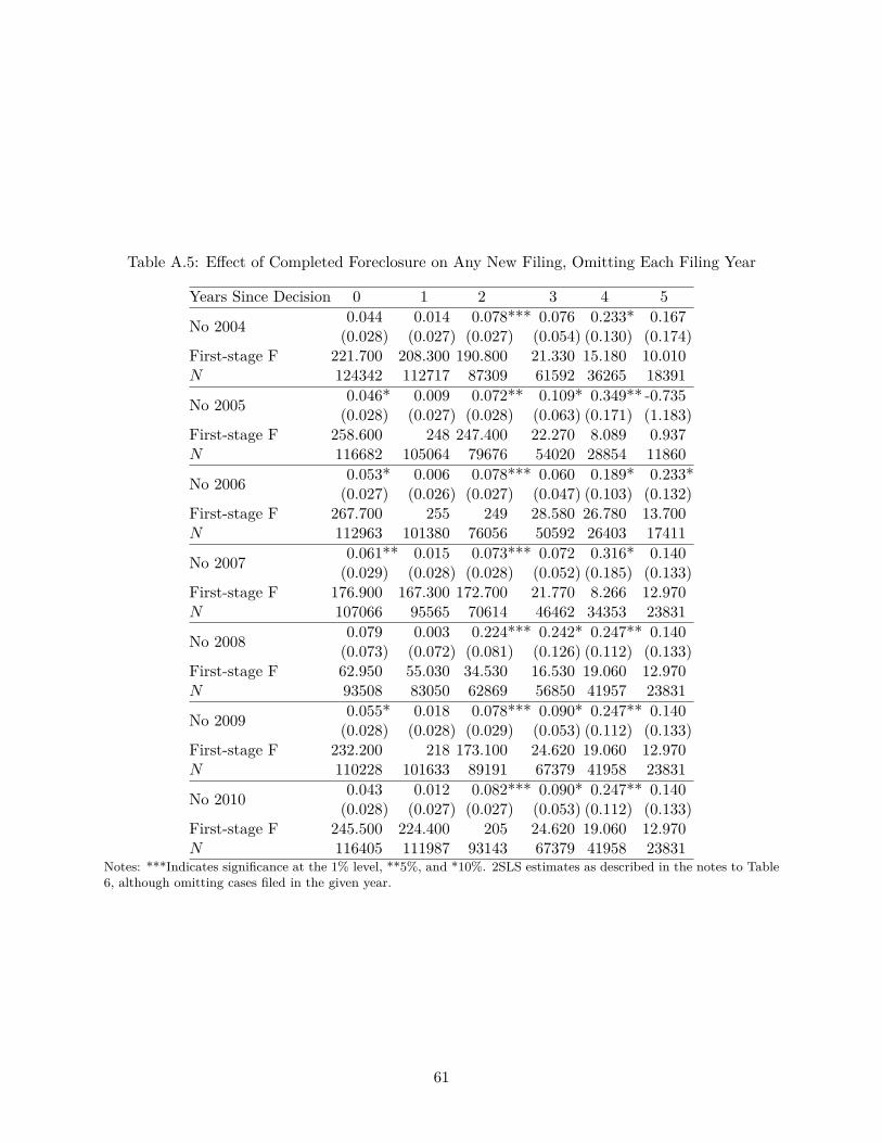
Table A.5: Effect of Completed Foreclosure on Any New Filing, Omitting Each Filing Year

Years Since Decision 0 1 2 3 4 5

No 2004 0.044 0.014 0.078*** 0.076 0.233* 0.167(0.028) (0.027) (0.027) (0.054) (0.130) (0.174)

First-stage F 221.700 208.300 190.800 21.330 15.180 10.010N 124342 112717 87309 61592 36265 18391

No 2005 0.046* 0.009 0.072** 0.109* 0.349** -0.735(0.028) (0.027) (0.028) (0.063) (0.171) (1.183)

First-stage F 258.600 248 247.400 22.270 8.089 0.937N 116682 105064 79676 54020 28854 11860

No 2006 0.053* 0.006 0.078*** 0.060 0.189* 0.233*(0.027) (0.026) (0.027) (0.047) (0.103) (0.132)

First-stage F 267.700 255 249 28.580 26.780 13.700N 112963 101380 76056 50592 26403 17411

No 2007 0.061** 0.015 0.073*** 0.072 0.316* 0.140(0.029) (0.028) (0.028) (0.052) (0.185) (0.133)

First-stage F 176.900 167.300 172.700 21.770 8.266 12.970N 107066 95565 70614 46462 34353 23831

No 2008 0.079 0.003 0.224*** 0.242* 0.247** 0.140(0.073) (0.072) (0.081) (0.126) (0.112) (0.133)

First-stage F 62.950 55.030 34.530 16.530 19.060 12.970N 93508 83050 62869 56850 41957 23831

No 2009 0.055* 0.018 0.078*** 0.090* 0.247** 0.140(0.028) (0.028) (0.029) (0.053) (0.112) (0.133)

First-stage F 232.200 218 173.100 24.620 19.060 12.970N 110228 101633 89191 67379 41958 23831

No 2010 0.043 0.012 0.082*** 0.090* 0.247** 0.140(0.028) (0.027) (0.027) (0.053) (0.112) (0.133)

First-stage F 245.500 224.400 205 24.620 19.060 12.970N 116405 111987 93143 67379 41958 23831

Notes: ***Indicates significance at the 1% level, **5%, and *10%. 2SLS estimates as described in the notes to Table6, although omitting cases filed in the given year.

61

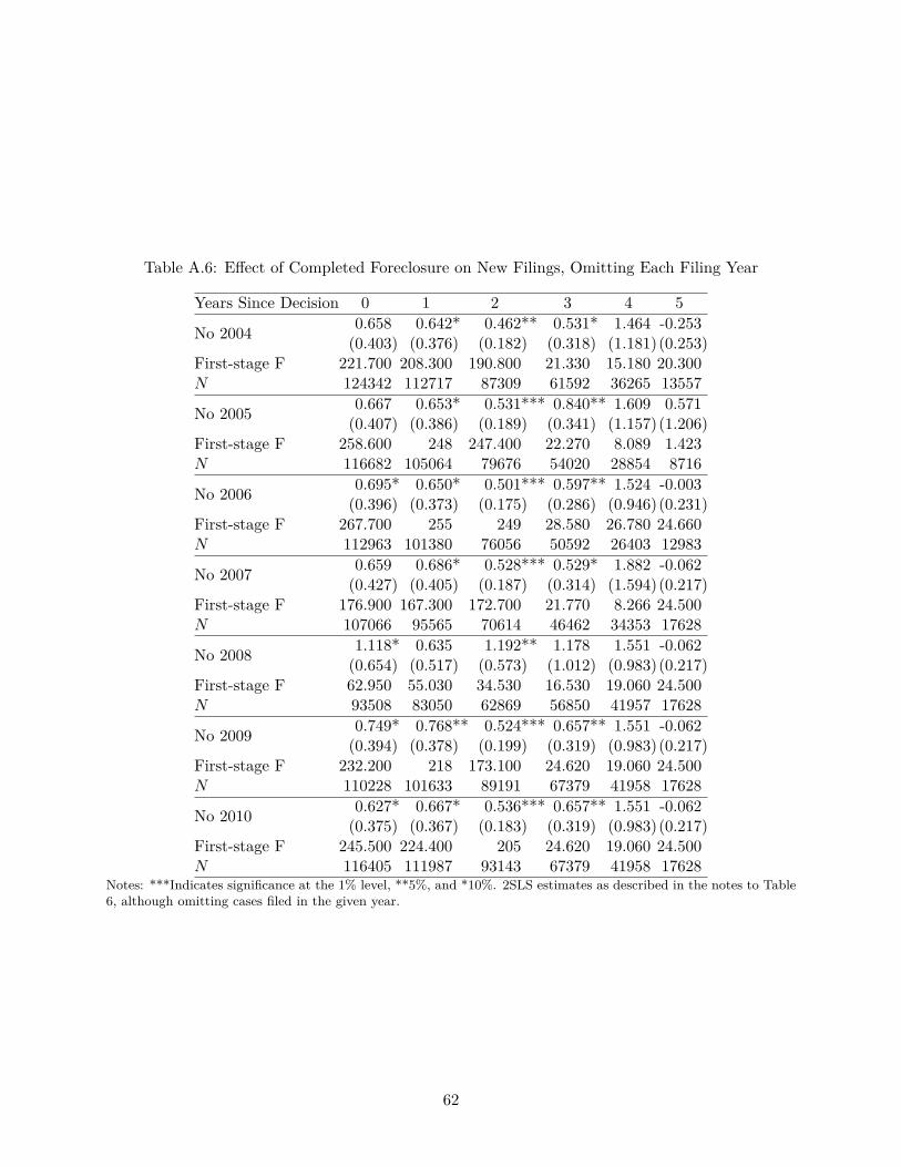
Table A.6: Effect of Completed Foreclosure on New Filings, Omitting Each Filing Year

Years Since Decision 0 1 2 3 4 5

No 2004 0.658 0.642* 0.462** 0.531* 1.464 -0.253(0.403) (0.376) (0.182) (0.318) (1.181)(0.253)

First-stage F 221.700 208.300 190.800 21.330 15.180 20.300N 124342 112717 87309 61592 36265 13557

No 2005 0.667 0.653* 0.531*** 0.840** 1.609 0.571(0.407) (0.386) (0.189) (0.341) (1.157)(1.206)

First-stage F 258.600 248 247.400 22.270 8.089 1.423N 116682 105064 79676 54020 28854 8716

No 2006 0.695* 0.650* 0.501*** 0.597** 1.524 -0.003(0.396) (0.373) (0.175) (0.286) (0.946)(0.231)

First-stage F 267.700 255 249 28.580 26.780 24.660N 112963 101380 76056 50592 26403 12983

No 2007 0.659 0.686* 0.528*** 0.529* 1.882 -0.062(0.427) (0.405) (0.187) (0.314) (1.594)(0.217)

First-stage F 176.900 167.300 172.700 21.770 8.266 24.500N 107066 95565 70614 46462 34353 17628

No 2008 1.118* 0.635 1.192** 1.178 1.551 -0.062(0.654) (0.517) (0.573) (1.012) (0.983)(0.217)

First-stage F 62.950 55.030 34.530 16.530 19.060 24.500N 93508 83050 62869 56850 41957 17628

No 2009 0.749* 0.768** 0.524*** 0.657** 1.551 -0.062(0.394) (0.378) (0.199) (0.319) (0.983)(0.217)

First-stage F 232.200 218 173.100 24.620 19.060 24.500N 110228 101633 89191 67379 41958 17628

No 2010 0.627* 0.667* 0.536*** 0.657** 1.551 -0.062(0.375) (0.367) (0.183) (0.319) (0.983)(0.217)

First-stage F 245.500 224.400 205 24.620 19.060 24.500N 116405 111987 93143 67379 41958 17628

Notes: ***Indicates significance at the 1% level, **5%, and *10%. 2SLS estimates as described in the notes to Table6, although omitting cases filed in the given year.

62

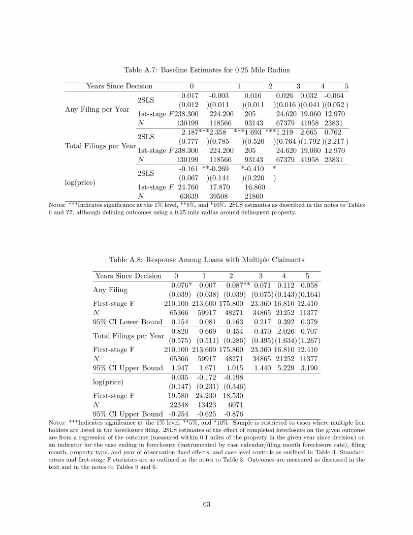
Table A.7: Baseline Estimates for 0.25 Mile Radius

Years Since Decision 0 1 2 3 4 5

Any Filing per Year2SLS 0.017 -0.003 0.016 0.026 0.032 -0.064

(0.012 )(0.011 )(0.011 )(0.016 )(0.041 )(0.052 )1st-stage F238.300 224.200 205 24.620 19.060 12.970N 130199 118566 93143 67379 41958 23831

Total Filings per Year2SLS 2.187***2.358 ***1.693 ***1.219 2.665 0.762

(0.777 )(0.785 )(0.520 )(0.764 )(1.792 )(2.217 )1st-stage F238.300 224.200 205 24.620 19.060 12.970N 130199 118566 93143 67379 41958 23831

log(price)2SLS -0.161 **-0.269 *-0.410 *

(0.067 )(0.144 )(0.220 )1st-stage F 24.760 17.870 16.860N 63639 39508 21860

Notes: ***Indicates significance at the 1% level, **5%, and *10%. 2SLS estimates as described in the notes to Tables6 and ??, although defining outcomes using a 0.25 mile radius around delinquent property.

Table A.8: Response Among Loans with Multiple Claimants

Years Since Decision 0 1 2 3 4 5

Any Filing 0.076* 0.007 0.087** 0.071 0.112 0.058(0.039) (0.038) (0.039) (0.075)(0.143)(0.164)

First-stage F 210.100 213.600 175.800 23.360 16.810 12.410N 65366 59917 48271 34865 21252 1137795% CI Lower Bound 0.154 0.081 0.163 0.217 0.392 0.379

Total Filings per Year 0.820 0.669 0.454 0.470 2.026 0.707(0.575) (0.511) (0.286) (0.495)(1.634)(1.267)

First-stage F 210.100 213.600 175.800 23.360 16.810 12.410N 65366 59917 48271 34865 21252 1137795% CI Upper Bound 1.947 1.671 1.015 1.440 5.229 3.190

log(price) 0.035 -0.172 -0.198(0.147) (0.231) (0.346)

First-stage F 19.580 24.230 18.530N 22348 13423 607195% CI Upper Bound -0.254 -0.625 -0.876

Notes: ***Indicates significance at the 1% level, **5%, and *10%. Sample is restricted to cases where multiple lienholders are listed in the foreclosure filing. 2SLS estimates of the effect of completed foreclosure on the given outcomeare from a regression of the outcome (measured within 0.1 miles of the property in the given year since decision) onan indicator for the case ending in foreclosure (instrumented by case calendar/filing month foreclosure rate), filingmonth, property type, and year of observation fixed effects, and case-level controls as outlined in Table 3. Standarderrors and first-stage F statistics are as outlined in the notes to Table 3. Outcomes are measured as discussed in thetext and in the notes to Tables 9 and 6.

63

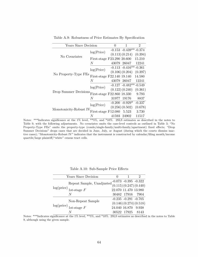
Table A.9: Robustness of Price Estimates By Specification

Years Since Decision 0 1 2

No Covariateslog(Price) -0.153 -0.439** -0.374

(0.113)(0.214) (0.394)First-stage F23.290 20.600 15.210N 43079 26047 12241

No Property-Type FEslog(Price) -0.113 -0.416** -0.361

(0.106)(0.204) (0.397)First-stage F22.140 19.140 14.580N 43079 26047 12241

Drop Summer Decisionslog(Price) -0.127 -0.482** -0.549

(0.122)(0.240) (0.361)First-stage F22.860 18.330 9.793N 31977 19176 8837

Monotonicity-Robust IVlog(Price) -0.200 -0.929* -0.337

(0.256)(0.502) (0.678)First-stage F12.080 5.523 3.730N 41593 24902 11517

Notes: ***Indicates significance at the 1% level, **5%, and *10%. 2SLS estimates as described in the notes toTable 9, with the following adjustments. No covariates omits the case-level controls as outlined in Table 3; “NoProperty-Type FEs” omits the property-type (condo/single-family/multi-family/apartment) fixed effects; “DropSummer Decisions” drops cases that are decided in June, July, or August (during which the courts dismiss inac-tive cases); “Monotonicity-Robust IV” indicates that the instrument is constructed by calendar/filing month/incomequartile/large plaintiff/“white” census tract cells.

Table A.10: Sub-Sample Price Effects

Years Since Decision 0 1 2

Repeat Sample, Unadjusted -0.073 -0.395 -0.322

log(price) (0.115)(0.247)(0.440)1st-stage F 22.070 11.470 13.980N 30482 17916 7904

Non-Repeat Sample -0.235 -0.291 -0.705

log(price) (0.146)(0.274)(0.518)1st-stage F 24.040 16.870 9.938N 30522 17925 8143

Notes: ***Indicates significance at the 1% level, **5%, and *10%. 2SLS estimates as described in the notes to Table9, although using the given sample.

64

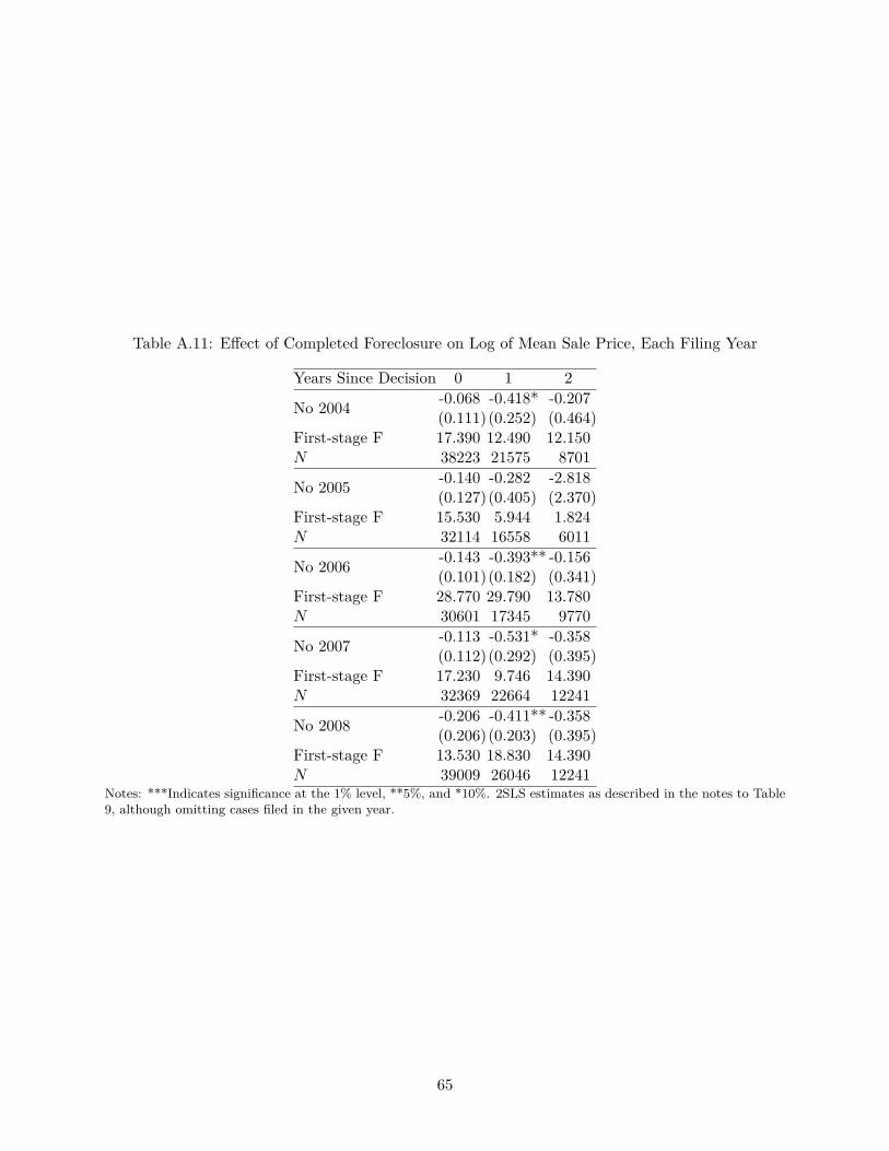
Table A.11: Effect of Completed Foreclosure on Log of Mean Sale Price, Each Filing Year

Years Since Decision 0 1 2

No 2004 -0.068 -0.418* -0.207(0.111)(0.252) (0.464)

First-stage F 17.390 12.490 12.150N 38223 21575 8701

No 2005 -0.140 -0.282 -2.818(0.127)(0.405) (2.370)

First-stage F 15.530 5.944 1.824N 32114 16558 6011

No 2006 -0.143 -0.393** -0.156(0.101)(0.182) (0.341)

First-stage F 28.770 29.790 13.780N 30601 17345 9770

No 2007 -0.113 -0.531* -0.358(0.112)(0.292) (0.395)

First-stage F 17.230 9.746 14.390N 32369 22664 12241

No 2008 -0.206 -0.411** -0.358(0.206)(0.203) (0.395)

First-stage F 13.530 18.830 14.390N 39009 26046 12241

Notes: ***Indicates significance at the 1% level, **5%, and *10%. 2SLS estimates as described in the notes to Table9, although omitting cases filed in the given year.

65

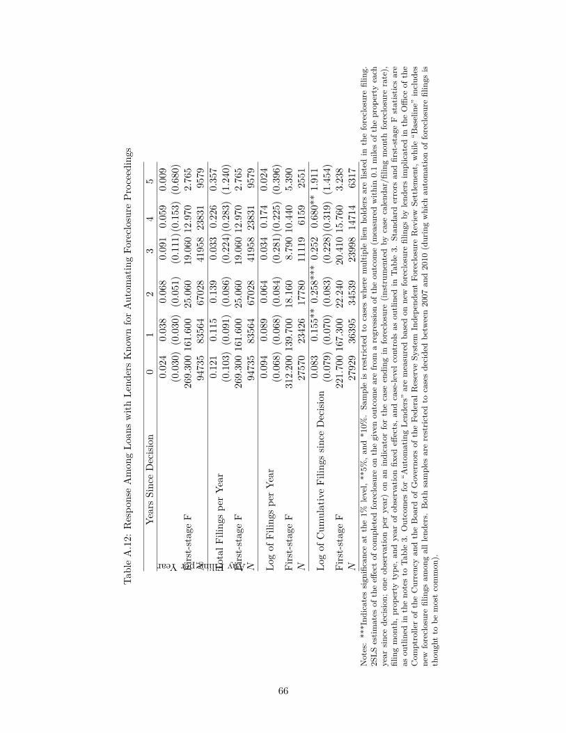
Tabl

eA

.12:

Res

pons

eA

mon

gLo

ans

with

Lend

ers

Kno

wn

for

Aut

omat

ing

Fore

clos

ure

Proc

eedi

ngs

Year

sSi

nce

Dec

ision

01

23

45

AnyFilingperYear0.

024

0.03

80.

068

0.09

10.

059

0.00

9(0

.030

)(0

.030

)(0

.051

)(0

.111

)(0.

153)

(0.6

80)

Firs

t-st

age

F26

9.30

016

1.60

025

.060

19.0

6012

.970

2.76

5N

9473

583

564

6702

841

958

2383

195

79

Tota

lFili

ngs

per

Year

0.12

10.

115

0.13

90.

033

0.22

60.

357

(0.1

03)

(0.0

91)

(0.0

86)

(0.2

24)(

0.28

3)(1

.240

)Fi

rst-

stag

eF

269.

300

161.

600

25.0

6019

.060

12.9

702.

765

N94

735

8356

467

028

4195

823

831

9579

Log

ofFi

lings

per

Year

0.09

40.

089

0.06

40.

034

0.17

40.

024

(0.0

68)

(0.0

68)

(0.0

84)

(0.2

81)(

0.22

5)(0

.396

)Fi

rst-

stag

eF

312.

200

139.

700

18.1

608.

790

10.4

405.

390

N27

570

2342

617

780

1111

961

5925

51

Log

ofC

umul

ativ

eFi

lings

since

Dec

ision

0.08

30.

155*

*0.

258*

**0.

252

0.68

0**

1.91

1(0

.079

)(0

.070

)(0

.083

)(0

.228

)(0.

319)

(1.4

54)

Firs

t-st

age

F22

1.70

016

7.30

022

.240

20.4

1015

.760

3.23

8N

2792

936

395

3453

923

998

1471

463

17N

otes

:**

*Ind

icat

essig

nific

ance

atth

e1%

leve

l,**

5%,a

nd*1

0%.

Sam

ple

isre

stric

ted

toca

ses

whe

rem

ultip

lelie

nho

lder

sar

elis

ted

inth

efo

recl

osur

efil

ing.

2SLS

estim

ates

ofth

eeff

ect

ofco

mpl

eted

fore

clos

ure

onth

egi

ven

outc

ome

are

from

are

gres

sion

ofth

eou

tcom

e(m

easu

red

with

in0.

1m

iles

ofth

epr

oper

tyea

chye

arsin

cede

cisio

n;on

eob

serv

atio

npe

rye

ar)

onan

indi

cato

rfo

rth

eca

seen

ding

info

recl

osur

e(in

stru

men

ted

byca

seca

lend

ar/fi

ling

mon

thfo

recl

osur

era

te),

filin

gm

onth

,pro

pert

yty

pe,a

ndye

arof

obse

rvat

ion

fixed

effec

ts,a

ndca

se-le

velc

ontr

ols

asou

tline

din

Tabl

e3.

Stan

dard

erro

rsan

dfir

st-s

tage

Fst

atist

ics

are

asou

tline

din

the

note

sto

Tabl

e3.

Out

com

esfo

r“A

utom

atin

gLe

nder

s”ar

em

easu

red

base

don

new

fore

clos

ure

filin

gsby

lend

ers

impl

icat

edin

the

Offi

ceof

the

Com

ptro

ller

ofth

eC

urre

ncy

and

the

Boa

rdof

Gov

erno

rsof

the

Fede

ralR

eser

veSy

stem

Inde

pend

ent

Fore

clos

ure

Rev

iew

Sett

lem

ent,

whi

le“B

asel

ine”

incl

udes

new

fore

clos

ure

filin

gsam

ong

alll

ende

rs.

Bot

hsa

mpl

esar

ere

stric

ted

toca

ses

deci

ded

betw

een

2007

and

2010

(dur

ing

whi

chau

tom

atio

nof

fore

clos

ure

filin

gsis

thou

ght

tobe

mos

tco

mm

on).

66

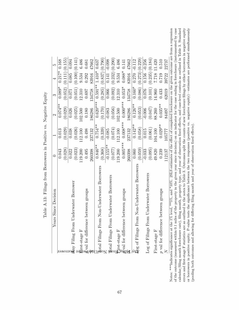
Tabl

eA

.13:

Filin

gsfro

mB

orro

wers

inPo

sitiv

evs

.N

egat

ive

Equi

ty

Year

sSi

nce

Dec

ision

01

23

45

AnyFilingFromNon-UnderwaterBorrower0.

043

0.01

30.

074*

*0.

089*

0.21

7*0.

168

(0.0

28)

(0.0

29)

(0.0

29)

(0.0

52)

(0.1

11)(

0.15

5)

Any

Filin

gFr

omU

nder

wate

rB

orro

wer

0.02

20.

038

0.02

60.

071

0.08

50.

094

(0.0

23)

(0.0

26)

(0.0

25)

(0.0

51)

(0.1

00)(

0.14

1)Fi

rst-

stag

eF

119.

200

112.

100

102.

500

12.3

109.

534

6.48

6p

valf

ordi

ffere

nce

betw

een

grou

ps0.

495

0.49

80.

180

0.69

70.

292

0.68

1N

2603

9823

7132

1862

8613

4758

8391

647

662

Tota

lFili

ngs

From

Non

-Und

erwa

ter

Bor

rowe

rs0.

846*

*0.

754*

*0.

620*

**0.

591*

*1.

410*

0.63

7(0

.368

)(0

.339

)(0

.170

)(0

.285

)(0

.837

)(0.

790)

Tota

lFili

ngs

From

Und

erwa

ter

Bor

rowe

rs-0

.155

**-0

.085

-0.0

830.

066

0.14

1-0

.098

(0.0

77)

(0.0

74)

(0.0

56)

(0.0

92)

(0.2

32)(

0.29

0)Fi

rst-

stag

eF

119.

200

112.

100

102.

500

12.3

109.

534

6.48

6p

valf

ordi

ffere

nce

betw

een

grou

ps0.

005*

**0.

008*

**0.

000*

**0.

053*

0.08

8*0.

141

N26

0398

2371

3218

6286

1347

5883

916

4766

2

Log

ofFi

lings

From

Non

-Und

erwa

ter

Bor

rowe

rs0.

060

0.14

2**

0.12

6**

0.16

0*0.

270

-0.1

12(0

.059

)(0

.058

)(0

.053

)(0

.086

)(0

.273

)(0.

229)

Log

ofFi

lings

From

Und

erwa

ter

Bor

rowe

rs-0

.033

0.01

5-0

.006

0.07

60.

156

-0.2

56(0

.095

)(0

.061

)(0

.047

)(0

.101

)(0

.235

)(0.

184)

Firs

t-st

age

F49

.820

104.

100

88.2

6014

.960

7.71

811

.420

pva

lfor

diffe

renc

ebe

twee

ngr

oups

0.23

90.

029*

*0.

035*

*0.

433

0.71

90.

510

N11

2137

1057

7784

497

6201

939

722

2273

7N

otes

:**

*Ind

icat

essig

nific

ance

atth

e1%

leve

l,**

5%,a

nd*1

0%.

2SLS

estim

ates

ofth

eeff

ecto

fcom

plet

edfo

recl

osur

eon

the

give

nou

tcom

ear

efr

oma

regr

essio

nof

the

outc

ome

(mea

sure

dw

ithin

0.1

mile

soft

hepr

oper

tyin

the

give

nye

arsin

cede

cisio

n)on

anin

dica

torf

orth

eca

seen

ding

info

recl

osur

e(in

stru

men

ted

byca

seca

lend

ar/fi

ling

mon

thfo

recl

osur

era

te),

filin

gm

onth

,pro

pert

yty

pe,a

ndye

arof

obse

rvat

ion

fixed

effec

ts,a

ndca

se-le

velc

ontr

ols

asou

tline

din

Tabl

e3.

Stan

dard

erro

rsan

dfir

st-s

tage

Fst

atist

icsa

reas

outli

ned

inth

eno

test

oTa

ble

3.O

utco

mes

split

the

coun

tsof

new

fore

clos

ure

filin

gsby

eith

erbo

rrow

ersi

nne

gativ

eeq

uity

orbo

rrow

ers

inpo

sitiv

eeq

uity

.P-

valu

ete

sts

the

signi

fican

cebe

twee

nth

etw

ore

spon

ses

(pos

itive

vs.

nega

tive

equi

ty)—

estim

ates

are

perf

orm

edsim

ulta

neou

sly(p

oolin

gbo

thou

tcom

esan

dal

low

ing

for

diffe

ring

filin

gm

onth

and

year

ofob

serv

atio

nfix

edeff

ects

).

67

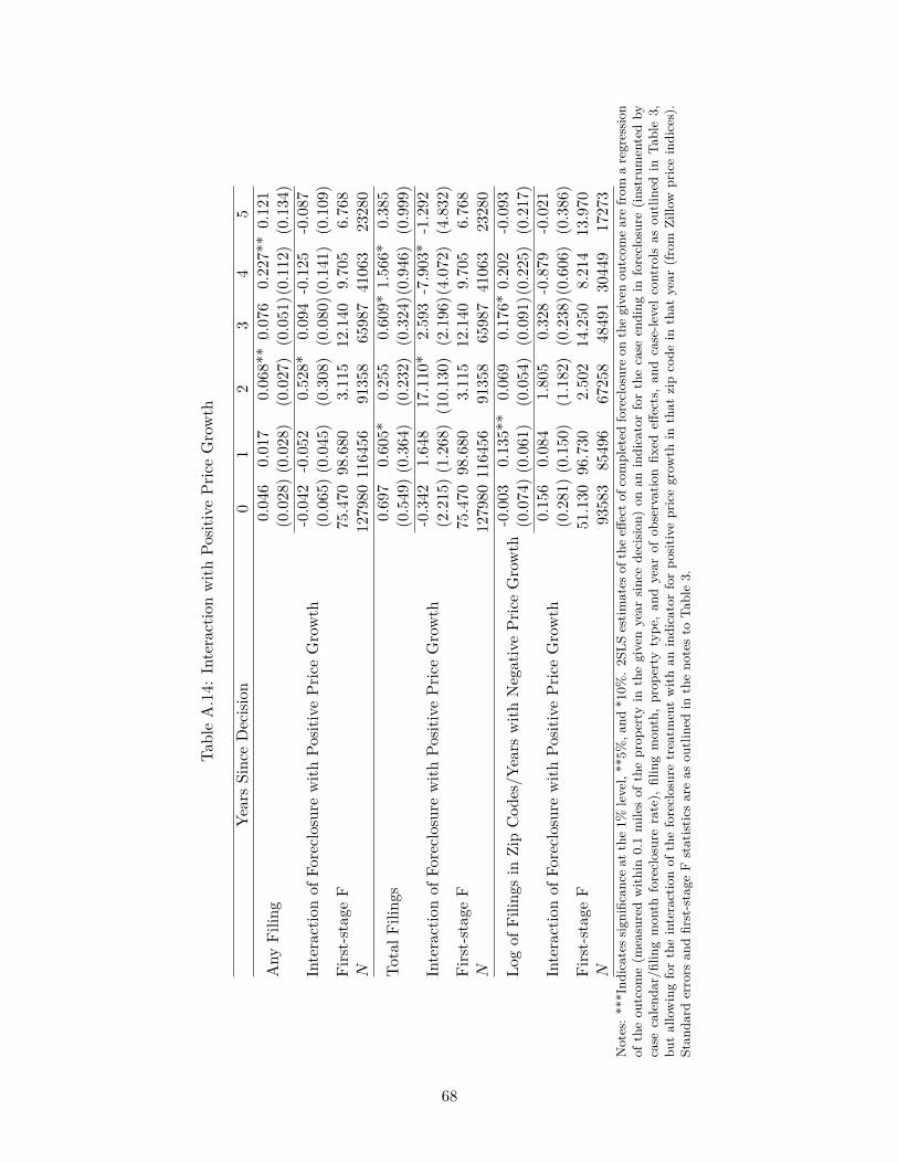
Tabl

eA

.14:

Inte

ract

ion

with

Posit

ive

Pric

eG

row

th

Year

sSi

nce

Dec

ision

01

23

45

Any

Filin

g0.

046

0.01

70.

068*

*0.

076

0.22

7**

0.12

1(0

.028

)(0

.028

)(0

.027

)(0

.051

)(0.

112)

(0.1

34)

Inte

ract

ion

ofFo

recl

osur

ew

ithPo

sitiv

ePr

ice

Gro

wth

-0.0

42-0

.052

0.52

8*0.

094

-0.1

25-0

.087

(0.0

65)

(0.0

45)

(0.3

08)

(0.0

80)(

0.14

1)(0

.109

)Fi

rst-

stag

eF

75.4

7098

.680

3.11

512

.140

9.70

56.

768

N12

7980

1164

5691

358

6598

741

063

2328

0

Tota

lFili

ngs

0.69

70.

605*

0.25

50.

609*

1.56

6*0.

385

(0.5

49)

(0.3

64)

(0.2

32)

(0.3

24)(

0.94

6)(0

.999

)

Inte

ract

ion

ofFo

recl

osur

ew

ithPo

sitiv

ePr

ice

Gro

wth

-0.3

421.

648

17.1

10*

2.59

3-7

.903

*-1

.292

(2.2

15)

(1.2

68)

(10.

130)

(2.1

96)(

4.07

2)(4

.832

)Fi

rst-

stag

eF

75.4

7098

.680

3.11

512

.140

9.70

56.

768

N12

7980

1164

5691

358

6598

741

063

2328

0

Log

ofFi

lings

inZi

pC

odes

/Yea

rsw

ithN

egat

ive

Pric

eG

row

th-0

.003

0.13

5**

0.06

90.

176*

0.20

2-0

.093

(0.0

74)

(0.0

61)

(0.0

54)

(0.0

91)(

0.22

5)(0

.217

)

Inte

ract

ion

ofFo

recl

osur

ew

ithPo

sitiv

ePr

ice

Gro

wth

0.15

60.

084

1.80

50.

328

-0.8

79-0

.021

(0.2

81)

(0.1

50)

(1.1

82)

(0.2

38)(

0.60

6)(0

.386

)Fi

rst-

stag

eF

51.1

3096

.730

2.50

214

.250

8.21

413

.970

N93

583

8549

667

258

4849

130

449

1727

3N

otes

:**

*Ind

icat

essig

nific

ance

atth

e1%

leve

l,**

5%,a

nd*1

0%.

2SLS

estim

ates

ofth

eeff

ecto

fcom

plet

edfo

recl

osur

eon

the

give

nou

tcom

ear

efr

oma

regr

essio

nof

the

outc

ome

(mea

sure

dw

ithin

0.1

mile

sof

the

prop

erty

inth

egi

ven

year

since

deci

sion)

onan

indi

cato

rfo

rth

eca

seen

ding

info

recl

osur

e(in

stru

men

ted

byca

seca

lend

ar/fi

ling

mon

thfo

recl

osur

era

te),

filin

gm

onth

,pr

oper

tyty

pe,

and

year

ofob

serv

atio

nfix

edeff

ects

,an

dca

se-le

vel

cont

rols

asou

tline

din

Tabl

e3,

but

allo

win

gfo

rth

ein

tera

ctio

nof

the

fore

clos

ure

trea

tmen

tw

ithan

indi

cato

rfo

rpo

sitiv

epr

ice

grow

thin

that

zip

code

inth

atye

ar(f

rom

Zillo

wpr

ice

indi

ces)

.St

anda

rder

rors

and

first

-sta

geF

stat

istic

sar

eas

outli

ned

inth

eno

tes

toTa

ble

3.

68

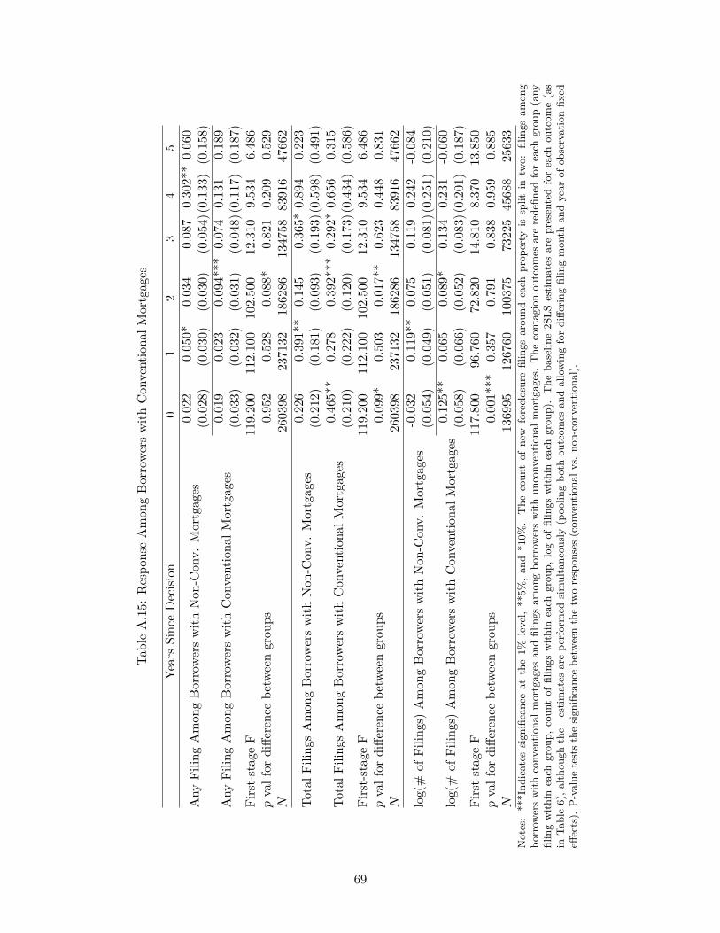
Tabl

eA

.15:

Res

pons

eA

mon

gB

orro

wers

with

Con

vent

iona

lMor

tgag

es

Year

sSi

nce

Dec

ision

01

23

45

Any

Filin

gA

mon

gB

orro

wers

with

Non

-Con

v.M

ortg

ages

0.02

20.

050*

0.03

40.

087

0.30

2**

0.06

0(0

.028

)(0

.030

)(0

.030

)(0

.054

)(0.

133)

(0.1

58)

Any

Filin

gA

mon

gB

orro

wers

with

Con

vent

iona

lMor

tgag

es0.

019

0.02

30.

094*

**0.

074

0.13

10.

189

(0.0

33)

(0.0

32)

(0.0

31)

(0.0

48)(

0.11

7)(0

.187

)Fi

rst-

stag

eF

119.

200

112.

100

102.

500

12.3

109.

534

6.48

6p

valf

ordi

ffere

nce

betw

een

grou

ps0.

952

0.52

80.

088*

0.82

10.

209

0.52

9N

2603

9823

7132

1862

8613

4758

8391

647

662

Tota

lFili

ngs

Am

ong

Bor

rowe

rsw

ithN

on-C

onv.

Mor

tgag

es0.

226

0.39

1**

0.14

50.

365*

0.89

40.

223

(0.2

12)

(0.1

81)

(0.0

93)

(0.1

93)(

0.59

8)(0

.491

)

Tota

lFili

ngs

Am

ong

Bor

rowe

rsw

ithC

onve

ntio

nalM

ortg

ages

0.46

5**

0.27

80.

392*

**0.

292*

0.65

60.

315

(0.2

10)

(0.2

22)

(0.1

20)

(0.1

73)(

0.43

4)(0

.586

)Fi

rst-

stag

eF

119.

200

112.

100

102.

500

12.3

109.

534

6.48

6p

valf

ordi

ffere

nce

betw

een

grou

ps0.

099*

0.50

30.

017*

*0.

623

0.44

80.

831

N26

0398

2371

3218

6286

1347

5883

916

4766

2

log(

#of

Filin

gs)

Am

ong

Bor

rowe

rsw

ithN

on-C

onv.

Mor

tgag

es-0

.032

0.11

9**

0.07

50.

119

0.24

2-0

.084

(0.0

54)

(0.0

49)

(0.0

51)

(0.0

81)(

0.25

1)(0

.210

)

log(

#of

Filin

gs)

Am

ong

Bor

rowe

rsw

ithC

onve

ntio

nalM

ortg

ages

0.12

5**

0.06

50.

089*

0.13

40.

231

-0.0

60(0

.058

)(0

.066

)(0

.052

)(0

.083

)(0.

201)

(0.1

87)

Firs

t-st

age

F11

7.80

096

.760

72.8

2014

.810

8.37

013

.850

pva

lfor

diffe

renc

ebe

twee

ngr

oups

0.00

1***

0.35

70.

791

0.83

80.

959

0.88

5N

1369

9512

6760

1003

7573

225

4568

825

633

Not

es:

***I

ndic

ates

signi

fican

ceat

the

1%le

vel,

**5%

,an

d*1

0%.

The

coun

tof

new

fore

clos

ure

filin

gsar

ound

each

prop

erty

issp

litin

two:

filin

gsam

ong

borr

ower

sw

ithco

nven

tiona

lmor

tgag

esan

dfil

ings

amon

gbo

rrow

ers

with

unco

nven

tiona

lmor

tgag

es.

The

cont

agio

nou

tcom

esar

ere

defin

edfo

rea

chgr

oup

(any

filin

gw

ithin

each

grou

p,co

unt

offil

ings

with

inea

chgr

oup,

log

offil

ings

with

inea

chgr

oup)

.T

heba

selin

e2S

LSes

timat

esar

epr

esen

ted

for

each

outc

ome

(as

inTa

ble

6),a

lthou

ghth

e—es

timat

esar

epe

rfor

med

simul

tane

ously

(poo

ling

both

outc

omes

and

allo

win

gfo

rdi

fferin

gfil

ing

mon

than

dye

arof

obse

rvat

ion

fixed

effec

ts).

P-va

lue

test

sth

esig

nific

ance

betw

een

the

two

resp

onse

s(c

onve

ntio

nalv

s.no

n-co

nven

tiona

l).

69

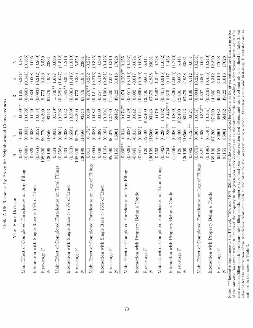
Tabl

eA

.16:

Res

pons

eby

Prox

yfo

rN

eigh

borh

ood

Con

nect

edne

ss

Year

sSi

nce

Dec

ision

01

23

45

Mai

nEff

ect

ofC

ompl

eted

Fore

clos

ure

onA

nyFi

ling

0.03

70.

031

0.09

0**

0.10

50.

241*

0.18

5(0

.040

)(0

.038

)(0

.038

)(0

.066

)(0

.141

)(0

.185

)

Inte

ract

ion

with

Sing

leR

ace

>75

%of

Trac

t0.

025

-0.0

38-0

.020

-0.0

34-0

.008

-0.0

95(0

.054

)(0

.052

)(0

.053

)(0

.093

)(0

.212

)(0

.260

)Fi

rst-

stag

eF

108.

600

99.7

7084

.300

9.77

39.

330

5.55

9N

1301

9911

8566

9314

367

379

4195

823

831

Mai

nEff

ect

ofC

ompl

eted

Fore

clos

ure

onTo

talF

iling

s0.

404

0.83

40.

570*

1.34

6**

1.67

7-0

.096

(0.5

58)

(0.6

62)

(0.2

96)

(0.5

29)

(1.0

47)

(1.5

12)

Inte

ract

ion

with

Sing

leR

ace

>75

%of

Trac

t0.

534

-0.3

38-0

.132

-1.3

85**

-0.3

941.

216

(0.8

13)

(0.6

50)

(0.3

69)

(0.6

30)

(1.4

16)

(1.8

10)

Firs

t-st

age

F10

8.60

099

.770

84.3

009.

773

9.33

05.

559

N13

0199

1185

6693

143

6737

941

958

2383

1

Mai

nEff

ect

ofC

ompl

eted

Fore

clos

ure

onLo

gof

Filin

gs0.

011

0.17

2*0.

090

0.27

6**

0.25

2-0

.277

(0.0

94)

(0.0

88)

(0.0

82)

(0.1

21)

(0.2

73)

(0.3

45)

Inte

ract

ion

with

Sing

leR

ace

>75

%of

Trac

t0.

009

-0.0

82-0

.009

-0.2

57-0

.119

0.38

0(0

.110

)(0

.108

)(0

.104

)(0

.166

)(0

.391

)(0

.423

)Fi

rst-

stag

eF

95.5

9096

.070

72.7

3011

.620

7.09

710

.310

N95

155

8696

168

482

4942

231

016

1762

8

Mai

nEff

ect

ofC

ompl

eted

Fore

clos

ure

onA

nyFi

ling

0.06

0**

0.01

40.

074*

*0.

074

0.25

0**

0.15

5(0

.029

)(0

.028

)(0

.029

)(0

.057

)(0

.116

)(0

.137

)

Inte

ract

ion

with

Prop

erty

Bei

nga

Con

do-0

.045

-0.0

130.

042

0.09

2-0

.017

-0.0

74(0

.041

)(0

.035

)(0

.044

)(0

.066

)(0

.109

)(0

.085

)Fi

rst-

stag

eF

120

112.

400

102.

400

12.4

009.

603

6.41

4N

1301

9911

8566

9314

367

379

4195

823

831

Mai

nEff

ect

ofC

ompl

eted

Fore

clos

ure

onTo

talF

iling

s0.

563

0.26

10.

079

0.54

9*1.

529*

0.24

8(0

.392

)(0

.296

)(0

.192

)(0

.331

)(0

.916

)(1

.032

)

Inte

ract

ion

with

Prop

erty

Bei

nga

Con

do0.

704

2.23

6**

2.44

6***

0.61

50.

117

1.45

3(1

.656

)(0

.986

)(0

.869

)(1

.326

)(2

.005

)(1

.776

)Fi

rst-

stag

eF

120

112.

400

102.

400

12.4

009.

603

6.41

4N

1301

9911

8566

9314

367

379

4195

823

831

0.08

20.

125*

*0.

024

0.10

60.

112

-0.0

51

Mai

nEff

ect

ofC

ompl

eted

Fore

clos

ure

onLo

gof

Filin

gs(0

.075

)(0

.063

)(0

.057

)(0

.094

)(0

.227

)(0

.231

)-0

.321

0.03

60.

352*

*0.

307

0.50

1-0

.061

Inte

ract

ion

with

Prop

erty

Bei

nga

Con

do(0

.196

)(0

.146

)(0

.161

)(0

.219

)(0

.456

)(0

.240

)13

9.10

010

7.20

097

.200

14.6

608.

312

12.3

90Fi

rst-

stag

eF

9515

586

961

6848

249

422

3101

617

628

N95

155

8696

168

482

4942

231

016

1762

8N

otes

:**

*Ind

icat

essig

nific

ance

atth

e1%

leve

l,**

5%,a

nd*1

0%.

2SLS

estim

ates

ofth

eeff

ecto

fcom

plet

edfo

recl

osur

eon

the

give

nou

tcom

ear

efr

oma

regr

essio

nof

the

outc

ome

(mea

sure

dw

ithin

0.1

mile

sof

the

prop

erty

inth

egi

ven

year

since

deci

sion)

onan

indi

cato

rfo

rth

eca

seen

ding

info

recl

osur

e(in

stru

men

ted

byca

seca

lend

ar/fi

ling

mon

thfo

recl

osur

era

te),

filin

gm

onth

,pro

pert

yty

pe,a

ndye

arof

obse

rvat

ion

fixed

effec

ts,a

ndca

se-le

velc

ontr

ols

asou

tline

din

Tabl

e3,

but

allo

win

gfo

rth

ein

tera

ctio

nof

the

fore

clos

ure

trea

tmen

tw

ithan

indi

cato

rfo

rth

epr

oper

tybe

ing

aco

ndo.

Stan

dard

erro

rsan

dfir

st-s

tage

Fst

atist

ics

are

asou

tline

din

the

note

sto

Tabl

e3.

70

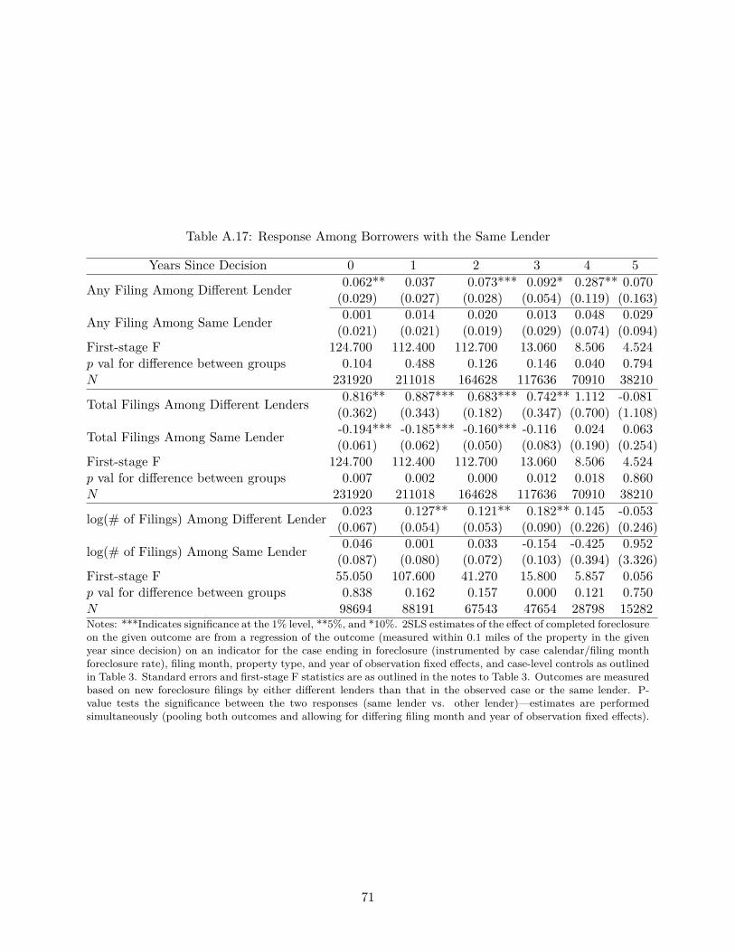
Table A.17: Response Among Borrowers with the Same Lender

Years Since Decision 0 1 2 3 4 5

Any Filing Among Different Lender 0.062** 0.037 0.073*** 0.092* 0.287** 0.070(0.029) (0.027) (0.028) (0.054) (0.119) (0.163)

Any Filing Among Same Lender 0.001 0.014 0.020 0.013 0.048 0.029(0.021) (0.021) (0.019) (0.029) (0.074) (0.094)

First-stage F 124.700 112.400 112.700 13.060 8.506 4.524p val for difference between groups 0.104 0.488 0.126 0.146 0.040 0.794N 231920 211018 164628 117636 70910 38210

Total Filings Among Different Lenders 0.816** 0.887*** 0.683*** 0.742** 1.112 -0.081(0.362) (0.343) (0.182) (0.347) (0.700) (1.108)

Total Filings Among Same Lender -0.194*** -0.185*** -0.160*** -0.116 0.024 0.063(0.061) (0.062) (0.050) (0.083) (0.190) (0.254)

First-stage F 124.700 112.400 112.700 13.060 8.506 4.524p val for difference between groups 0.007 0.002 0.000 0.012 0.018 0.860N 231920 211018 164628 117636 70910 38210

log(# of Filings) Among Different Lender 0.023 0.127** 0.121** 0.182** 0.145 -0.053(0.067) (0.054) (0.053) (0.090) (0.226) (0.246)

log(# of Filings) Among Same Lender 0.046 0.001 0.033 -0.154 -0.425 0.952(0.087) (0.080) (0.072) (0.103) (0.394) (3.326)

First-stage F 55.050 107.600 41.270 15.800 5.857 0.056p val for difference between groups 0.838 0.162 0.157 0.000 0.121 0.750N 98694 88191 67543 47654 28798 15282Notes: ***Indicates significance at the 1% level, **5%, and *10%. 2SLS estimates of the effect of completed foreclosureon the given outcome are from a regression of the outcome (measured within 0.1 miles of the property in the givenyear since decision) on an indicator for the case ending in foreclosure (instrumented by case calendar/filing monthforeclosure rate), filing month, property type, and year of observation fixed effects, and case-level controls as outlinedin Table 3. Standard errors and first-stage F statistics are as outlined in the notes to Table 3. Outcomes are measuredbased on new foreclosure filings by either different lenders than that in the observed case or the same lender. P-value tests the significance between the two responses (same lender vs. other lender)—estimates are performedsimultaneously (pooling both outcomes and allowing for differing filing month and year of observation fixed effects).

71