forecasting volatility in commodity markets

Journal of Forecasting, Vol. 14, 77-95 (1995)

Forecasting Volatility in Commodity Markets

KENNETH F. KRONER Department of Economics, University of Arizona and Advanced Strategies Research Group, Wells Fargo Nikko Investment Advisors

KEVIN P. KNEAFSEY Department of Finance, University of Arizona and Defined Contributions Group, Wells Fargo Nikko Investment Advisors

STIJN CLAESSENS World Bank

ABSTRACT This paper uses recent advances in time-series modelling to derive long- horizon forecasts of commodity price volatility which incorporate investors’ expectations of volatility. Our results are promising. We compare several different forecasts of commodity price volatility, which we divide into three categories: (1) forecasts using only expectations derived from options prices; (2) forecasts using only time-series modelling; and (3) forecasts which combine market expectations and time- series methods. The forecasts in (1) and (2) are used extensively in the literature, while those in (3) are new in this paper. On comparing these different forecasts, we find that our proposed forecasts from category (3) outperform both market expectations forecasts and time-series forecasts. This result holds both in and out of sample for virtually all commodities considered.

INTRODUCTION

Commodity prices have historically been one of the most volatile of international asset prices. Over the period 1972-90, for example, the volatility of non-oil commodity prices in nominal terms, as measured by the annualized standard deviation of percentage changes during the previous 24 months, has not been below 15%, and peaked at more than 50% in 1975. It is not surprising, then, that efforts to forecast commodity prices have been largely unsuccessful. In fact, it can be expected that ex-post forecast errors will continue to display a large distribution around zero, whether the forecasts are made using futures prices or specialists’ assessments. For this reason, it is useful to construct a measure of confidence in the price forecast. The traditional way to express confidence in a forecast is to bound it by a confidence interval, that is, to give an

Q 1995 by John Wiley & Sons, Ltd. Revised September 1994 CCC 0277 -6693/95/020077 - 19

78 Journal of Forecasting Vol. 14, Iss. No. 2

interval forecast and an associated probability. This is easily done in a world where volatility is constant, but if volatility is itself changing, then a forecast of volatility must be derived before an interval forecast can be constructed.

There are several reasons that such volatility forecasts of commodity prices are important. For example, the economies of many developing countries are tied tightly to the success of their principal commodity export. An assessment of the confidence in a commodity price forecast would therefore have policy implications for the governments of the developing countries. Second, commodity price volatility has implications for developed countries considering investing in and/or providing monetary aid to the developing countries, because theability of a developing country to repay the loan might be determined primarily by the wealth generated from commodity exports. The explosive growth in international investing, especially in developing countries, provides a third reason for the importance of volatility forecasts. This growth, which is evidenced by the increasing numbers of country funds and emerging market divisions in large brokerage houses, necessitates the use of long-horizon volatility forecasts as a means of evaluating forecasted economic development. Finally, volatility forecasts are crucial in the pricing of options contracts because, all else equal, a higher forecasted volatility should result in higher options prices. So if any investor has a better forecast of volatility than the market, he or she should be able to exploit the forecast to make excess returns.

The purpose of this paper is to develop methods of forecasting commodity price volatility over long time horizons, here taken as 225 calendar days. Several methods of forecasting volatility over short horizons already exist in the literature, but many of these methods are not appropriate for long-horizon forecasts. For example, implied standard deviation forecasts derived from options prices as in Latane and Rendelman (1976), Beckers (1983), Wei and Frankel (1991), and many others, may be appropriate for short-term forecasts, but are less reliable for long-term forecasts because trading is very thin in options that are far from their expiration dates. Also, traditional time-series methods, like ARMA models on moving standard deviations as in Cao and Tsay (1992), or ARMA models on bid-ask spreads or daily price ranges, as in Taylor (1987), are not likely to give useful forecasts because a 225-day forecast will generally be simply the unconditional mean of the series if volatility is mean reverting. To illustrate, the 225-day forecast from the ARMA(1, 1) model

Y r = w + ey+, + +&r- l + &,

is

which is approximately w/( l - 0) if I 61 c 1, i.e. if volatility is mean reverting. A similar result holds for the GARCH family of models. It is important to recognize that while volatility is probably mean reverting (Stein, 1989; Poterba and Summers, 1986), the literature indicates that the reversion occurs at a hyperbolic rate (Baillie et al., 1993; Bollerslev and Mikkelson, 1993), which is slower than ARMA and GAFCH models permit. This paper provides volatility forecasts for about 7; months, a period too long to apply conventional short-horizon forecasting methods, but too short to expect that the unconditional variance will best capture the dynamics of future volatility.

We will develop a forecasting model which combines investors' forecasts with time series

K . F. Kroner, K. P. Kneafsey and S . Claessens Forecasting Volatility 79

forecasts and produces forecasts of long-term volatility which are more accurate than the short- term forecasting methods. This result holds both in sample and out of sample for almost all the commodities we consider, suggesting that our proposed forecasting model can be an effective tool for constructing interval forecasts, and perhaps for pricing long-term options. The paper is organized as follows. The next section discusses some existing short-term volatility forecasting methods and the third section presents our new proposed forecasts. The fourth section discusses the data, the fifth section gives the results, and the final section presents conclusions.

EXISTING FORECASTS

Implied standard deviations One popular method of forecasting volatility uses option prices to measure investors’ expectations of future volatility. An option is a contract which permits, but does not require, the holder to buy (sell) the underlying asset at a predetermined price. Clearly, the more volatile the price of the underlying asset, the more likely it is that the option will have value, consequently the higher the option’s price. If the option market is efficient, then investors’ expectations of future volatility as embodied in option prices should be the best volatility forecast available. More specifically, option prices are functions of four observable variables (the price of the underlying asset, the exercise price of the option, the time to maturity of the option, and the risk-free rate of interest) and one unobservable variable (the expected volatility of returns on the u:derlying asset over the life of the optior.). Since the option price is itself observable, and since the option price is a monotonically increasing function of expected volatility, one can use an option pricing model to back out the market’s expectation of volatility over the remaining life of the option (Latane and Rendleman, 1976). This forecast of volatility is often called the implied standard deviation, or ISD. We refer to it as a ‘market-based’ forecast because it is based entirely on the expectations of participants in the options market (given a particular option pricing model).

To compute the ISD we require an option-pricing formula for commodity futures options. Most options on commodities are American options, meaning that they can be exercised either at any date on or before maturity or at any time within a specific period (e.g. one month) before maturity.’ This early exercise feature of commodity options means that they should sell at a premium relative to European options, which allow the option holder to exercise the option only on the maturity date of the option. This in turn means that the use of standard European option pricing formula of Black (1976) will result in ISDs which are overstated. The positive bias in the ISD occurs because the European formula assumes that the higher option price is due to higher volatility (and therefore a higher estimated ISD is obtained), when in reality the higher price might simply reflect the early exercise premium. Unfortunately, no closed-fonn solution exists for American options, though several approximation methods exist. We adopt the method of Barone-Adesi and Whaley (1987), who provide an efficient approximation for pricing American options on commodity futures. Their approximation relates the call price, C, to the futures price, F,, the time to expiration, T, the interest rate, r, the exercise price, X, and the

‘Early exercise is important when dealing with options on futures contracts. Ignoring storage costs and convenience yields, the futures price declines to the spot price as expiration nears. This makes the behaviour of futures prices similar to that of a stock price that pays out continuous dividends. These ‘implicit dividends’ can only be reaped if the option holder exercises his or her option.


volatility, u. See the Appendix for the details of their approximation.2 We will refer to the Barone-Adesi and Whaley (1987) price as C= C(F,, T , r, X , a).

Three important observations about the Barone-Adesi and Whaley (1987) pricing formula (see equation (A4) in the Appendix) merit mention. First, while it is mathematically complicated, it is easily programmed. Second, Barone-Adesi and Whaley (1987) show that their approximation becomes exact as the time to expiration gets large. In this paper we are focusing on long-horizon forecasts, so the approximation error should be quite small. Third, there are only six variables in this formula-C, X, F, r , T, and u. The first five are observable and therefore can be used to solve for u. This u, the ISD, is the measure of volatility implied by the option price, that is, the market's expectation of volatility over the remaining life of the contract.

In this paper we will evaluate a set of forecasts based on ISDs. But for any given day in our data set and for any given option maturity, there are several different options traded, one for each exercise price. For example, on 2 November 1988 there are twenty wheat contracts which expire in March 1989, each with a different strike price. Using these contracts separately, we can extract twenty different ISDs, or twenty different forecasts of volatility for the period November 1988 to March 1989.3 We used three different methods to collapse these multiple ISD forecasts into a single volatility forecast. The first takes the ISD from the contact for which the price of the option is most sensitive to changes in the volatility of the underlying commodity. Usually, this is the at-the-money option, but occasionally it is the near-the-money option4 This contract is used to extract the ISD for three reasons. First, because this contract price is the most sensitive to volatility, it should return the most accurate measure of volatility. Second, the value added by the American feature is the smallest for at-the-money options (Ramaswamy and Sundaresan, 1985). While we correct for the American feature, the correction is not perfect and we prefer to use the ISDs that are least influenced. Third, at-the-money options have the smallest bias when volatility is not constant. The Black model is (approximately) linear in volatility for at-the- money options, which implies that the at-the-money implied volatility estimates will result in only a small bias when volatility is stochastic (Hull and White, 1987).

Therefore one set of forecasts is the ISD extracted from the contract with the highest derivative of the call price with respect to volatility, in other words, the u which solves the equation

(1) where C'(t, T, X i ) is the observed call price at time t for a contract with time to expiration T and exercise price Xi, C(.) is the Barone-Adesi and Whaley (1987) formula given in equation (A4) in the Appendix, and i is chosen to maximize X/&. Throughout this paper, we refer to

C(F,, T , r . Xi. s ) - C'(t, T , Xi) = 0

'To demonstrate the potential magnitude of the bias from not accounting for the American feature of a commodity option, consider the May/1985 soybean future option selling on 2 November 1984 with an exercise price of $600. The futures price was $664.75, the spot price was $627.50, the call price was $76.00, and the annualized interest rate was 9.737%. Using Black's (1976) formula for pricing European futures options, the ISD is 0.2272, while using the Barone-Adesi and Whaley American option pricing approximation, the ISD is 0.2174. The overstatement using the European formula is thus about 5%.

All twenty of these forecasts do not return the same ISD. This is an indication of one or more of the following: the impact of price discreteness in an option pricing model that assumes continuous prices; misspecification in the option p m g model; and/or option market inefficiencies.

At-the-money' refers to the option whose exercise price is closest to the spot price of the underlying asset. The difference in the ISDs from the at-the-money option and the near-the-money option is l ie ly to be very small. To illustrate, in previous work by the authors using soybean data, the correlation between at-the-money ISDs and just-in- the-money ISDs from contracts with greater than 260 days to maturity is 0.9891.

K . F. Kroner, K. P. Kneafsey and S . Claessens Forecasting Volatility 81

this T-period forecast of volatility at time t as ISDAT,,T, for the ISD from the AT the money option.

Using ISDAT, however, ignores information about volatility that is available in other contracts. We therefore propose two other market-based forecasts of volatility which do not ignore the potentially useful information in the prices of options which are not at-the-money. First, we use a weighted average of all the ISDs that can be computed on a given date t for a given time to expiration T, with the weights being the derivatives of the option price with respect to volatility. More specifically, the forecast we use is

c Y7xj =mi

c Y7xi (2)

4 ISDAVG,,, =

xi

where omi is the ISD from a call option with T days to expiration and with exercise price X i , and yTxi is the derivative of the price of this call option with respect to volatility. This weighting mechanism was chosen because it places the most weight on the ISDs from options most sensitive to volatility changes. The idea is that more precise volatility estimates are returned by more sensitive options, and consequently the more sensitive options merit a higher weight. We call this forecast ISDAVG, because it is a weighted average of ISDs.

The second method we use to account for all the information in the options market chooses the single measure of volatility which most closely approximates the observed pattern of ISDs across different strike prices. Simply put, this method searches for the volatility estimate that minimizes the s u m of the weighted squared deviations of the theoretical call prices from the actual call prices across exercise prices for a given time to maturity. As in the previous method, the weights are the derivatives of the call prices with respect to volatility. More specifically

ISDl,, = urg min ymi [C*(t, T, X i ) - C ( 4 , T, r, X i , 4 3 ' (3) Xi

(I

where all variables are as defined above. This method recognizes that the true volatility is the same for all the options on a given futures contract, regardless of the exercise price, and chooses the single estimate of volatility which is closest to satisfying the option-pricing equation for all exercise prices. 'Closeness' is measured by the mean squared deviation between the observed and theoretical prices, aggregated over all contracts with a given maturity and weighted by ymi. We call this forecast ISDl because it uses all the information to extract one estimate of the ISD.

To summarize, three different forecasts of volatility are extracted from market expectations using the ISDs from the option pricing approximation of Barone-Adesi and Whaley (1987). For each day of our data set, we calculate these three forecasts for each contract expiration. For example, using wheat futures options, on 2 November 1988 there were four different expirations being traded (Dec/88, Mar/89, May/89 and Ju1/89), meaning that we have three different forecasts of volatility for each of four different horizons. The ISDs from equations (1)-(3) which use the contract closest to 225 days from expiration are used as our market-based forecasts.

Several problems are inherent in these market-based forecasts, however. Perhaps most importantly, the trading of options with maturities exceeding six months is often so thin that long horizon forecasts of volatility using ISDs are potentially unreliable. Also, most option- pricing models assume that volatility is constant, so when forecasts are extracted from these models in a world of dynamic volatility, it is not clear what is really being forecast. Finally, it is

82 Journal of Forecasting Vol. 14, Zss. No. 2

possible that the option-pricing formulas are incorrect and/or the options market is not efficient, as evidenced by the different ISDs that are extracted from Werent exercise prices (see footnote 3). These problems suggest that the forecasts extracted from option-pricing models might not be the best available forecasts.

Time-series forecasting Another method that has been proposed to forecast volatility involves time-series modelling of the variances (see, for example, Engle and Bollerslev, 1986). Many assets are characterized by time-varying variance, and consequently require dynamic models of volatility. One set of models which has become popular in finance is the Autoregressive Conditional Heteroskedasticity (ARCH) and Generalized ARCH (GARCH) models of Engle (1982) and Bollerslev (1986), in which variances are modelled as an ARMA process. The popularity of GARCH models stems from their ability to capture volatility clustering, a feature common to financial time series. See Bollerslev et al. (1992) for a survey of GARCH applications in financial modelling.

If S, is the commodity price at time t and 9 is the information set at time t - 1, then a simple GARCH( I, 1) model is5

Here, h, is conditional variance of retums. Given an initial value for h, and parameter estimates for w , a and @, equation (4) can be used to forecast volatility at any given horizon. The forecasting equation is simply (Engle and Bollerslev, 1986, equation 22)

i f s = 1 if s a 2

w + ac: + ~4 w + (a + p)E(h+$- 19,) 1 E(h+$ I 9t) =

or, using recursive substitution,

Using equation (5 ) to forecast conditional variance at horizons 1,2, ..., T permits us to obtain a forecast of the variance over the T-period horizon by simply summing the T individual forecasts. So this volatility forecast, which we call GARCH, is the square root of the aggregated forecasted variances,

Akigray (1989), Lamoureux and Lastrapes (1993), and Day and Lewis (1992) demonstrate the usefulness of the GARCH model in developing short-run volatility forecasts in various equity markets.

~~

'The simple mean quation in the GARCH model reflects the fact that the volatility measure of interest is a measurement of retums volatility. Therefore the dynamics in the mean quation are not modelled.

K . F. Kroner, K . P. Kneafsey and S . Claessens Forecasting Volatility 83

A second time series-based forecast of volatility, which is based only on historical returns, is included in our comparisons as a simple benchmark that at a minimum more complex models must beat. This forecast, which we call HIST,,, (for historical), is the sample standard deviation of returns over the previous seven weeks. Bartunek and Mustafa (1994) find that for the stocks they used, HIST outperformed both ISD-based forecasts and BARCH-based forecasts for long horizons (80 and 120 days). However, this result seems to contradict much of the extant literature.

To summarize, in addition to the three ISD-based forecasts, we also have two time-series- based forecasts of volatility. The first pure time-series method uses a GARCH model to forecast volatility over the remaining life of the contract and the second time-series method, HIST, uses the sample variance of returns over the previous seven weeks as a forecast of future volatility. But pure time-series models, by definition, ignore the market’s expectations of the future volatility and rely solely on the information contained in the past data. Consequently, we propose a third class of volatility forecasts which incorporates both time-series analysis and market expectations of volatility.

COMBINED MODELS

Until recently, it was widely believed that the best forecasts of volatility came from the ISD models, because they could be expected to dominate any time-series model that could be constructed. With the introduction and growing numbers of applications of GARCH models, however, researchers are beginning to conclude that GARCH forecasts outperform ISD forecasts. See, for example, Bartunek and Mustafa (1994), Lamoureux and Lastrapes (1993), and Day and Lewis (1992). But the evidence in these papers and elsewhere also seems to indicate that while GARCH provides the best forecasts, ISDs still can be used to explain some of the forecasting error from the GARCH forecast. Intuitively this seems plausible since the GARCH forecast is conditional only on past information, while the ISD is a measure of market expectations regarding the future volatility and is conceivably constructed from a larger, more current information set. For this reason, we introduce the following forecasting model, which combines the GARCH-based model with the ISD-based model:

In this model, o,-~ is the at-the-money ISD from the option having closest to 100 days to expiration, extracted from equation (1). If the 100-day ISD implies that early exercise is optimal, then we used the 100-day ISD from the previous day.6 Models like this have been estimated before (see, for example, Day and Lewis, 1992), but only in the context of tests for market efficiency. They have not been used in forecasting exercises. The idea behind the market efficiency test is that if the options market is efficimt then the ISD backed out from a properly specified options-pricing model should capture all the volatility of the spot prices that can be predicted based on the current information set. The implication is that all the coefficients in the variance equation of model (7) should be zero except for the coefficient on the ISD term. If

We found that the horizon of the ISDs did not matter in equation (7). We therefore used 100-day ISDs instead of 225- day ISDs because they are. much more heavily traded and are much more commonly analysed in the literature.


either a or B remains significant upon inclusion of the ISD term, then there is information in the past time series of volatility which is not incorporated into the market’s expectations of future volatility, but is relevant in predicting future volatility. This implies that the options are mispriced (either because the options market is inefficient or because the incorrect options pricing formula is used), and data on past volatility data can be used to take advantage of the mispricing.

Forecasts from this model are made with the following equation:

Again, we forecast h,,, for each period between now and our forecast horizon, and the square root of the sum of these forecasts is our forecast of volatility:

IT

where E(h,-i 19,) is computed from equation (8). We call this forecast COMB,,, because it combines the ISD and GARCH forecasts. This gives us six forecasts of volatility: three ISD forecasts, two time series forecasts, and a combination ISD and GARCH forecast.

DATA

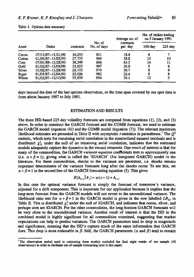
The forecasting methods presented above are evaluated using daily data for cocoa, corn, cotton, gold, silver, sugar, and wheat. The time span covered for each commodity varies slightly, depending on data availability, but usually extends from about January 1987 to November 1990. The ISD-based forecasts require data on futures prices, interest rates, and options prices. The futures data is daily closing prices, obtained from Knight-Ridder Financial Services. The interest rates we use are the Treasury-bill rates from the bill which expires closest to the time the option expires, as provided by Data Resources, Inc. The options price data for corn and wheat is daily closing prices, obtained from the Chicago Board of Trade, while the rest of the options data is daily closing prices, obtained from Data Resources, Inc. Information regarding the features of various options and futures contracts (such as the last trading day, contract months, etc.) is taken from the descriptions published by the different commodity exchanges. Table I provides a brief overview of the options data by commodity and serves to illustrate the magnitude of the data sets and the breadth of contracts traded per day. Most of Table I is self- explanatory, except perhaps the final two columns. These give the number of unique options (i.e. the number of different exercise prices) which were available with expirations close to 100 days and 225 days, respectively, on 5 January 1990.

forecasts require spot price data, which was obtained from Data Resources, Inc. In order to evaluate the forecasts, a measure of the ‘true’ 225-day volatility is needed. One measure used in the literature and the one which we use here, is the realized standard deviation of returns over the forecast horizon. This is computed by calculating the square root of the average daily squared spot return over the forecast horizon. This is called ACTUAL to represent the actual volatility of returns over the period of interest. Clearly, comparing the various long-run forecasts to ACTUAL requires spot data which extends 225

The GARCH,,T and

K . F. Kroner, K. P. Kneafsey and S . Claessens Forecasting Volatilih, 85

Table I. Options data summary

Asset

Cocoa Cotton Corn Gold Silver

Wheat sugar

Dates contracts No. of

No. of days

Average no. of contracts Per day

No. of strikes trading on 5 January 1991

100-day 225-day

07/13/87- 11 121 190 01 /05/87- 11 /02/90 07/01/88-11/28/90 01 102187-12/06/90 01 /02/87- 11 /28/90 01 /05/87-12/04/90 01 /02/87-12/10/90

16,033 27,735 38,349 25,625 26,122 22,026 35,859

85 1 964 606 987 979 982 994

18.8 28.8 63.3 26.0 26.7 22.4 36.1

8 7 15 10 14 11 9 6 8 9 9 8 12 3

days beyond the date of the last options observation, so the time span covered by our spot data is from about January 1987 to July 1991.

ESTIMATION AND RESULTS

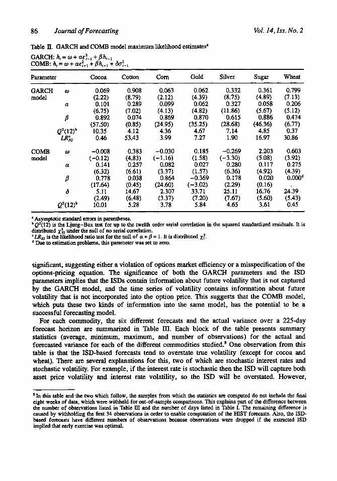
The three ISD-based 225-day volatility forecasts are computed from equations (l), (2), and (3) above. In order to construct the GARCH forecast and the COMB forecast, we need to estimate the GARCH model (equation (4)) and the COMB model (equation (7)). The relevant maximum likelihood estimates are presented in Table 11 with asymptotic t-statistics in parentheses.’ The Q2

statistic, which tests for remaining serial correlation in the standardized squared residuals and is distributed x:2 under the null of no remaining serial correlation, indicates that the estimated models adequately capture the dynamics in the second moments. One result of interest is that for many of the commodities, the GARCH variance equation coefficients sum to approximately one (i.e. a + b = l), giving what is called the ‘IGARCH’ (for Integrated GARCH) model in the literature. For these commodities, shocks to the variance are persistent, i.e. shocks remain important determinants of the variance forecasts long after the shocks occur. To see this, set a + /3 = 1 in the second line of the GARCH forecasting equation (5). This gives

m+, 19,) = O ( S - 1) + h + l

In this case the optimal variance forecast is simply the forecast of tomorrow’s variance, adjusted for a drift component. This is important for our application because it implies that the long-term forecast from the GARCH models will not revert to the unconditional variance. The likelihood ratio test for a + p = 1 in the GARCH model is given in the row labelled L& in Table II. This is distributed x: under the null of IGARCH, and indicates that cocoa, silver, and perhaps corn are IGARCH. For the other commodities, the long-horizon GARCH forecasts will be very close to the unconditional variance. Another result of interest is that the ISD in the combined model is highly significant for all commodities examined, suggesting that market expectations can help to predict variances. The GARCH parameters tend to drop in magnitude and significance, meaning that the ISD’s capture much of the same information that GARCH does. This drop is most noticeable in B. Still, the GARCH parameters (a and 8) tend to remain

‘The observation period used in estimating these models excluded the final eight weeks of our sample (40 observations) in order to facilitate out-of-sample forecasting later in this paper.


Table II. GARCH and COMB model maximum likelihood estimates' GARCH: h, = w + a&:-1 + ,f?h,-, COMB: h, = o + a&:-, + #?h,-, + &:-, Parameter Cocoa Cotton Corn Gold Silver Sugar Wheat ~ ~~

GARCH w model

a

COMB w model

a

B B

Q2(Wb

0.069 (2.22) 0.101

(6.75) 0.892

(57 SO) 10.35 0.46

-0.008 (-0.12)

0.141 (6.32) 0.778

(17.64) 5.11

(2.49) 10.01

0.908 (8.79) 0.289

(7.02) 0.074

(0.85) 4.12

53.43

0.383 (4.83) 0.257

(6.61) 0.038

(0.45) 14.67 (6.48) 5.28

0.063 (2.12) 0.099 (4.13) 0.869

(24.95) 4.36 3.99

-0.030 (- 1.16)

0.082 (3.37) 0.864

(24.60) 2.307

(3.37) 3.78

0.062 (4.39) 0.062

(4.82) 0.870

(35.25) 4.67 7.27

0.185 (1.58) 0.027

(1.57) -0.369

(-3.02) 33.71 (7.20) 5.84

0.332 (8.75) 0.327

( 1 1 36) 0.615

(28.68) 7.14 1.90

-0.269 (-3.30)

0.280 (6.36) 0.178

(2.29) 25.11' (7.67) 4.65

0.361 (4.89) 0.058 (5.67) 0.886

(46.36) 4.85

16.97

2.203 (5.08) 0.117

(4.92) 0.020

(0.16) 16.76 (5.60) 3.61

0.799 (7.13) 0.206

(5.12) 0.474

(6.77) 0.37

30.86

0.603 (3.92) 0.275

(4.39) 0.000*

24.39 (5.43) 0.45

a Asymptotic standard mom in parentheses.

distributed x:2 under the null of no serial correlation. 'LRIG is the likelihood ratio test for the null of a + /3 = 1. It is distributed 1:. * Due to estimation problems, this parameter was set to zero.

Q2(12) is the Ljung-Box test for up to the twelth order serial correlation in the squared standardized residuals. It is

significant, suggesting either a violation of options market efficiency or a misspecification of the options-pricing equation. The significance of both the GARCH parameters and the ISD parameters implies that the ISDs contain information about future volatility that is not captured by the GARCH model, and the time series of volatility contains information about future volatility that is not incorporated into the option price. This suggests that the COMB model, which puts these two kinds of information into the same model, has the potential to be a successful forecasting model.

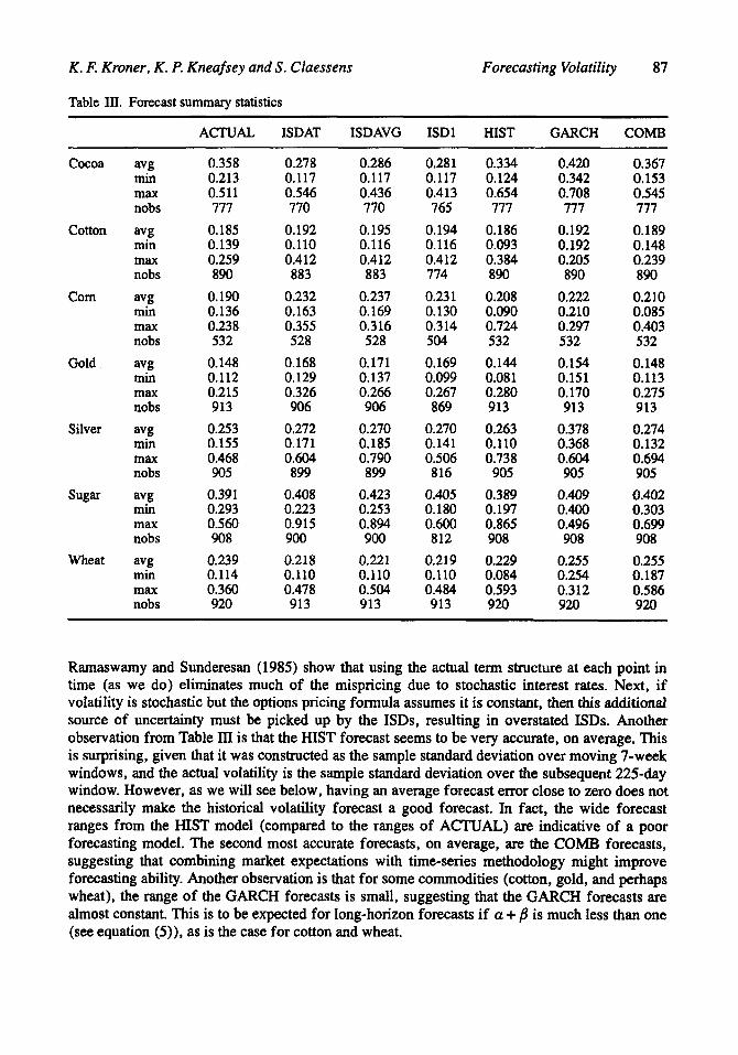
For each commodity, the six different forecasts and the actual variance over a 225-day forecast horizon are summarized in Table III. Each block of the table presents summary statistics (average, minimum, maximum, and number of observations) for the actual and forecasted variance for each of the different commodities studied.' One observation from this table is that the ISD-based forecasts tend to overstate true volatility (except for cocoa and wheat). There are several explanations for this, two of which are stochastic interest rates and stochastic volatility. For example, if the interest rate is stochastic then the ISD will capture both asset price volatility and interest rate volatility, so the ISD will be overstated. However,

In this table and the two which follow, the samples from which the statistics are computed do not include the h a l eight weeks of data, which were withheld for out-of-sample comparisons. This explains part of the difemce between the number of observations listed in Table III and the number of days listed in Table I. The remaining difference is caused by withholding the first 34 observations in order to enable computation of the HIST forecasts. Also, the ISD- based forecasts have different numbers of observations because observations were dropped if the extracted ISD implied that early exercise was optimal.

K. F. Kroner, K . P. Kneafsey and S . Claessens Forecasting Volatility 87

Table In. Forecast summary statistics

ACTUAL ISDAT ISDAVG ISDl HIST GARCH COMB

Cocoa

Cotton

Corn

Gold

Silver

sugar

Wheat

avg min max nobs avg min max nobs avg min max nobs avg min max nobs avg min max nobs

mm max nobs

mm max nobs

avg

avg

0.358 0.213 0.5 11 777

0.185 0.139 0.259 890

0.190 0.136 0.238 532

0.148 0.112 0.215 913

0.253 0.155 0.468 905

0.391 0.293 0.560 908

0.239 0.114 0.360 920

0.278 0.117 0.546 770

0.192 0.110 0.412 883

0.232 0.163 0.355 528

0.168 0.129 0.326 906

0.272 0.171 0.604 899

0.408 0.223 0.915 900 0.2 18 0.110 0.478 913

0.286 0.117 0.436 770

0.195 0.116 0.412 883

0.237 0.169 0.316 528

0.171 0.137 0.266 906

0.270 0.185 0.790 899

0.423 0.253 0.894 900

0.221 0.110 0.504 913

0.281 0.117 0.4 13 765

0.194 0.116 0.412 774 0.23 1 0.130 0.314 504 0.169 0.099 0.267 869

0.270 0.141 0.506 816

0.405 0.180 0.600 812

0.219 0.110 0.484 913

0.334 0.124 0.654 777

0.186 0.093 0.384 890 0.208 0.090 0.724 532 0.144 0.08 1 0.280 913 0.263 0.110 0.738 905

0.389 0.197 0.865 908 0.229 0.084 0.593 920

0.420 0.342 0.708 777

0.192 0.192 0.205 890

0.222 0.210 0.297 532 0.154 0.151 0.170 913

0.378 0.368 0.604 905

0.409 0.400 0.496 908

0.255 0.254 0.312 920

0.367 0.153 0.545 777 0.189 0.148 0.239 890 0.210 0.085 0.403 532 0.148 0.113 0.275 913 0.274 0.132 0.694 905 0.402 0.303 0.699 908 0.255 0.187 0.586 920

Ramaswamy and Sunderesan (1985) show that using the actual term structure at each point in time (as we do) eliminates much of the mispricing due to stochastic interest rates. Next, if volatility is stochastic but the options pricing formula assumes it is constant, then this additional source of uncertainty must be picked up by the ISDs, resulting in overstated ISDs. Another observation from Table III is that the HIST forecast seems to be very accurate, on average. This is surprising, given that it was constructed as the sample standard deviation over moving 7-week windows, and the actual volatility is the sample standard deviation over the subsequent 225-day window. However, as we will see below, having an average forecast error close to zero does not necessarily make the historical volatility forecast a good forecast. In fact, the wide forecast ranges from the HIST model (compared to the ranges of ACTUAL) are indicative of a poor forecasting model. The second most accurate forecasts, on average, are the COMB forecasts, suggesting that combining market expectations with time-series methodology might improve forecasting ability. Another observation is that for some commodities (cotton, gold, and perhaps wheat), the range of the GARCH forecasts is small, suggesting that the GARCH forecasts are almost constant. This is to be expected for long-horizon forecasts if a + /3 is much less than one (see equation (5)), as is the case for cotton and wheat.


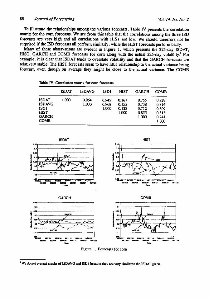
To illustrate the relationships among the various forecasts, Table IV presents the correlation matrix for the corn forecasts. We see from this table that the correlations among the three ISD forecasts are very high and all correlations with HIST are low. We should therefore not be surprised if the ISD forecasts all perform similarly, while the HIST forecasts perform badly.

Many of these observations are evident in Figure 1, which presents the 225-day ISDAT, HIST, GARCH and COMB forecasts for corn along with the actual 225-day volatility.’ For example, it is clear that ISDAT tends to overstate volatility and that the GARCH forecasts are relatively stable. The HIST forecasts seem to have little relationship to the actual variance being forecast, even though on average they might be close to the actual variance. The COMB

Table IV Correlation matrix for corn forecasts

ISDAT ISDAVG ISDl HIST GARCH COMB

ISDAT 1 .Ooo 0.964 0.945 0.167 0.755 0.829 ISDAVG 1 .Ooo 0.968 0.155 0.738 0.816 ISDl 1.Ooo 0.128 0.712 0.809 HIST 1 .om 0.855 0.313 GARCH 1.OOO 0.741 COMB 1 .Ooo

ISDAT HIST

GARCH COMB

0 I & 80120 WWl6 @W110 OOO.16 ow010 miim a m a s (0009 (00131 WOM m i m MllW - 190119 -31 *I*p7 01123

DI Dab

Figure 1. Forecasts for corn

We do not present graphs of ISDAVG and ISDl because they are very similar to the ISDAT graph.

K . F. Kroner, K . P. Kneafsey and S . Claessens Forecasting Volatilio 89

forecasts seem to track the true volatility quite well, though the swings in the COMB forecast are much larger than the swings in the realized volatility. In general, plots of the time-series forecasts are much smoother than plots of the ISD forecasts. It appears that market expectations of volatility are revised frequently, and often quite significantly.

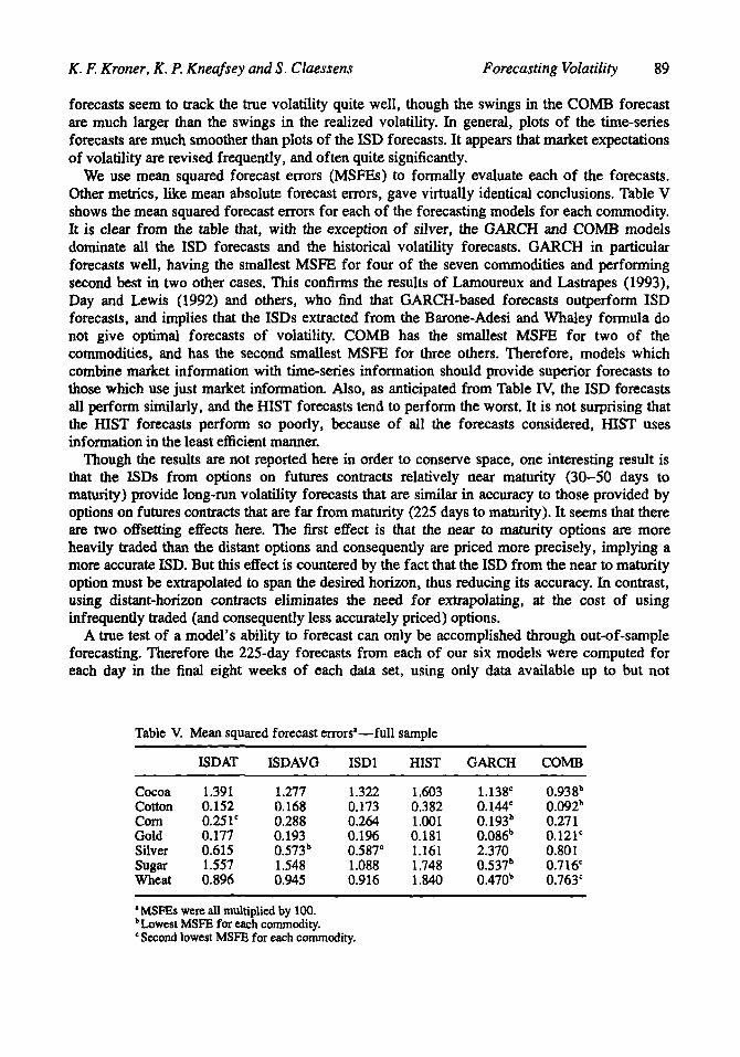
We use mean squared forecast errors (MSFEs) to formally evaluate each of the forecasts. Other metrics, like mean absolute forecast errors, gave virtually identical conclusions. Table V shows the mean squared forecast errors for each of the forecasting models for each commodity. It is clear from the table that, with the exception of silver, the GARCH and COMB models dominate all the ISD forecasts and the historical volatility forecasts. GARCH in particular forecasts well, having the smallest MSFE for four of the seven commodities and performing second best in two other cases. This confirms the results of Lamoureux and Lastrapes (1993), Day and Lewis (1992) and others, who find that GARCH-based forecasts outperform ISD forecasts, and implies that the ISDs extracted from the Barone-Adesi and Whaley formula do not give optimal forecasts of volatility. COMB has the smallest MSFE for two of the commodities, and has the second smallest MSFE for three others. Therefore, models which combine market information with time-series information should provide superior forecasts to those which use just market information. Also, as anticipated from Table IV, the ISD forecasts all perform similarly, and the HIST forecasts tend to perform the worst. It is not surprising that the HIST forecasts perform so poorly, because of all the forecasts considered, HIST uses information in the least efficient manner.

Though the results are not reported here in order to conserve space, one interesting result is that the ISDs from options on futures contracts relatively near maturity (30-50 days to maturity) provide long-run volatility forecasts that are similar in accuracy to those provided by options on futures contracts that are far from maturity (225 days to maturity). It seems that there are two offsetting effects here. The first effect is that the near to maturity options are more heavily traded than the distant options and consequently are priced more precisely, implying a more accurate ISD. But this effect is countered by the fact that the ISD from the near to maturity option must be extrapolated to span the desired horizon, thus reducing its accuracy. In contrast, using distant-horizon contracts eliminates the need for extrapolating, at the cost of using infrequently traded (and consequently less accurately priced) options.

A true test of a model's ability to forecast can only be accomplished through out-of-sample forecasting. Therefore the 225-day forecasts from each of our six models were computed for each day in the final eight weeks of each data set, using only data available up to but not

Table V. Mean squared forecast errors"-full sample

ISDAT ISDAVG ISDl HIST GARCH COMB

Cocoa 1.391 1.277 1.322 1.603 1.138' 0.938b Cotton 0.152 0.168 0.173 0.382 0.144' 0.092b Corn 0.251' 0.288 0.264 1.001 0.193b 0.271 Gold 0.177 0.193 0.196 0.181 0.086b 0.121' Silver 0.615 0.573b 0.587' 1.161 2.370 0.801 Sugar 1.557 1.548 1.088 1.748 0.537b 0.716' Wheat 0.896 0.945 0.916 1.840 0.470b 0.763'

' MSFEs were all multiplied by 100. bLowest MSFE for each commodity. 'Second lowest MSFE for each commodity.


including the final eight weeks. This gives us a time series of 40 out-of-sample forecasts from each forecasting method," for each commodity.

One additional forecast was prepared for the out-of-sample testing, which can be viewed as an alternative way of combining market-based forecasts (ISDs) and time-series based forecasts (GARCH and HIST). Granger and Ramanathan (1984) argue that if a set of forecasts exists which are based either on different information sets or on the same information set but constructed differently, then a better forecast can be obtained by combining the existing forecasts. In our situation, we have forecasts which are constructed from different information sets (e.g. the GARCH forecasts are based on historical information and the ISD forecasts, on current market expectations), as well as forecasts constructed from the same information set but constructed differently (e.g. the HIST forecasts and the GARCH forecasts are both based strictly on historical information, but the forecasts are constructed differently). Therefore, combining these forecasts has the potential to generate an improved forecast.

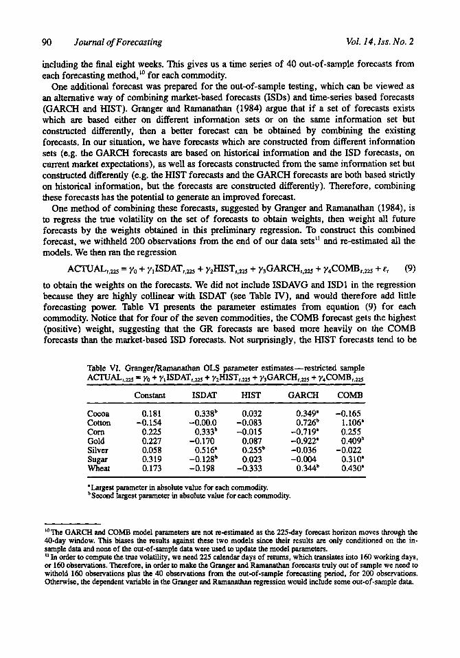
One method of combining these forecasts, suggested by Granger and Ramanathan (1984), is to regress the true volatility on the set of forecasts to obtain weights, then weight all future forecasts by the weights obtained in this preliminary regression. To construct this combined forecast, we withheld 200 observations from the end of our data sets" and re-estimated all the models. We then ran the regression

Am&,225 = YO + ~11sDATr.2~ + ~2mSTt.225 + Y~GARCH,~S + ~4COmt.225 + Er (9) to obtain the weights on the forecasts. We did not include ISDAVG and ISDl in the regression because they are highly collinear with ISDAT (see Table IV), and would therefore add little forecasting power. Table VI presents the parameter estimates from equation (9) for each commodity. Notice that for four of the seven commodities, the COMB forecast gets the highest (positive) weight, suggesting that the GR forecasts are based more heavily on the COMB forecasts than the market-based ISD forecasts. Not surprisingly, the HIST forecasts tend to be

Table VI. Granger/Ramanathan OLS parameter estimates-restricted sample AcTuAL,,m = Yo + YJSDAT,.zZs + YzHIST,,2zs + Y3GARCH,,m + Y4COMB,,m

constant ISDAT HIST GARCH COMB

Cocoa 0.181 0.338b 0.032 0.349' -0.165 Cotton -0.154 -0.00.0 -0.083 0.726b 1.106* Corn 0.225 0.333b -0.015 -0.719' 0.255 Gold 0.227 -0.170 0.087 -0.922' 0.40gb Silver 0.058 0.516' 0.255b -0.036 -0.022 sugar 0.319 -0.128b 0.023 -0.004 0.310' Wheat 0.173 -0.198 -0.333 0.3Mb 0.430'

'Largest parameter in absolute value for each commodity. Second largest parameter in absolute value for each commodity.

lo The GARCH and COMB model parameters are not re-estimated as the 225-day forecast horizon moves through the 40day window. This biases the results against these two models since their results are only conditioned on the in- sample data and none of the out-of-sample data were used to update the model parameters. I' In order to compute the true volatility, we need 225 calendar days of retums, which translates into 160 working days, or 160 observations. Therefore, in order to make the Granger and Ramanathan forecasts truly out of sample we need to withold 160 observations plus the 40 observations from the out-of-sample forecasting period, for 200 observations. Otherwise, the dependent variable in the Granger and Ramanathan regression would include some out-of-sample data.

K. I? Kroner, K. P. Kneafsey and S . Claessens Forecasting Volatility 91

unimportant, as indicated by the relatively low weights being applied to this forecast. The negative weights which sometimes appear on the GARCH forecasts can be attributed to multicollinearity with the constant. They all become positive when the constant term is omitted from the regression.12 This linear combination of forecasts is guaranteed to provide within- sample forecasts that are superior to any of the individual forecasts because it is chosen to minimize within-sample mean squared forecast error. This suggests, but does not guarantee, that it will perform better out-of-sample as well.

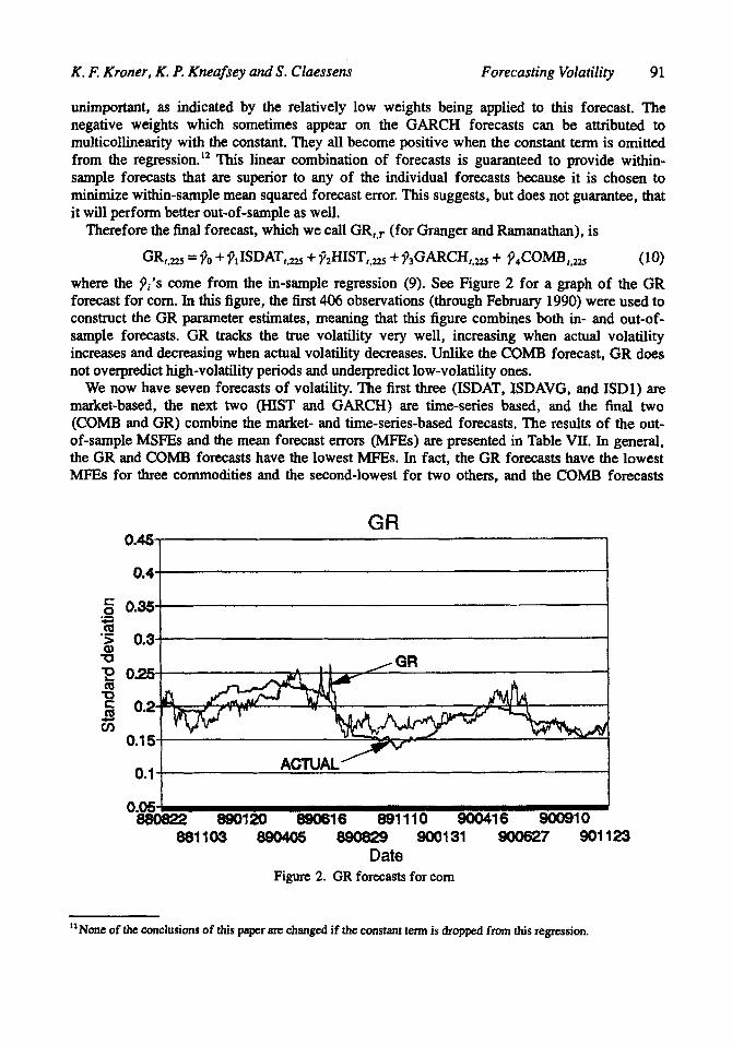
Therefore the final forecast, which we call GR,, (for Granger and Ramanathan), is

GRf,225 = 9 0 + ?11SDATf.ZZ5 + f2H1STf,225 + ?3GARCHf,225 + P4c0MBf,2U (10) where the Pi 's come from the in-sample regression (9). See Figure 2 for a graph of the GR forecast for corn. In this figure, the first 406 observations (through February 1990) were used to construct the GR parameter estimates, meaning that this figure combines both in- and out-of- sample forecasts. GR tracks the true volatility very well, increasing when actual volatility increases and decreasing when actual volatility decreases. Unlike the COMB forecast, GR does not overpredict high-volatility periods and underpredict low-volatility ones.

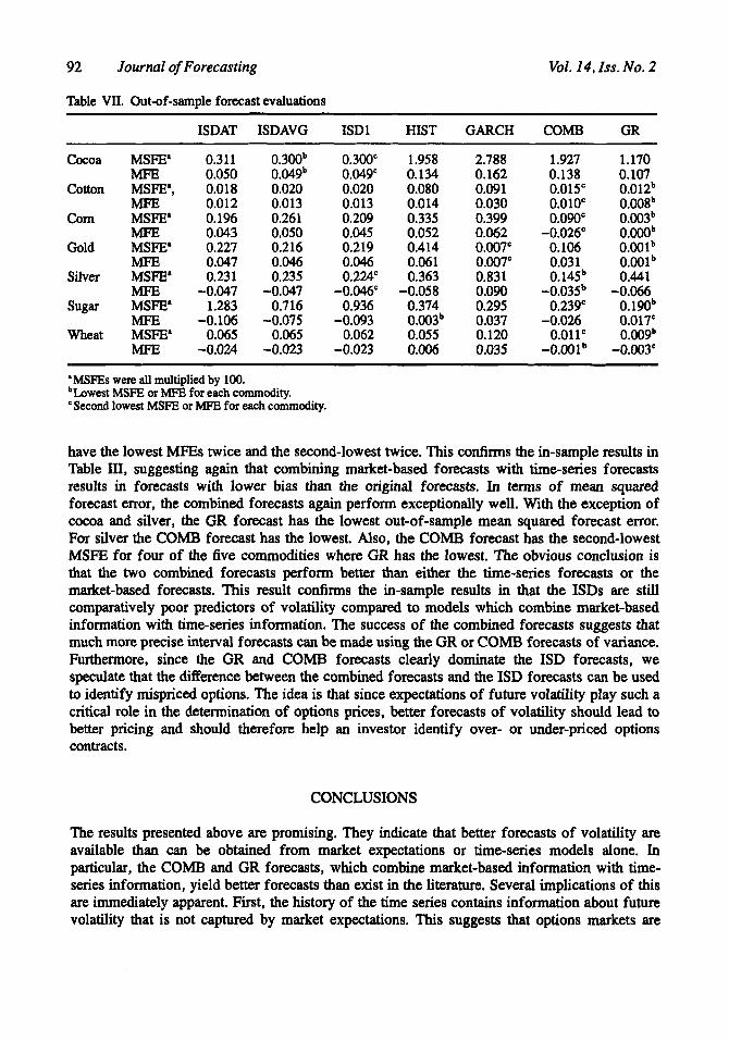
We now have seven forecasts of volatility. The first three (ISDAT, ISDAVG, and ISD1) are market-based, the next two (HIST and GARCH) are time-series based, and the final two (COMB and GR) combine the market- and time-series-based forecasts. The results of the out- of-sample MSFEs and the mean forecast errors (MFEs) are presented in Table W. In general, the GR and COMB forecasts have the lowest MFEs. In fact, the GR forecasts have the lowest MFEs for three commodities and the second-lowest for two others, and the COMB forecasts

GR 0.45 I 1

ACTUAL 0.1

0.05 880822 890120 890616 891110 900416 900910

881103 890405 890829 900131 900627 901123 Date

Figure 2. GR forecasts for corn

''None of the conclusions of this paper changed if the constant term is dropped from this regression.


Table VII. Out-of-sample forecast evaluations

Cocoa

Cotton

COm

Gold

Silver

sugar

Wheat

ISDAT

MSFE' 0.3 11 MFE 0.050 MSFE', 0.018 MFE 0.012 MSFE' 0.196 MFE 0.043 MSFE' 0.227 MFE 0.047 MSFE' 0.23 1 m -0.047 MSFE' 1.283 MFE -0.106 MSFE' 0.065 MFE -0.024

ISDAVG

0.3Mb 0.04gb 0.020 0.013 0.261 0.050 0.216 0.046 0.235

-0.047 0.716

-0.075 0.065

-0.023

ISD 1

0.300' 0.049' 0.020 0.013 0.209 0.045 0.219 0.046 0.224'

-0.046' 0.936

-0.093 0.062

-0.023

HIST GARCH COMB GR

1.958 0.134 0.080 0.014 0.335 0.052 0.414 0.061 0.363

0.374 0.003b 0.055 0.006

-0.058

2.788 0.162 0.091 0.030 0.399 0.062 0.007' 0.007' 0.831 0.090 0.295 0.037 0.120 0.035

1.927 0.138 0.015' 0.010' 0.090'

-0.026' 0.106 0.031 0.145b

-0.035b 0.239'

-0.026 0.011'

-O.OOlb

1.170 0.107 0.012b 0.008b 0.003b 0.0OOb O.OOlb O.OOlb 0.441

-0.066 0.19Ob 0.017' O.OOgb

-0.003'

'MSFEs w m all multiplied by 100. bLowest MSFE or MFE for each commodity. Second lowest MSFE or MFE for each commodity.

have the lowest MFEs twice and the second-lowest twice. This confirms the in-sample results in Table ID, suggesting again that combining market-based forecasts with time-series forecasts results in forecasts with lower bias than the original forecasts. In terms of mean squared forecast error, the combined forecasts again perform exceptionally well. With the exception of cocoa and silver, the GR forecast has the lowest out-of-sample mean squared forecast error. For silver the COMB forecast has the lowest. Also, the COMB forecast has the second-lowest MSFE for four of the five commodities where GR has the lowest. The obvious conclusion is that the two combined forecasts perform better than either the time-series forecasts or the market-based forecasts. This result confirms the in-sample results in that the ISDs are still comparatively poor predictors of volatility compared to models which combine rnarket-based information with time-series information. The success of the combined forecasts suggests that much more precise interval forecasts can be made using the GR or COMB forecasts of variance. Furthermore, since the GR and COMB forecasts clearly dominate the ISD forecasts, we speculate that the difference between the combined forecasts and the ISD forecasts can be used to identify mispriced options. The idea is that since expectations of future volatility play such a critical role in the determination of options prices, better forecasts of volatility should lead to better pricing and should therefore help an investor identify over- or under-priced options contracts.

CONCLUSIONS

The results presented above are promising. They indicate that better forecasts of volatility are available than can be obtained from market expectations or time-series models alone. In particular, the COMB and GR forecasts, which combine market-based information with time- series information, yield better forecasts than exist in the literature. Several implications of this are immediately apparent. First, the history of the time series contains information about future volatility that is not captured by market expectations. This suggests that options markets are

K. F. Kroner, K. P. Kneafsey and S. Claessens Forecasting Volatility 93

inefficient and/or the option-pricing formula we used is incorrect. This implies it is possible that our volatility forecast can be used to identify mispriced options, and a profitable trading rule could be established based on the difference between the ISD and the COMB or GR volatility forecast. Second, our forecasting method can be used to obtain interval forecasts of commodity prices, which should be beneficial to market participants who are concerned about the precision of a point forecast, or to policy makers whose policies will depend on volatility forecasts. One final note is that the accurate matching of the forecast horizon and the time to maturity of the futures contract is relatively unimportant. Our results indicate that near to maturity options tend to forecast long-run volatility about as well as options that are far from maturity.

APPENDIX

Suppose that the underlying futures price follows the stochastic dserential equation

dF/F= f d t + a d z (Al) where F is the commodity futures price, f is the instantaneous expected relative price change of the commodity, (7 is the instantaneous standard deviation, t is time, and z is a Wiener process. "hen if the interest rate r is constant and no arbitrage opportunities exist, Black (1976) shows that the price of a commodity futures option, C, must follow the partial differential equation

(W 1 2 2 2~ F C F F - r C + C , = O

where subscripts represent partial derivatives of the variable with respect to the subscript. For a European option with no early exercise privilege, the boundary condition requires that the maturity value of the option be equal to max(0, F T - X}, where FT is the future price at maturity and X is the exercise price. This boundary condition is applied to equation (A2) to get Black's European commodity futures option pricing formula

(A31 M , , T , r, X, 0) = e-fl[Ffl(dl 1 - X W 2 ) 1 where T is time to maturity, N(.) is the cumulative normal distribution, and

dl = [In(F,/X) + f Tu2]ul? d2 = dl - d\lT

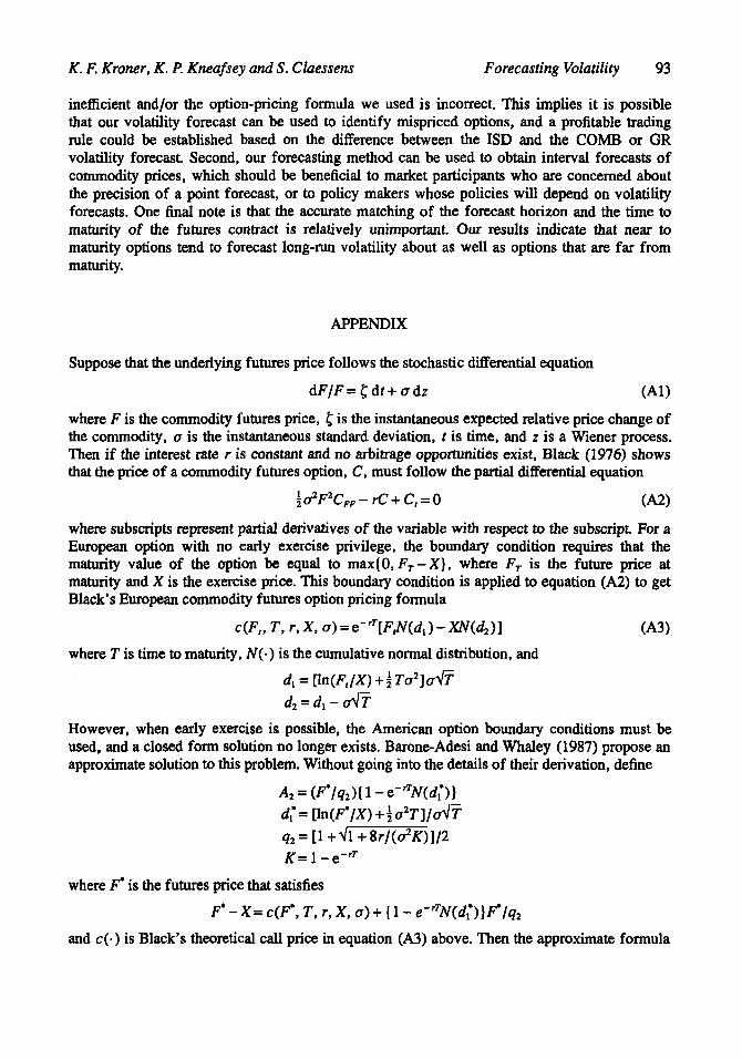
However, when early exercise is possible, the American option boundary conditions must be used, and a closed form solution no longer exists. Barone-Adesi and Whaley (1987) propose an approximate solution to this problem. Without going into the details of their derivation, define

Az = (F'/qz)( 1 - eerTN(d;)} d; = F ( F * / X ) + a2T]/6\(? q2= [l +dl +8r/(a2K)]/2 K = 1 -e-fl

where F' is the futures price that satisfies

F'- X = c(F', T, r, X, a) + { 1 - e-'TN(d;)}F./42

and c(.) is Black's theoretical call price in equation (A3) above. Then the approximate formula


for the price of an American commodity futures call option at time t , C(F,, T, r, X, a), is

ACKNOWLEDGEMENTS

We would like thank seminar participants at the World Bank and the University of Arizona and an anonymous referee for their useful suggestions. All errors are ours alone. The opinions expressed herein are not those of the World Bank.

REFERENCES

Akigray, V., ‘Conditional heteroskedasticity in time series models of stock returns: evidence and forecasts’, Journal of Business, 62 (1989), 55-99

Baillie, R. T., Bollerslev, T. and Mikkelsen, H. O., ‘Fractionally integrated generalized autoregressive conditional heteroskedaticity’, unpublished manuscript, J. L. Kellogg Graduate School of Management, Northwestern University, 1993.

Barone-Adesi, G. and Whaley, R. E., ‘Efficient analytic approximation of American option values’, Journal of Finance, 42 (1987), 301-320.

Bartunek, K. and Mustafa, C., ‘Implied volatility vs. GARCH: a comparison of forecasts’, Managerial Finance, forthcoming (1994).

Beckers, S., ‘Variances of security price returns based on high, low and closing prices’, Journal of Business, 56 (1993), 97-112.

Black, F., ‘The pricing of commodity contracts’, Journal of Financial Economics, 3 (1976), 167-79. Bollerslev, T., ‘Generalized autoregressive conditional heteroskedasticity’, Journal of Econometrics, 31

Bollerslev, T., Chou, R. Y. and Kroner, K. F., ‘ARCH modeling in finance: a review of the theory and empirical evidence’, Journal of Econometrics, 52 (1992), 5-60.

Bollerslev, T. and Mikkelsen, H. O., ‘Modelling and pricing long-memory in stock market volatility’, unpublished manuscript, J. L. Kellogg Graduate School of Management, Northwestern University, 1993.

Cao, C. Q. and Tsay, R. S., ‘Nonlinear time series analysis of stock volatilities’, Journal of Applied Econometrics, 7 (1992). 165-85.

Day, T. E. and Lewis, C. M., ‘Stock market volatility and the information content of stock index options’, Journal of Econometrics, 52 (1992), 267-87.

Engle, R. F., ‘Autoregressive conditional heteroskedasticity with estimates of the variance of U.K inflation’, Econometrica, 50 (1982), 987-1007.

Engle, R. F. and Bollerslev, T., ‘Modeling the persistence of conditional variances’, Econometric Reviews,

Granger, C. W. and Ramanathan, R., ‘Improved methods of combining forecasts’, Journal of

Hull, J. and White. A., ‘The pricing of options with stochastic volatility’, Journal of Finance, 42 (1987),

Lamoureux, C. G. and Lastrapes, W. D., ‘Forecasting stock return variance: toward an understanding of

Latane, H. A. and Rendleman, R. J., ‘Standard deviations of stock price ratios implied in option prices’,

Poterba, J. and Summers, L., ‘The persistence of volatility and stock market fluctuations’, American

(1986), 307-327.

5 (1986), 1-50.

Forecusting, 3 (1984), 197-204.

281-300.

stochastic implied volatilities’, Review of Financial Studies, 6(2) (1993), 293-326.

Journal of Finance, 31 (1976), 369-81.

Economic Review 76 (1986). 1142-51.

K . F. Kroner, K . P. Kneafsey and S. Claessens Forecasting Volatility 95

Ramaswamy, K. and Sundaresan, S. M., ‘The valuation of American options on futures contracts’,

Stein, J., ‘Overreactions in the options market’, Journal of Finance, 44(4) (1989), 1011-23. Taylor, S. J., ‘Forecasting the volatility of c m c y exchange rates’, International JOUMU~ of Forecasting.

Wei, S . J. and Frankel, J. A., ‘Are option-implied forecasts of exchange rate volatility excessively

Journal of Finance, 40 (1985), 1318-40.

3 (1987), 159-70.

variable?’ unpublished manuscript, NBER Working Paper No. 3910, 1991.

Authors’ biographies: Kenneth F. Kroner received his Ph.D. in economics from UC San Diego in 1988. He is currently an Associate Professor of Economics and Finance at the University of Arizona and a Principal at Wells Fargo Nikko Investment Advisors. His areas of research include volatility modeling and forecasting global asset markets. Kevin P. Kneafsey received his Ph.D. in finance from the University of Arizona in 1995. He is currently employed by the Defined Contributions group at Wells Fargo Nikko Investment Advisors, where his main responsibility is product development. His areas of interest include asset pricing and risk modeling. Stun Claessens is a senior financial economist in the private Sector and Finance Division of the Technical Department for the East Europe, Central Asia and Middle East regions at the World Bank. He holds a Ph.D. in business economics from the Wharton School of the University of Pennsylvania. Previously, he taught at NYU. His research inkrests are how countries can manage their external risks; alternative forms of financing available for development; and enterprise restructuring in transition economies.

Authors’ addresses: Kenneth F. Kroner, Advanced Strategies and Research Group, Wells Fargo Nikko Investment Advisors, 45 Fremont Street, San Francisco, CA 94105, USA. Kevin P. Kneafsey, Wells Fargo Nikko Investment Advisors, 2180 West S.R. 434, Suite 2160, Longwood, FL 32779, USA. Stijn Claessens, Private Sector and Finance Division, Technical Department East Europe, Central Asia and Middle East, World Bank, 1818 H Street, NW, Washington, DC 20433, USA.

forecasting volatility in commodity markets

Documents