forecasting volatility by means of threshold models

Copyright © 2007 John Wiley & Sons, Ltd.

Forecasting Volatility by Means ofThreshold Models

M. PILAR MUÑOZ,1* M. DOLORES MARQUEZ2 AND LESLY M. ACOSTA1

1 Department of Statistics and Operations Research, TechnicalUniversity of Catalonia, Spain2 Department of Business Economics, Autonomous University ofBarcelona, Spain

ABSTRACTThe aim of this paper is to compare the forecasting performance of competingthreshold models, in order to capture the asymmetric effect in the volatility. We focus on examining the relative out-of-sample forecasting ability of theSETAR-Threshold GARCH (SETAR-TGARCH) and the SETAR-ThresholdStochastic Volatility (SETAR-THSV) models compared to the GARCH modeland Stochastic Volatility (SV) model. However, the main problem in evaluat-ing the predictive ability of volatility models is that the ‘true’ underlyingvolatility process is not observable and thus a proxy must be defined for theunobservable volatility. For the class of nonlinear state space models (SETAR-THSV and SV), a modified version of the SIR algorithm has been used to esti-mate the unknown parameters. The forecasting performance of competingmodels has been compared for two return time series: IBEX 35 and S&P 500.We explore whether the increase in the complexity of the model implies thatits forecasting ability improves. Copyright © 2007 John Wiley & Sons, Ltd.

key words Forecasting; SETAR-TGARCH; SETAR-THSV; importance sampling; Monte Carlo simulation techniques

INTRODUCTION

Threshold models are a special class of nonlinear model. The fundamental idea behind these modelsis the introduction of regimes based on thresholds, thus allowing the analysis of complex stochas-tic systems from simple subsystems. In this group, the self-exciting threshold autoregressive model(SETAR) is defined on the basis of an autoregressive (AR) process in each regimen, and the vari-able which governs the switching regime is the delayed process variable. The SETAR model is ableto capture the asymmetric pattern of a time series by its local property.

Numerous researchers have been attracted by this class of model. They have been used to modeltime series data in such diverse fields as oceanography (Lewis and Ray, 1997) hydrology (Lall

Journal of ForecastingJ. Forecast. 26, 343–363 (2007)Published online in Wiley InterScience(www.interscience.wiley.com) DOI: 10.1002/for.1031

* Correspondence to: M. Pilar Muñoz, Department of Statistics and Operations Research, North Campus—C5, Jordi Girona1–3, 08034 Barcelona, Spain. E-mail: [email protected]

344 M. P. Muñoz, M. D. Marquez and L. M. Acosta

Copyright © 2007 John Wiley & Sons, Ltd. J. Forecast. 26, 343–363 (2007)DOI: 10.1002/for

et al., 1996), economics (Caner and Hansen, 2004) and medical sciences (Saei, 2004). In the finan-cial time series field, thresholds models are an interesting alternative for modeling both returns andvolatility (Tong, 1990). The existence of different regimes in financial series seems natural and allowsthat the dynamic behavior of time series depends on the regime that occurs. The definition of theregimes by the introduction of thresholds supposes a flexible structure.

Le Baron (1992) shows that the correlations of stock return are related to the level of volatilityof these returns and that the periods of low and high volatility can be interpreted as distinct regimes.Also, empirical evidence suggests that large returns tend to be followed by large returns and smallreturns by small returns. The idea of using the variable of process delayed to govern the dynamicpattern of stock volatility appears to be natural and is in good agreement with the concept of SETARmodel. Cao and Tsay (1992) showed that SETAR models provided better forecasts than the previ-ous family of conditional heteroskedastic models.

The introduction of thresholds in conditional heteroskedastic models as Generalized Autoregres-sive Conditional Heteroskedastic model (GARCH(1, 1)) and Stochastic Volatility models (SV)allows one to capture the asymmetry of volatility. Earlier models (SETAR, GARCH and SV) belongto the class of ‘first-generation models’ and the result of the introduction of thresholds is the Thresh-old GARCH (TGARCH) model (see Glosten et al., 1993; Zakoian, 1994) or Threshold StochasticVolatility (THSV) (So et al., 2002). For a review of those models see Franses and van Dijk (2000)and the references contained therein.

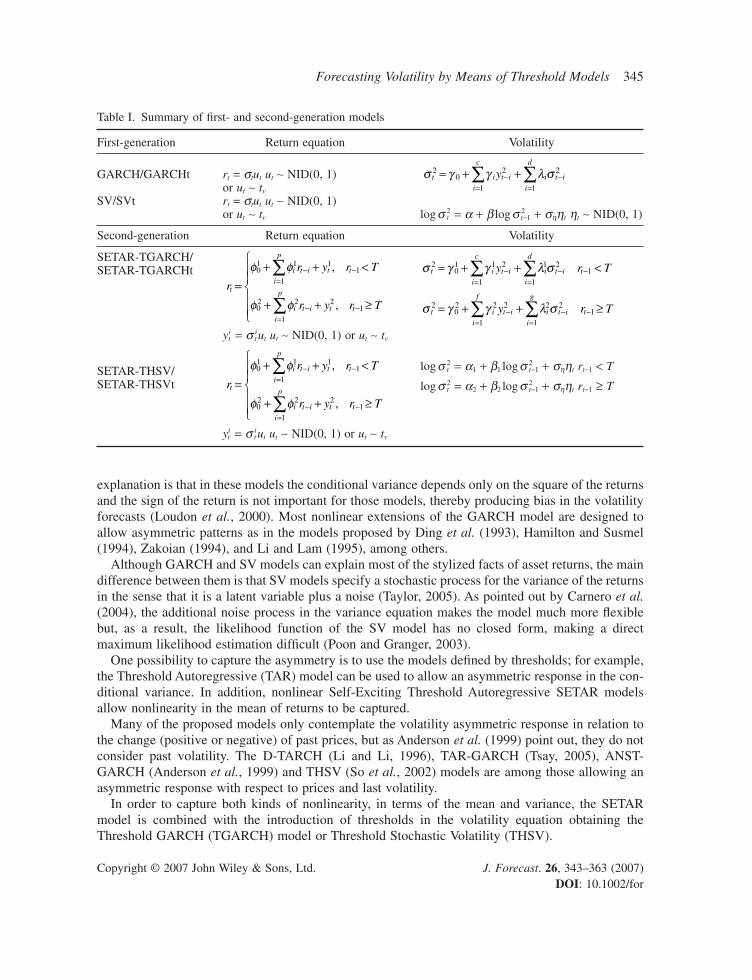
The previous models are combined to explain nonlinearity, in terms of the mean and in variance,obtaining the self-exciting threshold autoregressive threshold GARCH (SETAR-TGARCH) modeland the self-exciting threshold autoregressive threshold stochastic volatility (SETAR-THSV) model,which are known as ‘second-generation models’ (see Table I).

The aim of this paper is to compare the forecasting performance of competing models, in orderto capture the asymmetric effect in the volatility. We focus on examining the relative out-of-sampleforecasting ability of the SETAR-TGARCH model and the SETAR-THSV model compared to theGARCH model and SV model. However, the main problem of evaluating the predictive ability ofvolatility models is that the ‘true’ underlying volatility process is not observable and thus a proxymust be defined for the unobservable volatility. To attain our proposal, the proxy volatility measureand the loss function must be adequately chosen to ensure a correct ranking of models.

This paper is organized as follows. The next section provides an overview of the SETAR-TGARCH and SETAR-THSV models and several estimation algorithms are presented, most of thembased in nonlinear particle filtering. The third section presents the Monte Carlo study in order toverify the quality of the estimation procedures; in the fourth section we focus on comparison of themodels, and then we discuss the choice of volatility proxy and loss function. The fourth sectionfocuses on empirical findings, and in the final section we present the concluding remarks.

MODELS

The Generalized Autoregressive Conditional Heteroskedastic model (GARCH(1, 1)) and StochasticVolatility model (SV) are the nonlinear time series models most commonly used in the finance lit-erature to study the behavior of the returns and its volatility. An important characteristic, known asthe leverage effect, is related to the asymmetric behavior of the market, in the sense that it is morevolatile after a continuous decrease in prices than after a rise (both of the same magnitude). However,GARCH models cannot capture the asymmetry of volatility (Anderson et al., 1999); one possible

Forecasting Volatility by Means of Threshold Models 345


explanation is that in these models the conditional variance depends only on the square of the returnsand the sign of the return is not important for those models, thereby producing bias in the volatilityforecasts (Loudon et al., 2000). Most nonlinear extensions of the GARCH model are designed toallow asymmetric patterns as in the models proposed by Ding et al. (1993), Hamilton and Susmel(1994), Zakoian (1994), and Li and Lam (1995), among others.

Although GARCH and SV models can explain most of the stylized facts of asset returns, the maindifference between them is that SV models specify a stochastic process for the variance of the returnsin the sense that it is a latent variable plus a noise (Taylor, 2005). As pointed out by Carnero et al.(2004), the additional noise process in the variance equation makes the model much more flexiblebut, as a result, the likelihood function of the SV model has no closed form, making a directmaximum likelihood estimation difficult (Poon and Granger, 2003).

One possibility to capture the asymmetry is to use the models defined by thresholds; for example,the Threshold Autoregressive (TAR) model can be used to allow an asymmetric response in the con-ditional variance. In addition, nonlinear Self-Exciting Threshold Autoregressive SETAR modelsallow nonlinearity in the mean of returns to be captured.

Many of the proposed models only contemplate the volatility asymmetric response in relation tothe change (positive or negative) of past prices, but as Anderson et al. (1999) point out, they do notconsider past volatility. The D-TARCH (Li and Li, 1996), TAR-GARCH (Tsay, 2005), ANST-GARCH (Anderson et al., 1999) and THSV (So et al., 2002) models are among those allowing anasymmetric response with respect to prices and last volatility.

In order to capture both kinds of nonlinearity, in terms of the mean and variance, the SETARmodel is combined with the introduction of thresholds in the volatility equation obtaining the Threshold GARCH (TGARCH) model or Threshold Stochastic Volatility (THSV).

Table I. Summary of first- and second-generation models

First-generation Return equation Volatility

GARCH/GARCHt rt = stut ut ∼ NID(0, 1)or ut ∼ tv

SV/SVt rt = stut ut ∼ NID(0, 1)or ut ∼ tv logs 2

t = a + b logs 2t−1 + shht ht ∼ NID(0, 1)

Second-generation Return equation Volatility

SETAR-TGARCH/SETAR-TGARCHt

yit = s i

tut ut ∼ NID(0, 1) or ut ∼ tv

SETAR-THSV/SETAR-THSVt

yit = s i

tut ut ∼ NID(0, 1) or ut ∼ tv

r

r y r T

r y r T

t

i t i t ti

p

i t i t ti

p=

+ + <

+ + ≥

− −=

− −=

∑

∑

f f

f f

01 1 1

11

02 2 2

11

,

,

r

r y r T

r y r T

t

i t i t ti

p

i t i t ti

p=

+ + <

+ + ≥

− −=

− −=

∑

∑

f f

f f

01 1 1

11

02 2 2

11

,

,

s g g l st i t ii

c

i t ii

d

y20

2

1

2

1

= + +−=

−=

∑ ∑

logs 2t = a1 + b1 logs 2

t−1 + shht rt−1 < T

logs 2t = a2 + b2 logs 2

t−1 + shht rt−1 ≥ T

s g g l st i t ii

f

i t ii

g

ty r T202 2 2

1

2 2

11= + + ≥−

=−

=−∑ ∑

s g g l st i t ii

c

i t ii

d

ty r T201 1 2

1

1 2

11= + + <−

=−

=−∑ ∑



SETAR modelThe family of TAR models uses piecewise linear models to obtain a better approximation of the conditional mean equation. It is, however, not a linear model in time space but a linear model in threshold space. The switching regime is governed by a threshold parameter. This makes it possible to reproduce and describe the system state such that it does not depend on the initial conditions.

The most popular TAR model is the Self-Exciting TAR (SETAR) model. In general, a SETARmodel (�; p1, . . . , p�) has � regimes with � − 1 thresholds, where d is the delay parameter of thethreshold variable and p1, . . . , p� are the orders of each autoregressive process. The switching mech-anism is controlled by the threshold variable rt−d, not by the time index t.

For example, a time series rt follows a SETAR(2; p1, p2) process if it satisfies the following model:

(1a)

(1b)

where {ut} can follow a sequence of i.i.d. Gaussian random variables with mean 0 and variance 1or a standardized Student’s-t distribution.

In this model we consider only two regimes and suppose that the delay in the threshold variabled is equal to 1; this is in agreement with the behavior of returns in financial markets. It is necessaryto estimate the values of the coefficients f j

i , the orders p1 and p2 and the threshold value T.

Estimation of SETAR(2; p1, p2)The usual approach to the estimation of SETAR models is based on Tong’s methodology and on thealgorithm proposed by Tsay in order to test a threshold nonlinearity and to estimate the coefficientsof the autoregressive processes (Tsay, 1989).

In this paper we use the TAR-F test of Tsay (1989) to detect the threshold nonlinearity and to esti-mate the delay parameter d. Then, we use the AIETC algorithm proposed by Márquez (2002) (seeAppendix 1). The AIETC algorithm is based on Tsay’s algorithm (Tsay, 1989), but introduces someimprovements in the identification and estimation processes. Particularly, to estimate the coefficients,Marquez’s algorithm allows the automatic selection of regressors as well as the automatic estimation of both the autoregressive process orders, and the threshold in SETAR models with tworegimes.

The AIETC algorithm is based in an arranged autoregression where the specified model is esti-mated by a recursive conditional least-square procedure. The minimization of AIC (Akaike’s infor-mation criteria) refines the autoregressive orders and estimates the threshold value. The specific codeis developed in Fortran 77.

SETAR model for returns with the TGARCH(1, 1) model for volatilityThis model combines a SETAR model for the mean equation with a TGARCH model for volatilitywith the goal of capturing the asymmetries in the mean and allowing an asymmetric response in theconditional variance.

A time series rt follows a SETAR(2; p1, p2)–TGARCH(1, 1) process if it satisfies the followingmodel:

y ut t t= s

rr r y r T

r r y r Tt

t p t p t t

t p t p t t

=+ + + + <

+ + + + ≥

− − −

− − −

f f f

f f f01

11

11

1

02

12

12

1

1 1

2 2

. . . ,

. . . ,



(2a)

(2b)

(2c)

(2d)

(2e)

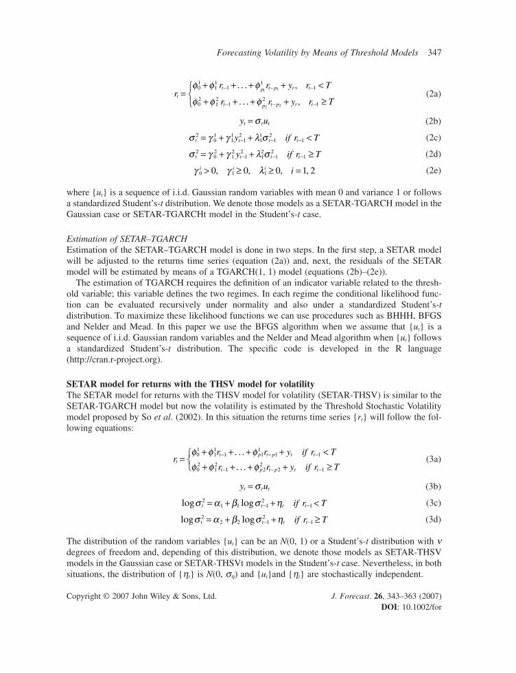
where {ut} is a sequence of i.i.d. Gaussian random variables with mean 0 and variance 1 or followsa standardized Student’s-t distribution. We denote those models as a SETAR-TGARCH model in theGaussian case or SETAR-TGARCHt model in the Student’s-t case.

Estimation of SETAR–TGARCHEstimation of the SETAR–TGARCH model is done in two steps. In the first step, a SETAR modelwill be adjusted to the returns time series (equation (2a)) and, next, the residuals of the SETARmodel will be estimated by means of a TGARCH(1, 1) model (equations (2b)–(2e)).

The estimation of TGARCH requires the definition of an indicator variable related to the thresh-old variable; this variable defines the two regimes. In each regime the conditional likelihood func-tion can be evaluated recursively under normality and also under a standardized Student’s-tdistribution. To maximize these likelihood functions we can use procedures such as BHHH, BFGSand Nelder and Mead. In this paper we use the BFGS algorithm when we assume that {ut} is asequence of i.i.d. Gaussian random variables and the Nelder and Mead algorithm when {ut} followsa standardized Student’s-t distribution. The specific code is developed in the R language(http://cran.r-project.org).

SETAR model for returns with the THSV model for volatilityThe SETAR model for returns with the THSV model for volatility (SETAR-THSV) is similar to theSETAR-TGARCH model but now the volatility is estimated by the Threshold Stochastic Volatilitymodel proposed by So et al. (2002). In this situation the returns time series {rt} will follow the fol-lowing equations:

(3a)

(3b)

(3c)

(3d)

The distribution of the random variables {ut} can be an N(0, 1) or a Student’s-t distribution with ndegrees of freedom and, depending of this distribution, we denote those models as SETAR-THSVmodels in the Gaussian case or SETAR-THSVt models in the Student’s-t case. Nevertheless, in bothsituations, the distribution of {ht} is N(0, sh) and {ut}and {ht} are stochastically independent.

log logs a b s ht t t tif r T22 2 1

21= + + ≥− −

log logs a b s ht t t tif r T21 1 1

21= + + <− −

y ut t t= s

rr r y if r T

r r y if r Tt

t p t p t t

t p t p t t

=+ + + + <+ + + + ≥

− − −

− − −

f f ff f f

01

11

1 11

1 1

02

12

1 22

2 1

. . .

. . .

g g l0 1 10 0 0 1 2i i i i> ≥ ≥ =, , , ,

s g g l st t t ty if r T202

12

12

12

12

1= + + ≥− − −

s g g l st t t ty if r T201

11

12

11

12

1= + + <− − −

y ut t t= s

rr r y r T

r r y r Tt

t p t p t t

t p t p t t

=+ + + + <

+ + + + ≥

− − −

− − −

f f f

f f f01

11

11

1

02

12

12

1

1 1

2 2

. . . ,

. . . ,



State space representation and recursive Bayesian estimation of THSV/THSVt modelsAs in the previous case, the estimation is done in two steps. In the first step, a SETAR model willbe adjusted to the returns time series (equation (3a)) and afterwards the residuals of the SETARmodel will be estimated by means of a THSV model (equations (3b)–(3d)).

The main feature of equations (3b)–(3d) is that they describe a discrete time, nonlinear dynamicsystem, which evolves as a first-order Markov process. In this case nonlinearity appears in the obser-vation equation (3b) and also in the state equations (3c) and (3d). The state is xt = log s 2

t and non-linearities in the state equations are introduced by the fact that the autoregressive process in (3c)–(3d)is determined by the sign of the previous return; in other words, a threshold nonlinear model is con-sidered for the variance of the returns. In this case, the parameters a and b switch between the tworegimes.

To estimate the unknown parameters it is necessary to resort to the Bayesian estimation because the likelihood function cannot be expressed in closed form. The usual approach is to intro-duce the unknown parameters q = (a1, a2, b1, b2, sh) in the Gaussian case or q = (a1, a2, b1, b2, n)in the Student’s-t case as part of the state vector (xt, q)′ in order to obtain the a posteriori PDF p(xt, q|Dt) when observation yt arrives at time t. Dt means the set of all the observations until timet, where Dt = {y1, . . . , yt} and n is the degrees of freedom of the Student’s-t distribution to be estimated.

So et al. (2002) proposed to estimate them using Gibbs sampling. Liu and Chen (1998) pointedout that Gibbs sampling is less attractive than importance sampling when ‘one’s interest is in realtime prediction and updating in a dynamic system’. In addition, Gibbs sampling may be ineffective‘when the states of the resulting samples are very sticky, rendering the sampler very difficult to move’in the state space.

Our approach is to estimate the a posteriori PDF using our modified version of the SamplingImportance Resampling (SIR) filter. The standard SIR filter has the problem that the particles asso-ciated with the parameters do not regenerate, meaning that there is an impoverishment problem afew iterations later. Our proposal (Muñoz et al., 2004) consists in modifying the standard SIR, addingthe jitter suggested by Liu and West (2001), to ensure that the particles cover the a posteriori distribution. The THSV_SIRJ algorithm proposed is described in Appendix 2.

MONTE CARLO STUDY

The following Monte Carlo study has been carried out in order to verify the quality of the estima-tion of the different models displayed in the previous section and summarized in Table I. Also, weconsider the classic GARCH(1, 1) model, with Student’s-t noise, and the SV models with Gaussianand Student’s-t noise. We simulated 100 series for each of the models. Although the sample size isN = 2000 observations, in each model we show the results with a sample size of length equal to thepublished results. The parameters are selected following the results published in previous papers (seeTable II), thus facilitating direct comparison in terms of the estimation parameters as well as esti-mation volatilities. The results for the models SV, SVt, SETAR-THSV and SETAR-THSVt areobtained using M = 10,000 particles in the THSV_SIRJ algorithm.

Parameter estimationWe divide this section into five subsections, according to the models shown in Table I. We avoidedshowing results from the Gaussian GARCH(1, 1) model since it is a very well-known model in the



financial literature and at this moment the estimation algorithms implemented in the statistics pack-ages are very well tested.

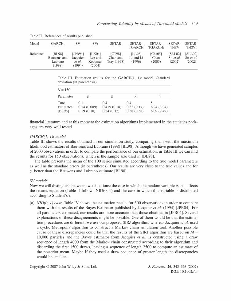
GARCH(1, 1)t modelTable III shows the results obtained in our simulation study, comparing them with the maximumlikelihood estimators of Bauwens and Lubrano (1998) [BL98]. Although we have generated samplesof 2000 observations in order to compare the performance of our estimation, in Table III we can findthe results for 150 observations, which is the sample size used in [BL98].

The table presents the mean of the 100 series simulated according to the true model parametersas well as the standard errors (in parentheses). Our results are very close to the true values and forg1 better than the Bauwens and Lubrano estimate [BL98].

SV modelsNow we will distinguish between two situations: the case in which the random variable ut that affectsthe returns equation (Table I) follows NID(0, 1) and the case in which this variable is distributedaccording to Student’s-t:

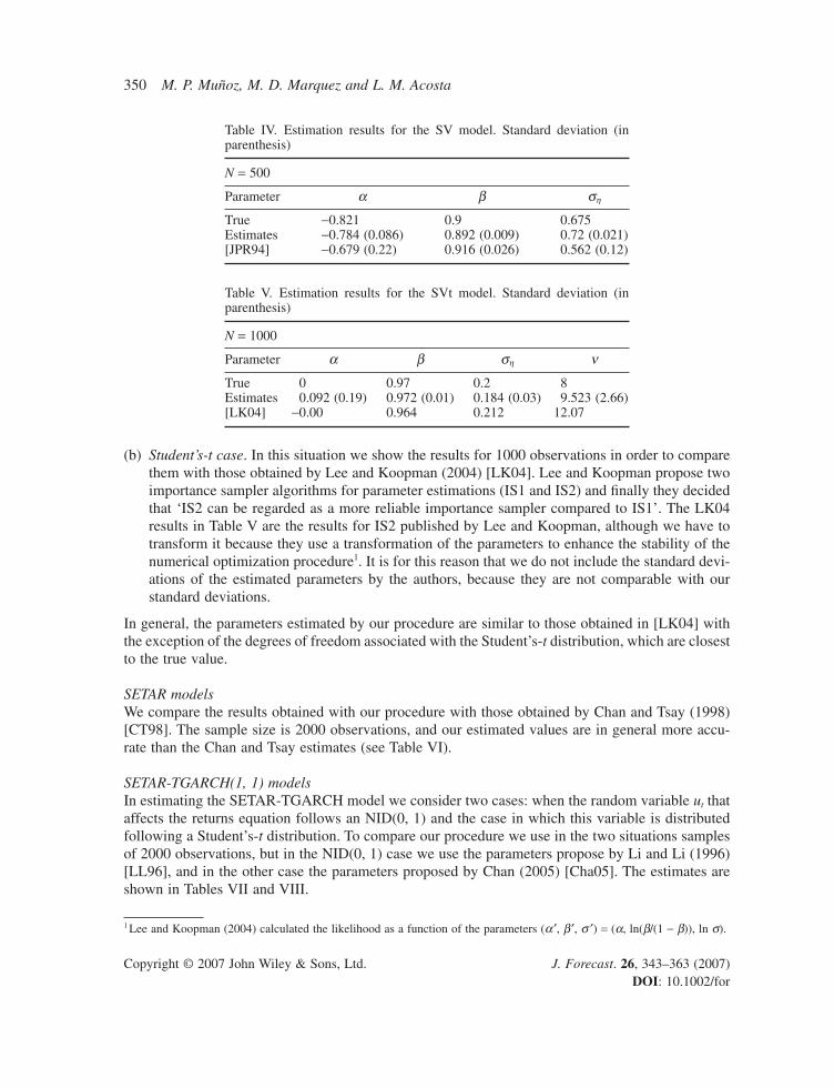
(a) NID(0, 1) case. Table IV shows the estimation results for 500 observations in order to comparethem with the results of the Bayes Estimator published by Jacquier et al. (1994) [JPR04]. Forall parameters estimated, our results are more accurate than those obtained in [JPR04]. Severalexplanations of these disagreements might be possible. One of them would be that the estima-tion procedures are different; we use our proposed SIRJ algorithm, whereas Jacquier et al. useda cyclic Metropolis algorithm to construct a Markov chain simulation tool. Another possiblecause of these discrepancies could be that the results of the SIRJ algorithm are based on M =10,000 particles and the Bayes estimator from Jacquier et al. is constructed using a drawsequence of length 4000 from the Markov chain constructed according to their algorithm anddiscarding the first 1500 draws, leaving a sequence of length 2500 to compute an estimate ofthe posterior mean. Maybe if they used a draw sequence of greater length the discrepancieswould be smaller.

Table II. References of results published

Model GARCHt SV SVt SETAR SETAR- SETAR- SETAR- SETAR-TGARCH TGARCHt THSV THSVt

Reference [BL98] [JPR94] [LK04] [CT98] [LL96] [Cha05] [SLL02] [SLL02]Bauwens and Jacquier Lee and Chan and Li and Li Chan So et al. So et al.

Lubrano et al. Koopman Tsay (1998) (1996) (2005) (2002) (2002)(1998) (1994) (2004)

Table III. Estimation results for the GARCH(1, 1)t model. Standarddeviation (in parenthesis)

N = 150

Parameter g0 g1 l1 n

True 0.1 0.4 0.4 5Estimates 0.14 (0.089) 0.415 (0.18) 0.32 (0.17) 6.24 (3.04)[BL98] 0.19 (0.10) 0.24 (0.12) 0.38 (0.38) 6.09 (2.49)



(b) Student’s-t case. In this situation we show the results for 1000 observations in order to comparethem with those obtained by Lee and Koopman (2004) [LK04]. Lee and Koopman propose twoimportance sampler algorithms for parameter estimations (IS1 and IS2) and finally they decidedthat ‘IS2 can be regarded as a more reliable importance sampler compared to IS1’. The LK04results in Table V are the results for IS2 published by Lee and Koopman, although we have totransform it because they use a transformation of the parameters to enhance the stability of thenumerical optimization procedure1. It is for this reason that we do not include the standard devi-ations of the estimated parameters by the authors, because they are not comparable with ourstandard deviations.

In general, the parameters estimated by our procedure are similar to those obtained in [LK04] withthe exception of the degrees of freedom associated with the Student’s-t distribution, which are closestto the true value.

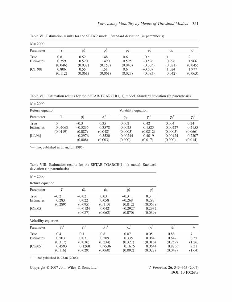
SETAR modelsWe compare the results obtained with our procedure with those obtained by Chan and Tsay (1998)[CT98]. The sample size is 2000 observations, and our estimated values are in general more accu-rate than the Chan and Tsay estimates (see Table VI).

SETAR-TGARCH(1, 1) modelsIn estimating the SETAR-TGARCH model we consider two cases: when the random variable ut thataffects the returns equation follows an NID(0, 1) and the case in which this variable is distributedfollowing a Student’s-t distribution. To compare our procedure we use in the two situations samplesof 2000 observations, but in the NID(0, 1) case we use the parameters propose by Li and Li (1996)[LL96], and in the other case the parameters proposed by Chan (2005) [Cha05]. The estimates areshown in Tables VII and VIII.

1 Lee and Koopman (2004) calculated the likelihood as a function of the parameters (a ′, b ′, s ′) = (a, ln(b/(1 − b)), ln s).

Table IV. Estimation results for the SV model. Standard deviation (inparenthesis)

N = 500

Parameter a b sh

True −0.821 0.9 0.675Estimates −0.784 (0.086) 0.892 (0.009) 0.72 (0.021)[JPR94] −0.679 (0.22) 0.916 (0.026) 0.562 (0.12)

Table V. Estimation results for the SVt model. Standard deviation (inparenthesis)

N = 1000

Parameter a b sh n

True 0 0.97 0.2 8Estimates 0.092 (0.19) 0.972 (0.01) 0.184 (0.03) 9.523 (2.66)[LK04] −0.00 0.964 0.212 12.07



Table VI. Estimation results for the SETAR model. Standard deviation (in parenthesis)

N = 2000

Parameter T f10 f 2

0 f11 f2

1 s0 s1

True 0.8 0.52 1.48 0.6 −0.6 1 2Estimates 0.759 0.520 1.490 0.595 −0.596 0.996 1.966

(0.046) (0.032) (0.157) (0.048) (0.063) (0.021) (0.045)[CT 98] 0.806 0.55 1.51 0.6 −0.607 1.024 1.977

(0.112) (0.061) (0.061) (0.027) (0.083) (0.042) (0.063)

Table VIII. Estimation results for the SETAR-TGARCH(1, 1)t model. Standarddeviation (in parenthesis)

N = 2000

Return equation

Parameter T f10 f2

0 f11 f2

1

True −0.2 −0.02 0.03 −0.3 0.3Estimates 0.283 0.022 0.058 −0.268 0.298

(0.289) (0.095) (0.113) (0.012) (0.063)[Cha05] — −0.0124 0.0421 −0.2927 0.2932

(0.087) (0.062) (0.070) (0.039)

Volatility equation

Parameter g 01 g 1

1 l 11 g 0

2 g 12 l1

2 n

True 0.4 0.1 0.8 0.07 0.05 0.88 7Estimates 0.503 0.071 0.509 0.335 0.064 0.647 6.35

(0.317) (0.036) (0.234) (0.327) (0.016) (0.259) (1.26)[Cha05] 0.4593 0.1260 0.7536 0.1676 0.0644 0.8256 7.31

(0.116) (0.029) (0.060) (0.092) (0.022) (0.048) (1.64)

‘—’, not published in Chan (2005).

Table VII. Estimation results for the SETAR-TGARCH(1, 1) model. Standard deviation (in parenthesis)

N = 2000

Return equation Volatility equation

Parameter T f11 f2

1 g 01 g 1

1 g 20 g 1

2

True 0 −0.3 0.35 0.002 0.42 0.004 0.24Estimates 0.02068 −0.3235 0.3578 0.0025 0.1525 0.00227 0.2155

(0.0119) (0.087) (0.048) (0.0005) (0.0812) (0.0005) (0.066)[LL96] — −0.2976 0.3520 0.00244 0.4019 0.00424 0.2307

(0.008) (0.003) (0.000) (0.017) (0.000) (0.014)

‘—’, not published in Li and Li (1996).



Depending on whether the error terms {ut} follow a Gaussian or a Student’s t distribution, twocases are considered:

(a) NID(0, 1) case. The reference model used by Li and Li [LL96] has some special features: theconstant term in the return equation f i

0 is equal to zero in both regimes and also l i0 = 0 in both

regimes. Our estimated values both for the return and volatility equations (see Table VII) arevery close to the true values, with the exception of g 1

1, for which our estimated values are notas accurate as those obtained in [LL96].

(b) Student’s-t case. From the results of Table VIII we can observe that the true value of each param-eter belongs to the 95% confidence interval obtained from our estimation, although the estimatesobtained by Chan (2005) are in general more accurate than ours. One possible reason of this dis-crepancy could be that the estimation procedure is very different of our algorithm. Chan’s esti-mates are based on the last 12,000 MCMC iterates (after a burn-in of 8000) from 100 replicationsof the model, and our estimation is based in the simplex method of Nelder and Mead (1965).

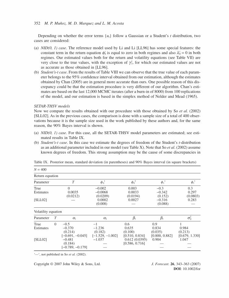
SETAR-THSV modelsNow we compare the results obtained with our procedure with those obtained by So et al. (2002)[SLL02]. As in the previous cases, the comparison is done with a sample size of a total of 400 obser-vations because it is the sample size used in the work published by these authors and, for the samereason, the 90% Bayes interval is shown.

(a) NID(0, 1) case. For this case, all the SETAR-THSV model parameters are estimated; see esti-mated results in Table IX.

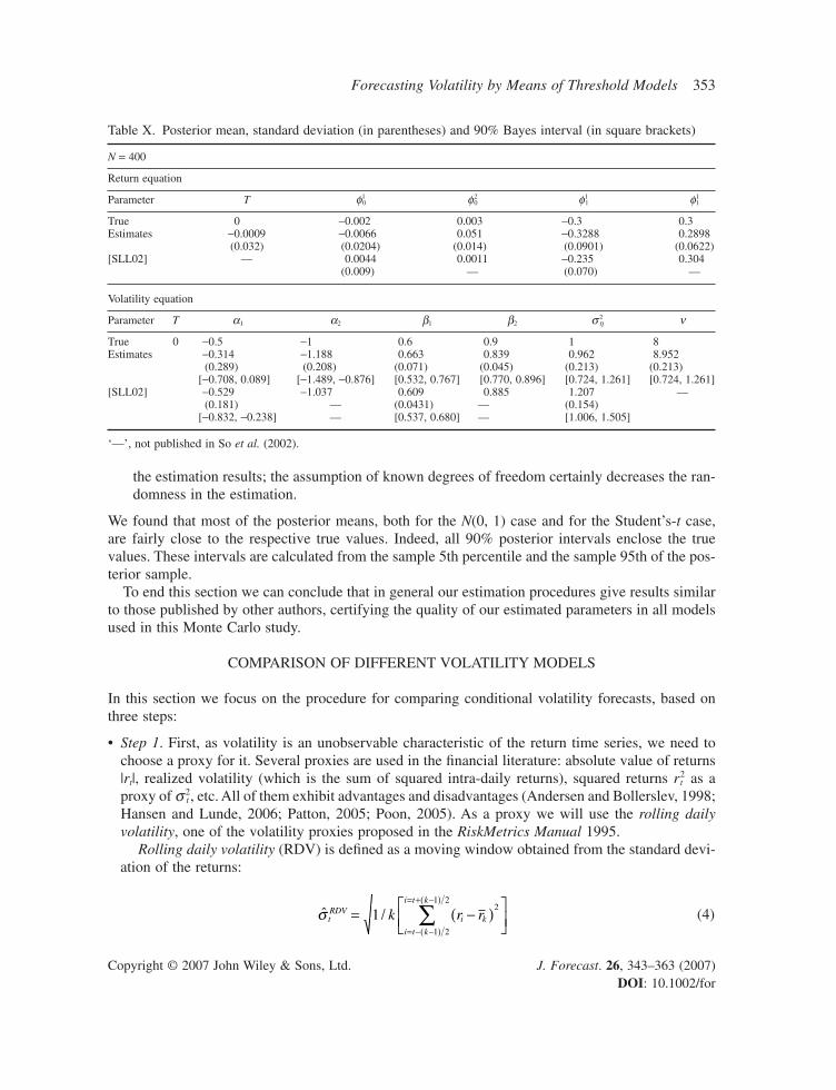
(b) Student’s-t case. In this case we estimate the degrees of freedom of the Student’s t-distributionas an additional parameter included in our model (see Table X). Note that So et al. (2002) assumeknown degrees of freedom. This strong assumption may be the cause of some discrepancies in

Table IX. Posterior mean, standard deviation (in parentheses) and 90% Bayes interval (in square brackets)

N = 400

Return equation

Parameter T f 01 f 0

2 f 11 f1

1

True 0 −0.002 0.003 −0.3 0.3Estimates 0.0035 −0.0068 0.0033 −0.342 0.297

(0.0212) (0.0209) (0.0194) (0.152) (0.0803)[SLL02] — 0.0002 0.0027 −0.316 0.283

(0.008) — (0.088) —

Volatility equation

Parameter T a1 a2 b1 b2 s 2h

True 0 −0.5 −1 0.6 0.9 1Estimates −0.370 −1.236 0.635 0.834 0.984

(0.214) (0.182) (0.100) (0.035) (0.213)[−0.691, −0.045] [−1.529, −1.002] [0.510, 0.834] [0.800, 0.882] [0.679, 1.330]

[SLL02] −0.481 −1.037 0.612 (0.0395) 0.904 1.047(0.184) — [0.586, 0.716] — —

[−0.789, −0.179] — — —

‘—’, not published in So et al. (2002).



the estimation results; the assumption of known degrees of freedom certainly decreases the ran-domness in the estimation.

We found that most of the posterior means, both for the N(0, 1) case and for the Student’s-t case,are fairly close to the respective true values. Indeed, all 90% posterior intervals enclose the truevalues. These intervals are calculated from the sample 5th percentile and the sample 95th of the pos-terior sample.

To end this section we can conclude that in general our estimation procedures give results similarto those published by other authors, certifying the quality of our estimated parameters in all modelsused in this Monte Carlo study.

COMPARISON OF DIFFERENT VOLATILITY MODELS

In this section we focus on the procedure for comparing conditional volatility forecasts, based onthree steps:

• Step 1. First, as volatility is an unobservable characteristic of the return time series, we need tochoose a proxy for it. Several proxies are used in the financial literature: absolute value of returns|rt|, realized volatility (which is the sum of squared intra-daily returns), squared returns r2

t as aproxy of s 2

t , etc. All of them exhibit advantages and disadvantages (Andersen and Bollerslev, 1998;Hansen and Lunde, 2006; Patton, 2005; Poon, 2005). As a proxy we will use the rolling dailyvolatility, one of the volatility proxies proposed in the RiskMetrics Manual 1995.

Rolling daily volatility (RDV) is defined as a moving window obtained from the standard devi-ation of the returns:

(4)ˆ /s tRDV

i k

i t k

i t k

k r r= −( )

= − −( )

= + −( )

∑12

1 2

1 2

Table X. Posterior mean, standard deviation (in parentheses) and 90% Bayes interval (in square brackets)

N = 400

Return equation

Parameter T f10 f2

0 f11 f1

1

True 0 −0.002 0.003 −0.3 0.3Estimates −0.0009 −0.0066 0.051 −0.3288 0.2898

(0.032) (0.0204) (0.014) (0.0901) (0.0622)[SLL02] — 0.0044 0.0011 −0.235 0.304

(0.009) — (0.070) —

Volatility equation

Parameter T a1 a2 b1 b2 s 2h n

True 0 −0.5 −1 0.6 0.9 1 8Estimates −0.314 −1.188 0.663 0.839 0.962 8.952

(0.289) (0.208) (0.071) (0.045) (0.213) (0.213)[−0.708, 0.089] [−1.489, −0.876] [0.532, 0.767] [0.770, 0.896] [0.724, 1.261] [0.724, 1.261]

[SLL02] −0.529 −1.037 0.609 0.885 1.207 —(0.181) — (0.0431) — (0.154)

[−0.832, −0.238] — [0.537, 0.680] — [1.006, 1.505]

‘—’, not published in So et al. (2002).



where k is the lag length of the rolling window, in days, and r–k is the sample mean of the k returnsused.

• Step 2. A loss function must then be chosen from among the loss functions used by several authors,in order to compare the goodness-of-fit of the one-step-ahead forecast obtained from one of thevolatility models and used in this paper to the rolling daily volatility defined by equation (4). Wepropose to use the following quadratic function:

(5)

where st+1/t is the one-step-ahead forecast obtained from the volatility model.

• Step 3. Finally, the out-of-sample predictive accuracy of different models is statistically testedusing Diebold and Mariano’s sign test (Diebold and Mariano, 1995) for comparing forecast errorsof different models. Following Poon (2005), let {s i

t+1/t}Nt=1 and {s j

t+1/t}Nt=1 be two sets of forecasts

for the volatility {st+1}Nt=1 from models i and j, respectively. The loss function defined in equation

(5) is used to calculate the loss differential as

(6)

This loss differential is simply the difference between the two forecast errors obtained from modelsi and j, respectively. In this case, we test the null hypothesis:

(7)

Assuming that dt ∼ i.i.d., then the test statistic is

(8)

Following Diebold and Mariano (1995), the large sample Studentized version of an exact finitesample test, the sign test, is asymptotically normal:

(9)

EMPIRICAL RESULTS

The data consist of daily closing values for two stock indices: Standard & Poor’s 500 Index andIBEX 35, the official index returns of the Spanish Stock Exchange continuous market. All of thedata were taken from Reuters (www.reuters.es). We considered, following the conventionalapproach, the daily stock-return time series in each case:

SS N

NNa = − ( )0 5

0 250 1

..

~ ,

S I d I dd

t tt

t

N

= ( ) ( ) =>

+ +=∑ where

if

otherwise

1 0

01

H E d

vs H E dt

t

0

1

0

0

:

. :

( ) =( ) ≠

dt tRDV

t ti

tRDV

t tj

+ + + + += ( ) − ( )( ) − ( ) − ( )( )1 12

1

2 2

12

1

2 2

ˆ ˆ ˆ ˆs s s s

L tRDV

t t tRDV

t tˆ , ˆ ˆ ˆs s s s+ + + +( ) = ( ) − ( )( )1 1 12

12 2



• The S&P 500 (S&P) composite index returns spans from October 10, 1990 through December 3,2003 (3085 observations). The first 2785 observations are used for parameter estimation and thelast 300 for one-step-ahead forecasting.

• IBEX 35 (IBEX) is the official index returns of the Spanish Stock Exchange continuous market.This data set consists of 3932 observations of IBEX and spans from January 2, 1990 through May10, 2005. The first 3539 observations are used in the estimation process and 393 in one-step-aheadforecasting.

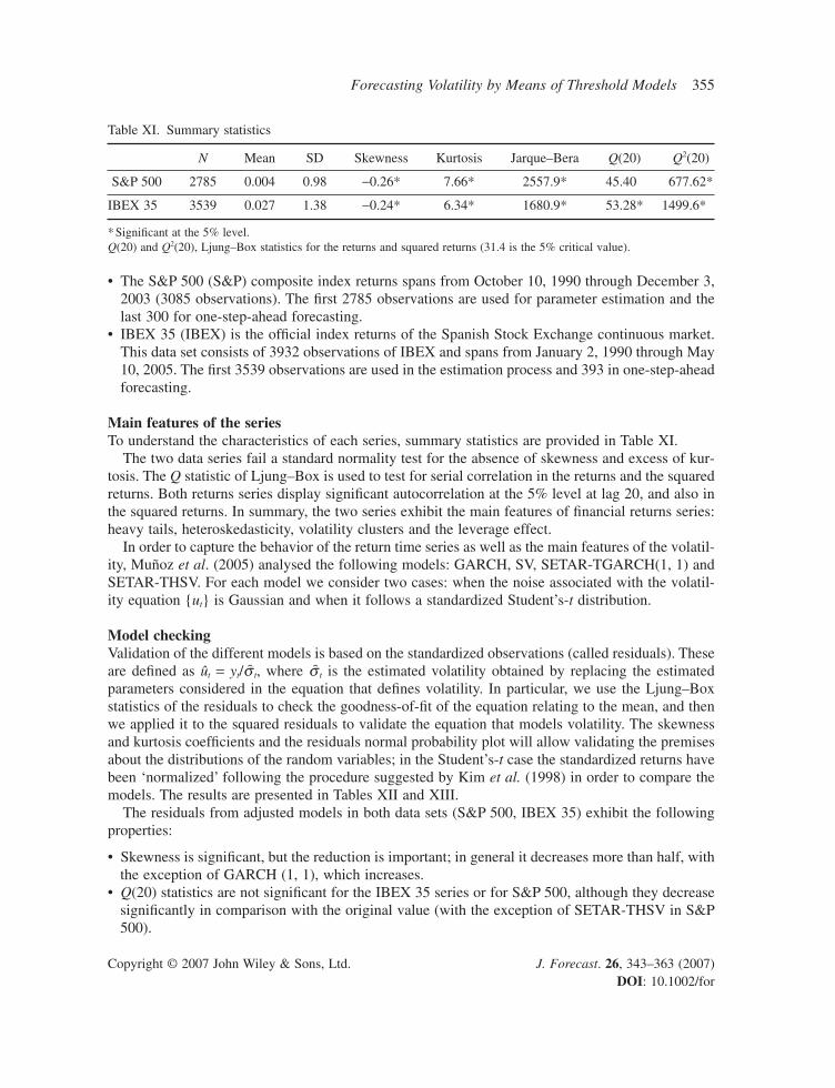
Main features of the seriesTo understand the characteristics of each series, summary statistics are provided in Table XI.

The two data series fail a standard normality test for the absence of skewness and excess of kur-tosis. The Q statistic of Ljung–Box is used to test for serial correlation in the returns and the squaredreturns. Both returns series display significant autocorrelation at the 5% level at lag 20, and also inthe squared returns. In summary, the two series exhibit the main features of financial returns series:heavy tails, heteroskedasticity, volatility clusters and the leverage effect.

In order to capture the behavior of the return time series as well as the main features of the volatil-ity, Muñoz et al. (2005) analysed the following models: GARCH, SV, SETAR-TGARCH(1, 1) andSETAR-THSV. For each model we consider two cases: when the noise associated with the volatil-ity equation {ut} is Gaussian and when it follows a standardized Student’s-t distribution.

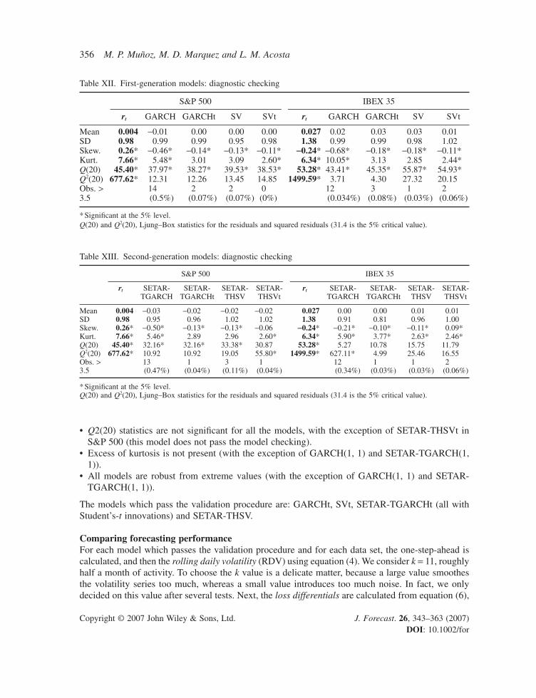
Model checkingValidation of the different models is based on the standardized observations (called residuals). Theseare defined as ut = yt/s�t, where s�t is the estimated volatility obtained by replacing the estimatedparameters considered in the equation that defines volatility. In particular, we use the Ljung–Boxstatistics of the residuals to check the goodness-of-fit of the equation relating to the mean, and thenwe applied it to the squared residuals to validate the equation that models volatility. The skewnessand kurtosis coefficients and the residuals normal probability plot will allow validating the premisesabout the distributions of the random variables; in the Student’s-t case the standardized returns havebeen ‘normalized’ following the procedure suggested by Kim et al. (1998) in order to compare themodels. The results are presented in Tables XII and XIII.

The residuals from adjusted models in both data sets (S&P 500, IBEX 35) exhibit the followingproperties:

• Skewness is significant, but the reduction is important; in general it decreases more than half, withthe exception of GARCH (1, 1), which increases.

• Q(20) statistics are not significant for the IBEX 35 series or for S&P 500, although they decreasesignificantly in comparison with the original value (with the exception of SETAR-THSV in S&P500).

Table XI. Summary statistics

N Mean SD Skewness Kurtosis Jarque–Bera Q(20) Q2(20)

S&P 500 2785 0.004 0.98 −0.26* 7.66* 2557.9* 45.40 677.62*

IBEX 35 3539 0.027 1.38 −0.24* 6.34* 1680.9* 53.28* 1499.6*

* Significant at the 5% level.Q(20) and Q2(20), Ljung–Box statistics for the returns and squared returns (31.4 is the 5% critical value).



• Q2(20) statistics are not significant for all the models, with the exception of SETAR-THSVt inS&P 500 (this model does not pass the model checking).

• Excess of kurtosis is not present (with the exception of GARCH(1, 1) and SETAR-TGARCH(1,1)).

• All models are robust from extreme values (with the exception of GARCH(1, 1) and SETAR-TGARCH(1, 1)).

The models which pass the validation procedure are: GARCHt, SVt, SETAR-TGARCHt (all withStudent’s-t innovations) and SETAR-THSV.

Comparing forecasting performanceFor each model which passes the validation procedure and for each data set, the one-step-ahead iscalculated, and then the rolling daily volatility (RDV) using equation (4). We consider k = 11, roughlyhalf a month of activity. To choose the k value is a delicate matter, because a large value smoothesthe volatility series too much, whereas a small value introduces too much noise. In fact, we onlydecided on this value after several tests. Next, the loss differentials are calculated from equation (6),

Table XII. First-generation models: diagnostic checking

S&P 500 IBEX 35

rt GARCH GARCHt SV SVt rt GARCH GARCHt SV SVt

Mean 0.004 −0.01 0.00 0.00 0.00 0.027 0.02 0.03 0.03 0.01SD 0.98 0.99 0.99 0.95 0.98 1.38 0.99 0.99 0.98 1.02Skew. 0.26* −0.46* −0.14* −0.13* −0.11* -0.24* −0.68* −0.18* −0.18* −0.11*Kurt. 7.66* 5.48* 3.01 3.09 2.60* 6.34* 10.05* 3.13 2.85 2.44*Q(20) 45.40* 37.97* 38.27* 39.53* 38.53* 53.28* 43.41* 45.35* 55.87* 54.93*Q2(20) 677.62* 12.31 12.26 13.45 14.85 1499.59* 3.71 4.30 27.32 20.15Obs. > 14 2 2 0 12 3 1 23.5 (0.5%) (0.07%) (0.07%) (0%) (0.034%) (0.08%) (0.03%) (0.06%)

* Significant at the 5% level.Q(20) and Q2(20), Ljung–Box statistics for the residuals and squared residuals (31.4 is the 5% critical value).

Table XIII. Second-generation models: diagnostic checking

S&P 500 IBEX 35

rt SETAR- SETAR- SETAR- SETAR- rt SETAR- SETAR- SETAR- SETAR-TGARCH TGARCHt THSV THSVt TGARCH TGARCHt THSV THSVt

Mean 0.004 −0.03 −0.02 −0.02 −0.02 0.027 0.00 0.00 0.01 0.01SD 0.98 0.95 0.96 1.02 1.02 1.38 0.91 0.81 0.96 1.00Skew. 0.26* −0.50* −0.13* −0.13* −0.06 -0.24* −0.21* −0.10* −0.11* 0.09*Kurt. 7.66* 5.46* 2.89 2.96 2.60* 6.34* 5.90* 3.77* 2.63* 2.46*Q(20) 45.40* 32.16* 32.16* 33.38* 30.87 53.28* 5.27 10.78 15.75 11.79Q2(20) 677.62* 10.92 10.92 19.05 55.80* 1499.59* 627.11* 4.99 25.46 16.55Obs. > 13 1 3 1 12 1 1 23.5 (0.47%) (0.04%) (0.11%) (0.04%) (0.34%) (0.03%) (0.03%) (0.06%)

* Significant at the 5% level.Q(20) and Q2(20), Ljung–Box statistics for the residuals and squared residuals (31.4 is the 5% critical value).



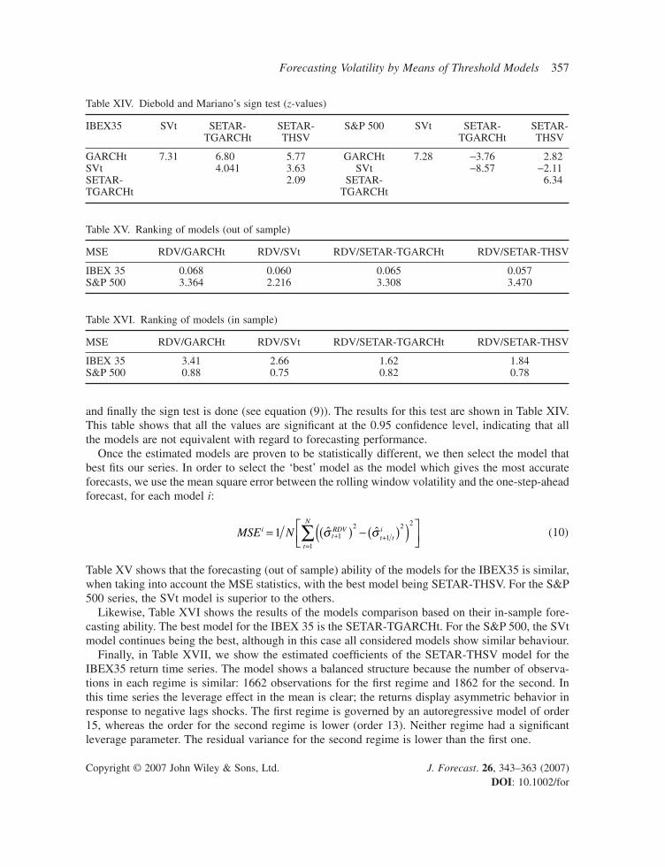
and finally the sign test is done (see equation (9)). The results for this test are shown in Table XIV.This table shows that all the values are significant at the 0.95 confidence level, indicating that allthe models are not equivalent with regard to forecasting performance.

Once the estimated models are proven to be statistically different, we then select the model thatbest fits our series. In order to select the ‘best’ model as the model which gives the most accurateforecasts, we use the mean square error between the rolling window volatility and the one-step-aheadforecast, for each model i:

(10)

Table XV shows that the forecasting (out of sample) ability of the models for the IBEX35 is similar,when taking into account the MSE statistics, with the best model being SETAR-THSV. For the S&P500 series, the SVt model is superior to the others.

Likewise, Table XVI shows the results of the models comparison based on their in-sample fore-casting ability. The best model for the IBEX 35 is the SETAR-TGARCHt. For the S&P 500, the SVtmodel continues being the best, although in this case all considered models show similar behaviour.

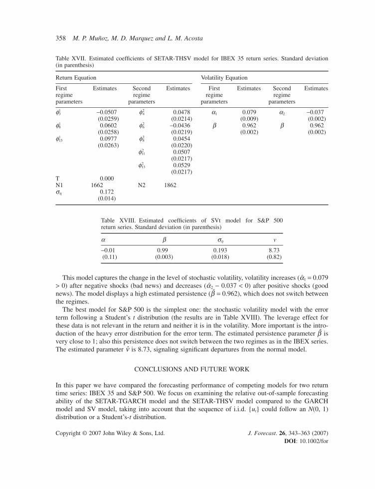
Finally, in Table XVII, we show the estimated coefficients of the SETAR-THSV model for theIBEX35 return time series. The model shows a balanced structure because the number of observa-tions in each regime is similar: 1662 observations for the first regime and 1862 for the second. Inthis time series the leverage effect in the mean is clear; the returns display asymmetric behavior inresponse to negative lags shocks. The first regime is governed by an autoregressive model of order15, whereas the order for the second regime is lower (order 13). Neither regime had a significantleverage parameter. The residual variance for the second regime is lower than the first one.

MSE NitRDV

t ti

t

N

= ( ) − ( )( )

+ +=∑1 1

2

1

2 2

1

ˆ ˆs s

Table XIV. Diebold and Mariano’s sign test (z-values)

IBEX35 SVt SETAR- SETAR- S&P 500 SVt SETAR- SETAR-TGARCHt THSV TGARCHt THSV

GARCHt 7.31 6.80 5.77 GARCHt 7.28 −3.76 2.82SVt 4.041 3.63 SVt −8.57 −2.11SETAR- 2.09 SETAR- 6.34TGARCHt TGARCHt

Table XV. Ranking of models (out of sample)

MSE RDV/GARCHt RDV/SVt RDV/SETAR-TGARCHt RDV/SETAR-THSV

IBEX 35 0.068 0.060 0.065 0.057S&P 500 3.364 2.216 3.308 3.470

Table XVI. Ranking of models (in sample)

MSE RDV/GARCHt RDV/SVt RDV/SETAR-TGARCHt RDV/SETAR-THSV

IBEX 35 3.41 2.66 1.62 1.84S&P 500 0.88 0.75 0.82 0.78



This model captures the change in the level of stochastic volatility, volatility increases (a�1 = 0.079> 0) after negative shocks (bad news) and decreases (a�2 − 0.037 < 0) after positive shocks (goodnews). The model displays a high estimated persistence (b = 0.962), which does not switch betweenthe regimes.

The best model for S&P 500 is the simplest one: the stochastic volatility model with the errorterm following a Student’s t distribution (the results are in Table XVIII). The leverage effect forthese data is not relevant in the return and neither it is in the volatility. More important is the intro-duction of the heavy error distribution for the error term. The estimated persistence parameter b isvery close to 1; also this persistence does not switch between the two regimes as in the IBEX series.The estimated parameter n is 8.73, signaling significant departures from the normal model.

CONCLUSIONS AND FUTURE WORK

In this paper we have compared the forecasting performance of competing models for two returntime series: IBEX 35 and S&P 500. We focus on examining the relative out-of-sample forecastingability of the SETAR-TGARCH model and the SETAR-THSV model compared to the GARCHmodel and SV model, taking into account that the sequence of i.i.d. {ut} could follow an N(0, 1)distribution or a Student’s-t distribution.

Table XVII. Estimated coefficients of SETAR-THSV model for IBEX 35 return series. Standard deviation (in parenthesis)

Return Equation Volatility Equation

First Estimates Second Estimates First Estimates Second Estimatesregime regime regime regimeparameters parameters parameters parameters

f13 −0.0507 f2

4 0.0478 a1 0.079 a2 −0.037(0.0259) (0.0214) (0.009) (0.002)

f18 0.0602 f2

6 −0.0436 b 0.962 b 0.962(0.0258) (0.0219) (0.002) (0.002)

f115 0.0977 f2

8 0.0454(0.0263) (0.0220)

f211 0.0507

(0.0217)f2

13 0.0529(0.0217)

T 0.000N1 1662 N2 1862sh 0.172

(0.014)

Table XVIII. Estimated coefficients of SVt model for S&P 500 return series. Standard deviation (in parenthesis)

a b sh v

−0.01 0.99 0.193 8.73(0.11) (0.003) (0.018) (0.82)



We tested the quality of the estimation of the different procedures used in this paper by means ofa Monte Carlo study and selected the parameters in accordance with previous models published inthe financial literature. In general our estimation results are similar to the ones published in thosepapers.

We fit the first- and second-generation models listed in Table I for each return time series. Themodels which pass the validation procedure are: GARCHt, SVt, SETAR-TGARCHt (all withStudent’s-t innovations) and SETAR-THSV. We observe that SETAR-THSVt dominates all ofmodels studied in capturing asymmetries.

We compared the models in order to obtain the best model for forecasting. We have used as avolatility proxy the rolling daily volatility and a loss function. This is an important decision becausethe quality of the comparison greatly depends on the choice of the proxies and the definition of theloss function.

The results of the comparison yield a different model for each time series. The SETAR-THSVt isthe best model for the IBEX35 returns. This time series, which includes leverage effects on the mean,the introduction of threshold in the mean and variance model equations, produces more accurate pre-dictions. Table XVII shows an asymmetric response. In this table we can observe that this modelcapture the changes in the level in stochastic volatility, which increases after negative shocks anddecreases after positive shocks.

On the other hand, the S&P 500 returns series the leverage in the mean is not important; the SVtmodel is then flexible enough to beat the threshold models, and the best model is the simplest one.The leverage effect is not relevant in the return; neither it is in the volatility. Finally, the introduc-tion of the Student’s-t distribution is important, the degrees of freedom being 8.73 (0.82).

Finally, empirical evidence applied to eight international financial market indices, including theG-7 countries, supports the hypothesis of threshold nonlinearity in both the mean and also in thevolatility (Chen et al., 2005). Our results are in line with this study in the sense that if the leverageeffect is not present in a return time series, the fit of sophisticated second-generation models is unnec-essary in forecasting. Further investigation, however, is needed.

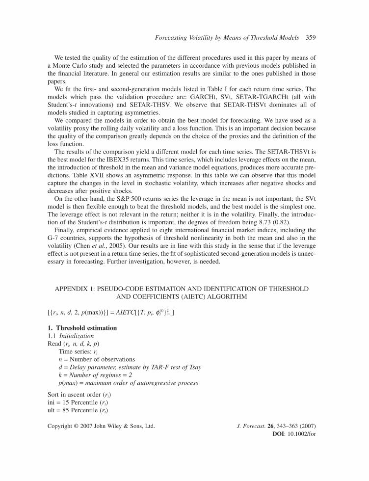
APPENDIX 1: PSEUDO-CODE ESTIMATION AND IDENTIFICATION OF THRESHOLDAND COEFFICIENTS (AIETC) ALGORITHM

[{rt, n, d, 2, p(max))}] = AIETC[{T, pi, fl(i)}2

i=1]

1. Threshold estimation1.1 InitializationRead (rt, n, d, k, p)

Time series: rt

n = Number of observationsd = Delay parameter, estimate by TAR-F test of Tsayk = Number of regimes = 2p(max) = maximum order of autoregressive process

Sort in ascent order (rt)ini = 15 Percentile (rt)ult = 85 Percentile (rt)



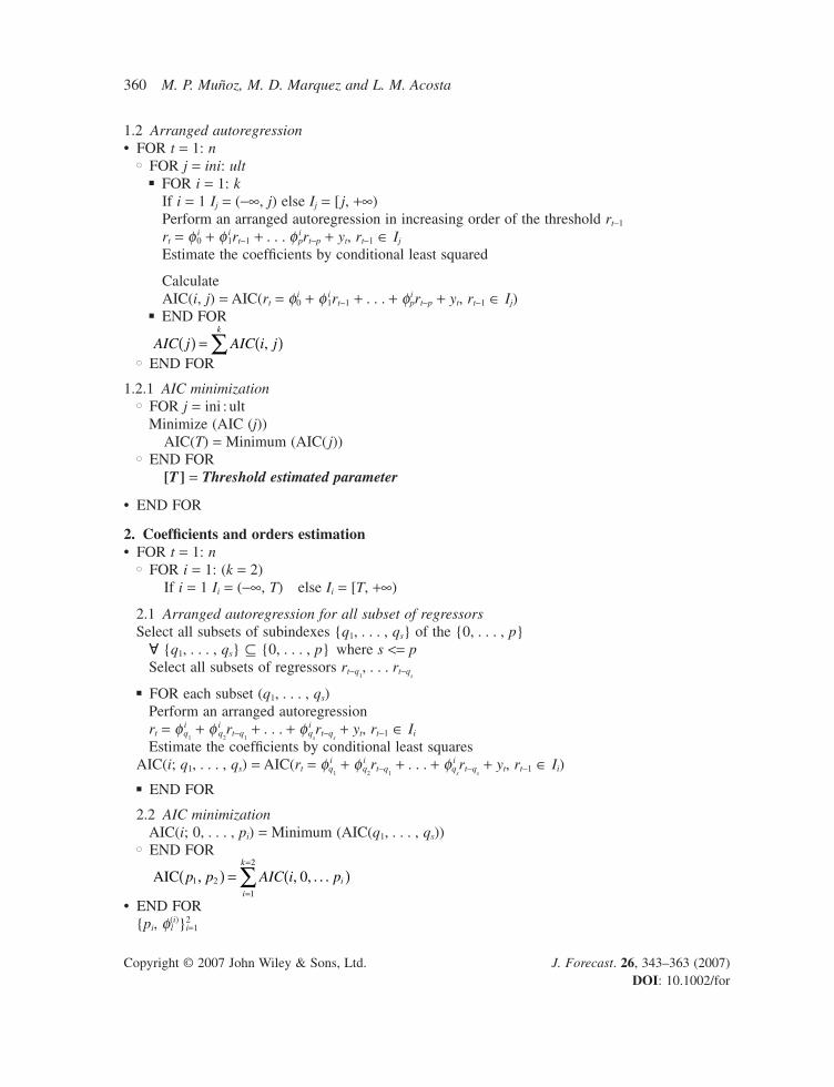
1.2 Arranged autoregression• FOR t = 1: n

� FOR j = ini: ult� FOR i = 1: k

If i = 1 Ij = (−∞, j) else Ij = [ j, +∞)Perform an arranged autoregression in increasing order of the threshold rt−1

rt = f i0 + f i

1rt−1 + . . . f iprt−p + yt, rt−1 ∈ Ij

Estimate the coefficients by conditional least squared

CalculateAIC(i, j) = AIC(rt = fi

0 + f i1rt−1 + . . . + f i

prt−p + yt, rt−1 ∈ Ij)� END FOR

� END FOR

1.2.1 AIC minimization� FOR j = ini : ult

Minimize (AIC (j))AIC(T) = Minimum (AIC( j))

� END FOR[T] = Threshold estimated parameter

• END FOR

2. Coefficients and orders estimation• FOR t = 1: n

� FOR i = 1: (k = 2)If i = 1 Ii = (−∞, T) else Ii = [T, +∞)

2.1 Arranged autoregression for all subset of regressorsSelect all subsets of subindexes {q1, . . . , qs} of the {0, . . . , p}

� {q1, . . . , qs} � {0, . . . , p} where s <= pSelect all subsets of regressors rt−q

1, . . . rt−q

s

� FOR each subset (q1, . . . , qs)Perform an arranged autoregressionrt = f i

q1

+ f iq

2rt−q

1+ . . . + f i

qsrt−q

s+ yt, rt−1 ∈ Ii

Estimate the coefficients by conditional least squaresAIC(i; q1, . . . , qs) = AIC(rt = f i

q1

+ f iq

2rt−q

1+ . . . + f i

qsrt−q

s+ yt, rt−1 ∈ Ii)

� END FOR

2.2 AIC minimizationAIC(i; 0, . . . , pi) = Minimum (AIC(q1, . . . , qs))

� END FOR

• END FOR{pi, fl

(i)}2i=1

AIC p p AIC i pi

i

k

1 2

1

2

0, , , . . .( ) = ( )=

=

∑

AIC j AIC i jk

( ) = ( )∑ ,



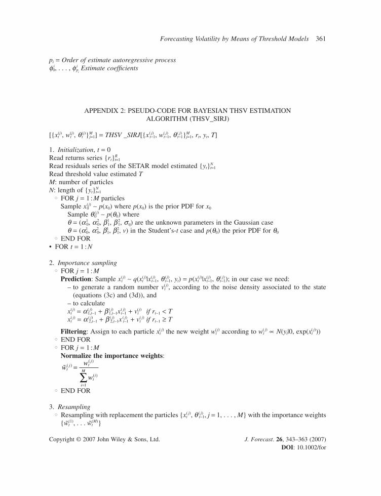
pi = Order of estimate autoregressive processf i

0, . . . , f ip

iEstimate coefficients

APPENDIX 2: PSEUDO-CODE FOR BAYESIAN THSV ESTIMATION ALGORITHM (THSV_SIRJ)

[{xt(j), wt

(j), qt(j)}M

j=1] = THSV _SIRJ[{x( j)t−1, w( j)

t−1, q ( j)t−1}M

j=1, rt, yt, T]

1. Initialization, t = 0Read returns series {rt}R

t=1

Read residuals series of the SETAR model estimated {yt}Nt=1

Read threshold value estimated TM: number of particlesN: length of {yt}N

t=1� FOR j = 1 : M particles

Sample x0(j) ∼ p(x0) where p(x0) is the prior PDF for x0

Sample q0(j) ∼ p(q0) where

q = (a10, a2

0, b11, b 2

1, sh) are the unknown parameters in the Gaussian caseq = (a1

0, a20, b1

1, b21, v) in the Student’s-t case and p(q0) the prior PDF for q0

� END FOR• FOR t = 1 : N

2. Importance sampling� FOR j = 1 : M

Prediction: Sample xt(j) ∼ q(xt

(j)|x(j)t−1, q (j)

t−1, yt) = p(xt(j)|x(j)

t−1, q ( j)t−1); in our case we need:

– to generate a random number vt(j), according to the noise density associated to the state

(equations (3c) and (3d)), and– to calculatext

(j) = a( j)1,t−1 + b ( j)

1,t−1x( j)t−1 + vt

(j) if rt−1 < Txt

( j) = a ( j)2,t−1 + b ( j)

2,t−1x ( j)t−1 + vt

( j) if rt−1 ≥ T

Filtering: Assign to each particle xt( j) the new weight wt

(j) according to wt( j) ∝ N(yt|0, exp(xt

( j)))� END FOR� FOR j = 1 : M

Normalize the importance weights:

� END FOR

3. Resampling� Resampling with replacement the particles {xt

( j), q ( j)t−1, j = 1, . . . , M} with the importance weights

{wt(1), . . . wt

(M)}

ww

wt

j tj

ti

i

M( )

( )

( )

=

=

∑1



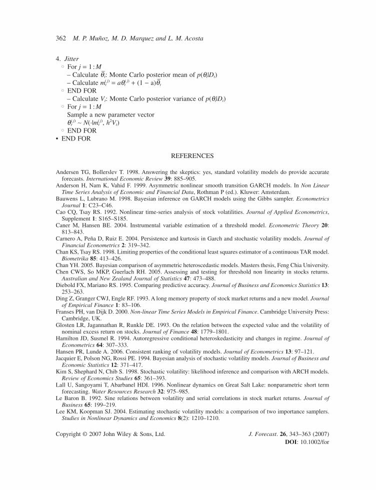
4. Jitter� For j = 1 : M

– Calculate q–t: Monte Carlo posterior mean of p(qt|Dt)– Calculate mt

( j) = aqt( j) + (1 − a)q–t

� END FOR– Calculate Vt: Monte Carlo posterior variance of p(qt|Dt)

� For j = 1 : MSample a new parameter vectorq t

( j) ∼ N(·|mt( j), h2Vt)

� END FOR• END FOR

REFERENCES

Andersen TG, Bollerslev T. 1998. Answering the skeptics: yes, standard volatility models do provide accurateforecasts. International Economic Review 39: 885–905.

Anderson H, Nam K, Vahid F. 1999. Asymmetric nonlinear smooth transition GARCH models. In Non LinearTime Series Analysis of Economic and Financial Data, Rothman P (ed.). Kluwer: Amsterdam.

Bauwens L, Lubrano M. 1998. Bayesian inference on GARCH models using the Gibbs sampler. EconometricsJournal 1: C23–C46.

Cao CQ, Tsay RS. 1992. Nonlinear time-series analysis of stock volatilities. Journal of Applied Econometrics,Supplement 1: S165–S185.

Caner M, Hansen BE. 2004. Instrumental variable estimation of a threshold model. Econometric Theory 20:813–843.

Carnero A, Peña D, Ruiz E. 2004. Persistence and kurtosis in Garch and stochastic volatility models. Journal ofFinancial Econometrics 2: 319–342.

Chan KS, Tsay RS. 1998. Limiting properties of the conditional least squares estimator of a continuous TAR model.Biometrika 85: 413–426.

Chan YH. 2005. Bayesian comparison of asymmetric heteroscedastic models. Masters thesis, Feng Chia University.Chen CWS, So MKP, Guerlach RH. 2005. Assessing and testing for threshold non linearity in stocks returns.

Australian and New Zealand Journal of Statistics 47: 473–488.Diebold FX, Mariano RS. 1995. Comparing predictive accuracy. Journal of Business and Economics Statistics 13:

253–263.Ding Z, Granger CWJ, Engle RF. 1993. A long memory property of stock market returns and a new model. Journal

of Empirical Finance 1: 83–106.Franses PH, van Dijk D. 2000. Non-linear Time Series Models in Empirical Finance. Cambridge University Press:

Cambridge, UK.Glosten LR, Jagannathan R, Runkle DE. 1993. On the relation between the expected value and the volatility of

nominal excess return on stocks. Journal of Finance 48: 1779–1801.Hamilton JD, Susmel R. 1994. Autoregressive conditional heteroskedasticity and changes in regime. Journal of

Econometrics 64: 307–333.Hansen PR, Lunde A. 2006. Consistent ranking of volatility models. Journal of Econometrics 13: 97–121.Jacquier E, Polson NG, Rossi PE. 1994. Bayesian analysis of stochastic volatility models. Journal of Business and

Economic Statistics 12: 371–417.Kim S, Shephard N, Chib S. 1998. Stochastic volatility: likelihood inference and comparison with ARCH models.

Review of Economics Studies 65: 361–393.Lall U, Sangoyami T, Abarbanel HDI. 1996. Nonlinear dynamics on Great Salt Lake: nonparametric short term

forecasting. Water Resources Research 32: 975–985.Le Baron B. 1992. Sine relations between volatility and serial correlations in stock market returns. Journal of

Business 65: 199–219.Lee KM, Koopman SJ. 2004. Estimating stochastic volatility models: a comparison of two importance samplers.

Studies in Nonlinear Dynamics and Economics 8(2): 1210–1210.



Lewis PAW, Ray BK. 1997. Modelling long-range dependence, nonlinearity and periodic phenomena in sea surfacetemperature using TSMARS. Journal of the American Statistical Association 92: 881–893.

Li CW, Li WK. 1996. On a double-threshold autoregressive heteroscedastic time series models. Journal of AppliedEconometrics 11: 253–274.

Li WK, Lam K. 1995. Modelling the asymmetry in stock returns by a threshold ARCH model. Statistician 44:333–341.

Liu JS, Chen R. 1998. Sequential Monte Carlo methods for dynamic systems. Journal of the American StatisticalAssociation 93: 1032–1044.

Loudon GF, Watt WH, Yadav PK. 2000. An empirical analysis of alternative parametric ARCH models. Journalof Applied Econometrics 15: 117–136.

Márquez MD. 2002. Modelo SETAR aplicado a la volatilidad de la rentabilidad de las acciones: algoritmos parasu identificación. PhD dissertation. Universitat Politècnica de Catalunya, Spain. http://www.tdx.cesca.es/TDX-0109103-175045/index_cs.html [1 September 2002].

Muñoz MP, Márquez MD, Martí Recober M, Villazón C, Acosta L. 2004. Stochastic volatility and TAR-GARCHmodels: evaluation based on simulations and financial time series. In Proceedings of COMPSTAT 2004. Physica-Verlag/Springer (CD-ROM).

Muñoz MP, Márquez MD, Martí Recober M, Villazón C. 2005. A walk through non-linear models in financialseries. In 3rd World Conference on Computational Statistics and Data Analysis, Cyprus.

Nelder JA, Mead R. 1965. A simplex method for function minimization. Computer Journal 7: 308–315.Patton AJ. 2005. Volatility forecast evaluation and comparison using imperfect volatility proxies. In Econometric

Society 2005 World Congress.Poon SH. 2005. A Practical Guide to Forecasting Financial Market Volatility. Wiley: New York.Poon SH, Granger C. 2003. Forecasting financial market volatility: a review. Journal of Economic Literature 41:

478–539.Saei A. 2004. Threshold models with correlated random components. S3RI Methodology Working Papers, M04/07.

Southampton Statistical Sciences Research Institute, Southampton, UK.So MP, Li WK, Lam K. 2002. A threshold stochastic volatility. Journal of Forecasting 21: 473–500.Taylor SJ. 2005. Asset Price Dynamics, Volatility, and Prediction. Princeton University Press: Princeton, NJ.Tong H. 1990. Non-linear Time Series: A Dynamical System Approach. Oxford University Press: Oxford.Tsay RS. 1989. Testing and modelling threshold autoregressive processes. Journal of the American Statistical

Association 84: 231–240.Tsay RS. 2005. Analysis of Financial Time Series (2nd edn). Wiley–Interscience: Hoboken NJ.Zakoian JM. 1994. Threshold heteroscedastic models. Journal of Economic Dynamics and Control 18: 931–955.

Authors’ biographies:M. Pilar Munoz is an Associate Professor of Statistics in the Department of Statistics and Operations Research atthe Technical University of Catalonia (UPC). The author has a degree in Mathematics from the UniversitatAutònoma de Barcelona (1979) and a PhD in Computer Science from UPC (1988). Areas of expertise are time seriesanalysis, financial time series, nonlinear time series models, Bayesian estimation, and computational statistics.

M. Dolores Márquez is an Associate Professor of Statistics in the Department of Business Economics, Univer-sitat Autònoma de Barcelona (UAB). The author has a degree in Mathematics from the UAB (1989) and a PhDin Mathematics from the Universitat Politècnica de Catalunya (2002). Areas of expertise are financial time series,nonlinear time series modes, TAR and stochastic volatility models.

Lesly M. Acosta is a PhD student in Statistics at the Universitat Politècnica de Catalunya (UPC). The author hasa Bachelor of Science in Mathematics (1990) from the University of Texas at El Paso (UTEP), and a Master ofScience in Statistics (1992) from UTEP. Areas of research are state and parameter estimation for nonlinear andpossibly non-stationary non-Gaussian time series models via particle filters, and application to stochastic volatil-ity type models.

Authors’ addresses:M. Pilar Muñoz and Lesly M. Acosta, Department of Statistics and Operations Research, Technical Universityof Catalonia, North Campus—C5, Jordi Girona 1–3, 08034 Barcelona, Spain.

M. Dolores Márquez, Department of Business Economics, Autonomous University of Barcelona, CampusSabadell, Emprius 2, 08202 Sabadell, Barcelona, Spain.

forecasting volatility by means of threshold models

Documents