forecasting the term structure of interest rates with potentially … · 2016-11-21 · forecasting...

Forecasting the Term Structure of Interest Rates with

Potentially Misspecified Models∗

Yunjong Eo†

University of Sydney

Kyu Ho Kang‡

Korea University

August 2016

Abstract

This paper assesses the predictive gains of the pooling method in yield curve pre-diction. We consider three individual yield curve prediction models: the dynamicNelson-Siegel model (DNS), the arbitrage-free Nelson-Siegel model, and the randomwalk (RW) model as a benchmark. Despite the popularity of these three frameworks,none of them dominates the others across all maturities and forecast horizons. Thisfact indicates that the models are potentially misspecified. We investigate whethercombining the possibly misspecified models in a linear form and in a Markov-switchingmixture helps improve predictive accuracy. To do this, we evaluate the out-of-sampleforecasts of the pooled models compared to the individual models. In terms of densityprediction, the pooled model of the DNS and RW models consistently outperforms theindividual models regardless of maturities and forecast horizons. Our findings providestrong evidence that the pooling method can be a better option than selecting oneof the alternative models. We also find that the RW model has been important inimproving the forecasting accuracy since 2009.

JEL classification: G12, C11, F37Keywords: Model combination, Markov-switching mixture, Dynamic Nelson-Siegel,Affine term structure model

∗We thank Gianni Amisano, Graham Elliott, Helmut Lutkepohl, James Morley, Tara Sinclair, and seminarand conference participants at Texas A&M University, the Federal Reserve Bank of Dallas, the Reserve Bankof New Zealand, University of California, Riverside, Hitotsubashi University, the Bank of Korea, the Societyfor Nonlinear Dynamics and Econometrics Conference, Recent Developments in Financial Econometricsand Applications, EFaB@Bayes 250 Workshop, and Econometric Society Australasian Meeting for usefulfeedback. All remaining errors are our own.

†School of Economics, University of Sydney, NSW 2006, Australia; Tel: +61 2 9351 3075; Email: [email protected]

‡Department of Economics, Korea University, Seoul, South Korea, 136-701; Tel: +82 2 3290 5132; Email:[email protected]

1 Introduction

Forecasting the yield curve is extremely important for bond portfolio risk management,

monetary policy, and business cycle analysis. In the previous literature, three classes

of yield curve prediction models have been widely used. One is the arbitrage-free affine

term structure model, which is a theoretical bond pricing approach.1 This approach

provides many economically interpretable outcomes such as term premium and term

structure of real interest rates. Despite its flexibility and microfoundation, this class

of models is known to be difficult to estimate because of its nonlinearity and irregular

likelihood surface.

Another approach is a purely statistical, dynamic version of the Nelson-Siegel (DNS)

model.2 Since this modeling approach is parsimonious but flexible for fitting the yield

curve, its forecasting performance is better than the theoretical approach overall. The

final approach is the random-walk model (RW), which is often used as a benchmark in

forecasting ability.

Beating the RW is a challenging task, although the DNS or the arbitrage-free term

structure model can be better for some particular maturities and forecast horizons. None

of the three alternative models uniformly outperforms the other models for all maturities

and forecast horizons. For example, Diebold and Li (2006) find that the three-factor

DNS outperforms the RW at the one-month-ahead horizon for short maturities but, for

long-term bond yields, the RW dominates the DNS. Zantedeschi et al. (2011) confirm

that the RW forecasts better in the short run whereas at three- and six-step-ahead

forecast horizons, the predictions from their DNS with time-varying factor loadings

are much improved. Moench (2008) finds that the arbitrage-free affine term structure

model forecasts better than the RW at the six-month maturity only. Using an affine

term structure model, Carrieroa and Giacomini (2011) produce one-step-ahead forecasts

and find positive prediction gains against the RW at intermediate and long maturities,

not at short maturities.

1For example, Moench (2008), Christensen, Diebold, and Rudebusch (2011), Chib and Kang (2013),Almeida and Vicenteb (2008), and Carrieroa and Giacomini (2011).

2For example, Diebold and Li (2006), De Pooter (2007), and Zantedeschi, Damien, and Polson(2011).

1

These mixed results for out-of-sample prediction comparisons strongly indicate that

all the prediction models are potentially somewhat misspecified and the model uncer-

tainty is enormous. The goal of this paper is to investigate whether it is possible to im-

prove out-of-sample prediction performance when all alternative models are potentially

misspecified. In a Bayesian context a standard way to consider the model uncertainty is

by using the Bayesian model-averaging method based on the marginal likelihood compu-

tation. As Del Negro, Hasegawa, and Schorfheide (2016) point out, however, Bayesian

model averaging typically gives a weight of nearly one on one of the individual models,

excluding the other models.

As an alternative way to consider the model misspecifications we take the pooling

method recently suggested by Geweke and Amisano (2011), Geweke and Amisano (2012)

and Waggoner and Zha (2012). The central idea of this approach is to construct the one-

step-ahead predictive density as a linear combination of the predictive densities obtained

from each of the alternative prediction models. In this paper the three individual yield

curve prediction models and pooled models of two or three of the individual models are

compared in terms of out-of-sample predictive accuracy. When considering the pooling

approach, the weights are equally given to be estimated as constant parameters, or

they follow the first-order Markov-switching process. Using these pooled models, we

forecast the monthly yields with eight different maturities over the forecast horizons of

one through twelve months and conduct a model comparison analysis using the root

mean squared error and the posterior predictive criterion.

According to our empirical experiments based on 108 out-of-sample periods, the

pooled model of the DNS and RW with equal model weights dominates all individ-

ual models across all maturities and forecast horizons in terms of bond yield density

forecasting. Moreover, the predictive gains using the pooling method are remarkable.

In contrast, for the point forecasting, we do not find strong evidence that the pooling

method can help improve the predictive accuracy. Our findings strongly indicate that,

for density prediction, the pooling method is worth trying, and that the pooled models

should be examined before one of them is selected.

The remainder of the paper is organized as follows. Section 2 briefly describes our

2

pooling methods, and Section 3 specifies all competing models including the three indi-

vidual prediction models and the pooled models. In Section 4, we present our Bayesian

Markov chain Monte Carlo (MCMC) algorithm for estimation. Sections 5 and 6 provide

the empirical results and discuss their implications. Finally, Section 7 concludes the

paper.

2 Pooling Method

In this section we illustrate the pooling method using an example of two prediction mod-

els,M1 andM2. Let Θ1 and Θ2 be the set of parameters inM1 andM2, respectively.

The set of maturities is τiNi=1, the τ -period bond yield at time t is denoted by yt(τ),

and the vector of yields with N different maturities at time t is

yt = (yt(τ1), yt(τ2), .., yt(τN))′.

We let Yt = yiti=1 denote the observed yield curve data up to time t. Then, Geweke

and Amisano (2011) study predictive densities of the form

w1 × p(yt|Yt−1,Θ1,M1) + (1− w1)× p(yt|Yt−1,Θ2,M2) (2.1)

where w1 ∈ [0, 1] is the model weight on M1.

Waggoner and Zha (2012) extend the approach of Geweke and Amisano (2011) and

allow the model weights to vary over time. They replace w1 in equation (2.1) by w1,st ∈

[0, 1] where st takes either 1 or 2 following a first-order two-state Markov process with

constant transition probabilities

qij = Pr [st = j|st−1 = i] , i, j = 1, 2

In doing so this they consider the case where the relative importance of each of the

prediction models can change over time. The resulting predictive density conditioned

on the regime st is given by

w1,st × p(yt|Yt−1,Θ1,M1) + (1− w1,st)× p(yt|Yt−1,Θ2,M2).

3

By letting the model-specific parameters Θ = Θ1, Θ2, transition probabilities

Q = q11, q22, and the regime-dependent model weight w = w1,1, w1,2 the likelihood

can be constructed as

log p(YT |Θ, Q, w) =T∑t=1

log p(yt|Yt−1,Θ, Q, w)

where the regime st is integrated out because it is never observed by econometricians.

For more details on the likelihood computation, refer to Appendix A.

Although we follow the proposed approaches in Geweke and Amisano (2012) and

Waggoner and Zha (2012), our study differs in several dimensions. First, we concentrate

on yield curve forecasting while they forecast macroeconomic variables such as the GDP

growth rate and inflation. Second, in our work the model-specific parameters, the model

weights, and the transition probabilities are estimated simultaneously, not sequentially.

As Waggoner and Zha (2012) and Del Negro et al. (2016) point out, the joint estimation

of model parameters and model weights is conceptually desirable. However, it is numer-

ically challenging because the likelihood is high-dimensional and non-linear. Due to the

efficient Bayesian MCMC sample method suggested by Chib and Ergashev (2009) and

Chib and Kang (2016), we are able to deal with the numerical problem and estimate

them jointly. The key idea of the posterior sampling is to approximate the full condi-

tional distributions by a Student-t distribution. The mean and scale matrix are obtained

from a stochastic optimization in order to deal with the irregular posterior surface. In

addition, the number of blocks and their components are randomized in every MCMC

cycle, which helps improve efficiency of the sample when the model is high-dimensional

and severely nonlinear to the parameters. Third, most importantly, both short- and

long-term forecasts are produced and used for model comparison whereas they assess

the predictive performance of pooled models based on the log predictive score, which is

a good measurement of one-step-ahead predictive accuracy.

3 Models

In this section we briefly discuss the three individual yield curve prediction models

commonly used for yield curve prediction. Then, we introduce our pooled models as

4

alternative prediction models.

3.1 Individual Yield Curve Prediction Models

3.1.1 Dynamic Nelson-Siegel Model

We begin by describing the three-factor dynamic Nelson-Siegel model (Diebold and Li

(2006)). In the DNS model, the bond yields are specified as a linear function of the

vector of three exogenous latent factors xt

yt|xt,ΣNS ∼ N (Λxt,ΣNS) (3.1)

where N (., .) denotes the multivariate normal distribution, the measurement error vari-

ance matrix ΣNS is diagonal, and λ is a decay parameter,

Λ =

1 1−e−τ1λ

τ1λ1−e−τ1λτ1λ

− e−τ1λ

1 1−e−τ2λτ2λ

1−e−τ2λτ2λ

− e−τ2λ...

......

1 1−e−τNλτNλ

1−e−τNλτNλ

− e−τNλ

, (3.2)

and xt =(

xLt xSt xCt)′. (3.3)

The vector of the dynamic factors xt is assumed to follow the first-order stationary

vector autoregressive (VAR) process,

xt|xt−1, κ, φ,ΩNS ∼ N (κ + φxt−1,ΩNS) . (3.4)

For stationarity, the absolute of all eigen values of φ : 3×3 is constrained to be less than

1, and x0 is assumed to be generated from the unconditional distribution of xt. Because

of the functional form of the factor loadings Λ, the latent dynamic factors, xLt , xSt and

xCt are identified and interpreted as level, slope, and curvature effects, respectively. The

coefficient λ, referred to as the decay parameter, determines the exponential decay rate

of the factor loadings and is fixed at 0.0607 as in Diebold and Li (2006).

Then, the set of the parameters to be estimated in the DNS model is

ΘNS = κ, φ,ΩNS = VNSΓNSVNS,ΣNS

where VNS : 3×3 and ΓNS : 3×3 are the factor shock volatility and correlation matrices,

respectively.

5

Finally, because the equations (3.1) and (3.4) are a standard state-space representa-

tion, the resulting conditional density of yt at each time point

p(yt|Yt−1,ΘNS,MNS) (3.5)

can be easily obtained from the usual Kalman filtering procedure.

3.1.2 Arbitrage-free Nelson-Siegel Model

Bond Prices The arbitrage-free Nelson-Siegel (AFNS) model is a theoretical bond

pricing approach based on partial equilibrium, while the DNS model is a purely statistical

approach. Satisfying the arbitrage-free condition, the bond prices are endogenously

determined by economic agents who know the model parameters.

Let Pt(τ) denote the price of the bond at time t that matures in period (t + τ).

Following Duffie and Kan (1996), we assume that Pt(τ) is an exponential affine function

of the vector of three-dimensional factors ft taking the form

Pt(τ) = exp(−τyt(τ)) (3.6)

where yt(τ) is the continuously compounded yield given by

yt(τ) = − logPt(τ)

τ= a(τ) + b(τ)′ft,

a(τ) is a scalar, and b(τ) is a 3× 1 vector, both depending on τ . These coefficients are

endogenously determined by the no-arbitrage condition given certain assumptions for

the dynamic evolution of the factors and the stochastic discount factor.

To impose the no-arbitrage condition

Pt(τ) = E[Mt,t+1Pt+1(τ − 1)|ft]

given the stochastic discount factor (SDF), Mt,t+1, we solve the risk-neutral pricing

equation for these coefficients. To do this, we specify the factor process and the SDF.

The distribution of ft, conditioned on ft−1, is determined by a Gaussian mean-reverting

first-order autoregression

ft = Gft−1 + ηt, ηt ∼ N (0,ΩAF ) (3.7)

6

where G : 3 × 3 is a vector auto-regressive (VAR) coefficient matrix. In the sequel, we

express ηt in terms of a vector of i.i.d. standard normal variables ωt as ηt = Lωt where

L is the lower-triangular Cholesky decomposition of ΩAF .

We complete our modeling by assuming that the SDF Mt,t+1 that converts a time

(t + 1) payoff into a payoff at time t is given by

Mt,t+1 = exp

(−rt −

1

2γ ′tγt − γ ′tωt+1

)(3.8)

where rt is the short-rate, γt is the vector of time-varying market prices of factor risks,

and ωt+1 is the i.i.d. vector of factor shocks at time t + 1. We suppose that the short

rate and the market price of factor risk are both affine in the factors

rt = δ + β′ft, (3.9)

γt = γ + Φft. (3.10)

Given the assumptions above, we find the solutions for a(τ) and b(τ) in terms of the

structural parameters by using the method of undetermined coefficients. Incorporating

the assumptions for the factor and SDF process into the risk-neutral pricing formula

yields the following recursive system for the unknown functions

a(τ) = δ/τ + a(τ − 1) − b(τ − 1)′Lγ − τ

2b(τ − 1)′ΩAF b(τ − 1) (3.11)

b(τ) = β/τ + (G− LΦ)′b(τ − 1)

where GQ = G−LΦ and τ runs over the positive integers. These recursions are initialized

by setting a(0) = 0 and b(0) = 03×1.

Econometric Model Now we express the AFNS model as an econometric model for

estimation. First, we let a and b be the corresponding intercept and factor loadings for

yt obtained from the recursive equations in (3.11).

a =(a(τ1) a(τ2) · · · a(τN)

)′: N × 1

b =(b(τ1) b(τ2) · · · b(τN)

)′: N × 3 (3.12)

For computational convenience, we follow Bansal and Zhou (2002) and Chib and Kang

(2013) and assume that three basis bonds (the three-month, three-year, and ten-year) are

7

observed without errors. These three maturities are the first, fifth, and eighth maturities

in our dataset. This implies that there is a one-to-one mapping between the three latent

factors and basis yields such that

yBt = aB + bBft

or ft = (bB)−1 ×(yBt − aB

)where

yBt =(y(τ1) y(τ5) y(τ8)

)′,

aB =(a(τ1) a(τ5) a(τ8)

)′: 3× 1,

and bB =(b(τ1) b(τ5) b(τ8)

)′: 3× 3.

Let aNB and bNB denote the intercept term and factor loadings corresponding to the

non-basis yields. The non-basis yields, denoted by yNBt , are observed with errors,

yNBt |aNB,bNB, ft ∼ N (aNB + bNBft,ΣAF ).

where ΣAF : 5× 5 is a diagonal matrix.

Identifying Restrictions For factor identification we impose two restrictions. First,

the matrix GQ has the form

GQ =

1 0 00 exp(−gQ) gQ exp(−gQ)0 0 exp(−gQ)

. (3.13)

Second, the vector β is constrained to be

β = (1, 1, 0, )′.

As shown in Niu and Zeng (2012), because of these restrictions, b in equation (3.12)

reduces to exactly the form of the dynamic Nelson-Siegel factor loading structure Λ.

Therefore, the factors ft are also identified as the level, slope, and curvature effects as

in the DNS model.

Unlike the DNS model, however, the structural parameters in the AFNS model de-

termining the intercept term, factor loadings, factor persistence, and factor volatilities

8

are jointly estimated. At the same time, in the DNS model, the intercept term and

factor loadings are fixed, and ΘNS collects the parameters in the factor process and

measurement error variances.

Suppose that VAF : 3 × 3 is the factor shock volatility and ΓAF : 3 × 3 is the factor

shock correlation matrix. Following Dai, Singleton, and Yang (2007) we fix δ at the

sample mean of the short rate because the short rate is highly persistent and δ tends

to be inefficiently estimated. Finally, the set of parameters in the AFNS model to be

estimated is

ΘAF = G, gQ,ΩAF = VAFΓAFVAF ,ΣAF.

The resulting conditional density of yt is obtained by

p(yt|Yt−1,ΘAF ,MAF ) = p(yNBt |yBt ,ΘAF ,MAF )× p(yBt |yBt−1,ΘAF ,MAF ) (3.14)

= N (yNBt |aNB + bNBft,ΣAF )×N (ft|Gft−1,ΩAF )× |b−1B |

where ft = (bB)−1×(yBt − aB

), and N (x|m,V ) denotes the multivariate normal density

of x with mean m and variance-covariance V .

3.1.3 Random-Walk Model

The third individual prediction model contained in our pool is the RW,

yt|yt−1,ΣRW ∼ N (yt−1,ΣRW ) (3.15)

where ΘRW = ΣRW is an N×N diagonal matrix. The conditional density of yt is simply

p(yt|Yt−1,ΘRW ,MRW ) = N (yt|yt−1,ΣRW ). (3.16)

As demonstrated by Altavilla, Giacomini, and Ragusa (2014) and Diebold and Li (2006),

outperforming the random walk in terms of out-of-sample yield curve forecasting is chal-

lenging, and it is often used as a benchmark in prediction ability comparisons. Therefore,

we include the RW in our pool.

3.2 Pooled Models

Diebold and Li (2006) show that overall DNS produces better forecast accuracy in out-

of-sample predictions than Duffie’s (2002) best essentially affine model, although the RW

9

forecasts better at short forecast horizons. Then the Bayesian model-averaging method

based on the Bayes factor would yield nearly one weight on the DNS model excluding the

AFNS and RW models. Nevertheless, all these prediction models have been commonly

used for forecasting the term structure of interest rates, and none of them consistently

outperforms the others at all maturities and forecast horizons. One potential reason

is that the alternative models are somewhat misspecified, which indicates that model

uncertainty is substantial.

Given the potential model misspecification of the alternative models, we investigate

whether combining the multiple models in a linear form helps improve predictive ac-

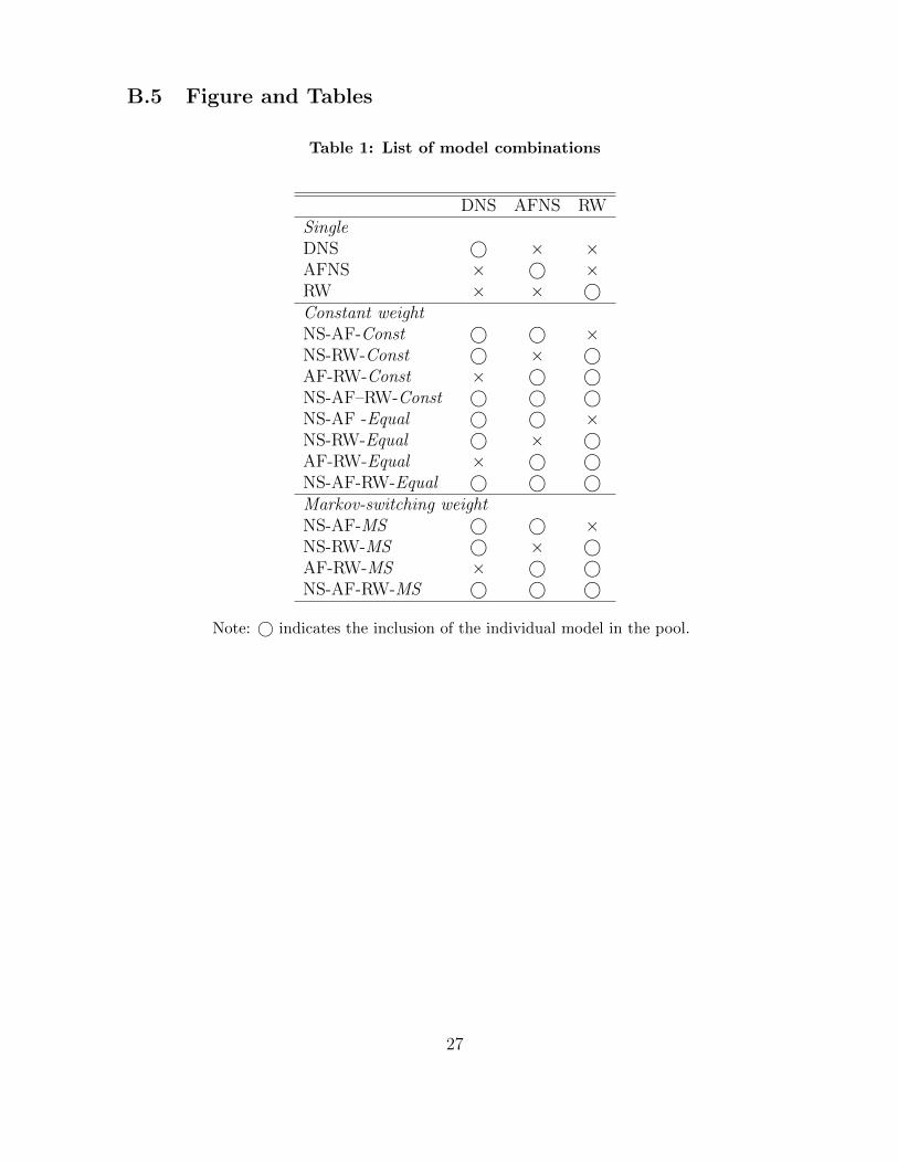
curacy. Table 1 presents 15 competing pooled models with various combinations. We

consider the individual models. Additionally, the linear combinations of two and three

of the alternatives are used for prediction. The model weights can be either constant or

time-varying. For the pooled models with constant weights, the weights are estimated

or equally given. For instance, the NS-AF-RW-Const is the pooled model of the DNS,

AFNS and RW with a constant weight. The NS-AF-RW-MS is the pooled model with

Markov regime-switching weights, in which the model weights vary over time according

to the Markov process. In NS-AF-RW-Equal, each of the model weights is fixed at a

third.

4 Posterior Simulation

This section discusses the posterior sampling scheme for the most general model among

the competing models, the NS-AF-RW-MS model. The others can be estimated as

special cases of the NS-AF-RW-MS model. In the Bayesian context our pooled model

with Markov regime-switching weights is the joint prior distribution of the yield curves

(Y = ytTt=1), the regime indicators (S = stTt=1), the continuous latent variables (X =

xtt=1,2,..,T and F = ftt=1,2,..,T )), and the model parameters (ψ= ΘNS, ΘAF , ΘRW ,

Q, w). Given the joint density, our objective is to simulate the posterior distribution

of (ψ,X,F,S) conditioned on the observed yield curves Y. Its density has the form

π (ψ,X,F,S|Y) ∝ f (Y|ψ,X,F,S)× f (X,F|ψ)× p (S|ψ)× π(ψ) (4.1)

10

where π (ψ) is the prior density of the parameters and p (S|ψ) is the prior density

function for regime-indicators given the parameters; it is specified as the discrete two-

state Markov switching process. f (X,F|S,ψ) is the prior density of the factors and

f (Y|ψ,X,F,S) is the joint conditional density of the observed data.

4.1 Prior

The prior for (ΘNS,ΘAF ) that we give in the paper is set up to reflect the a priori belief

that the yield curve is gently upward sloping and concave on average. Particularly, the

prior of ΘAF should be chosen very carefully because the bond yields are highly nonlinear

to the parameters, and the likelihood surface of the AFNS tends to be irregular. The

irregularity of the posterior surface can be more serious or mitigated depending on the

choice of the prior. We use the prior used in the work of Chib and Kang (2016). As

Chib and Ergashev (2009) suggest, Chib and Kang (2016) arrive at the prior by prior

simulation technique, sampling parameters from the assumed prior, then sampling the

data given the parameters repeating this process many times until the mean of the

resulting prior-implied unconditional distribution of the yield curve is mildly upward

sloping and concave. Chib and Ergashev (2009) and Chib and Kang (2016) document

that this simulation-based prior can smooth out the many local modes of the likelihood

surface.

Additionally, we assume that φ and G are diagonal since this restriction helps im-

prove the predictive accuracy and reduces the computational burden (Christensen et al.

(2011)). Table 2 summarizes our prior.

For regime identification, we impose a restriction that the weight on the DNS model

MNS , denoted by wNS,st , should be higher in regime 2 than in regime 1

0 < wNS,st=1 < wNS,st=2 < 1 and 0 < wNS,st + wAF,,st < 1

where wAF,st is the weight on the AFNS model. For the MS -AF-RW model, the restric-

tion is replaced by

0 < wAF,st=1 < wAF,st=2 < 1.

11

All the restrictions including those of factor identification and regime identification are

imposed through the prior.

4.2 MCMC Sampling

Because the joint posterior distribution in equation (4.1) is not analytically tractable,

we rely on an MCMC simulation method and sample the parameters, factors, regimes,

and predictive yield curves recursively from the joint posterior distribution as follows:

Algorithm 1: MCMC sampling

• Step 1: Sample ΘNS,ΘAF ,ΘRW , w|Y,Q

– Step 1(a): Sample ΘNS,ΘAF ,ΘRW , w|Y,Q

– Step 1(b): Sample Q|Y,S,ΘNS,ΘAF ,ΘRW , w

• Step 2: Sample S|Y,ψ

• Step 3: Sample X|Y,ψ and F|Y,ψ

• Step 4: Sample yT+hHh=1|Y,X,F,S,ψ

More details on MCMC sampling in each step can be found in Appendix B.

5 Predictive Accuracy Measures

We evaluate predictive accuracy using two measures. One is the posterior predictive

criterion (PPC) of Gelfand and Ghosh (1998), which is often used for density forecast

evaluation. The other measure is the root mean squared error (RMSE), which is a

popular measure of point forecast accuracy.3

3Throughout the paper we evaluate the predictive accuracy of multiple individual bond yields insteadof the yield curve in order to see maturity-specific prediction performance of the prediction models andcompare the results with those in the literature. The predictive accuracy of the yield curve can bemeasured by the log predictive likelihood as in Kang (2015).

12

5.0.1 Posterior Predictive Criterion

We follow Zantedeschi et al. (2011) and Chib and Kang (2013) and evaluate the predic-

tive accuracy of the density forecasts by using the posterior predictive criterion (PPC)

of Gelfand and Ghosh (1998). Suppose that yoT+h(τ) is the realized τ -month bond yield,

and E (yT+h(τ)|Y) is the posterior mean of yT+h(τ). Given each pooled model and in-

sample data Y, the PPC for the h-month-ahead posterior predictive density of τ−period

bond yield, PPCY(τ, h) is computed as

PPCY(τ, h) = DY(τ, h) + WY(τ, h)

where

DY(τ, h) = Var (yT+h(τ)|Y)

and

WY(τ, h) =[yoT+h(τ)− E (yT+h(τ)|Y)

]2The term DY(τ, h) is the posterior variance of the predictive yield, which is large when

the model has too many restrictions or redundant parameters. The term WY(τ, h) is the

squared errors and evaluates the predictive goodness-of-fit. Let TH denote the number of

the out-of-sample datasets. Then, the PPC(τ, h) is obtained as the average of PPCY(τ, h)

over the 108(=TH) out-of-samples.

PPC(τ, h) =1

TH

∑Y

PPCY(τ, h)

5.0.2 Root Mean Squared Error

The RMSE of the h-month-ahead bond yield with τ -month to maturity, denoted by

RMSE(τ, h), is given by

RMSE(τ, h) =

√1

TH

∑Y

[yoT+h(τ)− E (yT+h(τ)|Y)

]2.

By definition, smaller values of PPC and RMSE are preferable.

13

6 Empirical Results

In this section, we evaluate and compare the out-of-sample forecasting performance of

the pooled models. We especially concentrate on the predictive gain of pooling the

individual yield curve prediction models.

Our data comprise monthly yields on U.S. government bonds. The time span is from

February 1994 to December 2013. The set of maturities in months is 3, 6, 12, 24, 36, 60,

84, 120. The data are obtained from the Federal Reserve Bank of St. Louis economic

data.

For a model comparison, we calculate PPC and RMSE values from a rolling window

estimation. The window size is 120 months, and the forecast horizon is one through

twelve months. The first out-of-sample period is February 2004 to January 2005, and

the corresponding in-sample period is February 1994 to January 2004. We simulate

the predictive yield curves and compute the squared errors and PPCY. Then, we move

forward the in-sample and out-of-sample by one month and compute the squared errors

and PPCY. This procedure is repeated 108 times where the last out-of-sample period

is January 2013 to December 2013. Finally, we obtain 108 squared errors and PPCYs

for each pair of maturities and forecast horizons. Using these results, we are able to

compute and compare the PPCs and RMSEs of the pooled models with those of the

individual models. The in-sample and out-of-sample pairs are shown in Table 3.

6.1 PPC Comparison

Table 4 presents the best models based on the PPC for each of 96 pairs of maturities

and forecast horizons (12 forecast horizons times eight maturities). For easier reference,

we use shorter model specification indices: “N” stands for the DNS, “A” for the AFNS,

and “R” for the RW. The subscript “E” stands for the equal weights, “C” for the

constant weights, and “M” for the Markov-switching weights. For example, “NRE” in

Table 4 indicates the pooled model of DNS and RW with the equal-weight model (i.e.,

NS-RW-Equal).

Table 4 shows that the best models are pooled models. Particularly, the equal-weight

14

NS-RW model, NS-RW-Equal, outperforms the other models for the maturities of three

months through three years regardless of the forecast horizon. For the seven-year bond

yield, the NS-RW-Equal forecasts best at all the forecast horizons except for the one-

month-ahead forecast. Additionally, pooling all individual models with equal weights is

found to improve the predictive accuracy of five- and ten-year bond yields.

Tables 5 and 6 report the PPCs for the maturities at 1-, 3-, 6-, and 12-month-ahead

horizons to show the relative performance of the alternative models. The PPCs are

normalized by that of the RW model for each maturity. The values larger than one

favor the RW model. Bold entries indicate the best prediction models for each pair of

maturities and forecast horizons.

There are three important implications from the PPC comparison. First, as shown

in Tables 5 and 6, the predictive gain from the pooling method is remarkable. The NS-

RW-Equal consistently outperforms the three individual models across all maturities and

forecast horizons by a substantial margin. Meanwhile, the Bayesian model averaging

tends to pick one of the three individual models. Either the DNS or RW model is

typically selected, but their density forecasting performance is found to be worse than

that of the pooled model of the DNS and RW.

It should be noted that pooling individual models does not guarantee better density

forecasts than selecting one of the individual models. As Tables 5 and 6 demonstrate,

many pooled models produce less accurate forecasts than the DNS or RW model. The

more models included in the pool, the greater the number of parameters that need to be

estimated. Because the information contained in the data is limited and the models in

the pool share the information, prediction can be inefficient, which leads to a very large

posterior variance of the predictive yields.

Second, although the RW model is not the best prediction model for density fore-

casting, all the best model combinations include the RW model in the pool. Therefore,

the RW plays an essential role in improving density forecasting. Third, the theoretical

model, the AFNS, can help produce more accurate density forecasts of long-term bond

yields, and this model should not be excluded from the pool. In particular, for five-year

bond yield prediction, the AFNS is operative at all horizons. This finding is meaningful

15

because the AFNS has been less popular than the DNS and RW models in yield curve

prediction.

It is interesting that the best pooled models have equal model weights. Estimating

the weights, which either are constant or follow the Markov process, can improve in-

sample-fit. At the same time, however, it causes inefficiency. This inefficiency has

already been noted in the literature, for instance by Smith and Wallis (2009), Stock and

Watson (2004), and Winkler and Clemen (1992).

6.2 RMSE Comparison

We move to the point forecasting evaluation of the pooling method. For each pair of

the maturities and forecast horizons, we calculate the RMSE(τ, h) and choose the best

prediction models producing the smallest RMSE value among the competing models.

Table 7 presents the best models for each maturity across forecast horizons. Tables 8 and

9 report the RMSEs for the maturities at 1-, 3-, 6-, and 12-month-ahead horizons to show

the relative prediction ability of the alternative models. Like in the PPC comparison,

the RMSEs are normalized by that of the RW model. Bold entries indicate the best

prediction performance.

Two important findings emerge from the tables. First, in terms of the point predic-

tion, the RW model outperforms the other models in 73 of 96 cases in contrast to the

results from the PPCs. Particularly, the RW produces the most accurate point forecasts

of 3-, 24-, 36-, 60-, and 84-month bond yields at all forecast horizons.

Second, the pooled model, NS-RW-MS forecasts best for six-month bond yields at

long forecast horizons. In addition, the NS-AF-Const is superior in short-term forecast-

ing of the 10-year bond yield. As shown in Tables 8 and 9, however, the differences

between the RMSEs of the two pooled models and the RW model are not substantial.

Therefore, in terms of point forecasts the predictive gain from pooling various yield curve

models does not seem remarkable.

16

6.3 Further Discussion

6.3.1 Forecasting Performance before and after the Crisis

For a robustness check, we split the 108 out-of-sample periods into two subsamples and

evaluate the pooling method based on the PPC and RMSE values. The first and second

54 out-of-sample periods range from January 2004 to June 2008 and from July 2008 to

December 2012, which correspond to the pre-crisis and post-crisis periods, respectively.

Tables 10 and 11 report the best models that achieve the smallest PPC and RMSE

values for the two out-of-sample periods.

As shown in the tables, the best models are different across out-of-sample periods.

Before the crisis the all individual models operate. The AFNS model is especially in-

cluded in most of the best pools, and it performs well even in the point forecasting.

Thus, during the normal period the theoretical model appears reliable. Meanwhile, af-

ter the crisis, the RW seems to be most important as an individual model and for model

combination. The bigger role of the RW model after the crisis can be attributed to the

fact that the RW has an advantage in considering the possibility of a structural change

in the U.S. yield curve dynamics.

On the other hand, the results from the recent 54 out-of-sample forecast periods are

consistent with those from the full forecast periods. This implies that the results from

the recent out-of-sample periods dominate those from the first out-of-sample periods.

6.3.2 Model Weights and Posterior Probability of Regimes

Finally, we discuss the estimates of the model weights using the full sample from February

1994 to December 2013. These estimates can be a measure of the relative importance of

each individual model in the pooled models. Table 12 presents the estimated weights for

the constant-weight model. We find that the DNS model has a higher weight in general,

and the RW model has a lower weight during the full sample period.

However, the model weights do not seem to be constant over time. Table 13 presents

the estimated Markov-switching weights, and Figure 1 plots the posterior probabilities

of regime 2. First, the model weights are strongly regime-dependent, and the regime

changes are drastic over time. As a result, the regimes seem to be well-identified. Recall

17

that the model-specific parameters and model weights are jointly estimated in our work.

For this reason, the parameters in a model are heavily determined by the observations

in the regime when the model has a large weight.

More importantly, the role of the RW model in the pooled models becomes more

important after the recent crisis. For instance, in the case of the NS-AF-RW-MS, the

weights on the DNS and RW models in regime 1 are 0.219 and 0.429, respectively.

Meanwhile, the weights are 0.752 and 0.133 in regime 2. As Figure 1 shows, the posterior

probability of regime 2 has been persistent but decreased drastically around 2008. Hence,

the predictive ability of the DNS model was superior before the recent financial crisis,

but the RW model was dominant after the crisis. As mentioned earlier, this is because

the yield curve dynamics may have undergone a structural change around the crisis

and is detected by the RW process. Table 13 and Figure 1 report the NS-RW-MS and

AF-RW-MS model estimation results and confirm the increasing importance of the RW

model.

One natural question is why dynamic pooling performs worse than static pooling

despite the obvious regime changes in the model weights. This is because the timing of

the regime changes is too close to the end of the sample, and the observations during

regime 1 are not informative enough. As a result, the inefficiency caused by estimating

the transition probabilities and model weights and forecasting the future regimes makes

the dynamic prediction pools perform poorly. For an extended period of time, the pooled

model with the Markov-switching weights may generate more accurate forecasts when

the regime shift is permanent or very persistent. However, if the regime changes are

frequent like in Figure 1 (b), the dynamic pooling approach is not desirable.

7 Conclusion

In this paper we examine whether the pooling method can help improve the accuracy

of yield forecasts. The pool of models includes the dynamic Nelson-Siegel model, the

arbitrage-free Nelson-Siegel model, and the random walk model. We combine these po-

tentially misspecified models in a linear form suggested by Geweke and Amisano (2011),

18

Geweke and Amisano (2012), and Waggoner and Zha (2012). We evaluate the out-of-

sample forecasts of the pooled models based on the PPC and RMSE. The empirical

results of the PPC comparison demonstrate that the pooled model of the DNS and RW

with equal weights produces accurate density forecasts dominating the three individual

models at all maturities and forecast horizons, whereas the predictive gain from the

pooling method does not seem to be substantial in the point forecasts.

The most important implication of our empirical findings is that despite the higher

computational cost, the pooling method is worth trying when multiple bond yield pre-

diction models compete. However, we do not argue that our pooled model is the best

model because another pooled model of different individual models can exhibit better

forecasting performance. The DNS and AFNS models with macroeconomic factors or

regime-switching yield curve models could be included in the pool. In addition, it would

be interesting to examine various approaches to averaging bond yield forecasts and com-

pare their performance as in Clark and McCracken (2010) and De Pooter, Ravazzolo,

and Van Dijk (2010). We leave this as future work.

19

References

Almeida, C. and Vicenteb, J. (2008), “The role of no-arbitrage on forecasting: Lessons

from a parametric term structure model,” Journal of Banking and Finance, 32(12),

2695–2705.

Altavilla, C., Giacomini, R., and Ragusa, G. (2014), “Anchoring the Yield Curve using

Survey Expectations?” European Central Bank Working Paper 1632, 1–28.

Bansal, R. and Zhou, H. (2002), “Term structure of interest rates with regime shifts,”

Journal of Finance, 57(5), 463–473.

Carrieroa, A. and Giacomini, R. (2011), “How useful are no-arbitrage restrictions for

forecasting the term structure of interest rates?” Journal of Econometrics, 164(1),

21–34.

Carter, C. and Kohn, R. (1994), “On Gibbs sampling for state space models,”

Biometrika, 81, 541–53.

Chib, S. (1998), “Estimation and comparison of multiple change-point models,” Journal

of Econometrics, 86, 221–241.

Chib, S. and Ergashev, B. (2009), “Analysis of multi-factor affine yield curve Models,”

Journal of the American Statistical Association, 104, 1324–1337.

Chib, S. and Kang, K. H. (2013), “Change Points in Affine Arbitrage-free Term Structure

Models,” Journal of Financial Econometrics, 11(2), 302–334.

— (2016), “An Efficient Posterior Sampling in Gaussian Affine Term Structure Models,”

Manuscript, 1–28.

Chib, S. and Ramamurthy, S. (2010), “Tailored Randomized-block MCMC Methods

with Application to DSGE Models,” Journal of Econometrics, 155, 19–38.

Christensen, J. H. E., Diebold, F. X., and Rudebusch, G. D. (2011), “The affine

arbitrage-free class of Nelson-Siegel term structure models,” Journal of Economet-

rics, 164, 4–20.

Clark, T. E. and McCracken, M. W. (2010), “Averaging forecasts from VARs with

uncertain instabilities,” Journal of Applied Econometrics, 25(1), 5–29.

20

Dai, Q., Singleton, K. J., and Yang, W. (2007), “Regime shifts in a dynamic term

structure model of U.S. treasury bond yields,” Review of Financial Studies, 20, 1669–

1706.

De Pooter, M. (2007), “Examining the Nelson-Siegel Class of Term Structure Models,”

Tinbergen Institute Discussion Paper.

De Pooter, M., Ravazzolo, F., and Van Dijk, D. J. C. (2010), “Term Structure Fore-

casting Using Macro Factors and Forecast Combination,” FRB International Finance

Discussion Paper No. 993, 1–49.

Del Negro, M., Hasegawa, R. B., and Schorfheide, F. (2016), “Dynamic Prediction

Pools: An Investigation of Financial Frictions and Forecasting Performance,” Journal

of Econometrics, in press.

Diebold, F. X. and Li, C. L. (2006), “Forecasting the term structure of government bond

yields,” Journal of Econometrics, 130, 337–364.

Duffie, G. (2002), “Term premia and interest rate forecasts in affine models,” Journal

of Finance, 57, 405–43.

Duffie, G. and Kan, R. (1996), “A yield-factor model of interest rates,” Mathematical

Finance, 6, 379–406.

Gelfand, A. E. and Ghosh, S. K. (1998), “Model choice: A minimum posterior predictive

loss approach,” Biometrika, 85, 1–11.

Geweke, J. and Amisano, G. (2011), “Optimal prediction pools,” Journal of Economet-

rics, 164(1), 130–141.

— (2012), “Prediction with Misspecified Models,” American Economic Review, 102(3),

482–486.

Kang, K. H. (2015), “Predictive Density Simulation of Yield Curves with a Zero Lower

Bound,” Journal of Empirical Finance, 51–66.

Moench, E. (2008), “Forecasting the yield curve in a data-rich environment: A no-

arbitrage factor-augmented VAR approach,” Journal of Econometrics, 146, 26–43.

Niu, L. and Zeng, G. (2012), “The Discrete-Time Framework of Arbitrage-Free Nelson-

Siegel Class of Term Structure Models,” manuscript, 1–68.

21

Smith, J. and Wallis, K. F. (2009), “A simple explanation of the forecast combination

puzzle*,” Oxford Bulletin of Economics and Statistics, 71, 331–355.

Stock, J. H. and Watson, M. W. (2004), “Combination forecasts of output growth in a

seven-country data set,” Journal of Forecasting, 23, 405–430.

Waggoner, D. and Zha, T. (2012), “Confronting model misspecification in macroeco-

nomics,” Journal of Econometrics, 171(2), 167–184.

Winkler, R. L. and Clemen, R. T. (1992), “Sensitivity of weights in combining forecasts,”

Operations Research, 40, 609–614.

Zantedeschi, D., Damien, P., and Polson, N. G. (2011), “Predictive Macro-Finance

With Dynamic Partition Models,” Journal of the American Statistical Association,

106(494), 427–439.

22

Appendix

A Likelihood

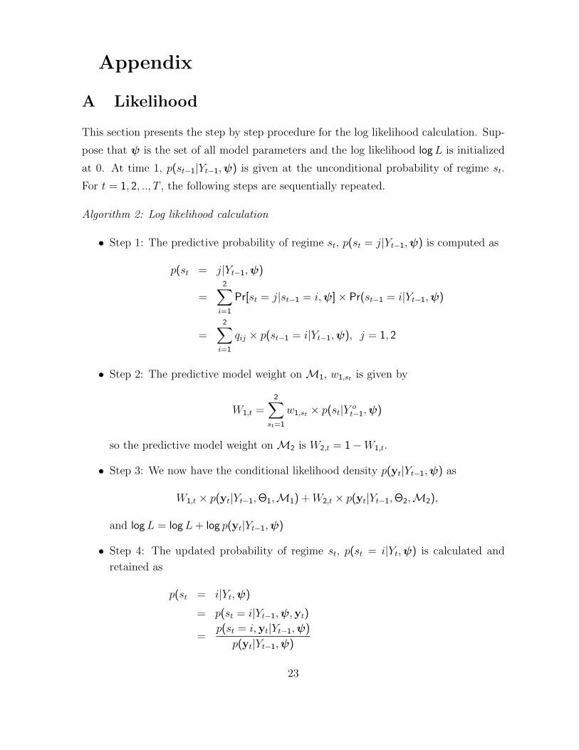
This section presents the step by step procedure for the log likelihood calculation. Sup-

pose that ψ is the set of all model parameters and the log likelihood logL is initialized

at 0. At time 1, p(st−1|Yt−1,ψ) is given at the unconditional probability of regime st.

For t = 1, 2, .., T , the following steps are sequentially repeated.

Algorithm 2: Log likelihood calculation

• Step 1: The predictive probability of regime st, p(st = j|Yt−1,ψ) is computed as

p(st = j|Yt−1,ψ)

=2∑i=1

Pr[st = j|st−1 = i,ψ]× Pr(st−1 = i|Yt−1,ψ)

=2∑i=1

qij × p(st−1 = i|Yt−1,ψ), j = 1, 2

• Step 2: The predictive model weight on M1, w1,st is given by

W1,t =2∑

st=1

w1,st × p(st|Y ot−1,ψ)

so the predictive model weight on M2 is W2,t = 1−W1,t.

• Step 3: We now have the conditional likelihood density p(yt|Yt−1,ψ) as

W1,t × p(yt|Yt−1,Θ1,M1) + W2,t × p(yt|Yt−1,Θ2,M2),

and logL = logL + log p(yt|Yt−1,ψ)

• Step 4: The updated probability of regime st, p(st = i|Yt,ψ) is calculated and

retained as

p(st = i|Yt,ψ)

= p(st = i|Yt−1,ψ,yt)

=p(st = i,yt|Yt−1,ψ)

p(yt|Yt−1,ψ)

23

=p(yt|Yt−1,ψ, st = i)p(st = i|Yt−1,ψ)

p(yt|Yt−1,ψ)for i = 1, 2

where the predictive density of yt given st is simply given by

p(yt|Yt−1,ψ, st)= w1,st × p(yt|Yt−1,Θ1,M1) + (1− w1,st)× p(yt|Yt−1,Θ2,M2)

• Step 5: t = t + 1 and go to Step 1 if t ≤ T

B Details of MCMC Sampling

We now discuss the details of each MCMC step. The burn-in is 1,000 and the MCMC

simulation size beyond the burn-in is 10,000.

B.1 Parameters Sampling

First, Θ = (ΘNS,ΘAF ,ΘRW , w) are simulated by the tailored randomized blocking

Metropolis-Hastings algorithm (TaRB-MH, Chib and Ramamurthy (2010)). We note

that the posterior density of Θ is proportional to the product of the likelihood and the

prior because

π (Θ|Y,Q) ∝ f (Y|ψ)× π(Θ). (B.1)

We simulate Θ|Y,Q rather than Θ|Y,S,X,Q by integrating out the regimes and latent

factors because the former is more efficient than the latter. The likelihood computation

is illustrated in Appendix A.

In every MCMC iteration, we apply the TaRB-MH method and sample Θ given

(Y,Q). This algorithm is particularly useful when the posterior density is high-dimensional

and its surface is possibly irregular. For the technical details, refer to Chib and Rama-

murthy (2010) or Chib and Kang (2013).

Next, because the transition probability Q is independent of (Y,Θ) given the regimes

S, it is sampled from

Q|S.

Moreover, its prior is conjugate, and the transition probabilities are sampled from a beta

distribution.

B.2 Regime Sampling

The time-series of the regimes S is simulated in one block by the multi-move method

(Chib (1998)). This method consists of two stages. The first stage is to calculate the

24

filtered probabilities, Pr(st|Yt,ψ) as

Pr(st = j|Yt,ψ) =

∑2i=1 p(yt|Yt−1, st = j,ψ)× Pr(st = j|st−1 = i,ψ)∑2

j=1

[∑2i=1 p(yt|Yt−1, st = j,ψ)× Pr(st = j|st−1 = i,ψ)

]=

∑2i=1 p(yt|Yt−1, st = j,ψ)× qij∑2

j=1

[∑2i=1 p(yt|Yt−1, st = j,ψ)× qij

]for j = 1, 2. Then, the conditional density of yt p(yt|Yt−1, st,ψ) is computed as the linear

combination of the model-specific conditional densities of yt: p(yt|Yt−1,ΘNS,MNS),

p(yt|Yt−1,ΘAF ,MAF ), and p(yt|Yt−1,ΘRW ,MRW ). That is,

p(yt|Yt−1, st,ψ)

= wNS,st × p(yt|Yt−1,ΘNS,MNS) + wAF,st × p(yt|Yt−1,ΘAF ,MAF )

+(1− wNS,st − wAF,st)× p(yt|Yt−1,ΘRW ,MRW )

These model-specific conditional densities are already given in equations (3.5), (3.14),

and (3.16).

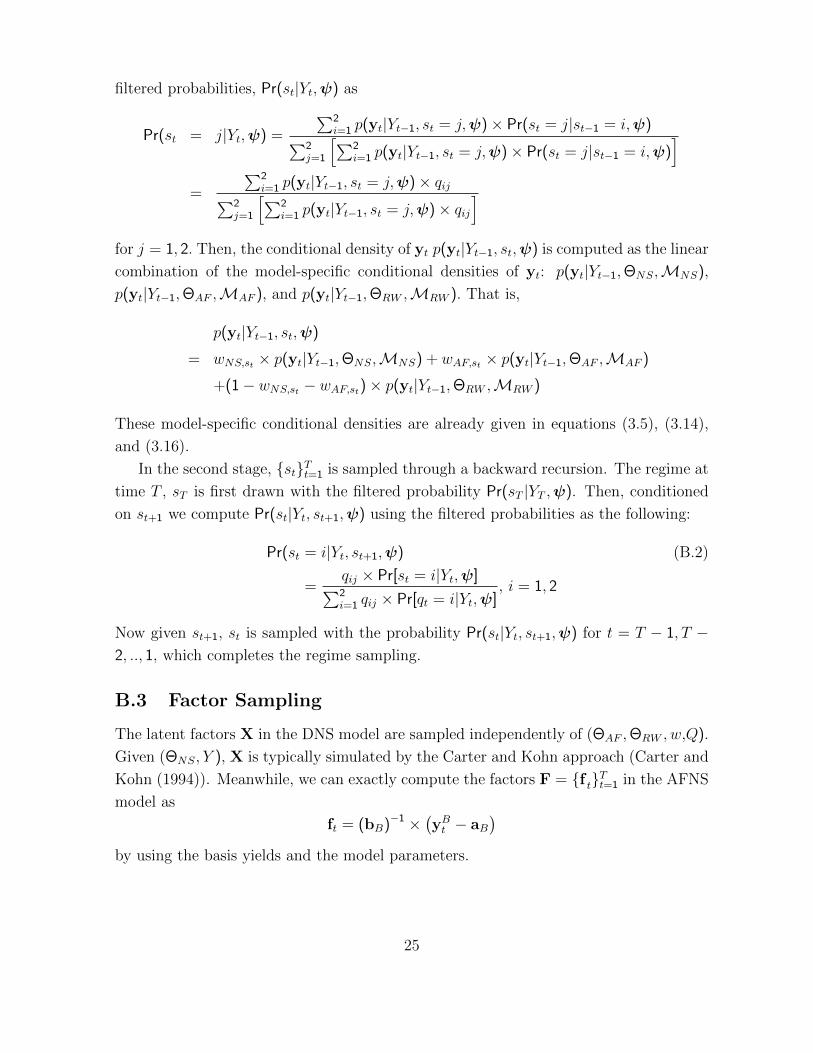
In the second stage, stTt=1 is sampled through a backward recursion. The regime at

time T , sT is first drawn with the filtered probability Pr(sT |YT ,ψ). Then, conditioned

on st+1 we compute Pr(st|Yt, st+1,ψ) using the filtered probabilities as the following:

Pr(st = i|Yt, st+1,ψ) (B.2)

=qij × Pr[st = i|Yt,ψ]∑2i=1 qij × Pr[qt = i|Yt,ψ]

, i = 1, 2

Now given st+1, st is sampled with the probability Pr(st|Yt, st+1,ψ) for t = T − 1, T −2, .., 1, which completes the regime sampling.

B.3 Factor Sampling

The latent factors X in the DNS model are sampled independently of (ΘAF ,ΘRW , w,Q).

Given (ΘNS, Y ), X is typically simulated by the Carter and Kohn approach (Carter and

Kohn (1994)). Meanwhile, we can exactly compute the factors F = f tTt=1 in the AFNS

model as

ft = (bB)−1 ×(yBt − aB

)by using the basis yields and the model parameters.

25

B.4 Predictive Yield Curve Sampling

Each MCMC cycle is completed by sampling the posterior predictive draws given (Y,

X, F, S, ψ). For each posterior draw (yT ,xT , fT , sT ,ψ) and forecast horizon of h =

1, 2, .., H, we first simulate the predictive draws of the factors xT+h, fT+hHh=1. Given the

factors and parameters, the model-specific predictive bond yields are generated within

the individual model specifications. Next, the predictive regime sT+hHh=1 is sampled

by the Markov-switching process, and it determines the model weights for each forecast

horizon. Finally, the predictive yield curve is computed as the linear combination of the

model-specific predictive yield curves and is retained as the posterior predictive draws.

The following algorithm summarizes the predictive yield curve simulation.

Algorithm 3: Posterior predictive distribution simulation

• Step 1: Sample the factors xT+hHh=1|X,ΘNS and fT+hHh=1|F,ΘAF

• Step 2: Sample the model-specific predictive yields

yNS,T+hHh=1|X,ΘNS, yAF,T+hHh=1|F,ΘAF , and yRW,T+hHh=1|Y,ΘRW

• Step 3: Sample the predictive regimes, sT+hHh=1|S,Q

• Step 4: For h = 1, 2, .., H, compute the predictive yield curve as

yT+h = wNS,sT+h× yNS,T+h + wAF,sT+h

× yAF,T+h

+(1− wNS,sT+h− wAF,sT+h

)× yRW,T+h

• Step 5: Retain yT+hHh=1 as a posterior predictive draw

26

B.5 Figure and Tables

Table 1: List of model combinations

DNS AFNS RWSingleDNS © × ×AFNS × © ×RW × × ©Constant weightNS-AF-Const © © ×NS-RW-Const © × ©AF-RW-Const × © ©NS-AF–RW-Const © © ©NS-AF -Equal © © ×NS-RW-Equal © × ©AF-RW-Equal × © ©NS-AF-RW-Equal © © ©Markov-switching weightNS-AF-MS © © ×NS-RW-MS © × ©AF-RW-MS × © ©NS-AF-RW-MS © © ©

Note: © indicates the inclusion of the individual model in the pool.

27

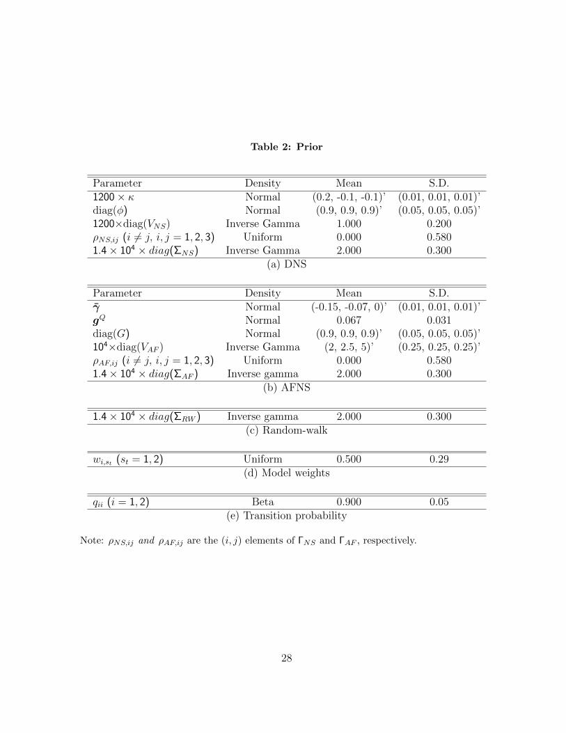
Table 2: Prior

Parameter Density Mean S.D.1200× κ Normal (0.2, -0.1, -0.1)’ (0.01, 0.01, 0.01)’diag(φ) Normal (0.9, 0.9, 0.9)’ (0.05, 0.05, 0.05)’1200×diag(VNS) Inverse Gamma 1.000 0.200ρNS,ij (i 6= j, i, j = 1, 2, 3) Uniform 0.000 0.5801.4× 104 × diag(ΣNS) Inverse Gamma 2.000 0.300

(a) DNS

Parameter Density Mean S.D.γ Normal (-0.15, -0.07, 0)’ (0.01, 0.01, 0.01)’gQ Normal 0.067 0.031diag(G) Normal (0.9, 0.9, 0.9)’ (0.05, 0.05, 0.05)’104×diag(VAF ) Inverse Gamma (2, 2.5, 5)’ (0.25, 0.25, 0.25)’ρAF,ij (i 6= j, i, j = 1, 2, 3) Uniform 0.000 0.5801.4× 104 × diag(ΣAF ) Inverse gamma 2.000 0.300

(b) AFNS

1.4× 104 × diag(ΣRW ) Inverse gamma 2.000 0.300(c) Random-walk

wi,st (st = 1, 2) Uniform 0.500 0.29(d) Model weights

qii (i = 1, 2) Beta 0.900 0.05(e) Transition probability

Note: ρNS,ij and ρAF,ij are the (i, j) elements of ΓNS and ΓAF , respectively.

28

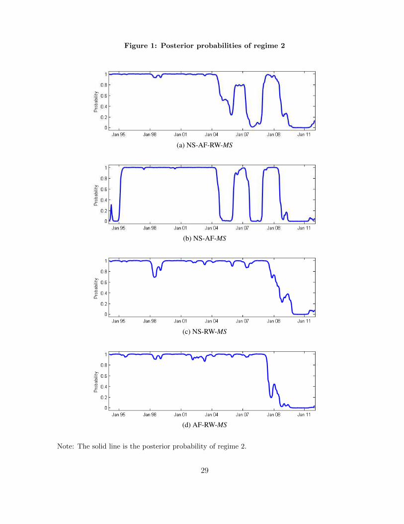
Figure 1: Posterior probabilities of regime 2

(a) NS-AF-RW-MS

(b) NS-AF-MS

(c) NS-RW-MS

(d) AF-RW-MS

Note: The solid line is the posterior probability of regime 2.

29

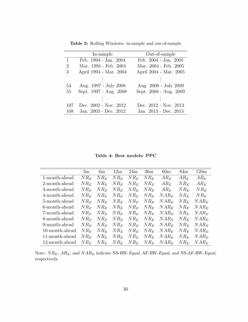
Table 3: Rolling Windows: in-sample and out-of-sample

In-sample Out-of-sample1 Feb. 1994 - Jan. 2004 Feb. 2004 - Jan. 20052 Mar. 1994 - Feb. 2004 Mar. 2004 - Feb. 20053 April 1994 - Mar. 2004 April 2004 - Mar. 2005

......

54 Aug. 1997 - July 2008 Aug. 2008 - July 200955 Sept. 1997 - Aug. 2008 Sept. 2008 - Aug. 2009

......

107 Dec. 2002 - Nov. 2012 Dec. 2012 - Nov. 2013108 Jan. 2003 - Dec. 2012 Jan. 2013 - Dec. 2013

Table 4: Best models: PPC

3m 6m 12m 24m 36m 60m 84m 120m1-month-ahead NRE NRE NRE NRE NRE ARE ARE ARE

2-month-ahead NRE NRE NRE NRE NRE ARE NRE ARE

3-month-ahead NRE NRE NRE NRE NRE ARE NRE NRE

4-month-ahead NRE NRE NRE NRE NRE NARE NRE NRE

5-month-ahead NRE NRE NRE NRE NRE NARE NRE NARE








Note: NRE , ARE , and NARE indicate NS-RW-Equal, AF-RW-Equal, and NS-AF-RW-Equal,

respectively.

30

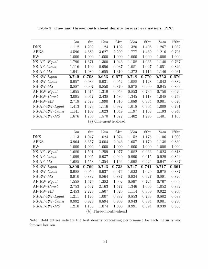
Table 5: One- and three-month ahead density forecast evaluations: PPC

3m 6m 12m 24m 36m 60m 84m 120mDNS 1.112 1.209 1.124 1.102 1.320 1.408 1.267 1.032AFNS 4.596 4.583 3.627 2.200 1.777 1.469 1.216 0.795RW 1.000 1.000 1.000 1.000 1.000 1.000 1.000 1.000NS-AF -Equal 1.790 1.671 1.300 1.043 1.158 1.035 1.140 0.767NS-AF-Const 1.116 1.102 0.956 0.937 1.081 1.027 1.051 0.846NS-AF-MS 1.941 1.980 1.655 1.310 1.272 1.116 1.146 0.931NS-RW-Equal 0.749 0.708 0.653 0.677 0.748 0.779 0.752 0.676NS-RW-Const 0.957 0.983 0.931 0.952 1.088 1.128 1.042 0.882NS-RW-MS 0.887 0.907 0.850 0.870 0.978 0.999 0.945 0.833AF-RW-Equal 1.655 1.615 1.319 0.953 0.853 0.736 0.750 0.620AF-RW-Const 3.095 3.047 2.438 1.586 1.345 1.118 1.048 0.749AF-RW-MS 2.719 2.578 1.990 1.310 1.089 0.934 0.901 0.670NS-AF-RW-Equal 1.413 1.329 1.116 0.982 1.018 0.904 1.009 0.791NS-AF-RW-Const 1.141 1.109 1.023 1.049 1.197 1.168 1.193 0.940NS-AF-RW-MS 1.676 1.730 1.570 1.372 1.402 1.296 1.401 1.163

(a) One-month-ahead


(b) Three-month-ahead

Note: Bold entries indicate the best density forecasting performance for each maturity and

forecast horizon.

31

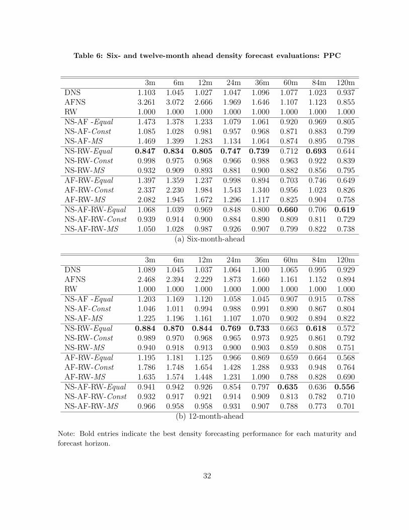
Table 6: Six- and twelve-month ahead density forecast evaluations: PPC


(a) Six-month-ahead


(b) 12-month-ahead

Note: Bold entries indicate the best density forecasting performance for each maturity and

forecast horizon.

32

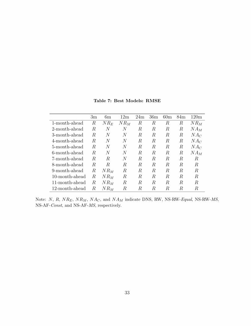
Table 7: Best Models: RMSE

3m 6m 12m 24m 36m 60m 84m 120m1-month-ahead R NRE NRM R R R R NRM

2-month-ahead R N N R R R R NAM3-month-ahead R N N R R R R NAC4-month-ahead R N N R R R R NAC5-month-ahead R N N R R R R NAC6-month-ahead R N N R R R R NAM7-month-ahead R R N R R R R R8-month-ahead R R R R R R R R9-month-ahead R NRM R R R R R R10-month-ahead R NRM R R R R R R11-month-ahead R NRM R R R R R R12-month-ahead R NRM R R R R R R

Note: N , R, NRE , NRM , NAC , and NAM indicate DNS, RW, NS-RW-Equal, NS-RW-MS,

NS-AF-Const, and NS-AF-MS, respectively.

33

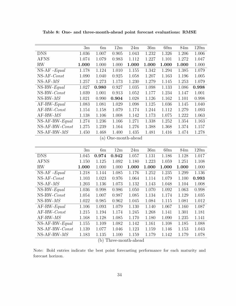
Table 8: One- and three-month-ahead point forecast evaluations: RMSE


(a) One-month-ahead


(b) Three-month-ahead

Note: Bold entries indicate the best point forecasting performance for each maturity and

forecast horizon.

34

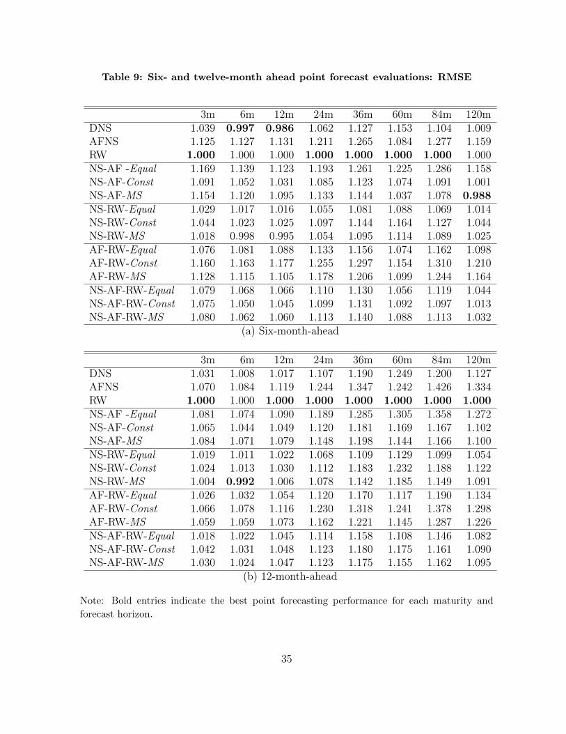
Table 9: Six- and twelve-month ahead point forecast evaluations: RMSE


(a) Six-month-ahead


(b) 12-month-ahead

Note: Bold entries indicate the best point forecasting performance for each maturity and

forecast horizon.

35

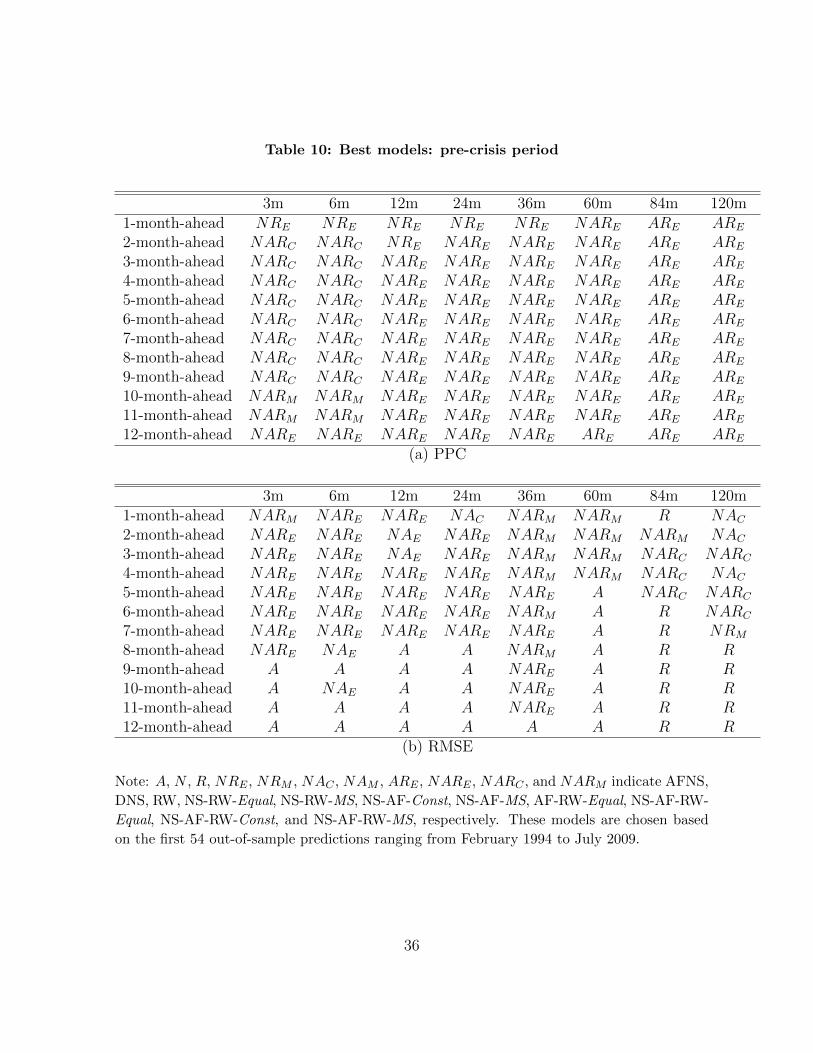
Table 10: Best models: pre-crisis period

3m 6m 12m 24m 36m 60m 84m 120m1-month-ahead NRE NRE NRE NRE NRE NARE ARE ARE

2-month-ahead NARC NARC NRE NARE NARE NARE ARE ARE

3-month-ahead NARC NARC NARE NARE NARE NARE ARE ARE







10-month-ahead NARM NARM NARE NARE NARE NARE ARE ARE

11-month-ahead NARM NARM NARE NARE NARE NARE ARE ARE

12-month-ahead NARE NARE NARE NARE NARE ARE ARE ARE

(a) PPC

3m 6m 12m 24m 36m 60m 84m 120m1-month-ahead NARM NARE NARE NAC NARM NARM R NAC2-month-ahead NARE NARE NAE NARE NARM NARM NARM NAC3-month-ahead NARE NARE NAE NARE NARM NARM NARC NARC

4-month-ahead NARE NARE NARE NARE NARM NARM NARC NAC5-month-ahead NARE NARE NARE NARE NARE A NARC NARC

6-month-ahead NARE NARE NARE NARE NARM A R NARC

7-month-ahead NARE NARE NARE NARE NARE A R NRM

8-month-ahead NARE NAE A A NARM A R R9-month-ahead A A A A NARE A R R10-month-ahead A NAE A A NARE A R R11-month-ahead A A A A NARE A R R12-month-ahead A A A A A A R R

(b) RMSE

Note: A, N , R, NRE , NRM , NAC , NAM , ARE , NARE , NARC , and NARM indicate AFNS,

DNS, RW, NS-RW-Equal, NS-RW-MS, NS-AF-Const, NS-AF-MS, AF-RW-Equal, NS-AF-RW-

Equal, NS-AF-RW-Const, and NS-AF-RW-MS, respectively. These models are chosen based

on the first 54 out-of-sample predictions ranging from February 1994 to July 2009.

36

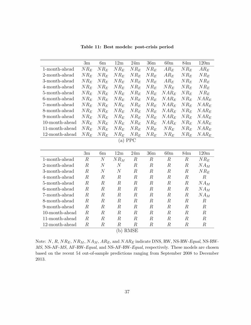
Table 11: Best models: post-crisis period

3m 6m 12m 24m 36m 60m 84m 120m1-month-ahead NRE NRE NRE NRE NRE ARE NRE ARE



4-month-ahead NRE NRE NRE NRE NRE NRE NRE NRE

5-month-ahead NRE NRE NRE NRE NRE NARE NRE NRE






11-month-ahead NRE NRE NRE NRE NRE NRE NRE NARE

12-month-ahead NRE NRE NRE NRE NRE NRE NRE NARE

(a) PPC

3m 6m 12m 24m 36m 60m 84m 120m1-month-ahead R N NRM R R R R NRE

2-month-ahead R N N R R R R NAM3-month-ahead R N N R R R R NRE

4-month-ahead R R R R R R R R5-month-ahead R R R R R R R NAM6-month-ahead R R R R R R R NAM7-month-ahead R R R R R R R NAM8-month-ahead R R R R R R R R9-month-ahead R R R R R R R R10-month-ahead R R R R R R R R11-month-ahead R R R R R R R R12-month-ahead R R R R R R R R

(b) RMSE

Note: N , R, NRE , NRM , NAM , ARE , andNARE indicate DNS, RW, NS-RW-Equal, NS-RW-

MS, NS-AF-MS, AF-RW-Equal, and NS-AF-RW-Equal, respectively. These models are chosen

based on the recent 54 out-of-sample predictions ranging from September 2008 to December

2013.

37

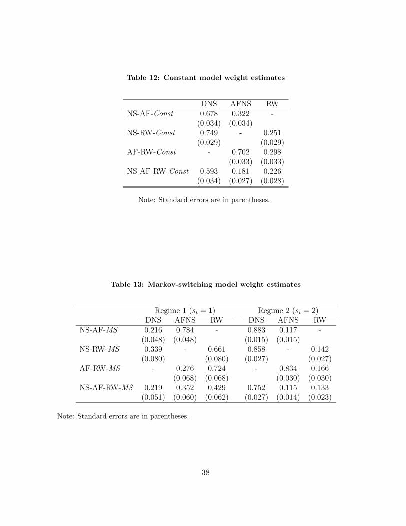
Table 12: Constant model weight estimates

DNS AFNS RWNS-AF-Const 0.678 0.322 -

(0.034) (0.034)NS-RW-Const 0.749 - 0.251

(0.029) (0.029)AF-RW-Const - 0.702 0.298

(0.033) (0.033)NS-AF-RW-Const 0.593 0.181 0.226

(0.034) (0.027) (0.028)

Note: Standard errors are in parentheses.

Table 13: Markov-switching model weight estimates

Regime 1 (st = 1) Regime 2 (st = 2)DNS AFNS RW DNS AFNS RW

NS-AF-MS 0.216 0.784 - 0.883 0.117 -(0.048) (0.048) (0.015) (0.015)

NS-RW-MS 0.339 - 0.661 0.858 - 0.142(0.080) (0.080) (0.027) (0.027)

AF-RW-MS - 0.276 0.724 - 0.834 0.166(0.068) (0.068) (0.030) (0.030)

NS-AF-RW-MS 0.219 0.352 0.429 0.752 0.115 0.133(0.051) (0.060) (0.062) (0.027) (0.014) (0.023)

Note: Standard errors are in parentheses.

38

forecasting the term structure of interest rates with potentially … · 2016-11-21 · forecasting...

Documents