1

Forecasting technology costs via the Learning Curve – Myth or Magic?

Stephan Alberth*

Forward – by Yuri Ermoliev†

The concept of learning curves (experience curves) was first introduced by Wright (1936). By way of empirical evidence he found that unit costs for different inputs when compared to the cumulative production of airplanes exponentially declines with the cumulative level of production as a result of “learning-by-doing”. This relates heavily to so-called increasing returns, non-convexities and the path dependence of technological developments with potential “lock-in” states. As a result, purely market mechanisms fail to select new “expensive” technologies which may become “cheap” and environmentally sound under proper early investments. The learning curve, in fact, shows the investment necessary to make the new technology competitive with cheap mature technologies, but it does not predict when the break-even point occurs. The time of break-even depends on policy variables affecting deployment rates of new technologies and various uncertainties affecting their learning curves restricting straight forward extrapolations of declining costs. Since learning curves represent combined effects of a large number of factors (see D.L. Bodde, Technological Review, March/April 1976), they cannot be used reliably for short-term decisions. As IIASA‟s studies show (Gritsevski, Nakicenovic, 2000), the use of learning curves plays a decisive role for comparative analysis of long-term competitive technologies, in particular low-cost paths to CO² stabilization. A key issue in this analysis is proper treatment of involved uncertainties. Unfortunately, there are only a few publications attempting to systematically analyse uncertainties affecting learning curves. In general it may require a rather delicate approach that is able to deal with potential outliers, “hard” historical observations and “staff” data from expert‟s opinions and scenarios. The main goal of this paper is to fill a gap in this important research area.

* PhD candidate, Judge Business School, University of Cambridge.

† Institute Scholar, Integrated Modeling Environment Project

2

Abstract

To further our understanding of the effectiveness of learning or experience curves to forecast technology costs, a statistical analysis using historical data has been carried out. Three hypotheses have been tested using available data sets that together shed light on the ability of experience curves to forecast future technology costs. The results indicate that the Single Factor Learning Curve is a highly effective estimator of future costs with little bias when errors were viewed in their log format. However it was also found that due to the convexity of the log curve an overestimation of potential cost reductions arises when returned tothe results were considered in their monetary units. Furthermore the effectiveness of increasing weights for more recent data was tested using Weighted Least Squares with exponentially increasing weights. This resulted in forecasts that were typically less biased than when using Ordinary Least Square and highlighted the potential benefits of this method.

3

Acknowledgements

This paper is based on research carried out at IIASA under the supervision of Yuri Ermoliev as part of the YSSP research program.

I would like to thank Chris Hope, Arnulf Grübler, Leo Schrattenholzer, Marek Makowski, Nebojsa Nakicenovic, Clas Otto Wene, David Victor, Brian O‟Neil, Marvin Lieberman, Oswoldo Lucon, Paul Maycock, Ulrika Colpier Cleason and Nadejda Victor for their contributions with data, ideas or words of caution during this research project.

I am also very grateful for the support of the Cambridge University Energy Policy Research Group (EPRG).

4

1. Introduction

In order to improve our understanding of the effectiveness of learning curves or experience curves for forecasting technology costs, a statistical analysis of a range of technologies has been carried out. Three hypotheses have been tested using available data sets that together shed light on the ability for learning curves to forecast future technology costs. The aims of this research are similar to that of McDonald and Schrattenholzer (2001, p255) who analysed the variability and evaluated the usefulness of learning curves for applications in long-term energy models. However, where they focused on the variability of the actual long term learning rates between energy technologies, this research directly evaluates the ability for the Single Factor Learning Curve (SFLC) to make forecasts about future costs using historical data. Throughout the text reference has been made to both learning curves and experience curves. The term „learning curve‟ has been used to refer to the general concept while the term “experience curve” refers more specifically to the calculation of costs (or prices) as a function of cumulative experience.

Initially the hypothesis that experience curves can be used as an unbiased estimator of future costs has been tested by calculating the distribution of forecast errors when using historical experience curve rates as a predictor. The second hypothesis tested refers to the question „do experience curves as a predictor of future costs improve as more experience is accumulated?‟ This has been tested by way of an empirical analysis comparing the forecasts made with fewer data points to forecasts that were made later on with access to a greater number of data points. Finally the hypothesis has been tested relating to whether the explaining power of older data is less important than that of the more recent data by using weighted least squares with exponentially higher weights being placed on more recent data. Together the results of this research provides an initial appraisal of the usefulness of experience curves for forecasting as well as some interesting data in terms of variability of forecasting errors both for the individual technologies tested as well as the set of forecasts aggregated over all technologies.

In the absence of easy to use and reliable models or methods to make cost projections for new technologies, experience curves have been used extensively in the literature to provide indications of “potential” cost reduction as experience is gained and “potential” learning investments required to reach a situation of break-even, the point where a new technology surpasses an incumbent technology in terms of cost-effectiveness. The method has nevertheless been criticised for a number of its inherent weaknesses. First it is important to note that learning curves are a heuristic measure without a solid

5

theoretical basis although further work continues in this area (such as by Wene author of IEA 2000). The simplicity of the SFLC that calculated cost/price uniquely as a function of cumulative experience, can also be seen as a weakness since, for instance, it does not take into account R&D or other technology specific factors. On the other hand the 2 Factor Learning Curve (2FLC), usually incorporating cumulative production and cumulative R&D spending, is difficult to implement due to its need for hard to acquire data and also, in the case for wind and solar at least, because it has shown poor results (Papineau 2004). Studies based on multi-factor learning curves use technical factors to explain changes in the dependant variable (usually price or cost) and have been shown to offer highly informative results, such as in the case of the flying fortress (Mishina 1999), the chemical industry (Lieberman 1984) and wind power (Coulomb & Neuhoff 2005) . Nevertheless, despite their evident relevance in describing historical trends, when it comes to predicting future costs one faces a problem of compounding uncertainties. That is, not only should the relationship between independent and dependant variables be maintained but one must also be able to forecast future values for what are generally highly uncertain independent variables.

A further perceived limitation is the absence of floor costs that have been shown to exist particularly for technologies that reach maturity. One explanation is that when growth of experience begins to decline, „forgetting by not doing‟ becomes an important factor. On the other hand, most technologies relevant to climate change are still far from reaching maturity. One fortuitous result is that learning curves used in this field may be somewhat more accurate than learning curves used to describe cost reductions in more mature technologies. To take advantage of this situation focus has remained during the project on technologies that continued to grow. Another possible limitation is that improvements in quality, such as in the automotive industry, can offset the expected reductions in cost (examples given in McDonald & Schrattenholzer 2001and Colpier & Cornland 2002). Coulomb & Neuhoff (2005) suggest that in the case of wind power, turbine size could also have an important effect on learning rates and that wind turbines have suffered from recent diseconomies of scale, at least on the production side. Once they converge to an optimal size, one could expect “faster cost reductions” since simple cost reductions would then be the main focus. Such examples of structural change can lead to a dynamically shifting learning rate, something that exponentially increasing weights given to more recent data points would help to rectify.

To better understand the usefulness and robustness of the experience curve paradigm, this paper measures the effectiveness a posteriori of the simple SFLC to forecast future costs for a range of technologies. A number of different methods to calculate the experience curve parameters are compared including Ordinary Least Squares (OLS), the standard method used for experience curve calculations and Weighted Least Squares (WLS) with exponentially higher weightings going to more recent information. This assumes that the most recent data offers a better representation of how a technology will continue to learn than older data. The Robust Least Squares (RLS) method, that weights the data according to the deviation from the line of best fit, was also utilised with the aim

6

of reducing the effect of outliers. This puts less weight on sudden changes in market conditions or various sources of data error that could cause strong temporary fluctuations in price.

In all, the fundamental concept of this research paper is similar to that of Everett and Farghal (1994, 1997a and 1997b) in their use of learning curves to predict total time or cost required for future cycles of a repetitive construction activity. The emphasis and methods used, however, are quite different. In particular their work focussed on an area that should in theory be far easier to forecast since the projects were generally over a shorter time period, remained more or less identical and did not cross regional boundaries. Furthermore they focused on the use of smoothing techniques that reduced the importance of the more recent data and looked at the error of total costs required to reach the „final‟ cumulative output. Since in this paper we are dealing with technologies that are changing over 10 or 20 years or longer with a greater likelihood of fundamental shifts in the learning curve, we have considered weighing data in such a way that recent data has a stronger influence over forecasts. Furthermore, since there is generally no pre-decided limit to the total output of a technology, this paper also makes forecasts for a set number of doublings of cumulative capacity with special effort to capture the uncertainty distributions of the forecasts made. Despite the strong grounding of this paper in actual historical statistics there still remains scope for sample selection bias since all of the technologies selected have certainly reached some level of success. Nevertheless by evaluating the effectiveness of the learning curve and measuring the uncertainties surrounding its forecasts, the paper is able to respond in part to the acknowledged limitations of the experience curve model. Such limitations include comments by Wene (IEA 2000) where he highlighted “the risk that expected benefits will not materialise,” and of Grübler et al. (1998 p510) who warned of the dangers of “„best guess‟ parameterisation”.

The following section provides a literature review of learning curves and their ability to predict future learning investments. The forecast model is then discussed as are the assumptions made and the data sources used. This is followed by the results of the model and a discussion on the ability for technology learning investments to be predicted through learning curve methods.

2. Literature review of learning curves

In the overview of the 1998 Energy Economics special issue on „The Optimal Timing of Climate Abatement‟, Carraro and Hourcade pointed out the notable influence that learning appeared to have on the calculation of abatement costs. According to their survey of Energy-Economics-Environment (E3) models, learning introduced around a 50% drop in abatements costs. The IEA publication „Experience Curves for Energy Technology Policy‟ (IEA 2000) presents a broad overview of the work covered up to the end of the 1990‟s and also presents the findings from the 1999 IEA workshop on this subject. Their recommendation was that experience effects should be “explicitly considered in

7

exploring scenarios to reduce CO2 emissions and calculating the cost of reaching emissions targets” (IEA 2000, p114).

Empirical evidence for learning curves was first discovered in 1925 at the Wright-Patterson Air Force Base where it was discovered found that plotting an aeroplane‟s manufacturing input against cumulative number of planes built on a log-log scale produced a linear result as presnted. The benefits in efficiency found were proclaimed by Wright as being the result of “Learning by Doing” in his 1936 publication. This “learning curve” was calculated for a manufacturing input such as time as shown in Equation (1), where Nt was the labour requirements per unit output for period (t), Xt the cumulative output in units by the end of the period. In the equation „a‟ is the constant and „b‟ the learning coefficient as determined by regression analysis:

tt XbaN loglog (1)

The next major advancement in learning curves was made by Arrow in his 1962 publication (Arrow 1962, IEA 2000). He generalised the learning concept and put forward the idea that technical learning was a result of experience gained through engaging in the activity itself. Undertaking an activity, Arrow suggested, leads to a situation where “favourable responses are selected over time” (Arrow 1962, p156).

During the 1960‟s the Boston Consulting Group (BCG) popularised the learning curve. They further developed the theory and published a number of articles on the subject (BCG 1968 in IEA 2000, Henderson 1973a, Henderson 1973b). They also coined the term “experience curve”, as distinct from “learning curve” which related to „unit total costs‟ as a function of „cumulative output‟, rather than „unit inputs‟ as a function of „cumulative output‟ as shown in Equation (2). In this equation the cost per unit „Ct‟ depends on the cumulative number of units produced „Xt‟ and the constant „a‟ and coefficient „b‟ that that can be found using regression analysis. This can be rewritten into a simpler form, as shown by Equations (3) to Equation (4). The Progress Ratio (PR) defined in Equation (5) and Equation (6) is a widely used ratio of final to initial costs associated with a doubling of cumulative output. The Learning Rate (LR) represents the proportional cost savings made for a doubling of cumulative output as presented in Equation (7).

tt XbaC loglog (2)

b

t XconstC (3)

b

t

tX

XCC

0

0

(4)

The so called Progress Ratio (PR) and the Learning Rate (LR) are defined as follows:

,2

0

0

0

b

t

X

X

C

CPR (5)

8

,2 bPR (6)

PRLR 1 . (7)

Despite a strong preference for the use of cost data for this type of analysis, lack of such information often leads to replacing cost with price data which is more readily available (IEA 2000). This leads to an equivalent formulation as presented in Equation (8) and Equation (9).

tt XbaP loglog, (8)

b

t

tX

XPP

0

0

, (9)

Where b is the learning coefficient and P0 and X0 are the price and cumulative output during the initial period.

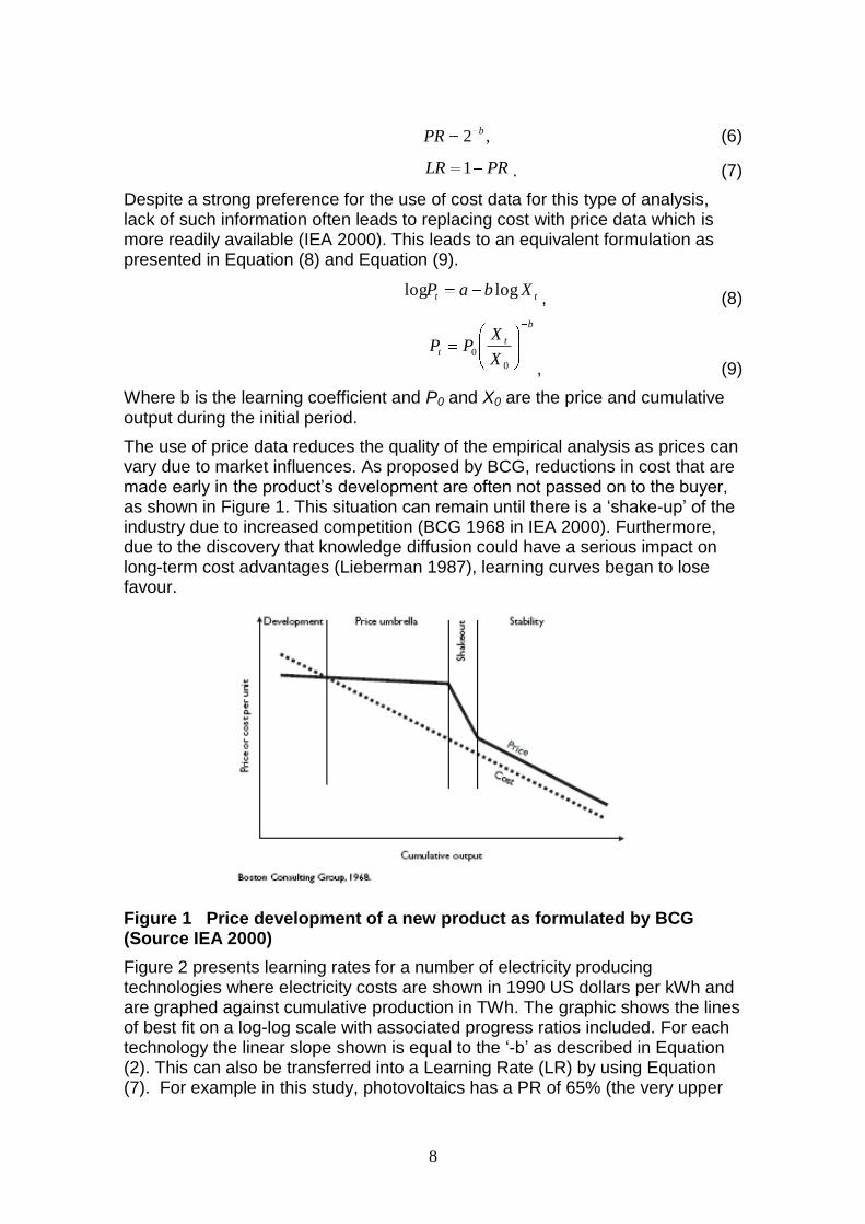
The use of price data reduces the quality of the empirical analysis as prices can vary due to market influences. As proposed by BCG, reductions in cost that are made early in the product‟s development are often not passed on to the buyer, as shown in Figure 1. This situation can remain until there is a „shake-up‟ of the industry due to increased competition (BCG 1968 in IEA 2000). Furthermore, due to the discovery that knowledge diffusion could have a serious impact on long-term cost advantages (Lieberman 1987), learning curves began to lose favour.

Figure 1 Price development of a new product as formulated by BCG (Source IEA 2000)

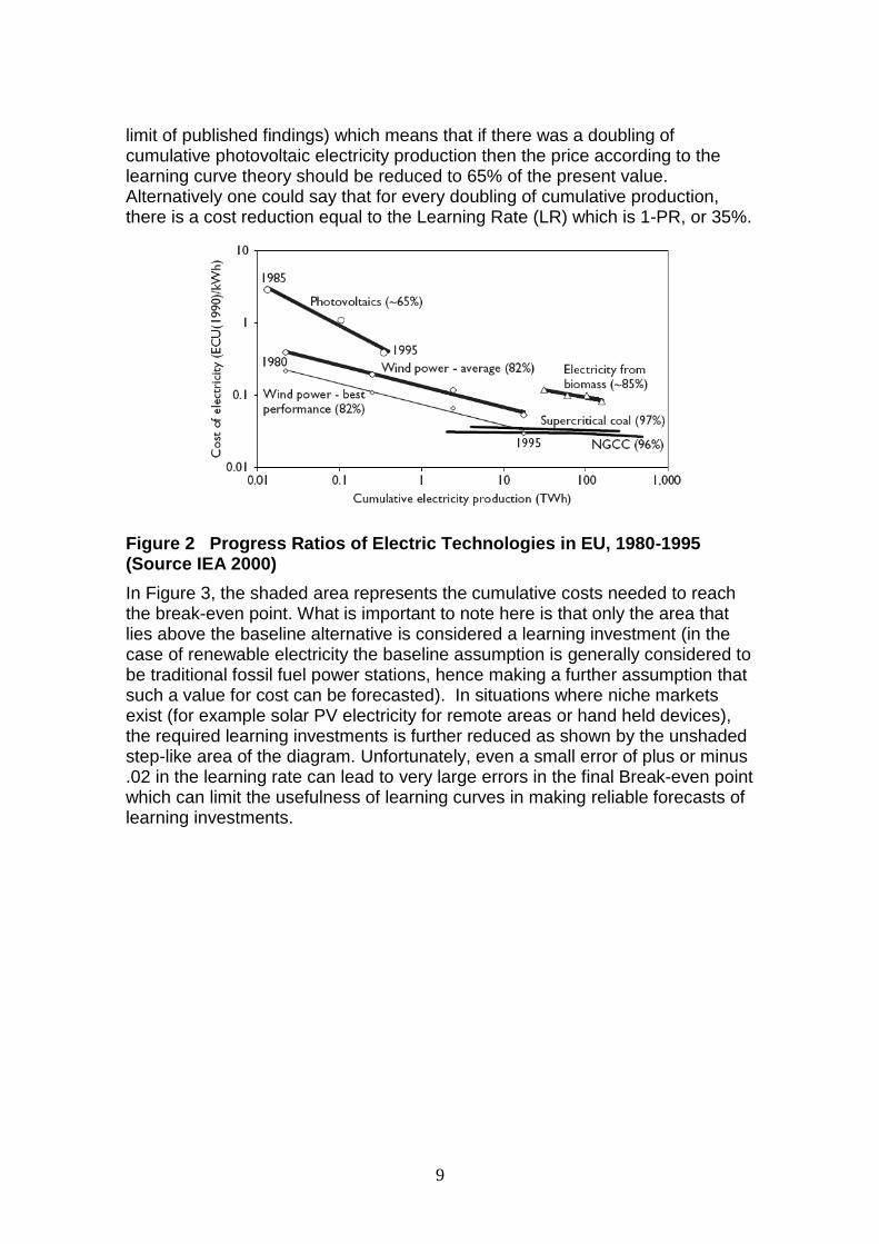
Figure 2 presents learning rates for a number of electricity producing technologies where electricity costs are shown in 1990 US dollars per kWh and are graphed against cumulative production in TWh. The graphic shows the lines of best fit on a log-log scale with associated progress ratios included. For each technology the linear slope shown is equal to the „-b‟ as described in Equation (2). This can also be transferred into a Learning Rate (LR) by using Equation (7). For example in this study, photovoltaics has a PR of 65% (the very upper

9

limit of published findings) which means that if there was a doubling of cumulative photovoltaic electricity production then the price according to the learning curve theory should be reduced to 65% of the present value. Alternatively one could say that for every doubling of cumulative production, there is a cost reduction equal to the Learning Rate (LR) which is 1-PR, or 35%.

Figure 2 Progress Ratios of Electric Technologies in EU, 1980-1995 (Source IEA 2000)

In Figure 3, the shaded area represents the cumulative costs needed to reach the break-even point. What is important to note here is that only the area that lies above the baseline alternative is considered a learning investment (in the case of renewable electricity the baseline assumption is generally considered to be traditional fossil fuel power stations, hence making a further assumption that such a value for cost can be forecasted). In situations where niche markets exist (for example solar PV electricity for remote areas or hand held devices), the required learning investments is further reduced as shown by the unshaded step-like area of the diagram. Unfortunately, even a small error of plus or minus .02 in the learning rate can lead to very large errors in the final Break-even point which can limit the usefulness of learning curves in making reliable forecasts of learning investments.

10

Figure 3 Cumulative learning investment requirements with different value niche markets (Schaeffer 2004 p18).

Not only has the standard SFLC been used, but a number of more complex versions have also been developed. One common example is the 2FLC which combines both „learning-by-doing‟ and „leaning-by-searching‟ that relates cost reductions to both cumulative experience and cumulative R&D as described in Equation (10).

c

t

b

t

tK

K

X

XPP

00

0

(10)

This presupposes that spending on R&D can also help achieve cost reductions, through all stages of a product‟s life cycle, and thus can become an important factor when forecasting the effects of, say, increasing R&D spending. There are, however, serious limitations on publicly available data about private R&D expenditure and so it can be very difficult to make an accurate representation of this factor (Junginger 2005). Lack of such data explains perhaps why the SFLC is often the preferred choice in technology modelling though it has also been suggested by some authors that R&D has only a minor and often statistically insignificant effect on costs when used with historical data. Papineau (2006) for example found the results of R&D “disappointing” for wind and solar production. She suggested that this may be due in part to the relative benefits of other forms of government intervention “such as direct subsidisation” that lead to increased cumulative production, rather than increases in R&D. Furthermore the relationship between R&D investment and cost reductions involve relatively long delays, which may go part way to explaining the lack of statistical evidence for the benefits of R&D investments. Rubin et al. (2004) also note that “cumulative production or capacity can be considered a surrogate for total accumulated knowledge gained from many different activities whose individual contributions cannot be readily discerned or modelled”. One explanation for some of the difficulty in arriving at accurate results for the 2FLC is a “„virtual cycle‟ or positive feedback loop between R&D, market growth and price reduction which stimulated its development” (Wanatabe 1999 in Barreto &

11

Kypreos 2004, p616). Here the authors concluded that “sound models for the role of R&D in the energy innovation system are not yet available” (Barreto & Kypreos 2004, p616).

When looking at learning in the wider environment as well as in firm specific situations, an important role is played by technology spillover effects. Here the learning mechanism is associated not just with learning of a single technology but instead the entire cluster of related technologies. Learning rates that incorporate spillovers within clusters of technologies have also been calculated and included in energy technology models (Gritsevski & Nakicenovic 2000). To what extent clustering technologies together can improve forecasts within the learning curve paradigm remains unclear due to added uncertainties that comes with the inclusion of other factors.

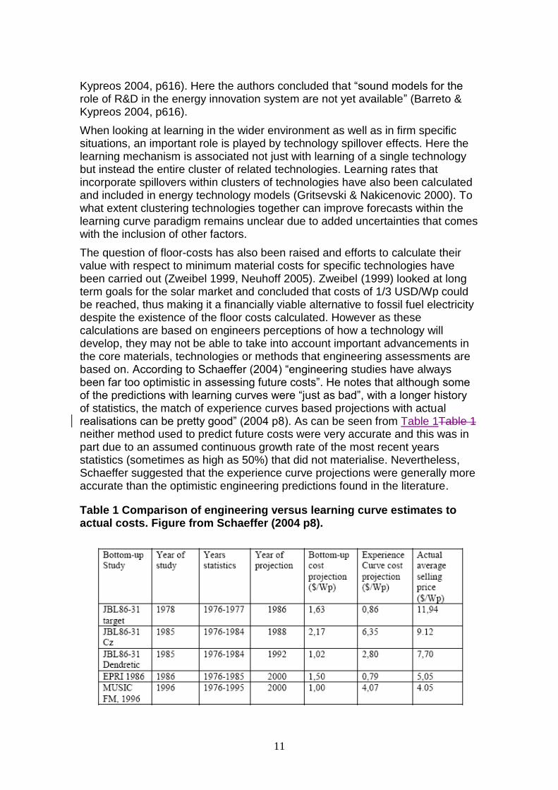
The question of floor-costs has also been raised and efforts to calculate their value with respect to minimum material costs for specific technologies have been carried out (Zweibel 1999, Neuhoff 2005). Zweibel (1999) looked at long term goals for the solar market and concluded that costs of 1/3 USD/Wp could be reached, thus making it a financially viable alternative to fossil fuel electricity despite the existence of the floor costs calculated. However as these calculations are based on engineers perceptions of how a technology will develop, they may not be able to take into account important advancements in the core materials, technologies or methods that engineering assessments are based on. According to Schaeffer (2004) “engineering studies have always been far too optimistic in assessing future costs”. He notes that although some of the predictions with learning curves were “just as bad”, with a longer history of statistics, the match of experience curves based projections with actual realisations can be pretty good” (2004 p8). As can be seen from Table 1Table 1 neither method used to predict future costs were very accurate and this was in part due to an assumed continuous growth rate of the most recent years statistics (sometimes as high as 50%) that did not materialise. Nevertheless, Schaeffer suggested that the experience curve projections were generally more accurate than the optimistic engineering predictions found in the literature.

Table 1 Comparison of engineering versus learning curve estimates to actual costs. Figure from Schaeffer (2004 p8).

12

Ongoing research has endeavoured to search ever deeper into the causes and agents of learning, far beyond the simple experience curves commonly found in the literature and many of the energy or E3 models. Generally the results of these more complex models can allow for a greater understanding of various technical factors relevant to the technology being tested (Nemet 2005, Coulomb & Neuhoff 2005, Mishina 1999). Nevertheless models based on technical factors suffer a limitation that experience curve models do not; they rely on intimate knowledge of the mechanisms leading to cost reductions. Although this makes perfect sense in terms of explaining past cost (or price) trends it may not be as valuable when trying to forecast future costs where new challenges may require unforeseen mechanisms that can not be endogenised into a technical factor model (as suggested by Coulomb & Neuhoff 2005). Furthermore such models would be difficult if not impossible to include in many E3 models due to their complexity and the lack of the required data within most models.

The heterogeneity of these and many other aspects of the innovation process is a reminder of the arbitrary nature of the learning curve paradigm. The unexplainable or unforeseen leaps and periods of stagnation or cost inflation visible in many learning curves studied only serve to remind us of the precarious reliance on learning curves found in many E3 models. This is true not only for assessing the costs associated with new technologies but also for forecasting the costs associated with existing technologies such as the requirement for SOx and NOx scrubbers in coal plants. This returns us once again to what has been asserted by various authors as the largest limitation to the use of experience curves: the need for more accurate data and the inherent uncertainty associated with the learning model itself (for instance Papineau 2004, IEA 2000). One approach to deal with this problem is to “incorporate stochastic learning curve uncertainty” directly into the model (Papineau 2004, p10), potentially reducing the dangers of using the learning curve method for forecasting. This research project aims to support the inclusion of stochastic modelling of learning by providing statistical data on the effectiveness of learning curves to forecast future technology costs.

3. A Statistical model for evaluating learning curve cost forecasting

Regression analysis has been used to test 3 hypotheses relating to the use of experience curves for forecasting technology costs (please note that prices have been used as a proxy for costs throughout). These are:

H1: Experience curves can be used as an unbiased estimator of future technology costs

H2: The ability to forecast technology costs improves as more data points are added

H3: Recent data is more important than older data for forecasting the cost of a specific technology

Hypothesis 1 was tested by considering the shape of the error distribution both in terms of mean deviation and skewness.

13

Hypothesis 2 was tested by comparing the distribution of the forecast errors using only the first half of the forecast data set to that using the second half.

Hypothesis 3 was tested using the Weighted Least Squares (WLS) regression function from Matlab and using exponentially increasing weights by 10% to 20% per year. Here an annual increase in the weighting factor of „w‟ percent has been used and a number of different values of this weighting factor „w‟ tested with the results for 10% and 20% presented here. Schaeffer (2004) proposed using weighting factors for the calculation of learning curves, however rather than weighting data according to the uncertainty in the cost/price estimate of each data point as he suggested, exponential weightings have been used to describe the (potential) reduced importance of older data as compared to newer data in explaining future costs of a given technology. There is also an important problem relating to data quality at the early stages of production, in particular due to the pricing strategies of companies. Forward selling for instance in the hope of creating a market and reaching desired cost levels or monopolistic behaviour aiming to cream profits and recover previous investments are 2 such examples. Although we have not endeavoured to account for such uncertainties in this paper, the development of criteria and weighting factors specific to these kind of problems could lead to more accurate results. Nevertheless by considering increasing weightings for newer data we are able to test the importance of earlier information as compared to more recent information for making long term forecasts.

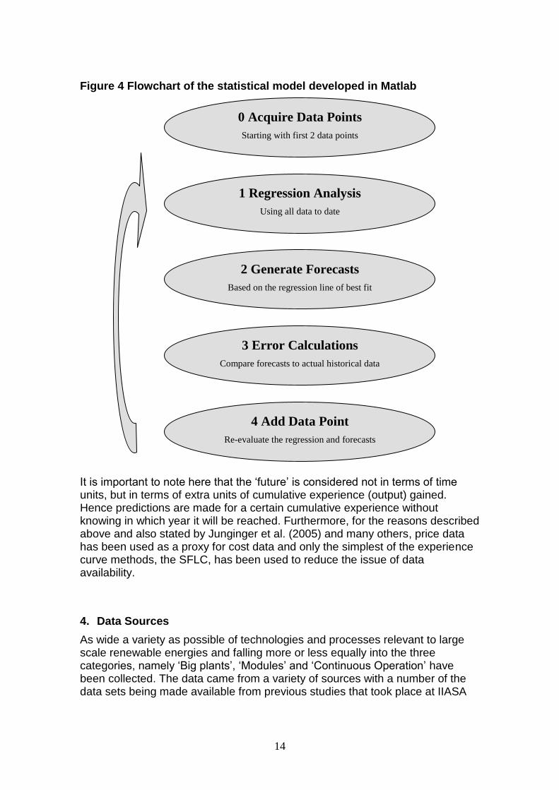
The steps of this model executed in Matlab can be summarised by the flowchart in Figure 4Figure 4. The regression analysis of step 1 has been undertaken using logarithmic base 2 of both price and cumulative output. In step 2, using the resulting learning curve, forecasts were made for one to six doublings of cumulative learning. The error of the forecast is calculated both in logarithmic terms, as well as calculating the percentage error in monetary units. Finally, each forecast has been compared to the actual historical data from which forecast error histograms are drawn. When comparing the forecasts to the historical data, simple linear interpolation has been used between future data points. Error has been calculated as a deviation from the forecasted value, such that a positive value indicates that the forecast was too low, while a negative value indicates that the forecast was too high. Finally another data point is added to the data series and forecasts are updated.

14

Figure 4 Flowchart of the statistical model developed in Matlab

It is important to note here that the „future‟ is considered not in terms of time units, but in terms of extra units of cumulative experience (output) gained. Hence predictions are made for a certain cumulative experience without knowing in which year it will be reached. Furthermore, for the reasons described above and also stated by Junginger et al. (2005) and many others, price data has been used as a proxy for cost data and only the simplest of the experience curve methods, the SFLC, has been used to reduce the issue of data availability.

4. Data Sources

As wide a variety as possible of technologies and processes relevant to large scale renewable energies and falling more or less equally into the three categories, namely „Big plants‟, „Modules‟ and „Continuous Operation‟ have been collected. The data came from a variety of sources with a number of the data sets being made available from previous studies that took place at IIASA

0 Acquire Data Points

Starting with first 2 data points

1 Regression Analysis

Using all data to date

2 Generate Forecasts

Based on the regression line of best fit

3 Error Calculations

Compare forecasts to actual historical data

4 Add Data Point

Re-evaluate the regression and forecasts

15

(McDonald & Schrattenholzer 2001). In general the raw data provided (in real monetary units) was used without any conversions, filtering or smoothing. One exception is the Combined Cycle Gas Turbine (CCGT) where data provided by Colpier was already converted from „costs per installed capacity‟ to „costs per electricity produced‟ (2002). The focus has been on technologies that remained in their growth stages in order to avoid problems associated with „forgetting by not doing‟ and where data for forecasting at least 3 doublings of technologies was available, the exception being nuclear where less data was available as shown in Table 2Table 2.

The result of using this selecting criteria has been that all of the technologies by their very inclusion are technologies that have had at least some degree of success. This selection bias means that the results may not be representative of all technologies. Furthermore, due to limited access to data and the selection criterion, the set of 12 technologies which combined allow for up to 130 individual short term forecasts (1 doubling of cumulative experience) can not be assumed to be representative of all technologies but does offer a number of highly relevant initial findings with regards to energy technology forecasting and modelling.

Table 2 Technology details and sources included in the study

Units

Initial

Year

Final

Year

Data

Points

Forecasted

doublings Source

CCGT Electricity Usc(90)/kWh - TWh 1981 1997 15 3.6 Cleason Colpier 2002

Nuclear Instalation US$(90)/W - GW 1975 1993 19 2.0Kouvaritakis et al. (2000) in M&S

2001

SCGT Instalation US$(90)/W - GW 1956 1981 14 8.9 IIASA-WEC (1998), p.50

Solar Production $/Wp - MWp 1975 2003 29 9.6 Maycock (2005)

Sony Laser Diode Production yen - 1000*units 1982 1994 13 13.3Lipman and Sperling (1999) in

M&S 2001

Ford Model-T Shipments$(58)/unit - Million

units199 213 12 7.3

Abernathy and Wayne (1974), in

M&S 2001

Average Dram MBit Production $/Mbit - Mbit 1974 1998 25 20.6 Victor & Ausubel (????)

Ethanol Production $/GJ-GJ 1980 2004 25 5.3 Goldemberg et al. (2004)

Acrylonitrile Production $(66)/unit - units 1959 1972 14 3.0 Lieberman (1984)

Polyethylene-LD Production $(66)/unit - units 1958 1972 15 3.5 Lieberman (1984)

Polyethylene-HD Production $(66)/unit - units 1958 1972 15 3.9 Lieberman (1984)

Polyester Fibers Production $(66)/unit - units 1960 1972 13 4.4 Lieberman (1984)

Big plants

Modules

Continuous

Operation

Technology type

16

5. Results

As well as the aggregated results presented in the final subsection, 3 individual case studies of particular relevance to energy and renewable energy technologies will initially be presented in detail. Each case study comes from one of the three technology groups as set out by Christiansson (1995), namely „continuous operation‟, „modules‟ and „big plants‟.

Continuous operation case study – Brazilian Ethanol

Although Brazilian ethanol production may not be the most general example of a “continuous operation” technology, it does provide a valuable case study for evaluating the effectiveness of learning by doing as a mechanism for a technology to reach cost effectiveness. It may also be considered as one of the few large scale renewable energy technologies that has been able to reach cost effectiveness. For each technology the output graphics use the lightest lines to represent the learning curve made with fewer data points and the darkest lines with the largest set of data points. In the case of Ethanol in Figure 5Figure 5, it can be seen that the slope of the learning curve has mostly increased as experience has been gained. The 4 individual graphics represent the 4 methods modelled, namely OLS, WLS where the weightings are exponentially increasing by 10% and 20% per year and finally RLS.

Figure 5 Log-log representation of learning curve fit to Brazilian ethanol data using various methods

As one would expect for WLS with exponentially increasing weightings, the later predictions represented by the darker lines are able to follow more closely the

17

trend of Ethanol to become cheaper faster than the initial experience curve projected. The curve for ethanol also shows many of the non-linear characteristics as has been demonstrated in the literature such as the “deviations from log-linearity at the beginning and tail of the curve” (Antes, Yeh & Berkenpas 2005; p7), however this effect was not generally systematic across technologies. Despite these deviations it can be seen when looking at the non-linear graphical representation (using standard format rather than log-log format as shown in Figure 6Figure 6), that even during this earlier period very significant cost reductions took place.

Figure 6 Non-linear representation of learning curve fit to Brazilian ethanol data using OLS and Weighted LS methods

Finally, in the case for Ethanol an excellent opportunity exists for the consideration of the relative effectiveness of these methods to determine the learning investment required to reach the price level of an incumbent technology. Here an approximate price level of the non-renewable energy that it replaces, petrol has been used as the incumbent price level. The “learning investments” required for the technology to reach break-even has been calculated by integrating the extra costs that lie between the horizontal incumbent technology baseline and the actual data of the price paid to ethanol producers and forecasts thereof as shown in Figure 6Figure 6. To calculate the entire forecasted learning investment required, historical values are used to calculate the investments to date and then the difference between the learning curve forecast and the baseline has been integrated to determine future learning investments required to reach break-even.

18

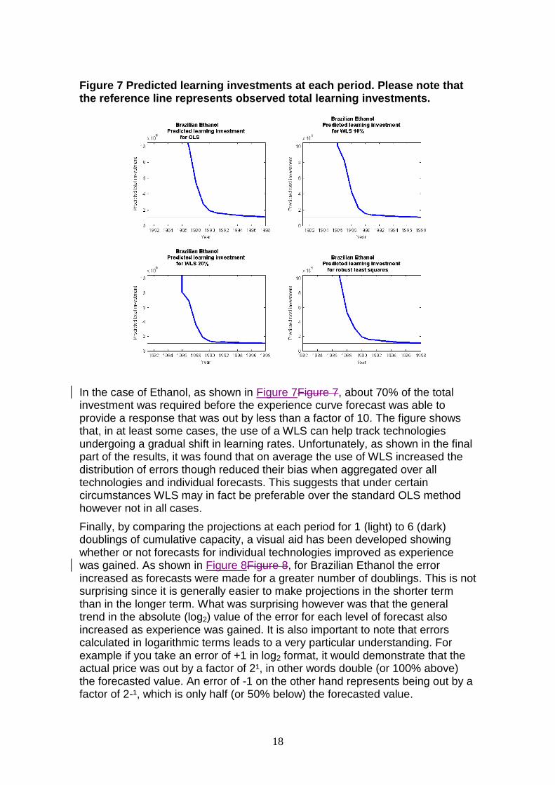
Figure 7 Predicted learning investments at each period. Please note that the reference line represents observed total learning investments.

In the case of Ethanol, as shown in Figure 7Figure 7, about 70% of the total investment was required before the experience curve forecast was able to provide a response that was out by less than a factor of 10. The figure shows that, in at least some cases, the use of a WLS can help track technologies undergoing a gradual shift in learning rates. Unfortunately, as shown in the final part of the results, it was found that on average the use of WLS increased the distribution of errors though reduced their bias when aggregated over all technologies and individual forecasts. This suggests that under certain circumstances WLS may in fact be preferable over the standard OLS method however not in all cases.

Finally, by comparing the projections at each period for 1 (light) to 6 (dark) doublings of cumulative capacity, a visual aid has been developed showing whether or not forecasts for individual technologies improved as experience was gained. As shown in Figure 8Figure 8, for Brazilian Ethanol the error increased as forecasts were made for a greater number of doublings. This is not surprising since it is generally easier to make projections in the shorter term than in the longer term. What was surprising however was that the general trend in the absolute (log2) value of the error for each level of forecast also increased as experience was gained. It is also important to note that errors calculated in logarithmic terms leads to a very particular understanding. For example if you take an error of +1 in log2 format, it would demonstrate that the actual price was out by a factor of 2¹, in other words double (or 100% above) the forecasted value. An error of -1 on the other hand represents being out by a factor of 2-¹, which is only half (or 50% below) the forecasted value.

19

Furthermore as prices come down forecast errors need to come down proportionally in order to maintain constant logarithmic error.

Figure 8 Forecast error (log2) as a function of (log2) cumulative production. Note that the robust least squares method requires 3 data points to make the first line of best fit reducing the number of forecasts possible

Big plants case study – CCGT

The data set for CCGT originally came from a reduced list of over 200 published contract costs in trade journals for new CCGT plants (Colpier & Cornland 2002). The data was then converted from cost per MW of installed capacity to cost per kWh of produced electricity holding gas costs constant. The main reason for this conversion was that CCGT cost reductions were often traded off against more expensive quality and efficiency improvements. CCGT operators are generally interested in the reduction of the cost of producing electricity and not simply the reduction of installation costs making the former a more relevant dependant variable.

20

Figure 9 Technology price (solid) and Annual Production Growth (dashed) for CCGT energy production.

Figure 10 Experience curves for CCGT using cost of energy production with constant gas costs versus cumulative energy produced.

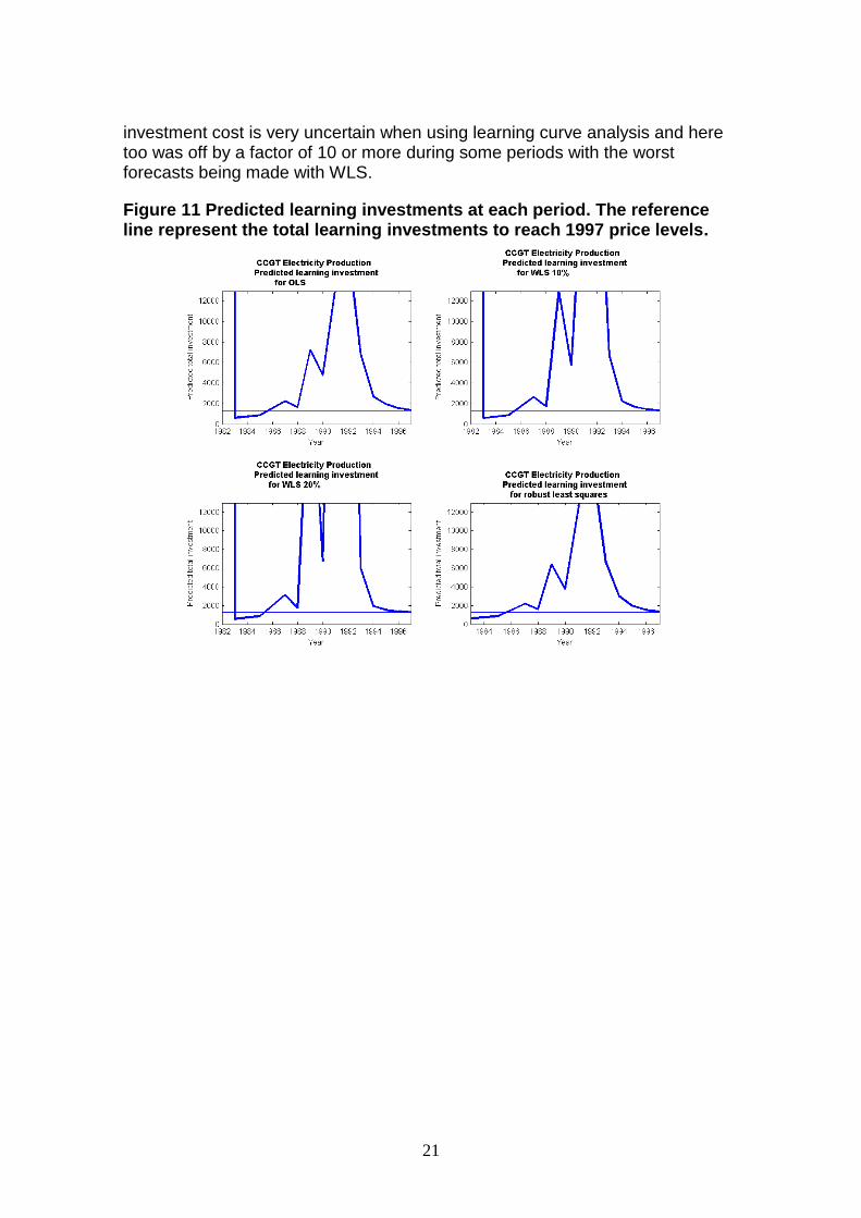
From Figure 10Figure 10 we see a case where the use of WLS has generated a wider range of learning curve results which in the end seemed to have proved less effective than the standard OLS method. Furthermore, as shown in Figure 11Figure 11 where we have assumed a target price of the 1997 value of 3.37 USc(1990)/kWh, it was found that the forecasted cumulative learning

21

investment cost is very uncertain when using learning curve analysis and here too was off by a factor of 10 or more during some periods with the worst forecasts being made with WLS.

Figure 11 Predicted learning investments at each period. The reference line represent the total learning investments to reach 1997 price levels.

22

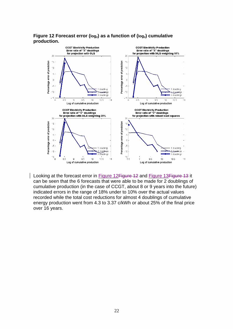
Figure 12 Forecast error (log2) as a function of (log2) cumulative production.

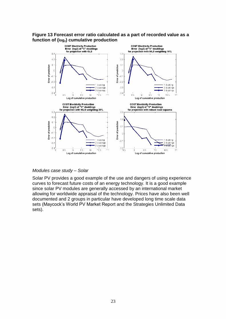
Looking at the forecast error in Figure 12Figure 12 and Figure 13Figure 13 it can be seen that the 6 forecasts that were able to be made for 2 doublings of cumulative production (in the case of CCGT, about 8 or 9 years into the future) indicated errors in the range of 18% under to 10% over the actual values recorded while the total cost reductions for almost 4 doublings of cumulative energy production went from 4.3 to 3.37 c/kWh or about 25% of the final price over 16 years.

23

Figure 13 Forecast error ratio calculated as a part of recorded value as a function of (log2) cumulative production

Modules case study – Solar

Solar PV provides a good example of the use and dangers of using experience curves to forecast future costs of an energy technology. It is a good example since solar PV modules are generally accessed by an international market allowing for worldwide appraisal of the technology. Prices have also been well documented and 2 groups in particular have developed long time scale data sets (Maycock‟s World PV Market Report and the Strategies Unlimited Data sets).

24

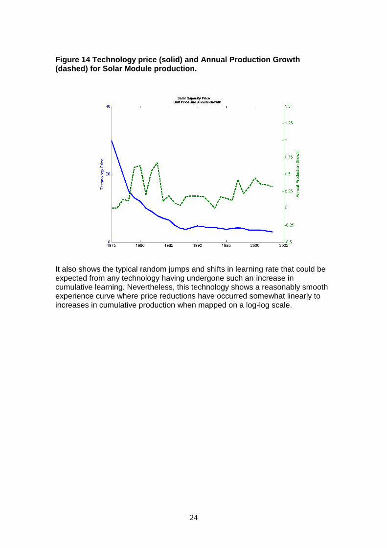
Figure 14 Technology price (solid) and Annual Production Growth (dashed) for Solar Module production.

It also shows the typical random jumps and shifts in learning rate that could be expected from any technology having undergone such an increase in cumulative learning. Nevertheless, this technology shows a reasonably smooth experience curve where price reductions have occurred somewhat linearly to increases in cumulative production when mapped on a log-log scale.

25

Figure 15 Log-log representation of learning curve fit to solar PV module price data using various methods. Note that solar has not yet reached large scale competitivity, the price level used as a baseline of 1$/Wp has been arbitrarily chosen. Such a price level would greatly increase the number of competitive applications if not allow PV to become completely cost effective.

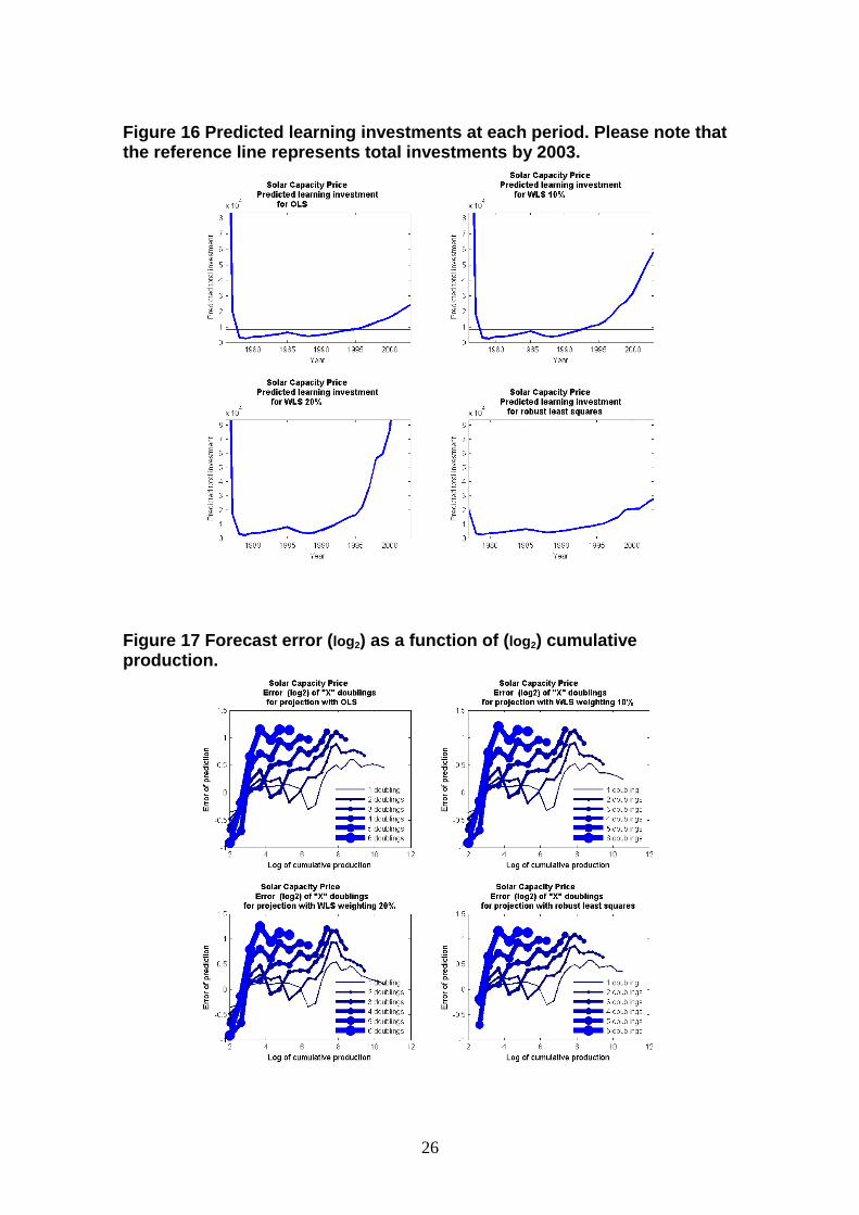
Figure 16Figure 16 and Figure 15Figure 15 together present an interesting result of the use of exponentially increasing weights. Since the experience curve slope reduces over the period of the data set, the WLS method was able to track the change in learning rate making the forecasts for total learning investments more accurately than the standard OLS method. Unfortunately it remained difficult or impossible to know from the limited data available whether the shift to a lower learning rate was indeed a permanent shift or merely a period of stagnation. Using the simple experience curve based model described in this research, it has been possible to make a statistical evaluation of how effective different methods have been in the past over a range of technologies to help advise which method tends to work best on average. These results are presented in the following sub-section on aggregated results.

26

Figure 16 Predicted learning investments at each period. Please note that the reference line represents total investments by 2003.

Figure 17 Forecast error (log2) as a function of (log2) cumulative production.

27

Aggregated results for experience curve forecasts

In this section the various experience curve formulation and their ability to forecast into the future are compared by consolidating the forecast errors for each number of doublings into the future all onto a single graphic as shown in Figure 18Figure 18.

Figure 18 Histogram of the log of the errors over all technologies and for the forecast at every period of each technology where available historical data exists for 1 doubling of cumulative experience

This first example offers the most reliable information with the largest number of data points available allowing for what turns out to be a reasonably smooth distribution. Unfortunately, a single doubling of experience referred typically to somewhere in the region of 2 to 6 years depending on the growth rate of the technology in question. It also depended on the stage that the technology was in since the time taken to generate a doubling of experience increases as the stock of cumulative experience also increases, even when the growth rate of a technology remains constant. What the graphical representation of the data does show is that the forecast error in log format is a very good first order approximation with the distribution being both symmetrical and unbiased with a mean value that is statistically not different from zero for both the OLS and WLS methods. It is also interesting to note that the OLS method offered the best results in terms of mean deviation of forecast error and as such is the least biased estimator of future costs in the short term while the overall error in terms of standard deviation was slightly reduced when using the WLS method.

28

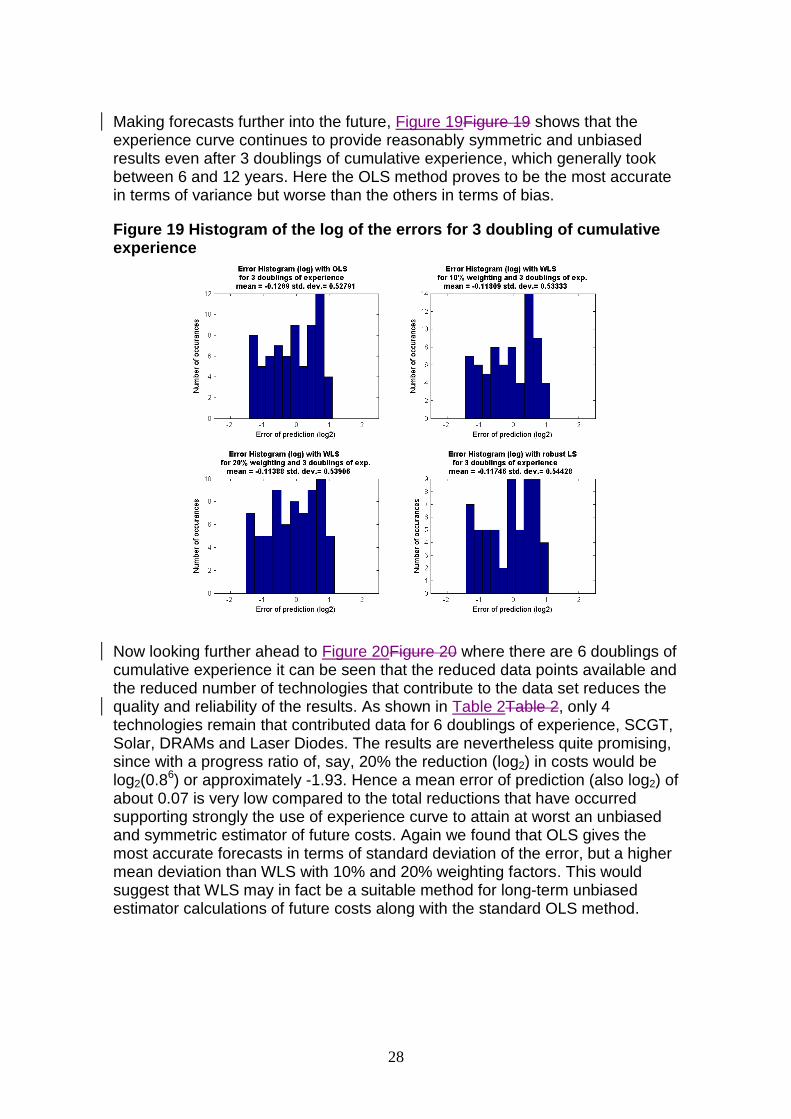
Making forecasts further into the future, Figure 19Figure 19 shows that the experience curve continues to provide reasonably symmetric and unbiased results even after 3 doublings of cumulative experience, which generally took between 6 and 12 years. Here the OLS method proves to be the most accurate in terms of variance but worse than the others in terms of bias.

Figure 19 Histogram of the log of the errors for 3 doubling of cumulative experience

Now looking further ahead to Figure 20Figure 20 where there are 6 doublings of cumulative experience it can be seen that the reduced data points available and the reduced number of technologies that contribute to the data set reduces the quality and reliability of the results. As shown in Table 2Table 2, only 4 technologies remain that contributed data for 6 doublings of experience, SCGT, Solar, DRAMs and Laser Diodes. The results are nevertheless quite promising, since with a progress ratio of, say, 20% the reduction (log2) in costs would be log2(0.86) or approximately -1.93. Hence a mean error of prediction (also log2) of about 0.07 is very low compared to the total reductions that have occurred supporting strongly the use of experience curve to attain at worst an unbiased and symmetric estimator of future costs. Again we found that OLS gives the most accurate forecasts in terms of standard deviation of the error, but a higher mean deviation than WLS with 10% and 20% weighting factors. This would suggest that WLS may in fact be a suitable method for long-term unbiased estimator calculations of future costs along with the standard OLS method.

29

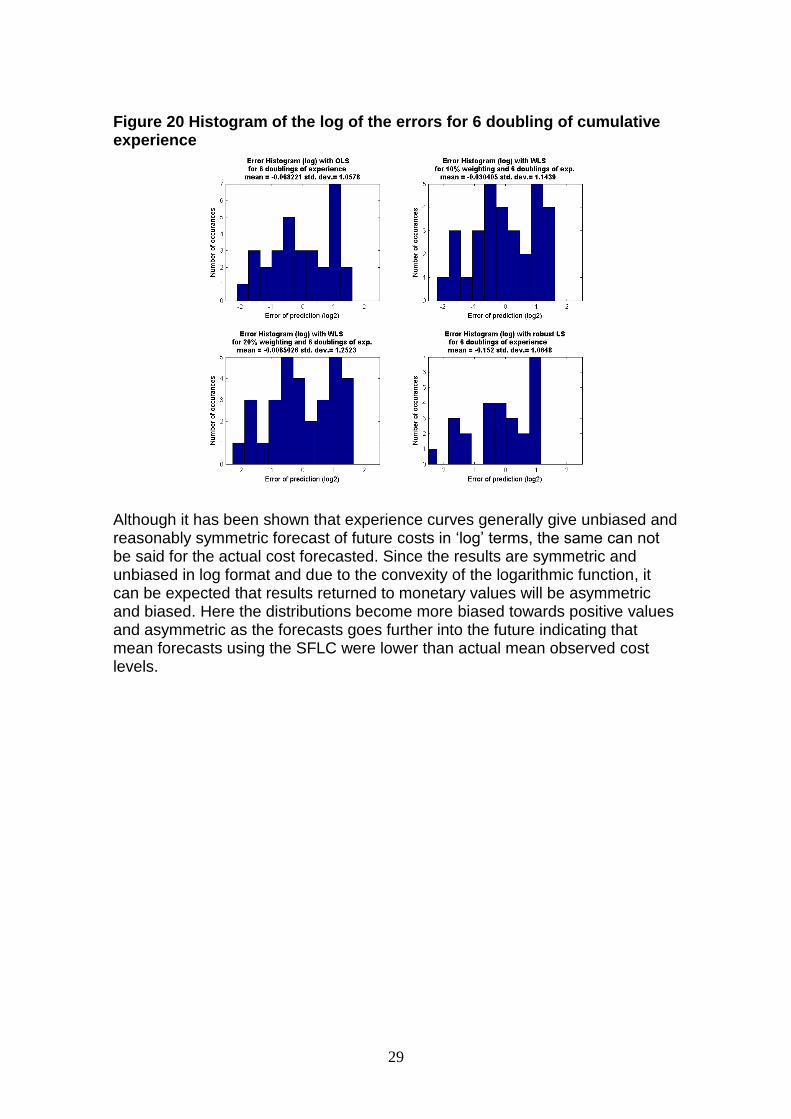
Figure 20 Histogram of the log of the errors for 6 doubling of cumulative experience

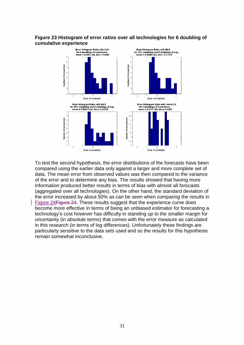
Although it has been shown that experience curves generally give unbiased and reasonably symmetric forecast of future costs in „log‟ terms, the same can not be said for the actual cost forecasted. Since the results are symmetric and unbiased in log format and due to the convexity of the logarithmic function, it can be expected that results returned to monetary values will be asymmetric and biased. Here the distributions become more biased towards positive values and asymmetric as the forecasts goes further into the future indicating that mean forecasts using the SFLC were lower than actual mean observed cost levels.

30

Figure 21 Histogram of error ratios over all technologies for 1 doubling of cumulative experience

Figure 22 Histogram of error ratios over all technologies for 3 doubling of cumulative experience

31

Figure 23 Histogram of error ratios over all technologies for 6 doubling of cumulative experience

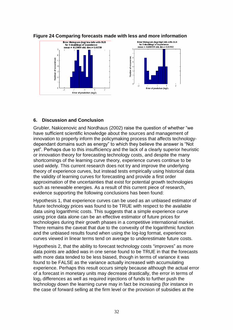
To test the second hypothesis, the error distributions of the forecasts have been compared using the earlier data only against a larger and more complete set of data. The mean error from observed values was then compared to the variance of the error and to determine any bias. The results showed that having more information produced better results in terms of bias with almost all forecasts (aggregated over all technologies). On the other hand, the standard deviation of the error increased by about 50% as can be seen when comparing the results in Figure 24Figure 24. These results suggest that the experience curve does become more effective in terms of being an unbiased estimator for forecasting a technology‟s cost however has difficulty in standing up to the smaller margin for uncertainty (in absolute terms) that comes with the error measure as calculated in this research (in terms of log differences). Unfortunately these findings are particularly sensitive to the data sets used and so the results for this hypothesis remain somewhat inconclusive.

32

Figure 24 Comparing forecasts made with less and more information

6. Discussion and Conclusion

Grubler, Nakicenovic and Nordhaus (2002) raise the question of whether “we have sufficient scientific knowledge about the sources and management of innovation to properly inform the policymaking process that affects technology-dependant domains such as energy” to which they believe the answer is “Not yet”. Perhaps due to this insufficiency and the lack of a clearly superior heuristic or innovation theory for forecasting technology costs, and despite the many shortcomings of the learning curve theory, experience curves continue to be used widely. This current research does not try and improve the underlying theory of experience curves, but instead tests empirically using historical data the validity of learning curves for forecasting and provide a first order approximation of the uncertainties that exist for potential growth technologies such as renewable energies. As a result of this current piece of research, evidence supporting the following conclusions has been found:

Hypothesis 1, that experience curves can be used as an unbiased estimator of future technology prices was found to be TRUE with respect to the available data using logarithmic costs. This suggests that a simple experience curve using price data alone can be an effective estimator of future prices for technologies during their growth phases in a competitive international market. There remains the caveat that due to the convexity of the logarithmic function and the unbiased results found when using the log-log format, experience curves viewed in linear terms tend on average to underestimate future costs.

Hypothesis 2, that the ability to forecast technology costs “improves” as more data points are added was in one sense found to be TRUE in that the forecasts with more data tended to be less biased, though in terms of variance it was found to be FALSE as the variance actually increased with accumulating experience. Perhaps this result occurs simply because although the actual error of a forecast in monetary units may decrease drastically, the error in terms of log2 differences as well as required injections of funds to further push the technology down the learning curve may in fact be increasing (for instance in the case of forward selling at the firm level or the provision of subsidies at the

33

government level). Finally, as can be seen for most technologies, the distance between data values on the quantity axis gets closer and closer together as a technology matures since every doubling of experience requires more and more time. Along with this added time requirement one would also expect the possibility of increased uncertainty. Access to a larger representative database would certainly help to bring more concrete results in particular with respect to this hypothesis.

Hypothesis 3, that the use of exponentially increasing weights when using weighted least squares allows for improved accuracy of predictions turned out to be in one sense TRUE and in one sense FALSE. It was found that over all the technologies tested, the use of WLS generally increased the variance of the forecasts as compared to the OLS method but decreased the mean deviation or „bias‟ of the forecast. This would suggest that although the standard OLS method is a highly effective predictor of future costs/costs, there may be opportunities for WLS to be a superior method for producing these experience curves.

One of the principal difficulties with informing policy makers on how best to bring about cost reductions of renewable energy technologies is to decide how to divide a limited budget so that it is concentrated enough to bring about desired cost reductions of a chosen technology while being broad enough to offer a range of possible technical solutions in the case that the technologies first picked as winners turn out to be undesirable or unsuccessful (one only needs to think of the public resistance to on shore wind farms in the UK and elsewhere). As remarked by Wene in his IEA publications. “learning opportunities in the market and learning investments are both scarce resources” suggesting that the concentration of resources is key to generating solutions, whilst on the other hand, the “availability of renewable resources, reliability of the energy system and the risk of technology failure require a portfolio of carbon-free technologies” (IEA 2000, IIASA approach, see, e.g. Gritsevski & Nakicenovic 2000). In this paper the distributions of forecasted technology price errors haves been calculated based on historical data, allowing future portfolio research to take this information into account when designing energy technology portfolios.

A great deal more work needs to follow in this area in order to increase our understanding of the evolution of technology costs. For example, improving data quality and increasing the number and scope of technologies tested using a similar analysis would help provide more accurate results. It may also be important to consider the importance of autocorrelation to allow for better forecasts and simulations of future technology costs. Data permitting it would be very interesting to test other formulations such as the 2FLC or methods that account for technology clusters for their ability to improve forecast quality. Finally, investigating the circumstances and criterion where the use of WLS would be preferred over the standard OLS would also constitute an interesting area for further research.

34

References

[1] Antes, M., Yeh, S., Berkenpas, M. 2005 Estimating future trends in the cost of CO2 capture technologies, Final report to IEA GHG R&D Program.

[2] Arrow, K, 1962, „The economic implications of Learning by Doing‟, Review of Economic Studies, vol. 29, pp155-173.

[3] Barreto, L. & Kypreos, S., 2004, „Emissions trading and technology deployment in an energy-systems “bottom-up” model with technology learning‟, European journal of operational research, vol. 158, pp 243-261.

[4] Carraro, C. & Hourcade, J., 1998, „Climate modelling and policy strategies. The role of technical change and uncertainty‟, Energy Economics, 20, pp 463-471

[5] Christiansson, L., 1995, Diffusion and Learning Curves of Renewable Energy Technologies, IIASA working paper series WP-95-126.

[6] Coulomb, L. & Neuhoff, K. 2005 Learning curves and changing product attributes: the case of wind turbines, Cambridge University working paper series EPRG 0601.

[7] Colpier, U. & Cornland, D., 2002, The economics of the combined cycle gas turbine-an experience curve analysis, Energy Policy 30 pp 309-322.

[8] Everett, J. & Farghal, S. 1994 Learning curve predictors for construction field operations, Journal of construction engineering and management.

[9] Everett, J. & Farghal, S. 1997 Data representation for predictive performance with learning curves, Journal of construction engineering and management.

[10] Farghal, S. & Everett, J. 1997 Learning Curves: Accuracy in predicting future performance, Journal of construction engineering and management.

[11] Goldemberg, J., Coelho, S., Nastari, P. & Lucon, O. 2004 Ethanol learning curve – the Brazilian experience, Biomass & Bioenergy 26 pp301-304

[12] Gritsevski, A. & Nakicenovic, N. 2000 Modelling uncertainty of induced technical change, Energy Policy 28, pp907-921

[13] Grübler, A. & Messner, S, 1998, „Technological change and the timing of mitigation measures‟, Energy Economics, 20, pp 495-512

35

[14] Gruebler, A., Nakicenovic, N. & Nordhaus WD. (Eds) 2002 Technological Change and the Environment, Resources for the Future, Washington, DC, USA [2002] [ISBN 1-891853-46-5]

[15] Henderson, Bruce, 1973a, „The experience curve reviewed – II. History‟, BCG, No 125. www.bcg.com.

[16] Henderson, Bruce, 1973b, „The experience curve reviewed – IV‟. The growth share matrix, BCG, No 149. www.bcg.com.

[17] IEA, 2000, „Experience Curves for Energy Technology Policy‟, IEA Paris, France.

[18] Irwin, D. & Klenow, P., 1994, Learning-by-Doing Spillovers in the Semiconductor Industry, The journal of Political Economy Vol 102 No. 6 pp1200-1227.

[19] Junginger, M et al., 2005, „Global experience curves for wind farms‟, Energy Policy, vol. 33, pp 133–150

[20] Lieberman, M., 1984, The learning curve and pricing in the chemical processing industry, The Rand Journal of Economics Vol. 15, No.2 pp213-228

[21] Lieberman, M., 1987, „The learning curve, diffusion, and competitive strategy‟, Strategic Management Journal, vol. 8, pp 441-452

[22] Maycock, P. 2005 PV REVIEW: World Solar PV Market Continues Explosive Growth, ReFOCUS Sep/Oct

[23] McDonald, A., & Schrattenholzer, L., 2001, Learning rates for energy technologies, Energy Policy 29 pp 255-261

[24] Mishina, K., 1999, "Learning by New Experiences: Revisiting the Flying Fortress Learning Curve", in Lamoreaux, N., Raff, D. M. G. and Temin, P. (eds), Learning by Doing in Markets, Firms, and Countries, University of Chicago Press, Chicago.

[25] Papineau, 2006, „An economic perspective on experience curves and dynamic economies in renewable energy technologies‟, Energy Policy.

[26] Neuhoff, K., 2005, „Large Scale Deployment of Renewables for Electricity Generation‟, Oxford Review of Economic Policy, vol. 21 no. 1

[27] Rubin, Yeh & Hounshell, 2004, „Learning curves for environmental technology and their importance for climate policy analysis‟, Energy, 29 pp1551-1559.

[28] Schaeffer, G. (Ed) 2004 Photovoltaic power development: assessment of strategies using experience curves (acronym PHOTEX), Synthesis

36

report, Energy research centre of the Netherlands (ECN), Accessed via http://www.energytransition.info/photex/docs/synthesisreport.pdf on 3/8/06

[29] Victor, N. & Ausubel, J. 2002 DRAM‟s as model organisms for study of technological evolution, Technological forecasting and social change, Volume 69, Issue 3

[30] Zweibel, K., 1999, “Issues in thin film PV manufacturing cost reduction,” Solar Energy Materials & Solar Cells.