forecasting realized exchange rate volatility by decomposition

sting 23 (2007) 307–320www.elsevier.com/locate/ijforecast

International Journal of Foreca

Forecasting realized exchange rate volatility by decomposition

Markku Lanne ⁎

Department of Economics, P.O. Box 17 (Arkadiankatu 7), FI-00014 University of Helsinki, RUESG and HECER, Finland

Abstract

We compare forecasts of the realized volatility of the exchange rate returns of the Euro against the U.S. Dollar and theJapanese Yen obtained both directly and through decomposition. Decomposing the realized volatility into its continuous samplepath and jump components, and modeling and forecasting them separately instead of directly forecasting the realized volatility,is shown to lead to improved out-of-sample forecasts. Moreover, the gains in forecast accuracy are fairly robust with respect tothe details of the decomposition, but the jump component should probably not be defined too tightly.© 2007 International Institute of Forecasters. Published by Elsevier B.V. All rights reserved.

Keywords: Realized volatility; Mixture of distributions; Aggregation; Jumps; Exchange rates

1. Introduction

Recently, Andersen, Bollerslev, and Diebold (inpress) suggested modeling and forecasting the realizedvolatility of exchange rate, stock and bond returns byextracting the component due to jumps and including itas an explanatory variable in the heterogenous auto-regressive (HAR) regression model of Müller et al.(1997) and Corsi (2003). In some cases, the jumpcomponent turned out to be highly significant, andconsiderable increases in the coefficient of determinationwere observed. This suggests that gains in forecastingthe realized volatility could be made by separatelymodeling and forecasting the jump and continuoussample path components, and obtaining forecasts of therealized volatility as their sum instead of considering the

⁎ Tel.: +358 9 191 28731; fax: +358 9 191 28736.E-mail address: [email protected].

0169-2070/$ - see front matter © 2007 International Institute of Fdoi:10.1016/j.ijforecast.2007.02.001

orecaste

aggregate realized volatility, as conjectured byAndersenet al. (in press). The purpose of this paper is to studywhether such an approach really would be beneficial andwhether the potential gains in forecast accuracy dependon the way the decomposition is carried out. To this end,we examine the returns of the Euro against the U.S.Dollar and Japanese Yen (EUR/USD and EUR/YENreturns henceforth). To model the realized volatility andthe continuous components, we use the mixturemultiplicative error model (mixture-MEM henceforth)previously shown by Lanne (2006) to fit well tocomparable exchange rate data. One benefit of thismodel is that it cannot produce negative forecasts, unlikethe HAR regression model used by Andersen et al. (inpress). The jump components are modeled by means ofthe standardMarkov-switching model. While the resultsfor the two exchange rate volatility series are remarkablysimilar, there are also some notable differences.

The potential improvement in forecast accuracy dueto decomposition can be seen to result from two factors.

rs. Published by Elsevier B.V. All rights reserved.

mailto:[email protected]

http://dx.doi.org/10.1016/j.ijforecast.2007.02.001

308 M. Lanne / International Journal of Forecasting 23 (2007) 307–320

First, once the variation due to jumps has beeneliminated from the realized volatility series, theprocess of the remaining continuous sample pathcomponent may be more easily captured, i.e., itsprocess may be more easily estimable. Second, thejump component itself may contain predictable varia-tion that contributes toward the forecast of the realizedvolatility. We show that, at least with these data,statistically significant gains in out-of-sample forecastaccuracy can be made by decomposing, and thisfinding is fairly robust with respect to the details of thedecomposition. However, if the jump component isvery tightly defined, i.e., it takes nonzero values ononly the days with the very greatest jumps, it has verylittle predictable variation so that virtually all the gainsin forecast accuracy come from the improvements inestimating the process of the continuous component,causing somewhat less accurate forecasts at the one-day horizon. This finding extends the results ofAndersen et al. (in press), which defined the jumps asbeing the very largest ones. By building a model forthe jump component, we are able to forecast at longerhorizons, in contrast to Andersen et al. (in press), andour results demonstrate gains in accuracy in that case aswell. Although the results are clear in showing thebenefits of the decomposition, the diagnostic testssuggest that as far as the jump component is concerned,even further improvements might be attainable by theuse of more sophisticated models. While the results arein a sense specific to the chosen econometric models,they should be rather general, in that the mixture-MEMmodel has previously been shown to fit comparableexchange rate data at least as well as relevantalternatives in the literature, and diagnostic checkshere also indicate its adequacy.

The plan of the paper is as follows. In Section 2 thedecomposition methods put forth by Andersen et al. (inpress) are reviewed and applied to the EUR/USD data.In Section 3 the mixture-MEM and Markov-switchingmodels are introduced and the estimation results arereported, while the forecast comparisons are presentedin Section 4. Finally, Section 5 concludes.

2. Decomposition of realized volatility

In this section we discuss different decomposi-tions of the daily return variance, and introduce thedata set. As a starting point for the analysis we have

the realized variance of discretely sampled Δ-periodreturns rt,Δ≡p(t)−p(t−Δ),

RVtþ1ðDÞuX1=D

j¼1

r2tþjD;D; ð1Þ

where p(t) is the price of the asset at time point t. AsBarndorff-Nielsen and Shephard (2004) have shown,the difference between this measure and the stan-dardized realized bi-power variation,

BVtþ1ðDÞul−21X1=D

j¼2

jrtþjD;Djjrtþð j−1ÞD;Dj

where l1uffiffiffiffiffiffiffiffi2=p

p, consistently estimates the compo-

nent of the total return variation due to discrete jumps.Hence, it is natural to base the decomposition of RVt+1

(Δ) on RVt+1(Δ)−BVt+1(Δ). As this difference can alsotake negative values, the measure

Jtþ1ðDÞumax½RVtþ1ðDÞ−BVtþ1ðDÞ; 0� ð2Þ

suggested byBarndorff-Nielsen and Shephard (2004) canbe used instead to ensure the non-negativity of the jumpcomponent. The continuous sample path component Ct+1

(Δ) simply equals RVt+1(Δ)−Jt+1(Δ).One potential problem with Jt+1(Δ) is that it

typically takes positive values too frequently to becharacterized as a component due to jumps. Instead,it might be desirable to identify only the significantjumps. To this end, Andersen et al. (in press) suggestemploying the following test statistic

Ztþ1ðDÞuD−1=2 ½RVtþ1ðDÞ−BVtþ1ðDÞ�RVtþ1ðDÞ−1

fðl−41 þ 2l−21 −5Þmax½1;TQtþ1ðDÞBVtþ1ðDÞ�2�g1=2ð3Þ

the distribution of which Huang and Tauchen (2005)find to be approximated by the standard normaldistribution. Here, TQt+1(Δ) is the standized realizedtri-power quarticity,

TQtþ1ðDÞuD−1l−34=3X1=D

j¼3

jrtþjD;Dj4=3jrtþð j−1ÞD;Dj4=3jrtþð j−2ÞD;Dj4=3;

where μ4 / 3≡22 / 3Γ (7 /6)Γ (1 /2)−1 and Γ (·) is thegamma function. The idea is that the jump componentdefined by confidence level α, Jt+1,α(Δ), takes positive

309M. Lanne / International Journal of Forecasting 23 (2007) 307–320

values only on days on which the above test statistic issignificant, and equals zero otherwise, i.e.,

Jtþ1;aðDÞuI ½Ztþ1ðDÞNUa�½RVtþ1ðDÞ−BVtþ1ðDÞ�; ð4Þ

where I(·) denotes the indicator function and Φα is thecritical value at the confidence level α. This means thatthe definition of Jt+1,α(Δ) depends on the chosenconfidence level, or in other words, on what sizejumps are considered significant. In order to make surethat the components sum to RVt+1(Δ), the continuoussample path component has to be redefined accordingly,

Ctþ1;aðDÞuI ½Ztþ1ðDÞVUa�RVtþ1ðDÞþ I ½Ztþ1ðDÞNUa�BVtþ1ðDÞ: ð5Þ

Note that Jt+1,0.5(Δ) and Ct+1,0.5(Δ) equal Jt+1(Δ) andCt+1(Δ), respectively. FollowingAndersen et al. (in press),

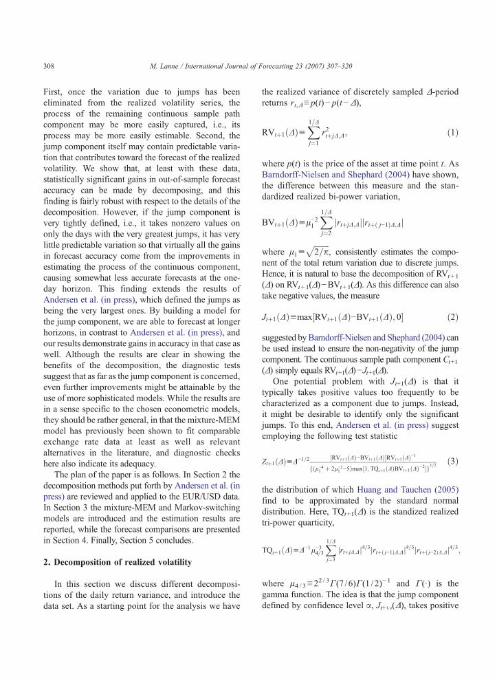
Fig. 1. The realized variance, bi-power variation an

instead of using the values of BVt+1(Δ) and TQt+1(Δ)defined above, we use the corresponding measures basedon staggered returns,

BV1;tþ1ðDÞul−21 ð1−2DÞ−1X1=D

j¼3

jrtþjD;Dj

� jrtþð j−2ÞD;Djand

TQ1;tþ1ðDÞuD−1l−34=3ð1−4DÞ−1X1=D

j¼5

jrtþjD;Dj4=3

� jrtþð j−2ÞD;Dj4=3jrtþð j−4ÞD;Dj4=3

in the empirical analysis, to mitigate the effects ofmicrostructure noise. Otherwise the statistic in Eq. (3)tends to find too few jumps, as pointed out by Huang andTauchen (2005).

The daily series of the realized volatility, continuoussample path and jump components are computed from

d jump component of the EUR/USD returns.

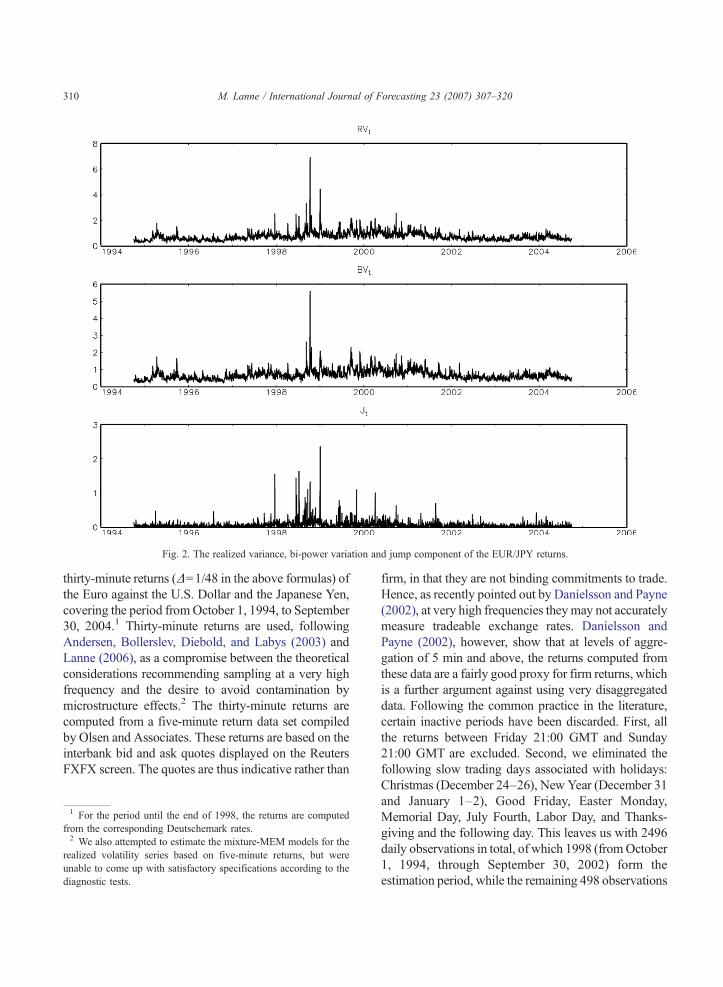
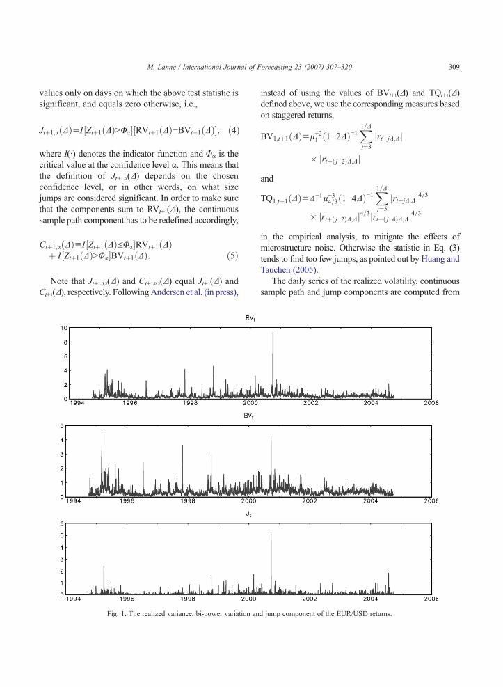
Fig. 2. The realized variance, bi-power variation and jump component of the EUR/JPY returns.


thirty-minute returns (Δ=1/48 in the above formulas) ofthe Euro against the U.S. Dollar and the Japanese Yen,covering the period fromOctober 1, 1994, to September30, 2004.1 Thirty-minute returns are used, followingAndersen, Bollerslev, Diebold, and Labys (2003) andLanne (2006), as a compromise between the theoreticalconsiderations recommending sampling at a very highfrequency and the desire to avoid contamination bymicrostructure effects.2 The thirty-minute returns arecomputed from a five-minute return data set compiledby Olsen and Associates. These returns are based on theinterbank bid and ask quotes displayed on the ReutersFXFX screen. The quotes are thus indicative rather than

1 For the period until the end of 1998, the returns are computedfrom the corresponding Deutschemark rates.2 We also attempted to estimate the mixture-MEM models for the

realized volatility series based on five-minute returns, but wereunable to come up with satisfactory specifications according to thediagnostic tests.

firm, in that they are not binding commitments to trade.Hence, as recently pointed out by Daníelsson and Payne(2002), at very high frequencies theymay not accuratelymeasure tradeable exchange rates. Daníelsson andPayne (2002), however, show that at levels of aggre-gation of 5 min and above, the returns computed fromthese data are a fairly good proxy for firm returns, whichis a further argument against using very disaggregateddata. Following the common practice in the literature,certain inactive periods have been discarded. First, allthe returns between Friday 21:00 GMT and Sunday21:00 GMT are excluded. Second, we eliminated thefollowing slow trading days associated with holidays:Christmas (December 24–26), New Year (December 31and January 1–2), Good Friday, Easter Monday,Memorial Day, July Fourth, Labor Day, and Thanks-giving and the following day. This leaves us with 2496daily observations in total, of which 1998 (fromOctober1, 1994, through September 30, 2002) form theestimation period, while the remaining 498 observations


(fromOctober 1, 2002, through September 30, 2004) areleft for the forecast evaluation.

The realized variance, bi-power variation and thejump component Jt+1(Δ) are depicted in Figs. 1 and 2.The maximum of all the series involving the U.S. Dollaroccurred on September 22, 2000. On that day, theEuropeanCentral Bank, the Federal Reserve, theBank ofJapan, the Bank of England and the Bank of Canada allbought euros in a coordinated intervention, presumablycausing the abrupt increase in volatility. An exceptionallyturbulent period for the EUR/YEN rate which is clearlyvisible in the plots, took place in the fall of 1998; forfurther discussion on the reasons for the excessivefluctuations of the Yen against the Deutschemark, see forinstance the annual report of the Bundesbank, 1998.

As the bottom panels of the figures show, the jumpcomponent defined in Eq. (2) takes a positive value onalmost every day, which is very different from the

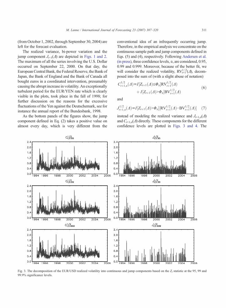
Fig. 3. The decomposition of the EUR/USD realized volatility into continu99.9% significance levels.

conventional idea of an infrequently occurring jump.Therefore, in the empirical analysis we concentrate on thecontinuous sample path and jump components defined inEqs. (5) and (4), respectively. Following Andersen et al.(in press), three confidence levels,α, are considered, 0.95,0.99 and 0.999. Moreover, because of the better fit, wewill consider the realized volatility, RVt+1

1 /2(Δ), decom-posed into the sum of (with a slight abuse of notation)

C1=2tþ1;aðDÞuI ½Ztþ1ðDÞVUa�RV1=2

tþ1ðDÞþ I ½Ztþ1ðDÞNUa�BV1=2

tþ1ðDÞð6Þ

and

J 1=2tþ1;aðDÞuI ½Ztþ1ðDÞNUa�½RV1=2tþ1ðDÞ−BV1=2

tþ1ðDÞ� ð7Þinstead of modeling the realized variance and Jt+1,α(Δ)andCt+1,α(Δ) directly. These components for the differentconfidence levels are plotted in Figs. 3 and 4. The

ous and jump components based on the Zt statistic at the 95, 99 and

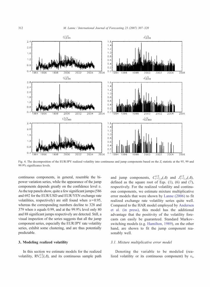
Fig. 4. The decomposition of the EUR/JPY realized volatility into continuous and jump components based on the Zt statistic at the 95, 99 and99.9% significance levels.


continuous components, in general, resemble the bi-power variation series, while the appearance of the jumpcomponents depends greatly on the confidence level α.As the top panels show, quite a few significant jumps (586and 692 for the EUR/USD and EUR/YEN exchange ratevolatilities, respectively) are still found when α=0.95,whereas the corresponding numbers decline to 328 and379 when α equals 0.99, and at the 99.9% level only 80and 88 significant jumps respectively are detected. Still, avisual inspection of the series suggests that all the jumpcomponent series, especially the EUR/JPY rate volatilityseries, exhibit some clustering, and are thus potentiallypredictable.

3. Modeling realized volatility

In this section we estimate models for the realizedvolatility, RVt+1

1/2(Δ), and its continuous sample path

and jump components, Ct+1,α1/2 (Δ) and Jt+1,α

1/2 (Δ),defined as the square root of Eqs. (1), (6) and (7),respectively. For the realized volatility and continu-ous components, we estimate mixture multiplicativeerror models that were shown by Lanne (2006) to fitrealized exchange rate volatility series quite well.Compared to the HAR model employed by Andersenet al. (in press), this model has the additionaladvantage that the positivity of the volatility fore-casts can easily be guaranteed. Standard Markov-switching models (e.g. Hamilton, 1989), on the otherhand, are shown to fit the jump component rea-sonably well.

3.1. Mixture multiplicative error model

Denoting the variable to be modeled (rea-lized volatility or its continuous component) by υt,

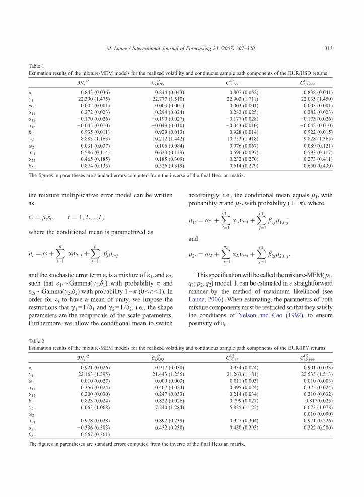
Table 1Estimation results of the mixture-MEM models for the realized volatility and continuous sample path components of the EUR/USD returns

RVt1/2 Ct,0.95

1/2 Ct,0.991/2 Ct,0.999

1/2

π 0.843 (0.036) 0.844 (0.043) 0.807 (0.052) 0.838 (0.041)γ1 22.390 (1.475) 22.777 (1.510) 22.903 (1.711) 22.035 (1.450)ω1 0.002 (0.001) 0.003 (0.001) 0.003 (0.001) 0.003 (0.001)α11 0.272 (0.023) 0.294 (0.024) 0.282 (0.025) 0.282 (0.023)α12 −0.170 (0.026) −0.190 (0.027) −0.177 (0.028) −0.173 (0.026)α16 −0.045 (0.010) −0.043 (0.010) −0.043 (0.010) −0.042 (0.010)β11 0.935 (0.011) 0.929 (0.013) 0.928 (0.014) 0.922 (0.015)γ2 8.883 (1.163) 10.212 (1.442) 10.753 (1.418) 9.828 (1.365)ω2 0.031 (0.037) 0.106 (0.084) 0.076 (0.067) 0.089 (0.121)α21 0.586 (0.114) 0.623 (0.113) 0.596 (0.097) 0.593 (0.117)α22 −0.465 (0.185) −0.185 (0.309) −0.232 (0.270) −0.273 (0.411)β21 0.874 (0.135) 0.526 (0.319) 0.614 (0.279) 0.650 (0.430)

The figures in parentheses are standard errors computed from the inverse of the final Hessian matrix.


the mixture multiplicative error model can be writtenas

tt ¼ ltet; t ¼ 1; 2; N T ;

where the conditional mean is parametrized as

lt ¼ xþXq

i¼1

aitt−i þXp

j¼1

bjlt−j

and the stochastic error term εt is a mixture of ε1t and ε2tsuch that ε1t∼Gamma(γ1,δ1) with probability π andε2t∼Gamma(γ2,δ2) with probability 1−π (0bπb1). Inorder for εt to have a mean of unity, we impose therestrictions that γ1=1 /δ1 and γ2=1/δ2, i.e., the shapeparameters are the reciprocals of the scale parameters.Furthermore, we allow the conditional mean to switch

Table 2Estimation results of the mixture-MEM models for the realized volatility a

RVt1/2 Ct,0.95

1/2

π 0.921 (0.026) 0.917 (0.030)γ1 22.163 (1.395) 21.443 (1.255)ω1 0.010 (0.027) 0.009 (0.003)α11 0.356 (0.024) 0.407 (0.024)α12 −0.200 (0.030) −0.247 (0.033)β11 0.823 (0.024) 0.822 (0.026)γ2 6.063 (1.068) 7.240 (1.284)ω2

α21 0.978 (0.028) 0.892 (0.239)α22 −0.336 (0.583) 0.452 (0.230)β21 0.567 (0.361)

The figures in parentheses are standard errors computed from the inverse o

accordingly, i.e., the conditional mean equals μ1t withprobability π and μ2t with probability (1−π), where

l1t ¼ x1 þXq1

i¼1

a1itt−i þXp1

j¼1

b1jl1;t−j

and

l2t ¼ x2 þXq2

i¼1

a2itt−i þXp2

j¼1

b2jl2;t−j:

This specificationwill be called themixture-MEM( p1,q1; p2, q2) model. It can be estimated in a straightforwardmanner by the method of maximum likelihood (seeLanne, 2006). When estimating, the parameters of bothmixture componentsmust be restricted so that they satisfythe conditions of Nelson and Cao (1992), to ensurepositivity of υt.

nd continuous sample path components of the EUR/JPY returns

Ct,0.991/2 Ct,0.999

1/2

0.934 (0.024) 0.901 (0.033)21.263 (1.181) 22.535 (1.513)0.011 (0.003) 0.010 (0.003)0.395 (0.024) 0.375 (0.024)

−0.214 (0.034) −0.210 (0.032)0.799 (0.027) 0.817(0.025)5.825 (1.125) 6.673 (1.078)

0.010 (0.090)0.927 (0.304) 0.971 (0.226)0.450 (0.293) 0.322 (0.200)

f the final Hessian matrix.


The estimation results are presented in Tables 1and 2. Based on the diagnostic checking, the mixture-MEM(1,6; 1,2) models were selected for all the EUR/USD rate return volatility series. Presumably the sixthlag is required for modeling some kind of weeklyseasonality in the series. The coefficients of the lagsbetween 2 and 6 of the first mixture component turnedout to be insignificant, so they are restricted to zero. Theerror distributions of the mixture components aredistinctly different, but the differences are similar acrossthe series. Plots of the error distributions (not shown)indicate that most of the time the errors come from adistribution relatively tightly concentrated around unity,whereas somewhat less than 20% of the time the errorsare generated from a right-skewed distribution with

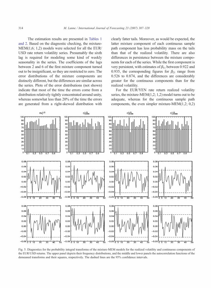
Fig. 5. Diagnostics for the probability integral transforms of the mixture-Mthe EUR/USD returns. The upper panel depicts their frequency distributionsdemeaned transforms and their squares, respectively. The dashed lines are

clearly fatter tails. Moreover, as would be expected, thelatter mixture component of each continuous samplepath component has less probability mass on the tailsthan that of the realized volatility. There are alsodifferences in persistence between the mixture compo-nents for each of the series. While the first component isvery persistent, with estimates of β11 between 0.922 and0.935, the corresponding figures for β21 range from0.526 to 0.874, and the differences are considerablygreater for the continuous components than for therealized volatility.

For the EUR/YEN rate return realized volatilityseries, the mixture-MEM(1,2; 1,2) model turns out to beadequate, whereas for the continuous sample pathcomponents, the even simpler mixture-MEM(1,2; 0,2)

EM models for the realized volatility and continuous components of, and the middle and lower panels the autocorrelation functions of thethe 95% confidence intervals.


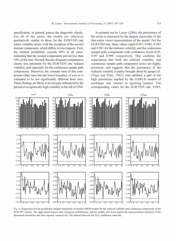
specification, in general, passes the diagnostic checks.For all of the series, the results are otherwisequalitatively similar to those for the EUR/USD ratereturn volatility series, with the exception of the secondmixture component, which differs in two respects. First,the mixture probability exceeds 90% in all cases,indicating that the second components prevail less than10% of the time. Second, this less frequent component isclearly less persistent for the EUR/YEN rate realizedvolatility, and especially for the continuous sample pathcomponents. Moreover, the constant term of this com-ponent either runs into the lower boundary of zero or isestimated to be not significantly different from zero.These findings are likely to be strongly influenced by theperiod of exceptionally high volatility in the fall of 1998.

Fig. 6. Diagnostics for the probability integral transforms of mixture-MEMEUR/JPY returns. The upper panel depicts their frequency distributions, ademeaned transforms and their squares, respectively. The dashed lines are

As pointed out by Lanne (2006), the persistence ofthe series is measured by the largest eigenvalue of thefirst-order vector representation of the model. For theEUR/USD rate, these values equal 0.987, 0.982, 0.983and 0.981 for the realized volatility and the continuoussample path components with confidence levels 0.95,0.99 and 0.999, respectively. This confirms theexpectation that both the realized volatility andcontinuous sample path component series are highlypersistent, and suggests that the persistence of therealized volatility is partly brought about by jumps (cf.(Vlaar and Palm, 1993), who attribute a part of thehigh persistence implied by the GARCH models ofexchange rate returns to ignoring jumps). Thecorresponding values for the EUR/YEN rate, 0.983,

models for the realized volatility and continuous components of thend the middle and lower panels the autocorrelation functions of thethe 95% confidence intervals.

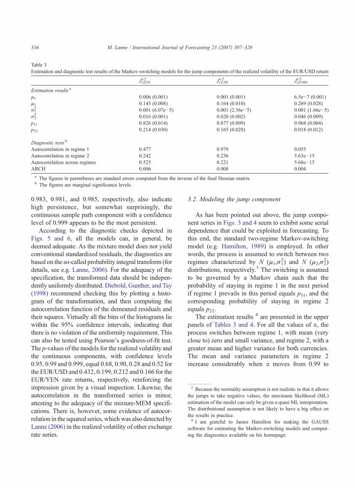
Table 3Estimation and diagnostic test results of the Markov-switching models for the jump components of the realized volatility of the EUR/USD return

Jt,0.951/2 Jt,0.99

1/2 Jt,0.9991/2

Estimation results a

μ1 0.006 (0.001) 0.001 (0.001) 6.5e−7 (0.001)μ2 0.145 (0.008) 0.164 (0.010) 0.269 (0.028)σ12 0.001 (6.07e−5) 0.001 (2.36e−5) 0.001 (1.66e−5)

σ22 0.016 (0.001) 0.020 (0.002) 0.046 (0.009)

p11 0.826 (0.014) 0.877 (0.009) 0.968 (0.004)p22 0.214 (0.030) 0.165 (0.028) 0.018 (0.012)

Diagnostic tests b

Autocorrelation in regime 1 0.477 0.979 0.055Autocorrelation in regime 2 0.242 0.236 5.63e−15Autocorrelation across regimes 0.525 0.221 5.68e−15ARCH 0.006 0.008 0.004

a The figures in parentheses are standard errors computed from the inverse of the final Hessian matrix.b The figures are marginal significance levels.

3 Because the normality assumption is not realistic in that it allowsthe jumps to take negative values, the maximum likelihood (ML)estimation of the model can only be given a quasi ML interpretation.The distributional assumption is not likely to have a big effect onthe results in practice.4 I am grateful to James Hamilton for making the GAUSS

software for estimating the Markov-switching models and comput-ing the diagnostics available on his homepage.


0.983, 0.981, and 0.985, respectively, also indicatehigh persistence, but somewhat surprisingly, thecontinuous sample path component with a confidencelevel of 0.999 appears to be the most persistent.

According to the diagnostic checks depicted inFigs. 5 and 6, all the models can, in general, bedeemed adequate. As the mixture model does not yieldconventional standardized residuals, the diagnostics arebased on the so-called probability integral transform (fordetails, see e.g. Lanne, 2006). For the adequacy of thespecification, the transformed data should be indepen-dently uniformly distributed. Diebold, Gunther, and Tay(1998) recommend checking this by plotting a histo-gram of the transformation, and then computing theautocorrelation function of the demeaned residuals andtheir squares. Virtually all the bins of the histograms liewithin the 95% confidence intervals, indicating thatthere is no violation of the uniformity requirement. Thiscan also be tested using Pearson's goodness-of-fit test.The p-values of the models for the realized volatility andthe continuous components, with confidence levels0.95, 0.99 and 0.999, equal 0.68, 0.90, 0.28 and 0.52 forthe EUR/USD and 0.432, 0.199, 0.212 and 0.166 for theEUR/YEN rate returns, respectively, reinforcing theimpression given by a visual inspection. Likewise, theautocorrelation in the transformed series is minor,attesting to the adequacy of the mixture-MEM specifi-cations. There is, however, some evidence of autocor-relation in the squared series, whichwas also detected byLanne (2006) in the realized volatility of other exchangerate series.

3.2. Modeling the jump component

As has been pointed out above, the jump compo-nent series in Figs. 3 and 4 seem to exhibit some serialdependence that could be exploited in forecasting. Tothis end, the standard two-regime Markov-switchingmodel (e.g. Hamilton, 1989) is employed. In otherwords, the process is assumed to switch between tworegimes characterized by N (μ1,σ1

2) and N (μ2,σ22)

distributions, respectively.3 The switching is assumedto be governed by a Markov chain such that theprobability of staying in regime 1 in the next periodif regime 1 prevails in this period equals p11, and thecorresponding probability of staying in regime 2equals p22.

The estimation results 4 are presented in the upperpanels of Tables 3 and 4. For all the values of α, theprocess switches between regime 1, with mean (veryclose to) zero and small variance, and regime 2, with agreater mean and higher variance for both currencies.The mean and variance parameters in regime 2increase considerably when α moves from 0.99 to

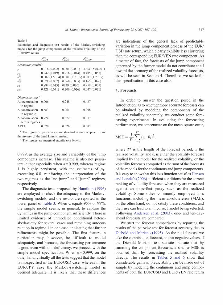
Table 4Estimation and diagnostic test results of the Markov-switchingmodels for the jump components of the realized volatility of theEUR/JPY return

Jt,0.951/2 Jt,0.99

1/2 Jt,0.9991/2

Estimation results a

μ1 0.018 (0.002) 0.001 (0.001) 3.66e−5 (0.001)μ2 0.242 (0.019) 0.216 (0.014) 0.405 (0.057)σ12 0.002 (1.5e−4) 0.001 (2.7e−5) 0.001 (1.7e−5)

σ22 0.071 (0.007) 0.060 (0.005) 0.165 (0.026)

p11 0.884 (0.013) 0839 (0.010) 0.958 (0.005)p22 0.321 (0.041) 0.206 (0.026) 0.047 (0.031)

Diagnostic tests b

Autocorrelationin regime 1

0.006 0.248 0.487

Autocorrelationin regime 2

0.683 0.261 0.098

Autocorrelationacross regimes

0.774 0.372 0.317

ARCH 0.070 0.026 0.003a The figures in parentheses are standard errors computed from

the inverse of the final Hessian matrix.b The figures are marginal significance levels.


0.999, as the average size and variability of the jumpcomponents increase. This regime is also not persis-tent, either especially when α=0.999, whereas regime1 is highly persistent, with the estimates of p11exceeding 0.8, reinforcing the interpretation of thetwo regimes as the “no jump” and “jump” regimes,respectively.

The diagnostic tests proposed by Hamilton (1996)are employed to check the adequacy of the Markov-switching models, and the results are reported in thelower panel of Table 3. When α equals 95% or 99%,the simple model seems, in general, to capture thedynamics in the jump component sufficiently. There islimited evidence of unmodeled conditional hetero-skedasticity for several cases and remaining autocor-relation in regime 1 in one case, indicating that furtherrefinements might be possible. The first feature inparticular may, however, be difficult to modeladequately, and because, the forecasting performanceis good even with this deficiency, we proceed with thesimple model specification. When α=0.999, on theother hand, virtually all the tests suggest that the modelis misspecified in the EUR/USD case, whereas in theEUR/JPY case the Markov-switching model isdeemed adequate. It is likely that these differences

are indications of the general lack of predictablevariation in the jump component process of the EUR/USD rate return, which clearly exhibits less clusteringthan the corresponding EUR/YEN rate component. Asa matter of fact, the forecasts of the jump componentgenerated by the former model do not contribute at alltoward the accuracy of the realized volatility forecasts,as will be seen in Section 4. Therefore, we settle forthis specification in this case also.

4. Forecasts

In order to answer the question posed in theIntroduction, as to whether more accurate forecasts canbe obtained by modeling the components of therealized volatility separately, we conduct some fore-casting experiments. In evaluating the forecastingperformance, we concentrate on the mean square error,

MSE ¼ 1T ⁎

XT⁎

t¼1

ðtt−t t̂Þ2;

where T⁎ is the length of the forecast period, υt therealized volatility, and υ̂t is either the volatility forecastimplied by the model for the realized volatility, or thevolatility forecasts computed as the sum of the forecastsof themodels for the continuous and jump components.It is easy to show that this loss function satisfies Hansenand Lunde's (2006) sufficient conditions for the correctranking of volatility forecasts when they are measuredagainst an imperfect proxy such as the realizedvolatility. Some other commonly employed lossfunctions, including the mean absolute error (MAE),on the other hand, do not satisfy these conditions, andtheir use can lead to an incorrect model being selected.Following Andersen et al. (2003), one- and ten-day-ahead forecasts are compared.

We start the forecast comparisons by reporting theresults of the pairwise test for forecast accuracy due toDiebold and Mariano (1995). As the null forecast wetake the combination forecast, so that negative values ofthe Diebold–Mariano test statistic indicate that bysumming the component forecasts, a smaller MSE isobtained than by forecasting the realized volatilitydirectly. The results in Tables 5 and 6 show thatconsiderable gains in predictability can be made out ofsample by modeling the continuous and jump compo-nents of both the EUR/USD and EUR/YEN rate return

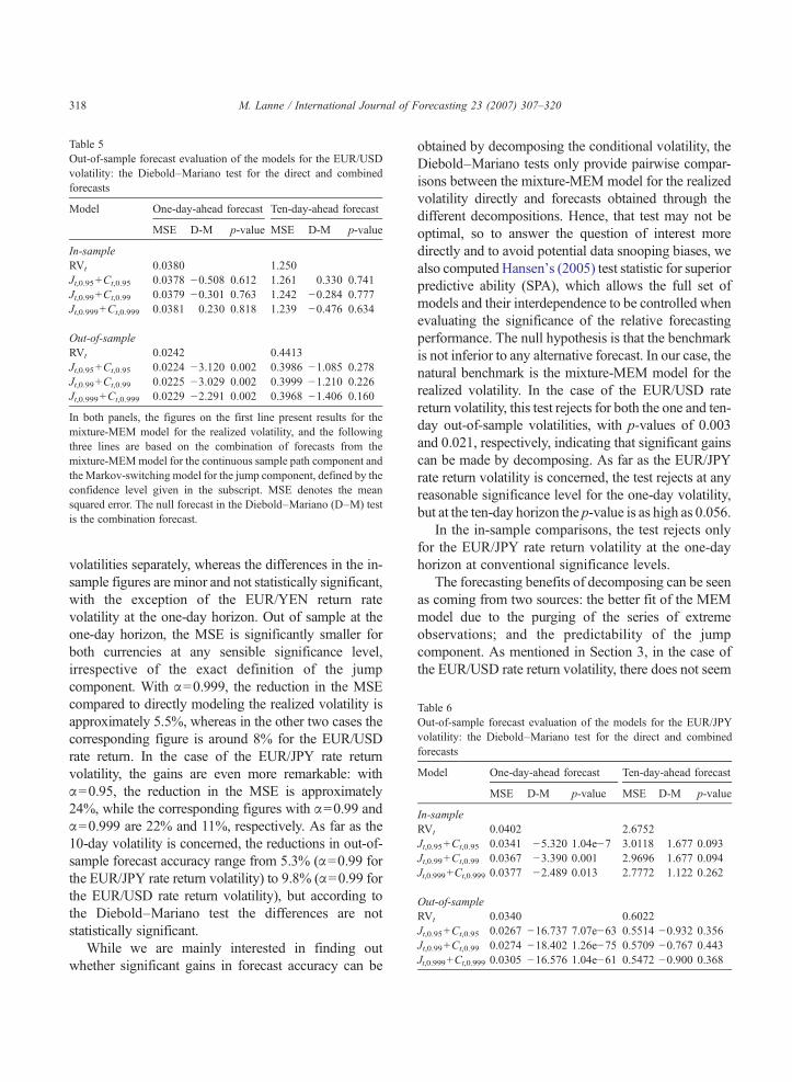
Table 5Out-of-sample forecast evaluation of the models for the EUR/USDvolatility: the Diebold–Mariano test for the direct and combinedforecasts

Model One-day-ahead forecast Ten-day-ahead forecast

MSE D-M p-value MSE D-M p-value

In-sampleRVt 0.0380 1.250Jt,0.95+Ct,0.95 0.0378 −0.508 0.612 1.261 0.330 0.741Jt,0.99+Ct,0.99 0.0379 −0.301 0.763 1.242 −0.284 0.777Jt,0.999+Ct,0.999 0.0381 0.230 0.818 1.239 −0.476 0.634

Out-of-sampleRVt 0.0242 0.4413Jt,0.95+Ct,0.95 0.0224 −3.120 0.002 0.3986 −1.085 0.278Jt,0.99+Ct,0.99 0.0225 −3.029 0.002 0.3999 −1.210 0.226Jt,0.999+Ct,0.999 0.0229 −2.291 0.002 0.3968 −1.406 0.160

In both panels, the figures on the first line present results for themixture-MEM model for the realized volatility, and the followingthree lines are based on the combination of forecasts from themixture-MEMmodel for the continuous sample path component andtheMarkov-switching model for the jump component, defined by theconfidence level given in the subscript. MSE denotes the meansquared error. The null forecast in the Diebold–Mariano (D–M) tesis the combination forecast.


t

able 6ut-of-sample forecast evaluation of the models for the EUR/JPYolatility: the Diebold–Mariano test for the direct and combinedorecasts

odel One-day-ahead forecast Ten-day-ahead forecast

MSE D-M p-value MSE D-M p-value

n-sampleVt 0.0402 2.6752

t,0.95+Ct,0.95 0.0341 −5.320 1.04e−7 3.0118 1.677 0.093

t,0.99+Ct,0.99 0.0367 −3.390 0.001 2.9696 1.677 0.094

t,0.999+Ct,0.999 0.0377 −2.489 0.013 2.7772 1.122 0.262

ut-of-sampleVt 0.0340 0.6022

t,0.95+Ct,0.95 0.0267 −16.737 7.07e−63 0.5514 −0.932 0.356

t,0.99+Ct,0.99 0.0274 −18.402 1.26e−75 0.5709 −0.767 0.443

t,0.999+Ct,0.999 0.0305 −16.576 1.04e−61 0.5472 −0.900 0.368

volatilities separately, whereas the differences in the in-sample figures are minor and not statistically significant,with the exception of the EUR/YEN return ratevolatility at the one-day horizon. Out of sample at theone-day horizon, the MSE is significantly smaller forboth currencies at any sensible significance level,irrespective of the exact definition of the jumpcomponent. With α=0.999, the reduction in the MSEcompared to directly modeling the realized volatility isapproximately 5.5%, whereas in the other two cases thecorresponding figure is around 8% for the EUR/USDrate return. In the case of the EUR/JPY rate returnvolatility, the gains are even more remarkable: withα=0.95, the reduction in the MSE is approximately24%, while the corresponding figures with α=0.99 andα=0.999 are 22% and 11%, respectively. As far as the10-day volatility is concerned, the reductions in out-of-sample forecast accuracy range from 5.3% (α=0.99 forthe EUR/JPY rate return volatility) to 9.8% (α=0.99 forthe EUR/USD rate return volatility), but according tothe Diebold–Mariano test the differences are notstatistically significant.

While we are mainly interested in finding outwhether significant gains in forecast accuracy can be

obtained by decomposing the conditional volatility, theDiebold–Mariano tests only provide pairwise compar-isons between the mixture-MEM model for the realizedvolatility directly and forecasts obtained through thedifferent decompositions. Hence, that test may not beoptimal, so to answer the question of interest moredirectly and to avoid potential data snooping biases, wealso computed Hansen's (2005) test statistic for superiorpredictive ability (SPA), which allows the full set ofmodels and their interdependence to be controlled whenevaluating the significance of the relative forecastingperformance. The null hypothesis is that the benchmarkis not inferior to any alternative forecast. In our case, thenatural benchmark is the mixture-MEM model for therealized volatility. In the case of the EUR/USD ratereturn volatility, this test rejects for both the one and ten-day out-of-sample volatilities, with p-values of 0.003and 0.021, respectively, indicating that significant gainscan be made by decomposing. As far as the EUR/JPYrate return volatility is concerned, the test rejects at anyreasonable significance level for the one-day volatility,but at the ten-day horizon the p-value is as high as 0.056.

In the in-sample comparisons, the test rejects onlyfor the EUR/JPY rate return volatility at the one-dayhorizon at conventional significance levels.

The forecasting benefits of decomposing can be seenas coming from two sources: the better fit of the MEMmodel due to the purging of the series of extremeobservations; and the predictability of the jumpcomponent. As mentioned in Section 3, in the case ofthe EUR/USD rate return volatility, there does not seem

TOvf

M

IRJJJ

ORJJJ


to be much predictable variation in the jump componentwhen only the greatest jumps are included (α=0.999),so that in this case the benefits come almost exclusivelyfrom the first factor. Thiswas reconfirmed by computingtheMSEs of the forecasts of the realized volatility basedonly on the continuous component. In the α=0.999 casethe figures were virtually unchanged, while in the othercases dismissing the jump component led to aconsiderable loss in forecast accuracy. In the case ofthe EUR/JPY rate return volatility, on the other hand, thejump component is predictable for all three values of α,albeit for this series as well the forecast accuracy clearlydeteriorates at the one-day horizon as α increases. Forthe ten-day volatility, the differences in predictiveaccuracy between the different values of α are minor.As a general conclusion, it could be said that, at leastwhen MEM and Markov-switching models are used, itis of less importance how the decomposition is done.This is probably due to the flexibility of the models infitting series with somewhat different properties, whichwas also indicated by the favorable diagnostic testresults.

5. Conclusion

Being EUR/USD and EUR/JPYexchange rate data ithas been shown that by decomposing the realizedvolatility into its jump and continuous sample pathcomponents, considerable gains in out-of-sample fore-cast accuracy can be obtained. Moreover, this findingseems to be relatively independent of the details of thedecomposition in the range typically considered. Hence,we have been able to answer the question posed byAndersen et al. (in press) of whether separately modelingand forecasting the two components is beneficial in theaffirmative. However, further work along these lines iscalled for, as our results may be specific to the particulardata sets andmodels. In particular, it would be interestingto see whether similar results were obtained with stockand bond market data. Although diagnostic tests suggestthat the chosen specification is adequate, comparablegains might not be possible when other commonly usedmodels are employed. The results of Andersen et al. (inpress) indicate that gains could be made by forecastingwith heterogenous autoregressive models specified forthe realized variance and its logarithm. This is likely to betrue for some other models as well. On the other hand,Lanne (2006) found that the mixture-MEM model

considered in this paper is superior to a large numberof rival models in forecasting realized exchange ratevolatility, suggesting that very large gains from decom-position are likely to be required to surpass that model.We leave this issue for future research.

Acknowledgements

I am grateful to participants at the ZeuthenWorkshop2006 in Copenhagen, the “Volatility Day”Workshop atStockholm School of Economics, and the joint financeresearch seminar at Helsinki School of Economics, aswell as to two anonymous referees for useful comments.The usual disclaimer applies. Financial support from theYrjö Jahnsson Foundation and Suomen Arvopaperi-markkinoiden Edistämissäätiö is gratefully acknowl-edged. Part of this research was done while the authorwas a JeanMonnet Fellow at the EconomicsDepartmentof the European University Institute.

References

Andersen, T. G., Bollerslev, T., & Diebold, F. X. (in press). Roughingit up: Including jump components in the measurement, modelingand forecasting of return volatility. Review of Economics andStatistics.

Andersen, T. G., Bollerslev, T., Diebold, F. X., & Labys, P. (2003).Modeling and forecasting realized volatility. Econometrica, 71,579−625.

Barndorff-Nielsen, O. E., & Shephard, N. (2004). Power andbipower variation with stochastic volatility and jumps. Journalof Financial Econometrics, 2, 1−37.

Corsi, F. (2003). A simple long memory model of realized volatility.Working paper : University of Southern Switzerland.

Daníelsson, J., & Payne, R. (2002). Real trading patterns and pricesin spot foreign exchange markets. Journal of InternationalMoney and Finance, 21, 203−222.

Diebold, F. X., Gunther, T., & Tay, A. S. (1998). Evaluating densityforecasts, with applications to financial risk management.International Economic Review, 39, 863−883.

Diebold, F. X., & Mariano, R. S. (1995). Comparing predictiveaccuracy. Journal of Business and Economic Statistics, 13,253−263.

Hamilton, J. D. (1989). A new approach to the economic analysis ofnonstationary time series and the business cycle. Econometrica,57, 357−384.

Hamilton, J. D. (1996). Specification testing in Markov-switchingtime-series models. Journal of Econometrics, 70, 127−157.

Hansen, P. R. (2005). A test for superior predictive ability. Journal ofBusiness and Economic Statistics, 23, 365−380.

Hansen, P. R., & Lunde, A. (2006). Consistent ranking of volatilitymodels. Journal of Econometrics, 131, 97−121.


Huang, X., & Tauchen, G. (2005). The relative contribution of jumpsto total price variance. Journal of Financial Econometrics, 3,456−499.

Lanne, M. (2006). A mixture multiplicative error model for realizedvolatility. Journal of Financial Econometrics, 4, 594−616.

Müller, U. A., Dacorogna, M. M., Davé, R. D., Olsen, R. B., Pictet,O. V., & von Weizsäcker, J. (1997). Volatilities of different timeresolutions—Analyzing the dynamics of market components.Journal of Empirical Finance, 4, 213−239.

Nelson, D. B., & Cao, C. Q. (1992). Inequality constraints in theunivariate GARCH model. Journal of Business and EconomicStatistics, 10, 229−235.

Vlaar, P. J. G., & Palm, F. C. (1993). The message in weeklyexchange rates in the European Monetary System: Meanreversion, conditional heteroskedasticity and jumps. Journal ofBusiness and Economic Statistics, 11, 351−360.

Markku Lanne is Professor of Economics at the University ofHelsinki, Finland. He graduated from the University of Helsinki,and holds a PhD in Economics. His current research interests are inthe areas of financial and macroeconometrics.

forecasting realized exchange rate volatility by decomposition

Documents