forecasting of indian stock market index using … · forecasting of indian stock market index...
TRANSCRIPT
FORECASTING OF INDIAN STOCK MARKET INDEX USING ARTIFICIAL NEURAL NETWORK
Manna Majumder1 , MD Anwar Hussian2
ABSTRACT
This paper presents a computational approach for predicting the S&P CNX Nifty 50 Index. A neural network based
model has been used in predicting the direction of the movement of the closing value of the index. The model presented
in the paper also confirms that it can be used to predict price index value of the stock market. After studying the
various features of the network model, an optimal model is proposed for the purpose of forecasting. The model has used
the preprocessed data set of closing value of S&P CNX Nifty 50 Index. The data set encompassed the trading days
from 1st January, 2000 to 31st December, 2009. In the paper, the model has been validated across 4 years of the
trading days. Accuracy of the performance of the neural network is compared using various out of sample
performance measures. The highest performance of the network in terms of accuracy in predicting the direction of the
closing value of the index is reported at 89.65% and with an average accuracy of 69.72% over a period of 4 years.
Keywords: Artificial Neural Network, Feed forward network, SCP, NMSE
1 The author is a professional banker. Email : [email protected]
2 Professor, Department of Electronics and Communication Engineering, North East Regional Institute of Science and
Technology, Email: [email protected]
The authors happily acknowledge the opportunity and the support extended for the research by National Stock Exchange of India
Limited. They also thank the anonymous referees for their guidance and valuable comments through out the research period. The
views and comments presented in the paper are those of the authors and not of National Stock Exchange of India Limited.
Forecasting Of Indian Stock Market Index Using Artificial Neural Network.
2
1. INTRODUCTION
Recently forecasting stock market return is gaining more attention, maybe because of the fact that if the
direction of the market is successfully predicted the investors may be better guided. The profitability of
investing and trading in the stock market to a large extent depends on the predictability. If any system be
developed which can consistently predict the trends of the dynamic stock market, would make the owner
of the system wealthy. More over the predicted trends of the market will help the regulators of the market
in making corrective measures.
Another motivation for research in this field is that it possesses many theoretical and experimental
challenges. The most important of these is the Efficient Market Hypothesis (EMH); see Eugene Fama’s
(1970) “Efficient Capital Markets”. The hypothesis says that in an efficient market, stock market prices fully
reflect available information about the market and its constituents and thus any opportunity of earning
excess profit ceases to exist. So it is ascertain that no system is expected to outperform the market
predictably and consistently. Hence, modeling any market under the assumption of EMH is only possible
on the speculative, stochastic component not on the changes on the changes in value or other fundamental
factors (Pan Heping., 2004). Another related theory to EMH is the Random Walk Theory, which states that
all future prices do not follow any trend or pattern and are random departure from the previous prices.
There has been a lot of debate about the validity of the EMH and random walk theory. However
with the advent of computational and intelligent finance, and behavioral finance, economists have tried to
establish an opposite hypothesis which may be collectively called as the Inefficient Market Hypothesis
(IMH). IMH states that financial markets are at least not always efficient, the market is not always in a
random walk, and inefficiencies exists. (Pan Heping., 2003). The origins of disparity of assumptions of
EMH go back to the work of Mandelbrot (1960), when he studied the cotton prices in New York exchange.
In his studies on the cotton prices he found that the data did not fit the normal distribution but instead
produced symmetry from the point of view of scaling. The sequences of changes are independent of
scaling; curves of daily changes and the curves of monthly change matched perfectly. Mandelbrot
presented the fractals of the financial markets. Subsequently, with evolution in this field of research Pan
Heping in 2003 postulated the Swing Market Hypothesis (SMH) which states that market is sometimes
efficient and sometimes inefficient; and the tends to swing between these two modes intermittently. The
theory also proposes that the market movement can be decomposed into four types of components:
dynamical swings, physical cycles, abrupt momentums and random walks. (Pan Heping)
Moreover, many researchers claim that the stock market is a chaos system. Chaos is a non linear
deterministic system which only appears random because of its irregular fluctuations. These systems are
highly sensitive to the initial conditions of the systems. These systems are dynamic, a periodic, complicated
and are difficult to deal with normal analytical methods. The neural networks are effective in learning such
non linear chaotic systems because they make very few assumptions about the functional form of the
underlying dynamic dependencies and their initial conditions. This may eventually question the
traditional financial theory of efficient market.
Many researchers and practitioners have proposed many models using various fundamental, technical and
analytical techniques to give a more or less exact prediction. Fundamental analysis involves the in-depth
analysis of the changes of the stock prices in terms of exogenous macroeconomic variables. It assumes that
the share price of a stock depends on its intrinsic value and the expected return of the investors. But this
expected return is subjected to change as new information pertaining to the stock is available in the market
which in turn changes the share price. Moreover, the analysis of the economic factors is quite subjective as
Forecasting Of Indian Stock Market Index Using Artificial Neural Network.
3
the interpretation totally lays on the intellectuality of the analyst. Alternatively, technical analysis centers
on using price, volume, and open interest statistical charts to predict future stock movements. The premise
behind technical analysis is that all of the internal and external factors that affect a market at any given
point of time are already factored into that market’s price. (Louis. B. Mendelsohn, 2000).
Apart from these commonly used methods of prediction, some traditional time series forecasting tools are
also used for the same. In time series forecasting, the past data of the prediction variable is analyzed and
modeled to capture the patterns of the historic changes in the variable. These models are then used to
forecast the future prices.
There are mainly two approaches of time series modeling and forecasting: linear approach and the
nonlinear approach. Mostly used linear methods are moving average, exponential smoothing, time series
regression etc. One of the most common and popular linear method is the Autoregressive integrated
moving average (ARIMA) model (Box and Jenkins (1976)). It presumes linear model but is quite flexible as it
can represent different types of time series, i.e. Autoregressive (AR), moving average (MA) and combined
AR and MA (ARMA) series.
However, there is not much evidence that the stock market returns are perfectly linear for the very reason
that the residual variance between the predicted return and the actual is quite high. The existence of the
nonlinearity of the financial market is propounded by many researchers and financial analyst. (Abhyankar
et al., 1997). Some parametric nonlinear model such as Autoregressive Conditional Heteroskedasticity and
General Autoregressive Conditional Heteroskedasticity has been in use for financial forecasting. But most
of the non linear statistical techniques require that the non linear model must be specified before the
estimation of the parameters is done.
During last few years there has been much advancement in the application of neural network in stock
market indices forecasting with a hope that market patterns can be extracted. The novelty of the ANN lies
in their ability to discover nonlinear relationship in the input data set without a priori assumption of the
knowledge of relation between the input and the output. (Hagen et al., 1996). They independently learn the
relationship inherent in the variables. From statistical point of view neural networks are analogous to
nonparametric, nonlinear, regression model. So, neural network suits better than other models in
predicting the stock market returns.
A neural network is a massively parallel distributed processor made up of simple processing unit which
has a natural propensity for storing experiential knowledge and making it available for use. (Simon
Haykin, (1999). Neural networks have remarkable ability to derive meaning from complicated or imprecise
data. They are used to extract patterns and detect trends that are too complex to be noticed by either
humans or other computer techniques. From statistical inference neural networks are analogous to
nonparametric, nonlinear, regression model. However, the traditional statistical models have limitations in
understanding the relationship between the input and the output of the system because of the complex and
chaos nature of the system.
There are several distinguished features that propound the use of neural network as a preferred tool over
other traditional models of forecasting.
Neural networks are nonlinear in nature and where most of the natural real world systems are non linear
in nature, neural networks are preferred over the traditional linear models. This is because the linear
models generally fail to understand the data pattern and analyze when the underlying system is a non
linear one. However, some parametric nonlinear model such as Autoregressive Conditional
Heteroskedasticity (Engle, 1982) and General Autoregressive Conditional Heteroskedasticity have been in
use for financial forecasting. But most of the non linear statistical techniques require that the non linear
Forecasting Of Indian Stock Market Index Using Artificial Neural Network.
4
model must be specified before the estimation of the parameters is done and generally it happens that pre-
specified nonlinear models may fail to observe the critical features of the complex system under study.
Neural networks are data driven models. The novelty of the neural network lies in their ability to discover
nonlinear relationship in the input data set without a priori assumption of the knowledge of relation
between the input and the output (Hagen et al., 1996) The input variables are mapped to the output
variables by squashing or transforming by a special function known as activation function. They
independently learn the relationship inherent in the variables from a set of labeled training example and
therefore involves in modification of the network parameters.
Neural Networks have a built in capability to adapt the network parameters to the changes in the studied
system. A neural network trained to a particular input data set corresponding to a particular environment;
can be easily retrained to a new environment to predict at the same level of environment. Moreover, when
the system under study is non stationary and dynamic in nature, the neural network can change its
network parameters (synaptic weights) in real time.
So, neural network suits better than other models in predicting the stock market returns.
2. LITERATURE REVIEW
In the last two decades forecasting of stock returns has become an important field of research. In most of
the cases the researchers had attempted to establish a linear relationship between the input macroeconomic
variables and the stock returns. But with the discovery of nonlinearity in the stock market index returns (A.
Abhyankar et al. 1997), there has been a great shift in the focus of the researchers towards the nonlinear
prediction of the stock returns. Although, there after many literatures have come up in nonlinear statistical
modeling of the stock returns, most of them required that the nonlinear model be specified before the
estimation is done. But for the reason that the stock market return being noisy, uncertain, chaotic and
nonlinear in nature, ANN has evolved out to be better technique in capturing the structural relationship
between a stock’s performance and its determinant factors more accurately than many other statistical
techniques (Refenes et al., S.I. Wu et al., Schoeneburg, E.,)
In literature, different sets of input variables are used to predict stock returns. In fact, different input
variables are used to predict the same set of stock return data. Some researchers used input data from a
single time series where others considered the inclusion of heterogeneous market information and macro
economic variables. Some researchers even preprocessed these input data sets before feeding it to the ANN
for forecasting.
Chan., Wong.,and Lam., implemented a neural network model using the technical analysis variables for
listed companies in Shanghai Stock Market. In this paper performance of two learning algorithm and two
weight initialization methods are compared. The results reported that prediction of stock market is quite
possible with both the algorithm and initialization methods but the performance of the efficiency of the
back propagation can be increased by conjugate gradient learning and with multiple linear regression
weight initializations.
Other prominent literatures are that of Siekmann et al. (2001) who used fuzzy rules to split inputs into
increasing, stable, and decreasing trend variables. Siekmann et al. (2001) implemented a network structure
that contains the adaptable fuzzy parameters in the weights of the connections between the first and
second hidden layers.
Kim and Han (2000) used a genetic algorithm to transform continuous input values into discrete ones. The
genetic algorithm was used to reduce the complexity of the feature space.
Forecasting Of Indian Stock Market Index Using Artificial Neural Network.
5
Kishikawa and Tokinaga (2000) used a wavelet transform to extract the short-term feature of stock trends.
Kim and Han (2000) used neural network modified by Genetic Algorithm. Kim and Chun (1998) used
refined probabilistic NN (PNN) to predict a stock market index. Pantazopoulos et al. (1998) presented a
neurofuzzy approach for predicting the prices of IBM stock.
Chenoweth, Tim., Obradovic, Zoran., used specialized neural network as preprocessing component and a
decision rule base. The preprocessing component determine the most relevant features for stock market
prediction, remove the noise, and separate the remaining patterns into two disjoint sets. Next, the two
neural networks predict the market's rate of return, with one network trained to recognize positive and the
other negative returns.
Some work has also been reported in portfolio construction, for Roman, Jovina and Jameel, Akhtar in their
paper proposed a new methodology to aid in designing a portfolio of investment over multiple stock
markets. For that they used backpropagation and recurrent network and also the contextual market
information. They developed a determinant using the accuracy of prediction of the neural network and the
stock return of the previous year and used it to select the stock market among other markets.
In the work by Refenes et al, (1997), they compared the performance of backpropagation network and
regression models to predict the stock market returns. Desai, V. S. (1998), compared the performance of
linear regression with that of the neural network in forecasting the stock returns.
In many papers ARIMA model has been used as a benchmark model in order to compare the forecasting
accuracy of the ANN. Jung-Hua Wang; Jia-Yann Leu developed a prediction system of recurrent neural
network trained by using features extracted from ARIMA analysis. Then after differencing the raw data of
the TSEWSI series and then examining the autocorrelation and partial autocorrelation function plots, they
identified the series as a nonlinear version of ARIMA (1,2,1). Neural networks were trained by using
second difference data and were seen to give better predictions than otherwise trained by using raw data.
Jingtao Yao, Chew Lim Tan and Hean-Lee Poh developed a neural network that was used to predict the
stock index of Kuala Lumpur Stock Exchange. The used trading strategies to a paper profit were recorded
and were compared with that of the ARIMA model. The results showed that the performance of the neural
net was better than that of the ARIMA. It was also asserted that useful prediction can be made even
without the use of extensive data or knowledge.
Researchers have tested the accuracy of ANN in predicting the stock market index return of most
developed economies across the globe. Literatures are available for forecasting index returns of U.S
markets like NYSE [19], FTSE [4], DJIA [5], S&P500 [2, 6]. Few papers are also available in context to Asian
stock markets like Hang Seng Stock Exchange, Korea Stock Exchange Tokyo Stock Exchange and Taiwan
Stock Exchange.
Some literatures are also available in Indian context. Panda, C. and Narasimhan, V. used the artificial
neural network to forecast the daily returns of Bombay Stock Exchange (BSE) Sensitive Index (Sensex).
They compared the performance of the neural network with performances of random walk and linear
autoregressive models. They reported that neural network out-performs linear autoregressive and random
walk models by all performance measures in both in-sample and out-of-sample forecasting of daily BSE
Sensex returns.
In another paper, Dutta,G. et.al. studied the efficacy of ANN in modeling the Bombay Stock Exchange
(BSE) SENSEX weekly closing values. They developed two networks with inputs as the weekly closing
value, 52-week moving average of the weekly closing SENSEX values, 5-week moving average of the same,
Forecasting Of Indian Stock Market Index Using Artificial Neural Network.
6
and the 10-week Oscillator for the past 200 weeks for one neural net. And for the other network the inputs
are the weekly closing value, 52-week moving average of the weekly closing SENSEX values, 5-week
moving average of the same and the 5-week volatility for the past 200 weeks.
To assess the performance of the networks they used the neural networks to predict the weekly closing
SENSEX values for the two-year period beginning January 2002. The root mean square error (RMSE) and
mean absolute error (MAE) are chosen as indicators of performance of the networks. The proposed
network has been tested with stock data obtained from the Indian stock Market BSE Index. Bishnoi T. R., et
al has analyzed the behavior of daily and weekly returns of five Indian stock market indices for random
walk during April-1996 to June-2001. They have tested the indices for normality, autocorrelation using Q-
statistic & Dickey-Fuller test and analyzed variance ratio using homoscedastic and heteroscedastic test
estimates. The results support that Indian stock market indices do not follow random walk.
The previous studies have used various forecasting techniques in order to predict the stock market trends.
Some attempted to forecast the daily returns where others developed forecasting models to predict the rate
of returns of individual stocks. In many papers it was also found that researchers have attempted to
compare their results with other statistical tools. And these findings provide strong motivation for
modeling forecasting tools for stock market prediction.
The uniqueness of the research comes from the fact that the research employs a neural network based
forecasting approach on National Stock Exchange index (CNX S&P Nifty 50) Furthermore, as not much
work has been done on the forecasting of Indian stock market indices using neural network, this paper will
actually help to understand the microstructure of Indian market
3. DATA AND METHODOLOGY
The data employed in the study consists of daily closing prices of S&P CNX Nifty 50 Index. The data set
encompassed the trading days from 1st January, 2000 to 31st December, 2009. The data is collected from the
historical data available on the website of National Stock Market. The study makes an attempt to design a
simple neural network model where in most of the critical issues pertaining to performance of the neural
network will be addressed.
The performance of the neural network largely depends on the model of the Neural Network. Issues
critical to the neural network modeling like selection of input variables, data preprocessing technique,
network architecture design and performance measuring statistics, are considered carefully.
Selection of input variables:
Selection of input variable for the neural network model is a critical factor for the performance of the
neural network because it contains important information about the complex non linear structures of the
data. It also facilitates the neural network to understand the movements in the time series. The input
variables selected for this model are the lagged observation of the time series being forecasted, which in
this case is the closing prices of S&P CNX Nifty 50 Index. The criticality in selecting the input variables lies
in selecting the number of input variables and the lag between each. With less of lag between the inputs the
correlation between the lagged variable increases which may result in an over-fitting phenomenon. On the
other hand, with increase in the lag between each input variable the neural network may loose out
essential information of input variables, resulting in under-learning. To handle with this dilemma of over-
fitting or under-learning and select an optimal structure, we have considered various lagged structure
(multiple lag input variable with different lag between each) and test the performance of the neural
network on a trial and error basis.
Forecasting Of Indian Stock Market Index Using Artificial Neural Network.
7
b
n w Σ X
Y= f (wX+b)
Y ffff
In order to select the neural network model and for validating the performance of the network model, the
whole historical data set is divided into in-sample and out of sample data set. The in-sample data set is
used to construct the neural network model and for training the same. The out-of- sample data set is used
to evaluate how well the network performs in forecasting with the new data set, which was not used to
train and estimate the coefficients of the network. To study the performance of the network model across
the historical range of data, the neural network performance is tested at different historic periods.
Data Preprocessing
The performance and the reliability of a neural network model also to a large extent depend on the quality
of the data used. As neural networks are pattern recognizers, the data presented to it largely influences the
accuracy of the result. The data preprocessing of the input variable of the neural network model facilitates
de-trending of the data and highlight essential relationship, so as to facilitate proper network learning
process. Various preprocessing methods are considered and tested for an optimal result.
The closing prices of the index were scaled with linear scaling functions. The linear scaling function used
the maximum and the minimum values of the data series and scaled the series to an interval of [0, 1]. The
function used was:
)min()max(
)min(*
,
,
kk
knk
nkXX
XXX
−
−= (1)
Here in equation (1), kX is the data series of the all the closing price of the index and nkX , is the nth day’s
closing price of the index.
In order to improve the performance of the network a non linear scaling method is adopted. Before non
linear scaling the data series was scaled down at a rate of 50 in order to reduce the search space for finding
the optimal coefficient estimates. The network showed better results with a scaling factor of 50. Then a
logarithmic first differencing was used to preprocess the scaled down series of closing price of the index.
Logarithmic first difference takes the logarithmic value of the series and then taking the difference.
(2)
Here in equation (2), )1(, −nkX is the previous day’s (the day before nkX , ) value of closing price of the index.
Neural Network Architecture and Design:
A neural network is a massively parallel distributed processor made up of simple processing unit which
has a natural propensity for storing experiential knowledge and making it available for use. (Simon
Haykin, (1999). Neural networks has remarkable ability to derive meaning from complicated or imprecise
data, can be used to extract patterns and detect trends that are too complex to be noticed by either humans
or other computer techniques. A trained neural network can be thought of as an "expert" in the category of
information it has been given to analyze.
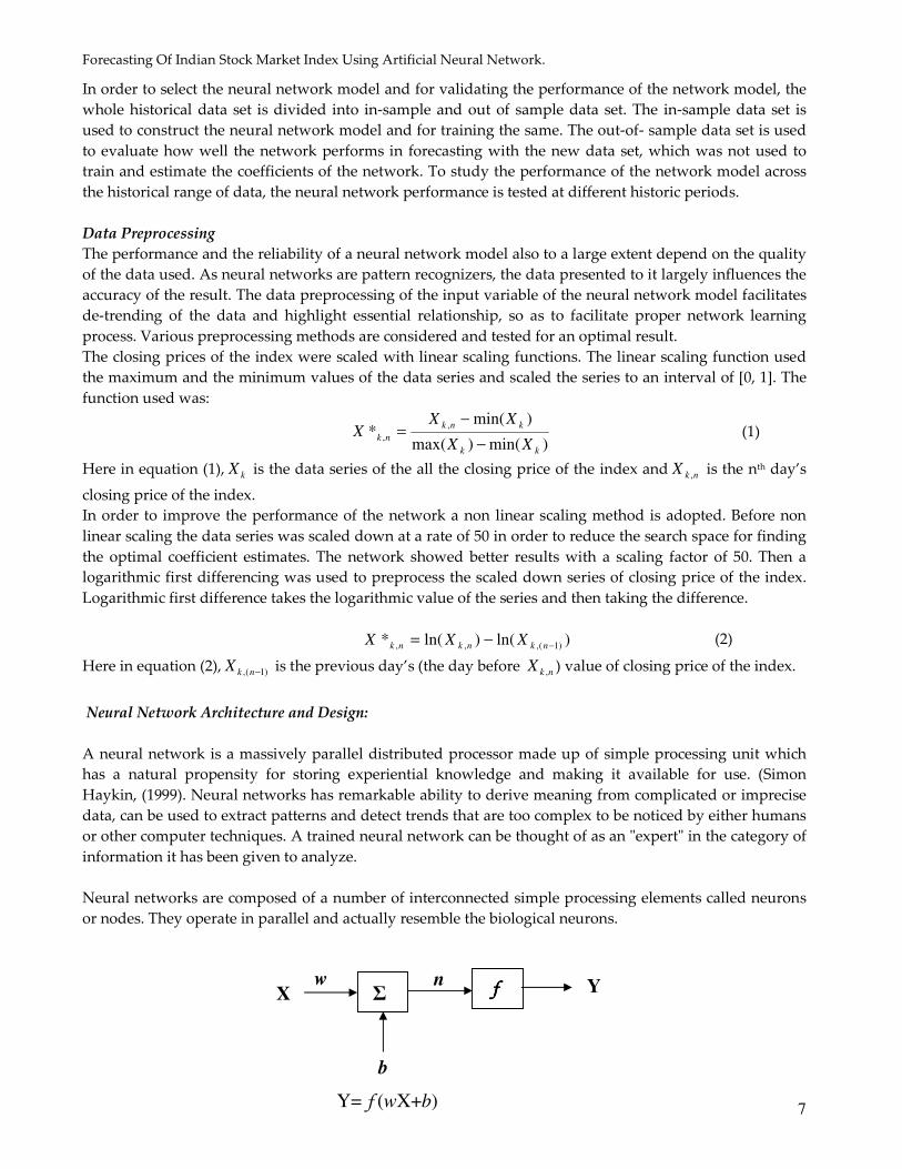
Neural networks are composed of a number of interconnected simple processing elements called neurons
or nodes. They operate in parallel and actually resemble the biological neurons.
)ln()ln(* )1(,,, −−= nknknk XXX
Forecasting Of Indian Stock Market Index Using Artificial Neural Network.
8
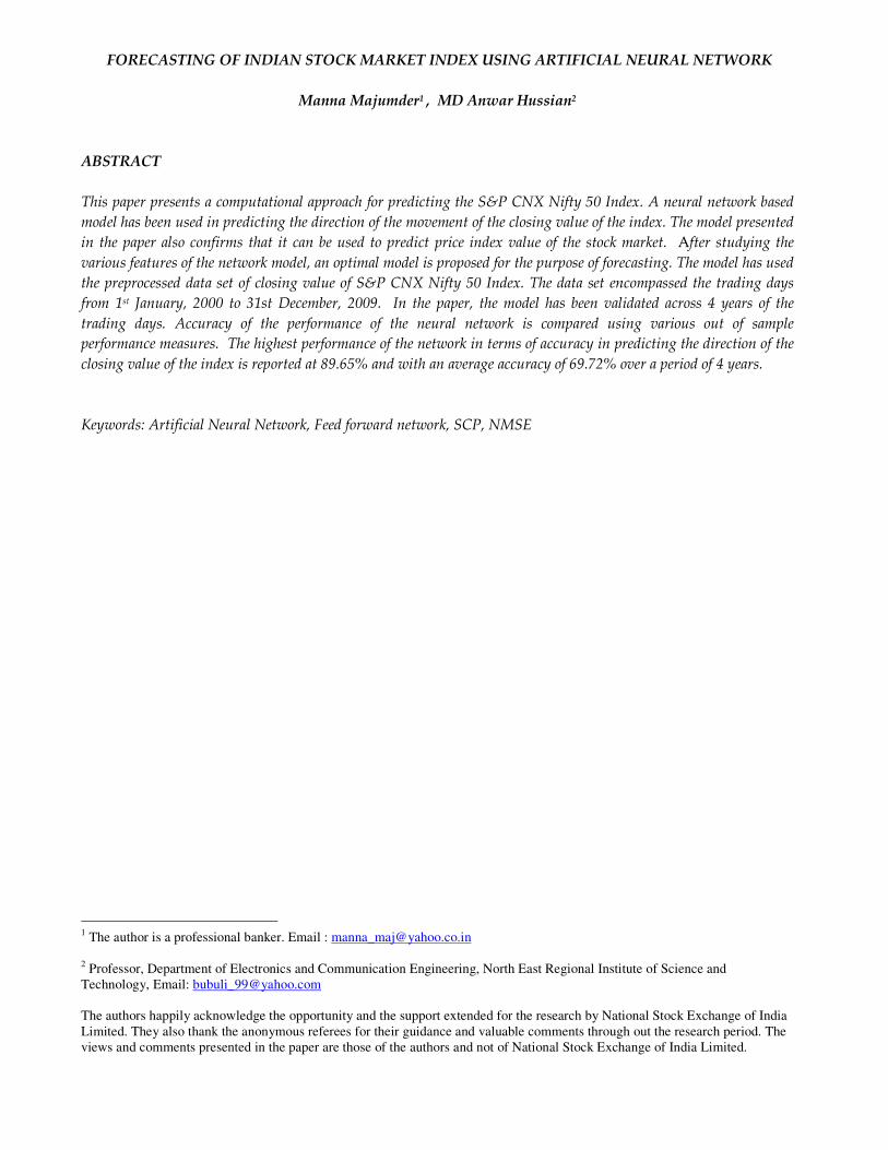
The neuron acts as a processing unit to transform the input to get an output. The neuron, like other linear
or polynomial approximation, relates a set of input variables {Xi}, i=1,……k, to set of one or more output
variables {Yi}, i=1,……k. But in case of neural network the only difference is that it does not require any
prior equation as in case of other approximation methods, rather the input variables are mapped to the
output set by squashing or transforming by a special function known as activation function. Each neuron
has a weight and a bias assigned to it. Each neuron receives an input signal, which transmits through a
connection that multiplies its strength by the scalar weight w, to form the product wX. A bias is added to
the weighted
input and is then passed through a transfer function to get the desired output. The weight w and the bias b
are the adjustable parameters of the neuron and are adjusted so that the neuron exhibits a desired
behavior.
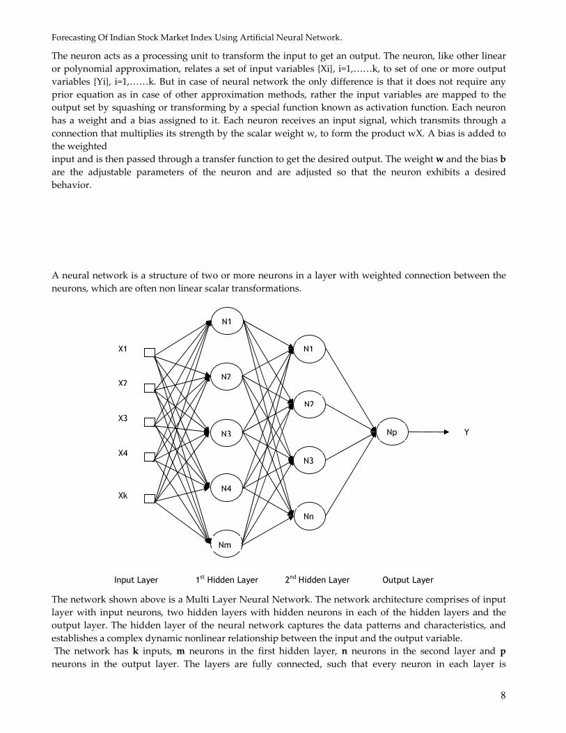
A neural network is a structure of two or more neurons in a layer with weighted connection between the
neurons, which are often non linear scalar transformations.
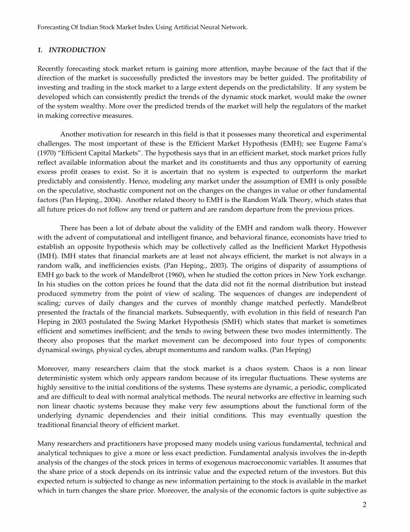
The network shown above is a Multi Layer Neural Network. The network architecture comprises of input
layer with input neurons, two hidden layers with hidden neurons in each of the hidden layers and the
output layer. The hidden layer of the neural network captures the data patterns and characteristics, and
establishes a complex dynamic nonlinear relationship between the input and the output variable.
The network has k inputs, m neurons in the first hidden layer, n neurons in the second layer and p
neurons in the output layer. The layers are fully connected, such that every neuron in each layer is
Np
N1
N2
N3
N4
Nm
N1
N2
N3
Nn
X1
X2
X3
X4
Xk
Y
Input Layer 1st Hidden Layer 2nd Hidden Layer Output Layer
Forecasting Of Indian Stock Market Index Using Artificial Neural Network.
9
connected to every neuron in the next layer. The output of one hidden layer is the input of the following
layer. Each neuron in the first hidden layer has k inputs. So there are kxm no of weighted input
connections to the layer. Similarly, the second hidden layer has mxn inputs. The output layer has n inputs
and p outputs. Selection of the hidden layers in the network and the no of the neurons in each of the layers
are fundamental to the structure of the neural network. The input and the output neurons can easily be
determined from the no of the input and the output variables used in the model as they are equal to the
input and the output variables.
The relationship between the input and the output of a neuron is established by the transfer function of the
layer. The transfer function is a step function or a sigmoid function which takes the weighted input n and
produces the output Y. Based on the performance of the network model transfer function are finalized for
the network model.
Network Training
After the neural network model is constructed, training of the neural network is the next essential step of
the forecasting model. Training of neural network is an iterative process of non linear optimization of the
parameters like weights and bias of the network. The result of the training process of the network depends
on the algorithm used for the purpose. In this paper backpropagation algorithm is used training. A
backpropagation network uses a supervised learning method for training.
In one complete cycle of the training process, a set of input data {X1, X2, X3…} is presented to the input
node. The corresponding target output Dp(n), is presented to the output node in order to show the
network what type of behavior is expected. The output signal is compared with the desired response or
target output and consequently an error signal is produced. In each step of iterative process, the error
signal activates a control mechanism which applies a sequence of corrective adjustments of the weights
and biases of the neuron. The corrective adjustments continue until the training data attains the desired
mapping to obtain the target output as closely as possible. After a number of iterations the neural network
is trained and the weights are saved. The test set of data is presented to the trained neural network to test
the performance of the neural network. The result is recorded to see how well the net is able to predict the
output using the adjusted weights of the network.
Two training algorithms, gradient descent adaptive back-propagation and gradient descent with
momentum and adaptive learning back-propagation are considered in our model.
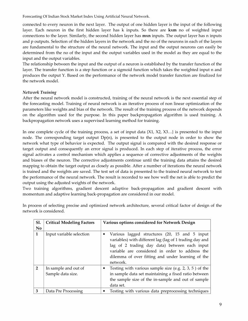
In process of selecting precise and optimized network architecture, several critical factor of design of the
network is considered.
Sl.
No
Critical Modeling Factors Various options considered for Network Design
1 Input variable selection • Various lagged structures (20, 15 and 5 input
variables) with different lag (lag of 1 trading day and
lag of 2 trading day data) between each input
variable are considered in order to address the
dilemma of over fitting and under learning of the
network.
2 In sample and out of
Sample data size.
• Testing with various sample size (e.g. 2, 3, 5 ) of the
in sample data set maintaining a fixed ratio between
the sample size of the in-sample and out of sample
data set.
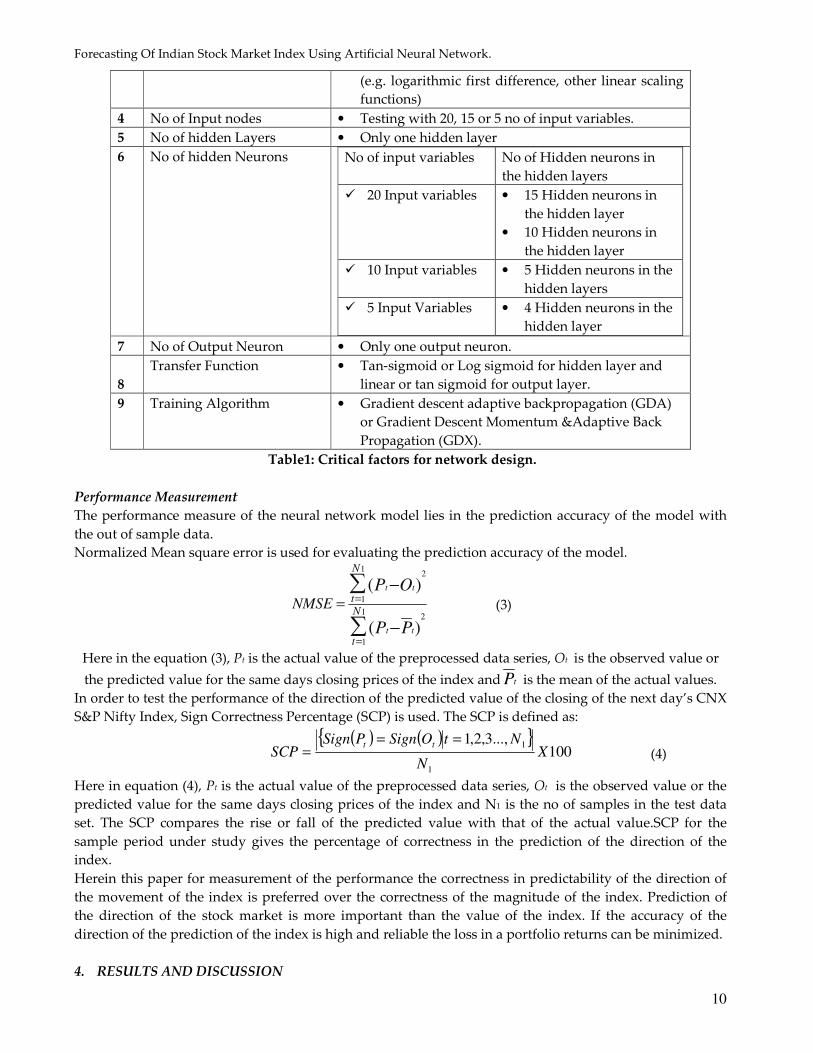
3 Data Pre Processing • Testing with various data preprocessing techniques
Forecasting Of Indian Stock Market Index Using Artificial Neural Network.
10
(e.g. logarithmic first difference, other linear scaling
functions)
4 No of Input nodes • Testing with 20, 15 or 5 no of input variables.
5 No of hidden Layers • Only one hidden layer
6 No of hidden Neurons No of input variables No of Hidden neurons in
the hidden layers
� 20 Input variables • 15 Hidden neurons in
the hidden layer
• 10 Hidden neurons in
the hidden layer
� 10 Input variables • 5 Hidden neurons in the
hidden layers
� 5 Input Variables • 4 Hidden neurons in the
hidden layer
7 No of Output Neuron • Only one output neuron.
8
Transfer Function • Tan-sigmoid or Log sigmoid for hidden layer and
linear or tan sigmoid for output layer.
9 Training Algorithm • Gradient descent adaptive backpropagation (GDA)
or Gradient Descent Momentum &Adaptive Back
Propagation (GDX).
Table1: Critical factors for network design.
Performance Measurement
The performance measure of the neural network model lies in the prediction accuracy of the model with
the out of sample data.
Normalized Mean square error is used for evaluating the prediction accuracy of the model.
∑
∑
=
=
−
−=
1
1
2
1
1
2
)(
)(
N
t
N
t
tt
tt
PP
OPNMSE (3)
Here in the equation (3), Pt is the actual value of the preprocessed data series, Ot is the observed value or
the predicted value for the same days closing prices of the index and tP is the mean of the actual values.
In order to test the performance of the direction of the predicted value of the closing of the next day’s CNX
S&P Nifty Index, Sign Correctness Percentage (SCP) is used. The SCP is defined as:
(4)
Here in equation (4), Pt is the actual value of the preprocessed data series, Ot is the observed value or the
predicted value for the same days closing prices of the index and N1 is the no of samples in the test data
set. The SCP compares the rise or fall of the predicted value with that of the actual value.SCP for the
sample period under study gives the percentage of correctness in the prediction of the direction of the
index.
Herein this paper for measurement of the performance the correctness in predictability of the direction of
the movement of the index is preferred over the correctness of the magnitude of the index. Prediction of
the direction of the stock market is more important than the value of the index. If the accuracy of the
direction of the prediction of the index is high and reliable the loss in a portfolio returns can be minimized.
4. RESULTS AND DISCUSSION
( ) ( ){ }100
...,3,2,1
1
1X
N
NtOSignPSignSCP
tt ===
Forecasting Of Indian Stock Market Index Using Artificial Neural Network.
11
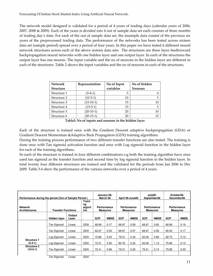
The network model designed is validated for a period of 4 years of trading days (calendar years of 2006,
2007, 2008 & 2009). Each of the years is divided into 4 out of sample data set each consists of three months
of trading day’s data. For each of the out of sample data set, the insample data consist of the previous six
years of the preprocessed trading data. The performance of the networks has been tested across sixteen
data set (sample period) spread over a period of four years. In this paper we have tested 6 different neural
network structures across each of the above sixteen data sets. The structures are three layer feedforward
backpropagation neural networks with one hidden layer and one output layer. In each of the structures the
output layer has one neuron. The input variable and the no of neurons in the hidden layer are different in
each of the structures. Table 2 shows the input variables and the no of neurons in each of the structures.
Network
Structure
Representation No of Input
variables
No of hidden
Neurons
Structure 1 (5-4-1) 5 4
Structure 2 (10-5-1) 10 5
Structure 3 (15-10-1) 15 10
Structure 4 (15-5-1) 15 5
Structure 5 (20-10-1) 20 10
Structure 6 (20-15-1) 20 15
Table2: No of inputs and neurons in the hidden layer
Each of the structure is trained once with the Gradient Descent adaptive backpropagation (GDA) or
Gradient Descent Momentum &Adaptive Back Propagation (GDX) training algorithms.
During the training process performance of two different transfer functions are also tested. The training is
done once with Tan sigmoid activation function and once with Log sigmoid function in the hidden layer
for each of the training algorithms.
So each of the structure is trained in four different combinations e.g both the training algorithm have once
used tan sigmoid as the transfer function and second time by log sigmoid function in the hidden layer. In
total twenty four different structures are trained and the validated for the periods from Jan 2006 to Dec
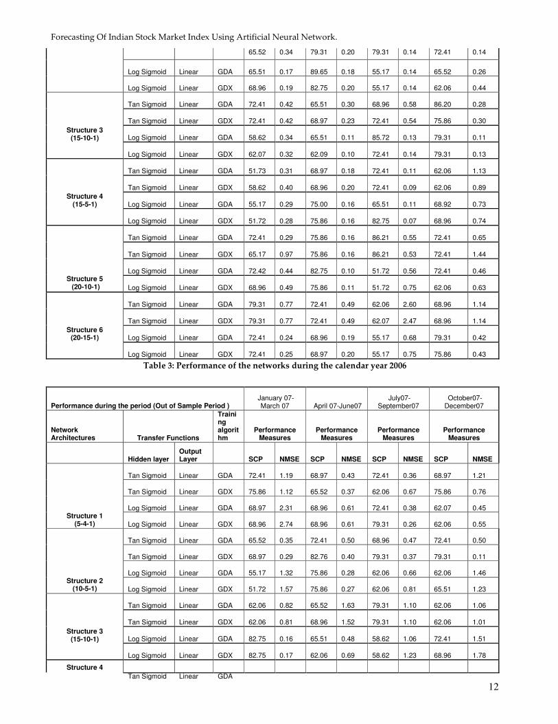
2009. Table 3-6 show the performance of the various networks over a period of 4 years.
Performance during the period (Out of Sample Period ) January 06-
March 06 April 06-June06 July06-
September06 October06-
December06
Network Architectures Transfer Functions
Training algorithm
Performance Measures
Performance Measures
Performance Measures
Performance Measures
Hidden layer Output Layer SCP NMSE SCP NMSE SCP NMSE SCP NMSE
Tan Sigmoid Linear GDA 68.96
0.17
68.97
0.58
68.97
0.65
68.96
0.19
Tan Sigmoid Linear GDX 62.07
0.53
68.97
0.57
68.97
0.59
65.52
0.17
Log Sigmoid Linear GDA 75.86
0.23
79.31
0.34
62.06
0.99
82.75
0.12
Structure 1 (5-4-1) Log Sigmoid Linear GDX
72.31
0.20
82.76
0.32
62.06
1.13
75.86
0.13
Tan Sigmoid Linear GDA 72.41
0.96
79.31
0.20
79.31
0.14
75.86
0.33
Structure 2 (10-5-1)
Tan Sigmoid Linear GDX
Forecasting Of Indian Stock Market Index Using Artificial Neural Network.
12
65.52 0.34 79.31 0.20 79.31 0.14 72.41 0.14
Log Sigmoid Linear GDA 65.51
0.17
89.65
0.18
55.17
0.14
65.52
0.26
Log Sigmoid Linear GDX 68.96
0.19
82.75
0.20
55.17
0.14
62.06
0.44
Tan Sigmoid Linear GDA 72.41
0.42
65.51
0.30
68.96
0.58
86.20
0.28
Tan Sigmoid Linear GDX 72.41
0.42
68.97
0.23
72.41
0.54
75.86
0.30
Log Sigmoid Linear GDA 58.62
0.34
65.51
0.11
85.72
0.13
79.31
0.11
Structure 3 (15-10-1)
Log Sigmoid Linear GDX
62.07
0.32
62.09
0.10
72.41
0.14
79.31
0.13
Tan Sigmoid Linear GDA 51.73
0.31
68.97
0.18
72.41
0.11
62.06
1.13
Tan Sigmoid Linear GDX 58.62
0.40
68.96
0.20
72.41
0.09
62.06
0.89
Log Sigmoid Linear GDA 55.17
0.29
75.00
0.16
65.51
0.11
68.92
0.73
Structure 4 (15-5-1)
Log Sigmoid Linear GDX
51.72
0.28
75.86
0.16
82.75
0.07
68.96
0.74
Tan Sigmoid Linear GDA 72.41
0.29
75.86
0.16
86.21
0.55
72.41
0.65
Tan Sigmoid Linear GDX 65.17
0.97
75.86
0.16
86.21
0.53
72.41
1.44
Log Sigmoid Linear GDA 72.42
0.44
82.75
0.10
51.72
0.56
72.41
0.46
Structure 5 (20-10-1) Log Sigmoid Linear GDX
68.96
0.49
75.86
0.11
51.72
0.75
62.06
0.63
Tan Sigmoid Linear GDA 79.31
0.77
72.41
0.49
62.06
2.60
68.96
1.14
Tan Sigmoid Linear GDX 79.31
0.77
72.41
0.49
62.07
2.47
68.96
1.14
Log Sigmoid Linear GDA 72.41
0.24
68.96
0.19
55.17
0.68
79.31
0.42
Structure 6 (20-15-1)
Log Sigmoid Linear GDX
72.41
0.25
68.97
0.20
55.17
0.75
75.86
0.43
Table 3: Performance of the networks during the calendar year 2006
Performance during the period (Out of Sample Period ) January 07-
March 07 April 07-June07 July07-
September07 October07-December07
Network Architectures Transfer Functions
Training algorithm
Performance Measures
Performance Measures
Performance Measures
Performance Measures
Hidden layer Output Layer SCP NMSE SCP NMSE SCP NMSE SCP NMSE
Tan Sigmoid Linear GDA 72.41
1.19
68.97
0.43
72.41
0.36
68.97
1.21
Tan Sigmoid Linear GDX 75.86
1.12
65.52
0.37
62.06
0.67
75.86
0.76
Log Sigmoid Linear GDA 68.97
2.31
68.96
0.61
72.41
0.38
62.07
0.45
Structure 1 (5-4-1) Log Sigmoid Linear GDX
68.96
2.74
68.96
0.61
79.31
0.26
62.06
0.55
Tan Sigmoid Linear GDA 65.52
0.35
72.41
0.50
68.96
0.47
72.41
0.50
Tan Sigmoid Linear GDX 68.97
0.29
82.76
0.40
79.31
0.37
79.31
0.11
Log Sigmoid Linear GDA 55.17
1.32
75.86
0.28
62.06
0.66
62.06
1.46
Structure 2 (10-5-1) Log Sigmoid Linear GDX
51.72
1.57
75.86
0.27
62.06
0.81
65.51
1.23
Tan Sigmoid Linear GDA 62.06
0.82
65.52
1.63
79.31
1.10
62.06
1.06
Tan Sigmoid Linear GDX 62.06
0.81
68.96
1.52
79.31
1.10
62.06
1.01
Log Sigmoid Linear GDA 82.75
0.16
65.51
0.48
58.62
1.06
72.41
1.51
Structure 3 (15-10-1)
Log Sigmoid Linear GDX
82.75
0.17
62.06
0.69
58.62
1.23
68.96
1.78
Structure 4
Tan Sigmoid Linear GDA
Forecasting Of Indian Stock Market Index Using Artificial Neural Network.
13
62.06 0.21 68.96 0.48 72.41 0.55 65.51 0.57
Tan Sigmoid Linear GDX 62.06
0.21
68.96
0.50
72.41
0.49
65.52
0.55
Log Sigmoid Linear GDA 75.86
0.16
68.96
0.41
51.72
0.51
82.75
0.69 (15-5-1)
Log Sigmoid Linear GDX
75.86
0.16
68.96
0.44
51.72
0.45
79.31
0.49
Tan Sigmoid Linear GDA 79.31
0.18
75.86
1.49
79.31
0.81
72.41
2.27
Tan Sigmoid Linear GDX 82.76
0.34
72.41
1.67
65.51
2.18
72.41
1.42
Log Sigmoid Linear GDA 72.41
0.12
68.96
0.50
75.86
0.43
65.51
2.02
Structure 5 (20-10-1) Log Sigmoid Linear GDX
72.41
0.13
65.51
0.54
75.86
0.43
62.09
2.37
Tan Sigmoid Linear GDA 65.51
0.38
79.31
2.58
65.51
5.70
79.31
3.79
Tan Sigmoid Linear GDX 65.51
0.38
79.31
2.48
65.51
5.70
79.31
3.79
Log Sigmoid Linear GDA 79.31
0.36
72.41
1.22
75.86
1.26
62.06
2.91
Structure 6 (20-15-1)
Log Sigmoid Linear GDX
79.31
0.37
72.41
1.29
75.86
1.17
62.06
3.01
Table 4: Performance of the networks during the calendar year 2006
Performance during the period (Out of Sample Period ) January 08-
March 08 April 08-June08 July08-
September08 October08-December08
Network Architectures Transfer Functions
Training algorithm
Performance Measures
Performance Measures
Performance Measures
Performance Measures
Hidden layer Output Layer SCP NMSE SCP NMSE SCP NMSE SCP NMSE
Tan Sigmoid Linear GDA 62.06
0.54
68.96
0.97
62.06
0.52
65.52
0.52
Tan Sigmoid Linear GDX 62.06
0.54
68.96
1.32
65.96
0.73
65.52
0.52
Log Sigmoid Linear GDA 75.86
0.53
72.41
0.19
62.07
0.99
72.86
0.12
Structure 1 (5-4-1) Log Sigmoid Linear GDX
75.86
0.58
68.96
0.02
62.07
1.14
75.86
0.13
Tan Sigmoid Linear GDA 82.75
0.56
65.52
1.05
68.97
0.58
82.75
0.71
Tan Sigmoid Linear GDX 72.41
1.83
75.86
0.83
79.86
0.35
75.86
0.73
Log Sigmoid Linear GDA 72.41
0.61
68.96
0.26
75.86
0.44
65.71
0.26
Structure 2 (10-5-1) Log Sigmoid Linear GDX
72.41
0.61
72.41
0.29
68.96
0.49
62.09
0.44
Tan Sigmoid Linear GDA 75.86
3.71
62.08
0.22
79.31
2.40
86.20
0.28
Tan Sigmoid Linear GDX 75.86
3.69
62.07
0.75
79.31
2.39
75.86
0.30
Log Sigmoid Linear GDA 75.86
3.36
72.41
0.10
72.41
0.80
79.31
0.11
Structure 3 (15-10-1)
Log Sigmoid Linear GDX
68.96
0.97
72.41
0.11
79.31
0.88
79.31
0.12
Tan Sigmoid Linear GDA 65.71
0.92
72.41
0.19
72.41
1.25
62.07
1.13
Tan Sigmoid Linear GDX 65.71
0.92
68.96
0.16
65.51
1.58
62.07
0.88
Log Sigmoid Linear GDA 72.41
0.07
72.41
0.29
75.86
0.75
68.97
0.73
Structure 4 (15-5-1)
Log Sigmoid Linear GDX
79.31
0.74
68.98
0.26
68.96
0.91
68.96
0.75
Tan Sigmoid Linear GDA 68.96
1.70
62.07
0.85
68.96
0.72
65.52
1.78
Tan Sigmoid Linear GDX 68.96
2.01
62.07
0.65
62.06
1.24
65.51
1.80
Log Sigmoid Linear GDA 72.41
0.97
48.27
0.85
72.41
1.40
72.61
0.46
Structure 5 (20-10-1) Log Sigmoid Linear GDX
72.41
0.97
48.72
0.96
65.51
1.54
62.09
0.63
Forecasting Of Indian Stock Market Index Using Artificial Neural Network.
14
Tan Sigmoid Linear GDA 72.41
3.76
75.86
0.41
58.62
14.31
68.97
1.14
Tan Sigmoid Linear GDX 72.41
3.74
82.76
0.21
58.62
13.95
68.97
1.14
Log Sigmoid Linear GDA 65.17
1.24
79.31
0.20
51.72
5.19
79.31
0.43
Structure 6 (20-15-1)
Log Sigmoid Linear GDX
68.96
1.27
79.31
0.19
51.72
5.11
75.86
0.43
Table 5: Performance of the networks during the calendar year 2006
Performance during the period (Out of Sample Period ) January 09-
March 09 April 09-June09 July09-
September09 October09-December09
Network Architectures Transfer Functions
Training algorithm
Performance Measures
Performance Measures
Performance Measures
Performance Measures
Hidden layer Output Layer SCP NMSE SCP NMSE SCP NMSE SCP NMSE
Tan Sigmoid Linear GDA 72.41
1.79
62.04
0.35
68.97
0.73
75.86
0.59
Tan Sigmoid Linear GDX 72.31
2.14
58.62
0.36
68.97
0.72
72.41
0.58
Log Sigmoid Linear GDA 68.97
1.16
62.09
0.21
68.97
0.44
75.86
0.32
Structure 1 (5-4-1) Log Sigmoid Linear GDX
68.97
1.13
62.06
0.22
68.97
0.45
75.86
0.34
Tan Sigmoid Linear GDA 75.86
0.86
82.75
0.15
65.17
3.59
72.41
1.52
Tan Sigmoid Linear GDX 75.86
1.00
82.75
0.15
55.17
3.02
68.97
1.74
Log Sigmoid Linear GDA 82.76
0.54
75.06
0.12
65.73
1.41
72.41
0.46
Structure 2 (10-5-1) Log Sigmoid Linear GDX
82.76
0.56
75.86
0.12
68.97
1.16
65.51
0.96
Tan Sigmoid Linear GDA 62.07
1.51
68.96
0.38
65.52
3.69
65.51
0.60
Tan Sigmoid Linear GDX 62.07
1.44
68.97
0.38
62.06
3.90
72.41
0.60
Log Sigmoid Linear GDA 68.97
0.36
75.86
0.15
65.52
1.37
68.96
0.28
Structure 3 (15-10-1)
Log Sigmoid Linear GDX
72.41
0.37
79.31
0.15
62.06
1.60
75.86
0.25
Tan Sigmoid Linear GDA 65.52
0.96
65.51
0.38
72.41
1.10
79.31
0.25
Tan Sigmoid Linear GDX 65.52
0.86
65.52
0.41
86.20
0.98
79.31
0.25
Log Sigmoid Linear GDA 65.52
1.01
72.41
0.32
72.41
0.69
72.38
0.24
Structure 4 (15-5-1)
Log Sigmoid Linear GDX
65.52
0.87
68.90
0.36
72.41
0.81
72.41
0.29
Tan Sigmoid Linear GDA 62.07
5.01
65.51
0.78
75.86
1.79
72.41
1.14
Tan Sigmoid Linear GDX 58.62
4.73
65.51
0.80
72.86
1.81
65.71
2.91
Log Sigmoid Linear GDA 62.07
1.11
72.41
0.32
62.06
1.46
62.07
0.39
Structure 5 (20-10-1) Log Sigmoid Linear GDX
62.06
1.30
68.96
0.34
62.06
1.71
68.97
0.41
Tan Sigmoid Linear GDA 65.52
1.42
65.51
1.92
75.86
6.98
58.03
4.09
Tan Sigmoid Linear GDX 65.52
1.47
65.51
1.95
62.09
6.99
58.62
4.09
Log Sigmoid Linear GDA 65.52
1.24
62.06
0.78
75.86
0.94
55.17
1.21
Structure 6 (20-15-1)
Log Sigmoid Linear GDX
65.52
1.20
62.09
0.81
75.86
0.87
51.72
1.39
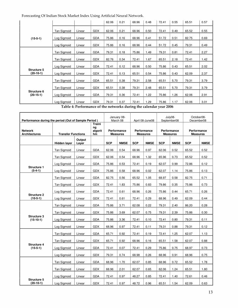
Table 6: Performance of the networks during the calendar year 2006
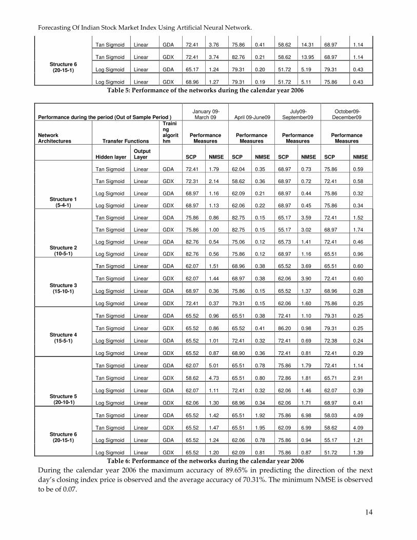
During the calendar year 2006 the maximum accuracy of 89.65% in predicting the direction of the next
day’s closing index price is observed and the average accuracy of 70.31%. The minimum NMSE is observed
to be of 0.07.
Forecasting Of Indian Stock Market Index Using Artificial Neural Network.
15
During the calendar year 2007 the maximum accuracy, in the prediction of the direction of the index, is
observed to be at 82.76%. The average accuracy of for the period is at 69.97%. The minimum NMSE is
observed at 0.11.
The maximum accuracy during the year 2008 is observed to be at 86.20% with average being at 69.85%. The
minimum NMSE is observed at 0.02.
For the year 2009 the maximum accuracy in predicting the direction of the index is observed at 86.20% with
an average to be at 68.74%. The minimum NMSE is observed at 0.12.
From the above results, we are found that the neural network models suggested in the paper is capable of
predicting the direction of the index with an average accuracy of 69.72% and with a maximum of 89.65%.
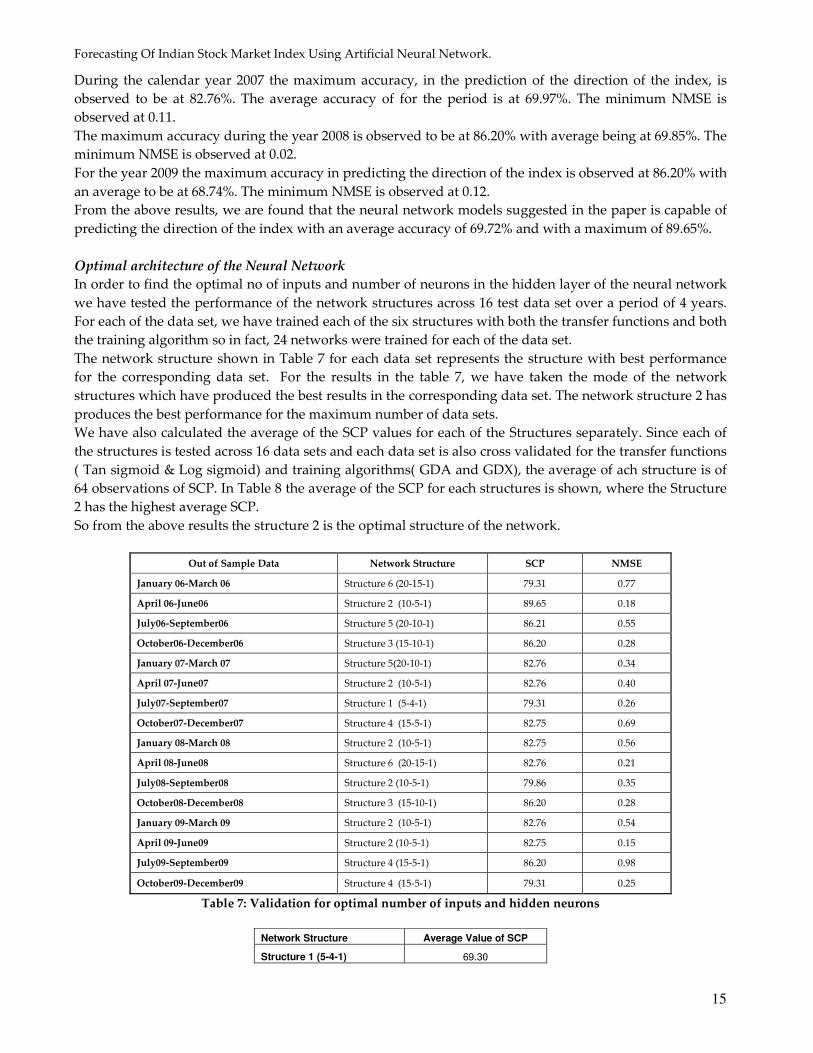
Optimal architecture of the Neural Network
In order to find the optimal no of inputs and number of neurons in the hidden layer of the neural network
we have tested the performance of the network structures across 16 test data set over a period of 4 years.
For each of the data set, we have trained each of the six structures with both the transfer functions and both
the training algorithm so in fact, 24 networks were trained for each of the data set.
The network structure shown in Table 7 for each data set represents the structure with best performance
for the corresponding data set. For the results in the table 7, we have taken the mode of the network
structures which have produced the best results in the corresponding data set. The network structure 2 has
produces the best performance for the maximum number of data sets.
We have also calculated the average of the SCP values for each of the Structures separately. Since each of
the structures is tested across 16 data sets and each data set is also cross validated for the transfer functions
( Tan sigmoid & Log sigmoid) and training algorithms( GDA and GDX), the average of ach structure is of
64 observations of SCP. In Table 8 the average of the SCP for each structures is shown, where the Structure
2 has the highest average SCP.
So from the above results the structure 2 is the optimal structure of the network.
Out of Sample Data Network Structure SCP NMSE
January 06-March 06 Structure 6 (20-15-1) 79.31 0.77
April 06-June06 Structure 2 (10-5-1) 89.65 0.18
July06-September06 Structure 5 (20-10-1) 86.21 0.55
October06-December06 Structure 3 (15-10-1) 86.20 0.28
January 07-March 07 Structure 5(20-10-1) 82.76 0.34
April 07-June07 Structure 2 (10-5-1) 82.76 0.40
July07-September07 Structure 1 (5-4-1) 79.31 0.26
October07-December07 Structure 4 (15-5-1) 82.75 0.69
January 08-March 08 Structure 2 (10-5-1) 82.75 0.56
April 08-June08 Structure 6 (20-15-1) 82.76 0.21
July08-September08 Structure 2 (10-5-1) 79.86 0.35
October08-December08 Structure 3 (15-10-1) 86.20 0.28
January 09-March 09 Structure 2 (10-5-1) 82.76 0.54
April 09-June09 Structure 2 (10-5-1) 82.75 0.15
July09-September09 Structure 4 (15-5-1) 86.20 0.98
October09-December09 Structure 4 (15-5-1) 79.31 0.25
Table 7: Validation for optimal number of inputs and hidden neurons
Network Structure Average Value of SCP
Structure 1 (5-4-1) 69.30
Forecasting Of Indian Stock Market Index Using Artificial Neural Network.
16
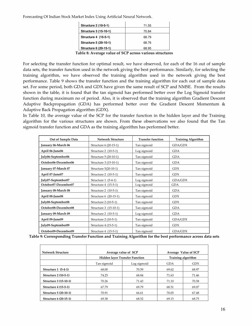
Structure 2 (10-5-1) 71.55
Structure 3 (15-10-1) 70.84
Structure 4 (15-5-1) 68.79
Structure 5 (20-10-1) 68.76
Structure 6 (20-15-1) 68.95
Table 8: Average value of SCP across various structures
For selecting the transfer function for optimal result, we have observed, for each of the 16 out of sample
data sets, the transfer function used in the network giving the best performance. Similarly, for selecting the
training algorithm, we have observed the training algorithm used in the network giving the best
performance. Table 9 shows the transfer function and the training algorithm for each out of sample data
set. For some period, both GDA and GDX have given the same result of SCP and NMSE. From the results
shown in the table, it is found that the tan sigmoid has performed better over the Log Sigmoid transfer
function during maximum no of period. Also, it is observed that the training algorithm Gradient Descent
Adaptive Backpropagation (GDA) has performed better over the Gradient Descent Momentum &
Adaptive Back Propagation algorithm (GDX).
In Table 10, the average value of the SCP for the transfer function in the hidden layer and the Training
algorithm for the various structures are shown. From these observations we also found that the Tan
sigmoid transfer function and GDA as the training algorithm has performed better.
Out of Sample Data Network Structure Transfer function Training Algorithm
January 06-March 06 Structure 6 (20-15-1) Tan sigmoid GDA/GDX
April 06-June06 Structure 2 (10-5-1) Log sigmoid GDA
July06-September06 Structure 5 (20-10-1) Tan sigmoid GDA
October06-December06 Structure 3 (15-10-1) Tan sigmoid GDA
January 07-March 07 Structure 5(20-10-1) Tan sigmoid GDX
April 07-June07 Structure 2 (10-5-1) Tan sigmoid GDX
July07-September07 Structure 1 (5-4-1) Log sigmoid GDA/GDX
October07-December07 Structure 4 (15-5-1) Log sigmoid GDA
January 08-March 08 Structure 2 (10-5-1) Tan sigmoid GDA
April 08-June08 Structure 6 (20-15-1) Tan sigmoid GDX
July08-September08 Structure 2 (10-5-1) Tan sigmoid GDX
October08-December08 Structure 3 (15-10-1) Tan sigmoid GDA
January 09-March 09 Structure 2 (10-5-1) Log sigmoid GDA
April 09-June09 Structure 2 (10-5-1) Tan sigmoid GDA/GDX
July09-September09 Structure 4 (15-5-1) Tan sigmoid GDX
October09-December09 Structure 4 (15-5-1) Tan sigmoid GDA/GDX
Table 9: Corresponding Transfer Function and Training Algorithm for the best performance across data sets
Network Structure Average value of SCP Average Value of SCP
Hidden layer Transfer Function Training algorithm
Tan sigmoid Log sigmoid GDA GDX
Structure 1 (5-4-1) 68.00 70.59 69.62 68.97
Structure 2 (10-5-1) 74.25 68.84 71.63 71.46
Structure 3 (15-10-1) 70.26 71.43 71.10 70.58
Structure 4 (15-5-1) 67.79 69.79 68.51 69.07
Structure 5 (20-10-1) 70.91 66.61 70.05 67.48
Structure 6 (20-15-1) 69.38 68.52 69.15 68.75
Forecasting Of Indian Stock Market Index Using Artificial Neural Network.
17
Average 70.10 69.30 70.01 69.39
Table 10: Average value of SCP for Transfer Function and Training Algorithm across various structures
So from our experiment, a neural network with 10 input variables, 5 hidden neurons and 1 output neuron
with Tan Sigmoid as the transfer function in the hidden layer and Linear transfer function in the output
layer is suggested to be the optimal architecture of Neural network. The Gradient Descent Adaptive Back
Propagation Algorithm is considered as the optimal training algorithm for prediction of the next trading
days closing value of the CNX S&P Nifty 50 Index.
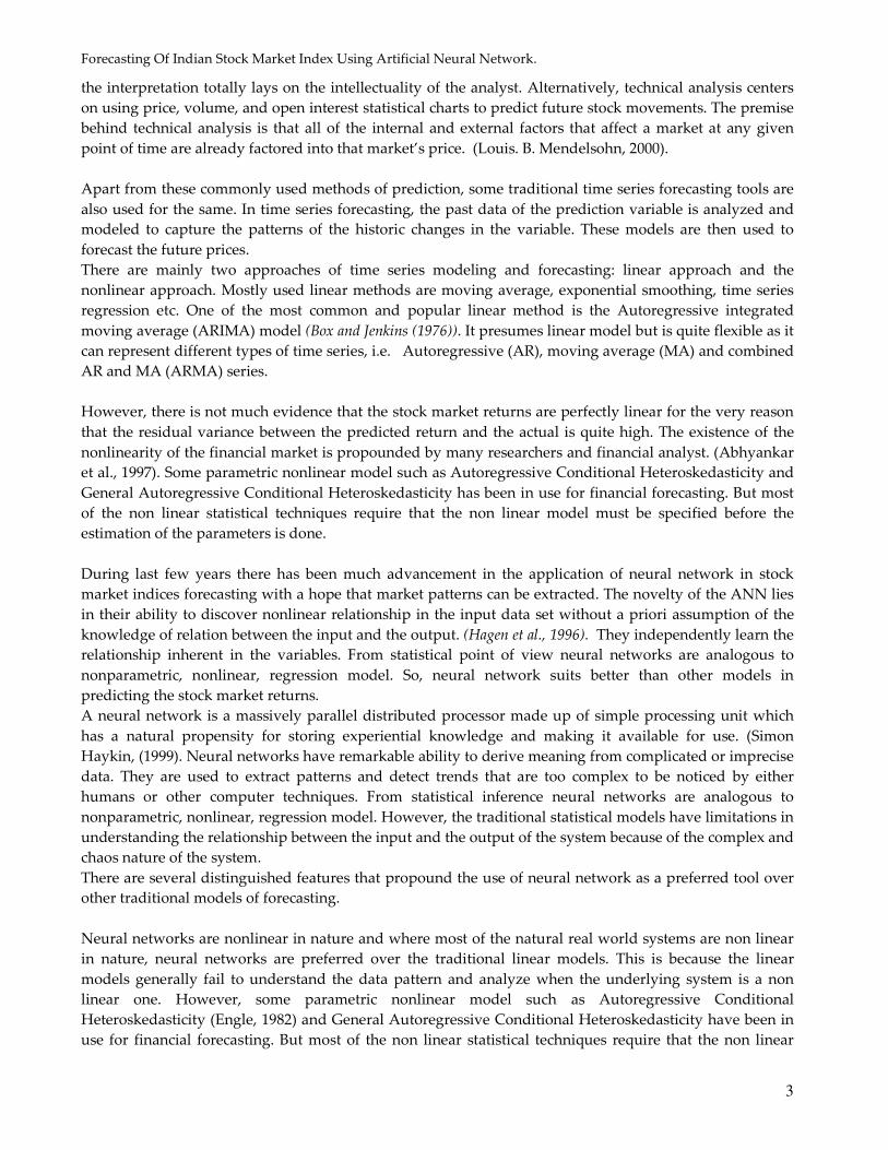
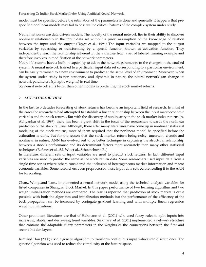
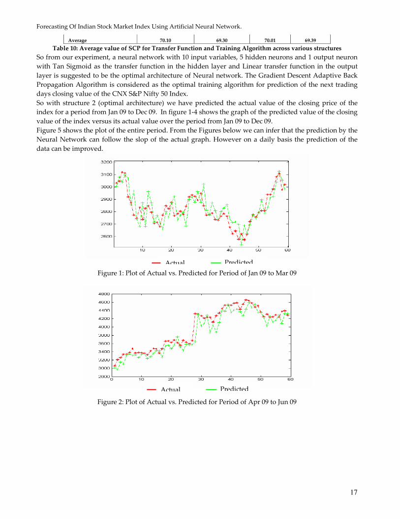
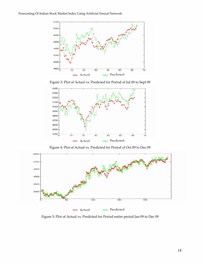
So with structure 2 (optimal architecture) we have predicted the actual value of the closing price of the
index for a period from Jan 09 to Dec 09. In figure 1-4 shows the graph of the predicted value of the closing
value of the index versus its actual value over the period from Jan 09 to Dec 09.
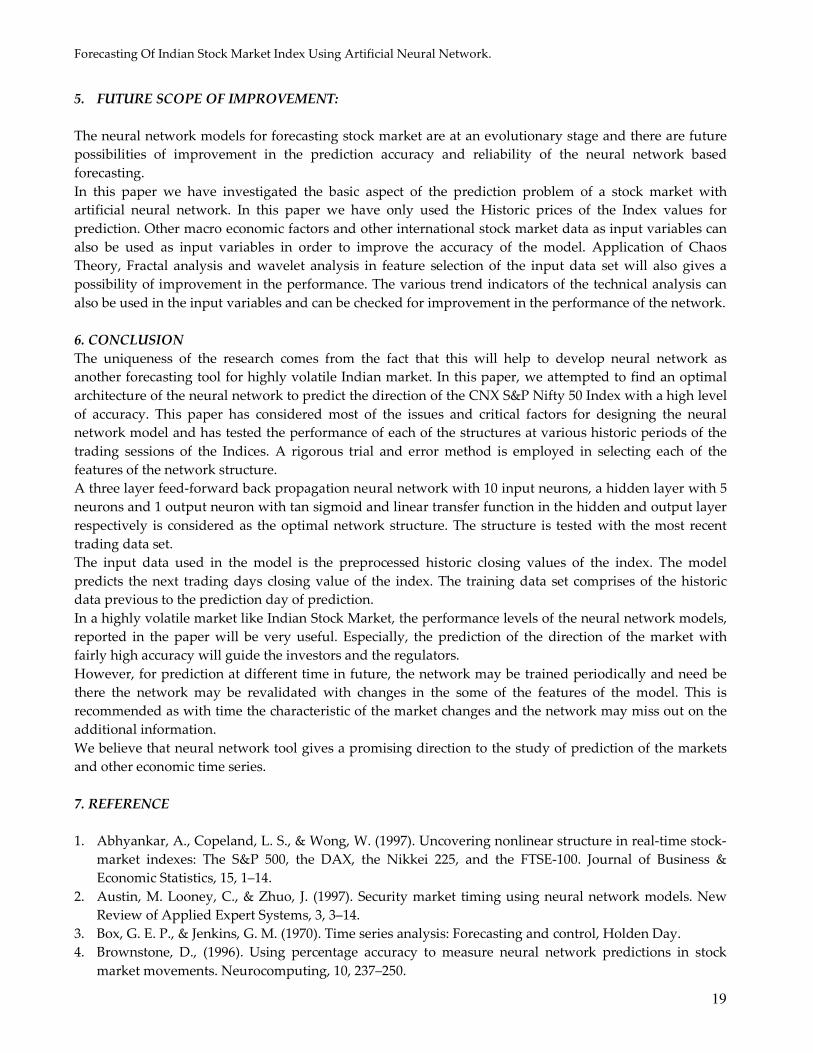
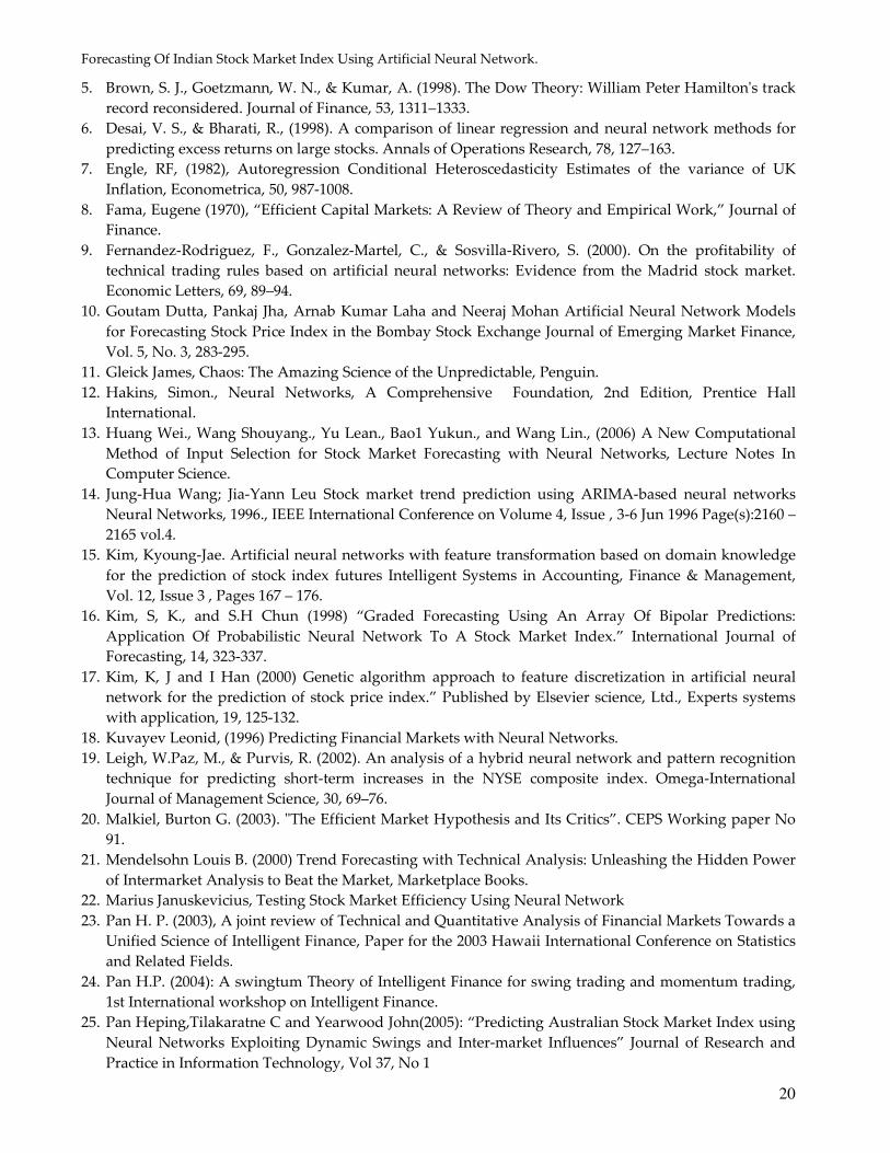
Figure 5 shows the plot of the entire period. From the Figures below we can infer that the prediction by the
Neural Network can follow the slop of the actual graph. However on a daily basis the prediction of the
data can be improved.
Figure 1: Plot of Actual vs. Predicted for Period of Jan 09 to Mar 09
Figure 2: Plot of Actual vs. Predicted for Period of Apr 09 to Jun 09
Actual Predicted
Actual Predicted
Forecasting Of Indian Stock Market Index Using Artificial Neural Network.
18
Figure 3: Plot of Actual vs. Predicted for Period of Jul 09 to Sept 09
Figure 4: Plot of Actual vs. Predicted for Period of Oct 09 to Dec 09
Figure 5: Plot of Actual vs. Predicted for Period entire period Jan 09 to Dec 09
Actual Predicted
Actual Predicted
Actual Predicted
Forecasting Of Indian Stock Market Index Using Artificial Neural Network.
19
5. FUTURE SCOPE OF IMPROVEMENT:
The neural network models for forecasting stock market are at an evolutionary stage and there are future
possibilities of improvement in the prediction accuracy and reliability of the neural network based
forecasting.
In this paper we have investigated the basic aspect of the prediction problem of a stock market with
artificial neural network. In this paper we have only used the Historic prices of the Index values for
prediction. Other macro economic factors and other international stock market data as input variables can
also be used as input variables in order to improve the accuracy of the model. Application of Chaos
Theory, Fractal analysis and wavelet analysis in feature selection of the input data set will also gives a
possibility of improvement in the performance. The various trend indicators of the technical analysis can
also be used in the input variables and can be checked for improvement in the performance of the network.
6. CONCLUSION
The uniqueness of the research comes from the fact that this will help to develop neural network as
another forecasting tool for highly volatile Indian market. In this paper, we attempted to find an optimal
architecture of the neural network to predict the direction of the CNX S&P Nifty 50 Index with a high level
of accuracy. This paper has considered most of the issues and critical factors for designing the neural
network model and has tested the performance of each of the structures at various historic periods of the
trading sessions of the Indices. A rigorous trial and error method is employed in selecting each of the
features of the network structure.
A three layer feed-forward back propagation neural network with 10 input neurons, a hidden layer with 5
neurons and 1 output neuron with tan sigmoid and linear transfer function in the hidden and output layer
respectively is considered as the optimal network structure. The structure is tested with the most recent
trading data set.
The input data used in the model is the preprocessed historic closing values of the index. The model
predicts the next trading days closing value of the index. The training data set comprises of the historic
data previous to the prediction day of prediction.
In a highly volatile market like Indian Stock Market, the performance levels of the neural network models,
reported in the paper will be very useful. Especially, the prediction of the direction of the market with
fairly high accuracy will guide the investors and the regulators.
However, for prediction at different time in future, the network may be trained periodically and need be
there the network may be revalidated with changes in the some of the features of the model. This is
recommended as with time the characteristic of the market changes and the network may miss out on the
additional information.
We believe that neural network tool gives a promising direction to the study of prediction of the markets
and other economic time series.
7. REFERENCE
1. Abhyankar, A., Copeland, L. S., & Wong, W. (1997). Uncovering nonlinear structure in real-time stock-
market indexes: The S&P 500, the DAX, the Nikkei 225, and the FTSE-100. Journal of Business &
Economic Statistics, 15, 1–14.
2. Austin, M. Looney, C., & Zhuo, J. (1997). Security market timing using neural network models. New
Review of Applied Expert Systems, 3, 3–14.
3. Box, G. E. P., & Jenkins, G. M. (1970). Time series analysis: Forecasting and control, Holden Day.
4. Brownstone, D., (1996). Using percentage accuracy to measure neural network predictions in stock
market movements. Neurocomputing, 10, 237–250.
Forecasting Of Indian Stock Market Index Using Artificial Neural Network.
20
5. Brown, S. J., Goetzmann, W. N., & Kumar, A. (1998). The Dow Theory: William Peter Hamilton's track
record reconsidered. Journal of Finance, 53, 1311–1333.
6. Desai, V. S., & Bharati, R., (1998). A comparison of linear regression and neural network methods for
predicting excess returns on large stocks. Annals of Operations Research, 78, 127–163.
7. Engle, RF, (1982), Autoregression Conditional Heteroscedasticity Estimates of the variance of UK
Inflation, Econometrica, 50, 987-1008.
8. Fama, Eugene (1970), “Efficient Capital Markets: A Review of Theory and Empirical Work,” Journal of
Finance.
9. Fernandez-Rodriguez, F., Gonzalez-Martel, C., & Sosvilla-Rivero, S. (2000). On the profitability of
technical trading rules based on artificial neural networks: Evidence from the Madrid stock market.
Economic Letters, 69, 89–94.
10. Goutam Dutta, Pankaj Jha, Arnab Kumar Laha and Neeraj Mohan Artificial Neural Network Models
for Forecasting Stock Price Index in the Bombay Stock Exchange Journal of Emerging Market Finance,
Vol. 5, No. 3, 283-295.
11. Gleick James, Chaos: The Amazing Science of the Unpredictable, Penguin.
12. Hakins, Simon., Neural Networks, A Comprehensive Foundation, 2nd Edition, Prentice Hall
International.
13. Huang Wei., Wang Shouyang., Yu Lean., Bao1 Yukun., and Wang Lin., (2006) A New Computational
Method of Input Selection for Stock Market Forecasting with Neural Networks, Lecture Notes In
Computer Science.
14. Jung-Hua Wang; Jia-Yann Leu Stock market trend prediction using ARIMA-based neural networks
Neural Networks, 1996., IEEE International Conference on Volume 4, Issue , 3-6 Jun 1996 Page(s):2160 –
2165 vol.4.
15. Kim, Kyoung-Jae. Artificial neural networks with feature transformation based on domain knowledge
for the prediction of stock index futures Intelligent Systems in Accounting, Finance & Management,
Vol. 12, Issue 3 , Pages 167 – 176.
16. Kim, S, K., and S.H Chun (1998) “Graded Forecasting Using An Array Of Bipolar Predictions:
Application Of Probabilistic Neural Network To A Stock Market Index.” International Journal of
Forecasting, 14, 323-337.
17. Kim, K, J and I Han (2000) Genetic algorithm approach to feature discretization in artificial neural
network for the prediction of stock price index.” Published by Elsevier science, Ltd., Experts systems
with application, 19, 125-132.
18. Kuvayev Leonid, (1996) Predicting Financial Markets with Neural Networks.
19. Leigh, W.Paz, M., & Purvis, R. (2002). An analysis of a hybrid neural network and pattern recognition
technique for predicting short-term increases in the NYSE composite index. Omega-International
Journal of Management Science, 30, 69–76.
20. Malkiel, Burton G. (2003). "The Efficient Market Hypothesis and Its Critics”. CEPS Working paper No
91.
21. Mendelsohn Louis B. (2000) Trend Forecasting with Technical Analysis: Unleashing the Hidden Power
of Intermarket Analysis to Beat the Market, Marketplace Books.
22. Marius Januskevicius, Testing Stock Market Efficiency Using Neural Network
23. Pan H. P. (2003), A joint review of Technical and Quantitative Analysis of Financial Markets Towards a
Unified Science of Intelligent Finance, Paper for the 2003 Hawaii International Conference on Statistics
and Related Fields.
24. Pan H.P. (2004): A swingtum Theory of Intelligent Finance for swing trading and momentum trading,
1st International workshop on Intelligent Finance.
25. Pan Heping,Tilakaratne C and Yearwood John(2005): “Predicting Australian Stock Market Index using
Neural Networks Exploiting Dynamic Swings and Inter-market Influences” Journal of Research and
Practice in Information Technology, Vol 37, No 1
Forecasting Of Indian Stock Market Index Using Artificial Neural Network.
21
26. Panda, C. and Narasimhan, V. (2006) Predicting Stock Returns : An Experiment of the Artificial Neural
Network in Indian Stock Market South Asia Economic Journal, Vol. 7, No. 2, 205-218.
27. Pantazopoulos, K. N., Tsoukalas, L. H., Bourbakis, N. G., Brun, M. J., & Houstis, E. N. (1998). Financial
prediction and trading strategies using neurofuzzy approaches. IEEE Transactions on Systems, Man,
and Cybernetics-PartB: Cybernetics, 28, 520–530.
28. Roman, Jovina and Jameel, Akhtar Backpropagation and Recurrent Neural Networks in Financial
Analysis of Multiple Stock Market Returns.
29. Refenes, Zapranis, and Francis, (1994) Journal of Neural Networks, Stock Performance Modeling Using
Neural Networks: A Comparative Study with Regression Models, Vol. 7, No. 2,. 375-388.
30. Saad, E.W.; Prokhorov, D.V.; Wunsch, D.C., II (1998) Comparative study of stock trend prediction
using time delay, recurrent and probabilistic neural networks IEEE Transactions on Neural Networks,
Volume 9, Issue 6, Page(s): 1456 - 1470
31. Schoeneburg, E., (1990) Stock Price Prediction Using Neural Networks: A Project Report,
Neurocomputing, vol. 2, 17-27.
32. Siekmann, S., Kruse, R., & Gebhardt, J. (2001). Information fusion in the context of stock index
prediction. International Journal of Intelligent Systems, 16, 1285–1298.
33. S.-I. Wu and H. Zheng (USA) (2003) Can Profits Still be made using Neural Networks in Stock Market?
(410) Applied Simulation and Modeling
34. Tsaih, R., Hsu, Y., & Lai, C. C., (1998). Forecasting S&P 500 stock index futures with a hybrid AI system.
Decision Support Systems, 23, 161–174.
35. Wu S.-I., and Zheng H., (2003). Can Profits Still be Made using Neural Networks in Stock Market?
From Proceeding (410) Applied Simulation and Modeling - 2003