1

Forecasting Directional Changes in Financial Markets

Amer Bakhach, Edward P K Tsang & Wing Lon Ng

Working Paper WP075-15

Centre for Computational Finance and Economic Agents (CCFEA)

University of Essex

8 June 2015

Abstract: Financial forecasting is an important research area. Most researches in forecasting use

time series, which sample market prices at fixed intervals; for example, daily closing prices. Directional

Change (DC) is an alternative approach for sampling market price, which records price changes that the

observer considers significant. The DC approach aims to capture directions price movements – whether

they are on the rise, or in decline. Little forecasting research has been done under the DC framework. In

this paper we formulate a forecasting problem under this framework. In particular, we aim to answer the

question of whether the current trend (up or down) will continue for a particular percentage (which is

decided by the investor) before the trend ends. The success of forecasting depends on the variables that

one uses. In this paper, we introduce three independent variables and prove that they are useful for our

forecasting problem. We show that these variables can help two forecasting algorithms, namely

J48Graft and M5P, to answer the above question. We tested our variables and algorithms in two sets of

data, namely gold price and EUR/USD exchange rates. Experimental results suggest that our approach

outperforms random forecasting in both data sets; in some cases, forecasting accuracy was over 80%.

These results confirm that the independent variables identified are useful for forecasting under the DC

framework.

Keywords: Directional changes, forecasting, Aroon indicator, J48Graft, M5P

1. INTRODUCTION

Forecasting financial time series is a very common objective. Many machine learning approaches

have been introduced for this purpose, in the majority of cases with focus on stock price prediction. To

this end, models have been developed based on Hidden Markov Model (e.g. Hassan & Nath, 2005),

Artificial Neural Network (e.g. White, 1988), Support Vector Machine (e.g. Das & Padhy, 2012) and

Genetic Programming (e.g. Tsang & Li, 2002; Garcia-Almanza & Tsang, 2011). Hybrid methods

merging multiple techniques are also commonly found in the literature. For example, Hassan (2009)

combines a HMM with Fuzzy model; Wang and Leu (1996) propose an ARIMA-based Neural

Networks model, and Yang, Wu, & Lin (2012) propose a hybrid model that combine Genetic Algorithm

with Fuzzy Neural Networks. Iqbal et al. (2013) provide a survey of different state of the art methods

used for stock forecasting. Most research in the literature use interval-based data summaries. In other

words, they sample market prices at fixed time intervals, let it be days, minutes, etc.

Directional Changes (DC) is an alternative approach to summarize market price movements

(Guillaume et al., 1997). Under the DC framework the market is cast into alternating upward trend

(which we call uptrend) and downward trends (which we call downtrend) (Tsang, 2010). Here, a trend

is identified as a market price’s change of a minimum of a given threshold. This threshold, we name it

𝜃, is predefined by the observer; usually expressed as percentage. A trend ends whenever a price change

of same threshold, 𝜃, is observed in the opposite direction. For example, a market downtrend ends when

we observe a price rise of magnitude 𝜃; in this case we say that the market change its direction to

uptrend. Similarly, a market’s uptrend ends when we observe a price decline of magnitude 𝜃; in this

case we say that the market changes its direction to downtrend (see Fig. 1).

In this paper we formulate a novel forecasting problem under the DC framework. The task is to

predict the price at which the trend will reverse. More specifically, we want to forecast whether the

current trend (either uptrend or downtrend) will continue in the same direction for a specific percentage

2

– this percentage is determined by investor. Answering this question is useful for investment decisions;

for example, it could help a trader to decide whether to take a long or short position.

Forecasting crucially depends on the variables that one uses. As a first attempt to tackle this

forecasting problem, we introduce three independent variables in this paper. We attempt to prove that

they are useful for the proposed forecasting problem.

This paper continues as follow: Directional Changes are explained in Section 2. Section 3 provides

the formal definition of our objective. In Section 4 we present our approach for forecasting the end of

trend. We introduce three independent variables and briefly describe two forecasting algorithms.

Section 5 presents details of our experiments in testing our approach. The results are reported in Section

6. The analysis of these findings is discussed in Section 7. We conclude the findings in Section 8.

2. DIRECTIONAL CHANGE (DC)

Directional change (DC) is an alternative way to summarize price changes. In this section, we

explain that, while interval-based summarizes sample market prices at fixed intervals, sampling points

in directional change summaries are data-driven.

Under the DC framework, the market is divided into alternating uptrends and downtrends. Consider

a market in a downtrend. Let 𝑃𝐸𝑋𝑇 be the lowest price in this downtrend and 𝑃𝑐 be the current price. We

say that the market switches its direction from a downtrend to an uptrend whenever 𝑃𝑐 is greater than

the 𝑃𝐸𝑋𝑇 by at least 𝜃, (𝜃 is the threshold pre-determined by the observer). Similarly, if the market is in

an uptrend, 𝑃𝐸𝑋𝑇 would refer to the highest price in this uptrend. We say that the market switches its

direction from an uptrend to a downtrend if 𝑃𝑐 is lower than 𝑃𝐸𝑋𝑇 by at least 𝜃.

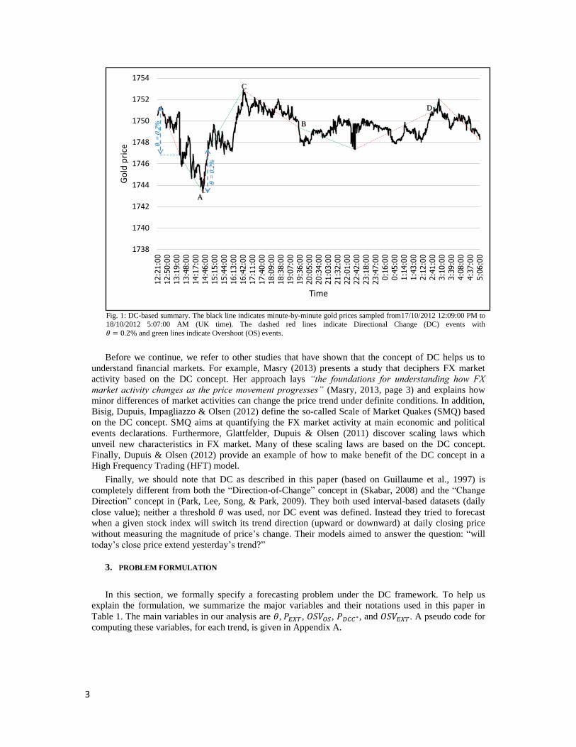
Each trend is composed of a DC event and an overshoot event (see Fig. 1). Formally, a DC event is

detected when we come across a price 𝑃𝑐 that satisfies condition (1). If condition (1) holds, then the time

at which the market traded at 𝑃𝐸𝑋𝑇 is called an ‘extreme point’ (e.g. points A and C in Fig. 1), and the

time at which the market trades at 𝑃𝑐 is called a ‘DC confirmation point’ (e.g. points B and D in Fig. 1).

Note that an extreme point is the end of one trend and it’s also the start of the next trend which has an

opposite direction. The extreme point is only recognized in hindsight – it is recognized precisely at the

DC confirmation point.

|𝑃𝑐 − 𝑃𝐸𝑋𝑇

𝑃𝐸𝑋𝑇

| ≥ 𝜃 (1)

A DC event starts with an extreme point and ends with a DC confirmation point. An overshoot

event (OS event) starts at the DC confirmation point and ends at the next extreme point. A pseudo-code

for defining DC events corresponding to a predetermined threshold 𝜃 can be found in (Glattfelder,

Dupuis, & Olsen, 2011).

It is worth reiterating that we only know the market has changed direction in hindsight; we only

detect a DC event when a DC confirmation point is observed. The question is: could one forecast when

the next DC event will take place? In this paper, we formulate a forecasting problem based on the DC

concept. Given a threshold 𝜃, the task is to forecast, at the DC confirmation point, whether the trend

will change at a certain price.

3

Fig. 1: DC-based summary. The black line indicates minute-by-minute gold prices sampled from17/10/2012 12:09:00 PM to

18/10/2012 5:07:00 AM (UK time). The dashed red lines indicate Directional Change (DC) events with 𝜃 = 0.2% and green lines indicate Overshoot (OS) events.

Before we continue, we refer to other studies that have shown that the concept of DC helps us to

understand financial markets. For example, Masry (2013) presents a study that deciphers FX market

activity based on the DC concept. Her approach lays “the foundations for understanding how FX

market activity changes as the price movement progresses” (Masry, 2013, page 3) and explains how

minor differences of market activities can change the price trend under definite conditions. In addition,

Bisig, Dupuis, Impagliazzo & Olsen (2012) define the so-called Scale of Market Quakes (SMQ) based

on the DC concept. SMQ aims at quantifying the FX market activity at main economic and political

events declarations. Furthermore, Glattfelder, Dupuis & Olsen (2011) discover scaling laws which

unveil new characteristics in FX market. Many of these scaling laws are based on the DC concept.

Finally, Dupuis & Olsen (2012) provide an example of how to make benefit of the DC concept in a

High Frequency Trading (HFT) model.

Finally, we should note that DC as described in this paper (based on Guillaume et al., 1997) is

completely different from both the “Direction-of-Change” concept in (Skabar, 2008) and the “Change

Direction” concept in (Park, Lee, Song, & Park, 2009). They both used interval-based datasets (daily

close value); neither a threshold 𝜃 was used, nor DC event was defined. Instead they tried to forecast

when a given stock index will switch its trend direction (upward or downward) at daily closing price

without measuring the magnitude of price’s change. Their models aimed to answer the question: “will

today’s close price extend yesterday’s trend?”

3. PROBLEM FORMULATION

In this section, we formally specify a forecasting problem under the DC framework. To help us

explain the formulation, we summarize the major variables and their notations used in this paper in

Table 1. The main variables in our analysis are 𝜃, 𝑃𝐸𝑋𝑇 , 𝑂𝑆𝑉𝑂𝑆, 𝑃𝐷𝐶𝐶∗, and 𝑂𝑆𝑉𝐸𝑋𝑇 . A pseudo code for

computing these variables, for each trend, is given in Appendix A.

1738

1740

1742

1744

1746

1748

1750

1752

1754

12:21:00

12:50:00

13:19:00

13:48:00

14:17:00

14:46:00

15:15:00

15:44:00

16:13:00

16:42:00

17:11:00

17:40:00

18:09:00

18:38:00

19:07:00

19:36:00

20:05:00

20:34:00

21:03:00

21:32:00

22:01:00

22:42:00

23:18:00

23:47:00

0:16:00

0:45:00

1:14:00

1:43:00

2:12:00

2:41:00

3:10:00

3:39:00

4:08:00

4:37:00

5:06:00

Go

ld p

rice

Time

𝜃=

0.2

%

𝜃=

0.2

%

A

C

B

D

4

Table 1: List of notations used in this paper.

Name / Description Notation

Threshold 𝜃

Current price 𝑃𝑐

Price at extreme point: price at which one trend ends and a new trend starts (e.g.

points A, C in Fig. 1) 𝑃𝐸𝑋𝑇

Lowest price at an uptrend DC confirmation point: The least price change required at a downtrend to confirm that direction has changed to an uptrend

𝑃𝐷𝐶𝐶∗ = 𝑃𝐸𝑋𝑇 × ( 1 + 𝜃)

Highest price at a downtrend DC confirmation point: The least price change

required at an uptrend to confirm that direction has changed to a downtrend 𝑃𝐷𝐶𝐶∗ = 𝑃𝐸𝑋𝑇 × ( 1 − 𝜃)

Overshoot value (OSV) at any point:

At the DC confirmation point (e.g. point B, D in Fig. 1) we name it 𝑂𝑆𝑉𝑂𝑆

At the end of an OS event (e.g. points A, C in Fig. 1) we name it 𝑂𝑆𝑉𝐸𝑋𝑇

𝑂𝑆𝑉 = ((𝑃𝑐 − 𝑃𝐷𝐶𝐶∗) ÷ 𝑃𝐷𝐶𝐶∗) ÷ 𝜃

We stipulate that the ith trend starts at 𝑃𝐸𝑋𝑇𝑖 and ends at 𝑃𝐸𝑋𝑇

𝑖+1 . We denote the OSV at 𝑃𝐸𝑋𝑇𝑖+1 with

𝑂𝑆𝑉𝐸𝑋𝑇𝑖 because it is computed at the end of the OS event of the ith trend (not the (i+1)th trend).

Clearly, there is a lot of incentive to predict 𝑃𝐸𝑋𝑇𝑖+1 . In this paper, we choose to forecast on 𝑂𝑆𝑉𝐸𝑋𝑇

𝑖 .

The attractiveness of forecasting 𝑂𝑆𝑉𝐸𝑋𝑇𝑖 instead of 𝑃𝐸𝑋𝑇

𝑖+1 is that the former is a relative value (relative to

θ, which is the user’s measure of significance) while the latter is an absolute value. Relative values are

comparable between series. By forecasting 𝑂𝑆𝑉𝐸𝑋𝑇𝑖 , we are effectively forecasting 𝑃𝐸𝑋𝑇

𝑖+1 because:

𝑃𝐸𝑋𝑇𝑖+1 = 𝑃𝐷𝐶𝐶∗

𝑖 × (1 + 𝑂𝑆𝑉𝐸𝑋𝑇𝑖 × 𝜃) (2)

We adopt the following notation throughout this paper: we use 𝑂𝑆𝑉𝐸𝑋𝑇 to denote the vector

containing all 𝑂𝑆𝑉𝐸𝑋𝑇𝑖 for all the trends. The same convention applies to other variables 𝑃𝐸𝑋𝑇, 𝑂𝑆𝑉𝑂𝑆,

and 𝑃𝐷𝐶𝐶∗. It is worth reiterating that directional changes can only be confirmed in hindsight. Therefore,

at the DC confirmation point of ith trend we can compute 𝑃𝐷𝐶𝐶∗𝑖 but not 𝑂𝑆𝑉𝐸𝑋𝑇

𝑖 , hence the above

forecasting problem.

We formulate the problem as a Boolean forecasting problem. At the DC confirmation point of the ith

trend, we would like to predict whether 𝑂𝑆𝑉𝐸𝑋𝑇𝑖 < 𝑑 for a constant 𝑑. Note that based on Equation (2)

we can deduce rule (3):

𝑖𝑓 (𝑂𝑆𝑉𝐸𝑋𝑇𝑖 < 𝑑 ), 𝑡ℎ𝑒𝑛 𝑃𝐸𝑋𝑇

𝑖+1 < 𝑃𝐷𝐶𝐶∗𝑖 × ( 1 + 𝑑 × 𝜃) (3)

In addition, if we replace 𝑂𝑆𝑉𝐸𝑋𝑇𝑖 with 𝑑 in Equation (2), then we can obtain Equation (4):

((𝑃𝐸𝑋𝑇𝑖+1 − 𝑃𝐷𝐶𝐶∗

𝑖 ) ÷ 𝑃𝐷𝐶𝐶∗𝑖 ) = 𝑑 × 𝜃 (4)

Why is this forecasting problem worth studying? According to Table 1, the price at the ith DC

confirmation point is approximately equal to 𝑃𝐷𝐶𝐶∗𝑖 . Suppose the ith trend is an uptrend (the arguments in

a downtrend is similar). If a trader takes a long position at the ith DC confirmation point and closes the

position at the forecasted price 𝑃𝐸𝑋𝑇𝑖+1 , then 𝑑 × 𝜃 represents the expected profit (see Equation 4). Hence,

the trader can use 𝑑 to control the profit target.

4. APPROACH TO FORECASTING END OF TREND

In the previous section, we have explained that our task is to predict whether 𝑂𝑆𝑉𝐸𝑋𝑇𝑖 < 𝑑. In this

section we provide a novel approach to answer this problem. Note that forecasting 𝑂𝑆𝑉𝐸𝑋𝑇𝑖 to be less

than 𝑑 is equivalent to predicting that the current ith trend, assumed to be an uptrend, will reverse at

price less than 𝑃𝐸𝑋𝑇𝑖+1 which is computed according to rule (3) (i.e. we predict that the next DC event will

occur before the price reaches (1 + 𝑑 × 𝜃) above the price 𝑃𝐷𝐶𝐶∗𝑖 of the current trend). Similar

conclusion can be made for a downtrend.

Forecasting is only possible if one can define the target variable which value we attempt to predict.

We also need to identify variables that the target variable is dependent on. Therefore, our first

5

challenge is to define a variable that represents the question “is 𝑂𝑆𝑉𝐸𝑋𝑇𝑖 < 𝑑 𝑇𝑟𝑢𝑒?”. Then we shall

introduce variables that could help us to answer this question. Finally, we shall describe two forecasting

algorithms for testing the relevance of these variables.

4.1. Chosen variables

We define the Boolean variable 𝐵𝑂𝑆𝑉𝐸𝑋𝑇 as the target variable in our forecasting problem. Our task

is to forecasting whether 𝐵𝑂𝑆𝑉𝐸𝑋𝑇𝑖 is 𝑇𝑟𝑢𝑒 or 𝐹𝑎𝑙𝑠𝑒, as defined in Expression (5). The value of

𝐵𝑂𝑆𝑉𝐸𝑋𝑇𝑖 depends on the value of the unknown variable 𝑂𝑆𝑉𝐸𝑋𝑇

𝑖 and the constant 𝑑:

(𝐵𝑂𝑆𝑉𝐸𝑋𝑇𝑖 = 𝑇𝑟𝑢𝑒) 𝑖𝑓 𝑎𝑛𝑑 𝑜𝑛𝑙𝑦 𝑖𝑓(𝑂𝑆𝑉𝐸𝑋𝑇

𝑖 < 𝑑), 𝑒𝑙𝑠𝑒 (𝐵𝑂𝑆𝑉𝐸𝑋𝑇𝑖 = 𝐹𝑎𝑙𝑠𝑒) (5)

How could one predict the value of 𝐵𝑂𝑆𝑉𝐸𝑋𝑇𝑖 ? Identifying appropriate independent variables for a

given forecasting problem is non-trivial in general. Our task is particularly difficult because existing

technical indicators for interval-based summaries are not compatible with the DC framework. For

example, Ehlers’s leading indicator (ELI) (Ehlers, 2002), Aroon indicator (Chande & Kroll, 1994),

Relative Strength Index (RSI) and average directional movement index (ADX) (Wilder, 1978) in their

original form cannot be applied to the DC framework, as they assume that data are sampled at fixed

intervals. Below we present three variables which could be used to predict the value of 𝐵𝑂𝑆𝑉𝐸𝑋𝑇𝑖 .

The first two variables derive from the Aroon trend indicator (Chande & Kroll, 1994). These two

variables are: 𝐴𝑟𝑜𝑜𝑛𝑈𝑝(𝑛) and 𝐴𝑟𝑜𝑜𝑛𝐷𝑜𝑤𝑛(𝑛), which we define below. Generally, the Aroon

indicators are applied to a financial time series to identify trends and the probability that the trends will

reverse.

Suppose 𝑃0, 𝑃1, 𝑃2, … are observations of prices in the market. At observation 𝑃𝑡−0, 𝐴𝑟𝑜𝑜𝑛𝑈𝑝(𝑛)

and 𝐴𝑟𝑜𝑜𝑛𝐷𝑜𝑤𝑛(𝑛) are defined with reference to the previous 𝑛 observations, together with the

current observation 𝑃𝑡−0. In other words, we focus on a period of 𝑛 + 1 observations, with prices

𝑃𝑡−𝑛 , … , 𝑃𝑡−1, 𝑃𝑡−0 where 𝑛 is a parameter to the indicator. Here, 𝑃𝑡−𝑛 is the earliest observation in the

period and 𝑃𝑡−0 is the latest observation. Let 𝑚 and 𝑚′ be two indices such that 𝑃𝑡−𝑚 and 𝑃𝑡−𝑚′ are the

most recent highest price and lowest price respectively in this period; i.e. for all i in 0... 𝑛, we have

𝑃𝑡−𝑚 ≥ 𝑃𝑡−𝑖, 𝑃𝑡−𝑚′ ≤ 𝑃𝑡−𝑖. If there exists another index j (with j in 0... 𝑛) such that 𝑃𝑡−𝑚 = 𝑃𝑡−𝑗

then 𝑚 < 𝑗; the same applies for 𝑚′(i.e. if there exists another index k, with k in 0... 𝑛, such

that 𝑃𝑡−𝑚′ = 𝑃𝑡−𝑘 then 𝑚′ < k). The formula corresponding to 𝐴𝑟𝑜𝑜𝑛𝑈𝑝(𝑛) is defined in Equation (6):

𝐴𝑟𝑜𝑜𝑛𝑈𝑝(𝑛) = (( 𝑛 − 𝑚 ) ÷ 𝑛) × 100 (6)

For example, let 𝑛 = 3. If 𝑃𝑡−3 = 101, 𝑃𝑡−2 = 102, 𝑃𝑡−1 = 103, 𝑃𝑡−0 = 10, then 𝑚 = 0 (because

104 is the highest price in this window). If 𝑃𝑡−3 = 104, 𝑃𝑡−2 = 102, 𝑃𝑡−1 = 106, 𝑃𝑡−0 = 104, then

𝑚 = 1 (because 106 is the highest price in this window). If 𝑃𝑡−3 = 104, 𝑃𝑡−2 = 102, 𝑃𝑡−1 = 104,

𝑃𝑡−0 = 104, then 𝑚 = 0 (because 104 is the highest price in this window, but 𝑃𝑡−0 is the most recent).

If 𝑃𝑡−3 = 104, 𝑃𝑡−2 = 102, 𝑃𝑡−1 = 103, 𝑃𝑡−0 = 101, then 𝑚 = 3. 𝐴𝑟𝑜𝑜𝑛𝐷𝑜𝑤𝑛(𝑛) is computed

exactly as the opposite mode, searching for lowest price instead of highest price. The formula

corresponding to 𝐴𝑟𝑜𝑜𝑛𝐷𝑜𝑤𝑛(𝑛) is Equation (7). The 𝐴𝑟𝑜𝑜𝑛𝑈𝑝(𝑛) and 𝐴𝑟𝑜𝑜𝑛𝐷𝑜𝑤𝑛(𝑛) values are

bounded between 0 and 100:

𝐴𝑟𝑜𝑜𝑛𝐷𝑜𝑤𝑛(𝑛) = (( 𝑛 − 𝑚′ ) ÷ 𝑛) × 100 (7)

In our case, we want to compute the 𝐴𝑟𝑜𝑜𝑛𝑈𝑝(𝑛) and 𝐴𝑟𝑜𝑜𝑛𝐷𝑜𝑤𝑛(𝑛) variables under the DC

context. To adapt these two variables to the DC concept we provide the following indications and

examples:

We define an observation per trend. Each observation comprises the two prices corresponding

to the start and the end of a DC event. More explicitly, an observation is a couple of prices: the

price at which a DC event starts, i.e. 𝑃𝐸𝑋𝑇 , and the price at DC confirmation point, i.e. price at

which the OS event starts (see Section 2).

6

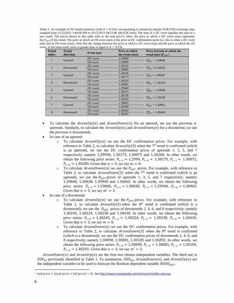
Table 2: An example of DC-based summary (with 𝜃 = 0.1%) corresponding to minute-by-minute EUR/USD exchange rates

sampled from 15/12/2011 3:44:00 PM to 16/12/2011 04:53:00 AM (UK time). The start of a DC event signifies the start of a

new trend. The prices shown in this table refer to the mid price1). Here, the price at which a DC event starts represents

the 𝑃𝐸𝑋𝑇 of this trend. The price at which an OS event starts is the price at DC confirmation point (i.e. this is when a DC event

ends and an OS event starts). Note that the change between the price at which a DC event starts and the price at which the OS

event, of the same trend, starts is greater than or equal to 𝜃 = 0.1%.

Trend

index

Trend

direction Event type

Price at which

the event starts

Price extreme at which the

trend start (𝑷𝑬𝑿𝑻)

1 Upward DC event 1.29840

𝑃𝐸𝑋𝑇1 = 1.29840

OS event 1.29990

2 Downward DC event 1.30245

𝑃𝐸𝑋𝑇2 =1.30245

OS event 1.30090

3 Upward DC event 1.30038

𝑃𝐸𝑋𝑇3 = 1.30038

OS event 1.30175

4 Downward DC event 1.30224

𝑃𝐸𝑋𝑇4 = 1.30224

OS event 1.30081

5 Upward DC event 1.29940

𝑃𝐸𝑋𝑇5 = 1.29940

OS event 1.30072

6 Downward DC event 1.30238

𝑃𝐸𝑋𝑇6 = 1.30238

OS event 1.30105

7 Upward DC event 1.30065

𝑃𝐸𝑋𝑇7 = 1.30065

OS event 1.30200

8 Downward DC event 1.30430

𝑃𝐸𝑋𝑇8 = 1.30430

OS event 1.30293

To calculate the 𝐴𝑟𝑜𝑜𝑛𝑈𝑝(𝑛) and 𝐴𝑟𝑜𝑜𝑛𝐷𝑜𝑤𝑛(𝑛) for an uptrend, we use the previous 𝑛 uptrends. Similarly, to calculate the 𝐴𝑟𝑜𝑜𝑛𝑈𝑝(𝑛) and 𝐴𝑟𝑜𝑜𝑛𝐷𝑜𝑤𝑛(𝑛) for a downtrend, we use

the previous 𝑛 downtrends.

In case of an uptrend:

o To calculate 𝐴𝑟𝑜𝑜𝑛𝑈𝑝(𝑛) we use the DC confirmation prices. For example, with

reference to Table 2, to calculate 𝐴𝑟𝑜𝑜𝑛𝑈𝑝(3) when the 7th trend is confirmed (which

is an uptrend), we use the DC confirmation prices of uptrends 1, 3, 5, and 7

respectively; namely 1.29990, 1.30175, 1.30072 and 1.30200. In other words, we

obtain the following price series: 𝑃𝑡−3 = 1.2999, 𝑃𝑡−2 = 1.30175, 𝑃𝑡−1 = 1.30072, 𝑃𝑡−0 = 1.30200. Given that 𝑛 = 3, we say 𝑚 = 0.

o To calculate 𝐴𝑟𝑜𝑜𝑛𝐷𝑜𝑤𝑛(𝑛) we use the 𝑃𝐸𝑋𝑇 prices. For example, with reference to

Table 2, to calculate 𝐴𝑟𝑜𝑜𝑛𝐷𝑜𝑤𝑛(3) when the 7th trend is confirmed (which is an

uptrend), we use the 𝑃𝐸𝑋𝑇 prices of uptrends 1, 3, 5, and 7 respectively; namely

1.29840, 1.30038, 1.29940 and 1.30065. In other words, we obtain the following

price series: 𝑃𝑡−3 = 1.29840, 𝑃𝑡−2 = 1.30038, 𝑃𝑡−1 = 1.29940, 𝑃𝑡−0 = 1.30065. Given that 𝑛 = 3, we say 𝑚′ = 3.

In case of a downtrend:

o To calculate 𝐴𝑟𝑜𝑜𝑛𝑈𝑝(𝑛) we use the 𝑃𝐸𝑋𝑇 prices. For example, with reference to

Table 2, to calculate 𝐴𝑟𝑜𝑜𝑛𝑈𝑝(3) when the 8th trend is confirmed (which is a

downtrend), we use the 𝑃𝐸𝑋𝑇 prices of downtrends 2, 4, 6, and 8 respectively; namely

1.30245, 1.30224, 1.30238 and 1.30430. In other words, we obtain the following

price series: 𝑃𝑡−3 = 1.30245, 𝑃𝑡−2 = 1.30224, 𝑃𝑡−1 = 1.30238, 𝑃𝑡−0 = 1.30430.

Given that 𝑛 = 3, we say 𝑚 = 0. o To calculate 𝐴𝑟𝑜𝑜𝑛𝐷𝑜𝑤𝑛(𝑛) we use the DC confirmation prices. For example, with

reference to Table 2, to calculate 𝐴𝑟𝑜𝑜𝑛𝐷𝑜𝑤𝑛(3) when the 8th trend is confirmed

(which is a downtrend), we use the DC confirmation prices of downtrends 2, 4, 6, and

8 respectively; namely 1.30090, 1.30081, 1.30105 and 1.30293. In other words, we

obtain the following price series: 𝑃𝑡−3 = 1.30090, 𝑃𝑡−2 = 1.30081, 𝑃𝑡−1 = 1.30105, 𝑃𝑡−0 = 1.30293. Given that 𝑛 = 3, we say 𝑚′ = 2.

𝐴𝑟𝑜𝑜𝑛𝐷𝑜𝑤𝑛(𝑛) and 𝐴𝑟𝑜𝑜𝑛𝑈𝑝(𝑛) are the first two chosen independent variables. The third one is

𝑂𝑆𝑉𝑂𝑆 previously identified in Table 1. To summarize, 𝑂𝑆𝑉𝑂𝑆, 𝐴𝑟𝑜𝑜𝑛𝐷𝑜𝑤𝑛(𝑛), and 𝐴𝑟𝑜𝑜𝑛𝑈𝑝(𝑛) are

the independent variables to be used to forecast the Boolean dependent variable 𝐵𝑂𝑆𝑉𝐸𝑋𝑇 .

1 𝑚𝑖𝑑 𝑝𝑟𝑖𝑐𝑒 = ((𝑎𝑠𝑘 𝑝𝑟𝑖𝑐𝑒 + 𝑏𝑖𝑑 𝑝𝑟𝑖𝑐𝑒) ÷ 2). See http://www.investopedia.com/terms/m/middle-rate.asp.

7

4.2. Algorithms: J48Graft and M5P

According to rule (5), our objective is to predict whether 𝐵𝑂𝑆𝑉𝐸𝑋𝑇𝑖 is 𝑇𝑟𝑢𝑒 or 𝐹𝑎𝑙𝑠𝑒. Such an

objective can be seen as a classification task. For this purpose, we have chosen to use two machine

learning algorithms in the literature: J48Graft and M5P.2 Both algorithms belong to the decision tree

classifier family. In this Section we provide a brief review about each algorithm.

J48 is the open-source Java implementation of C4.5 algorithm (Witten, Frank, & Hall, 2011). C4.5

algorithm descends from the simple divide-and-conquer algorithm for generating decision trees

(Quinlan, 1993). J48 has three main steps. First, for each attribute λ it computes the normalized

information gain ratio from splitting on λ. Let λ_best be the attribute with the highest normalized

information gain. Second, it creates a decision node nd that splits on λ_best. Third, it recurs on the

sublists obtained by splitting on λ_best, and add those nodes as children of node nd. The three steps are

repeated until a base case is reached. This algorithm has multiple base cases (see Quinlan, 1993).

The J48Graft algorithm is an enhanced version of J48 (Webb, 1999). It adds nodes to a given

decision tree in aim of reducing the prediction tree. It considers alternative classification for regions of

the sample space that are not occupied by training examples. “These classifications are generated by

considering alternative branches based on the predecessor nodes to the leaf contained those identified

region.” (Kokar, Venkatesan, Tandel, & Palivela, 2014, page 409). Finally, J48Graft has been reported

to have better accuracy than J48 (Rajput & Arora, 2013).

M5P is a regression tree classifier based on the M5 algorithm for inducing trees of regression

models (Quinlan, 1992). M5P is a model tree algorithm. It generates regression trees whose leaves are

union of multivariate linear models. First, a decision-tree induction algorithm is applied to generate a

tree. M5P uses a splitting criterion that minimizes the intra-subset variation in the class values down

each branch. The splitting process repeats until the class values of all instances that reach a node differ

marginally, or only a few instances remain. Second, after a tree is constructed, a bottom-up pruning

algorithm is conducted. When pruning, an internal node becomes a leaf with a regression plane by

computing the expected error for test data. Third, to remove severe discontinuities between the subtrees

a smoothing procedure is applied that combines the leaf model prediction with each node along the path

back to the root. Smoothing can be achieved by producing linear models for each internal node, as well

as for the leaves, at the time the tree is built (Wang & Witten, 1997).

There are other methods for building decision trees. For example, genetic programming has been

demonstrated to be useful for building decision trees in financial forecasting (Tsang & Li, 2002). The

repository method and its variances have been found effective in post-processing decision trees to

improve their performance (Jin, Tsang, & Li, 2009).

In this section, we have described the basic elements of our approach: the independent variables and

two selected forecasting algorithms. Next, the performance of our approach is examined

experimentally.

5. EXPERIMENTS

In order to verify whether 𝐵𝑂𝑆𝑉𝐸𝑋𝑇 is predictable using the independent variables and the machine

learning algorithms that we have chosen, we provide four sets of experiments. In the first set of

experiments, we use minute-by-minute gold prices in order to test whether our approach can outperform

random forecast. In the second set of experiments, we test whether the performance observed in the first

set of experiments can be attained in another market; for this purpose, we apply our approach to another

dataset composed of minute-by-minute EUR/USD exchange rate. The third set of experiments tests the

significance of each of the selected independent variables identified in Section 4.1. The fourth set of

experiments aims to examine the sensitivity of our approach to the choice of the Aroon indicator

parameter 𝑛.

2 In preliminary experiments, we have tried other algorithms: ID3, ADTree, J48, and CART (Witten, Frank, & Hall, 2011). J48Graft

and M5P show better accuracy than the others.

8

5.1. Performance of our forecasting approach in gold prices

To assess the performance of our forecasting approach, we apply it to minute-by-minute time series

of gold price during the period from 16/10/2012 18:56:00 to 07/04/2014 13:54:00 (UK time) consisting

of a total of 531308 observations. After running DC based analysis (see Appendix A) with a threshold

of θ = 0.2%, we count 6464 trends. For each trend we compute the four variables: 𝑂𝑆𝑉𝑂𝑆,

𝐴𝑟𝑜𝑜𝑛𝑈𝑝(𝑛), 𝐴𝑟𝑜𝑜𝑛𝐷𝑜𝑤𝑛(𝑛) and 𝑂𝑆𝑉𝐸𝑋𝑇 . These variables constitute our new dataset Ḏ.

Based on the instructions provided in Section 4.1, concerning how to compute 𝐴𝑟𝑜𝑜𝑛𝐷𝑜𝑤𝑛(𝑛),

and 𝐴𝑟𝑜𝑜𝑛𝑈𝑝(𝑛) in the DC context, we use uptrends to predict 𝐵𝑂𝑆𝑉𝐸𝑋𝑇 in uptrends, and downtrends

to predict 𝐵𝑂𝑆𝑉𝐸𝑋𝑇 in downtrends. Therefore, we split our dataset Ḏ into two dataset ḎA and ḎB where

ḎA represents the set of downward trends and ḎB represents the set of upward trends. Each of ḎA and ḎB

contains 3232 observations. In this set of experiments, we focus on the downward trends dataset ḎA. ḎB

is processed similarly.

Next, we set, arbitrarily, 𝑛 = 20 in Equations (6) and (7) to compute 𝐴𝑟𝑜𝑜𝑛𝐷𝑜𝑤𝑛(𝑛),

and 𝐴𝑟𝑜𝑜𝑛𝑈𝑝(𝑛)3. Consequently, we eliminate the first 20 observations of ḎA because they have

neither 𝐴𝑟𝑜𝑜𝑛𝑈𝑝(𝑛) nor 𝐴𝑟𝑜𝑜𝑛𝐷𝑜𝑤𝑛(𝑛) values. Finally, we obtain 3212 downward trends in ḎA.

The dependent variable 𝐵𝑂𝑆𝑉𝐸𝑋𝑇 is defined with reference to 𝑑 (see rule (5)). We have tried 11

different values corresponding to 11 quantile values: (𝑑 =q25, q30, q35, q40, q45, q50, q55, q60, q65, q70, q75)

where qj is the number at which j % of 𝑂𝑆𝑉𝐸𝑋𝑇 observations are less than qj. Hence, we get 11 different

datasets 𝐷𝑗𝐴 (j=25, 30, 35,…, 75). In other words, if we apply rule (5) we should have j % of

𝐵𝑂𝑆𝑉𝐸𝑋𝑇values being 𝑇𝑟𝑢𝑒 in the dataset 𝐷𝑗𝐴. For each dataset we replace the variable 𝑂𝑆𝑉𝐸𝑋𝑇 with the

corresponding variable 𝐵𝑂𝑆𝑉𝐸𝑋𝑇 computed based on rule (5). All these datasets have exactly same

values of the three independent variables. They only differ by the dependent variable 𝐵𝑂𝑆𝑉𝐸𝑋𝑇 which

can be only 𝑇𝑟𝑢𝑒 or 𝐹𝑎𝑙𝑠𝑒 according to the value of parameter 𝑑 as described in rule (5). These

datasets are used to test the performance of the learning algorithms given different level of 𝑇𝑟𝑢𝑒-

𝐹𝑎𝑙𝑠𝑒 imbalance in the dependent variable 𝐵𝑂𝑆𝑉𝐸𝑋𝑇 . For example, in the dataset 𝐷25𝐴 we should have

25% of 𝐵𝑂𝑆𝑉𝐸𝑋𝑇’s value are 𝑇𝑟𝑢𝑒 and 75% are 𝐹𝑎𝑙𝑠𝑒 and in the dataset 𝐷75𝐴 we should have 75% of

𝐵𝑂𝑆𝑉𝐸𝑋𝑇’s value are 𝑇𝑟𝑢𝑒 and 25% are 𝐹𝑎𝑙𝑠𝑒.

For each dataset 𝐷𝑗𝐴, we choose the first 3000 observations as a training set and the remaining 212

observations to be out of sample testing set. For each training set, we use the Weka software package

(Witten, Frank, & Hall, 2011) to build the decision trees with J48Graft and M5P. Then we test the

accuracy of the generated decision trees using the out of sample set.

5.2. Performance of our forecasting approach in a different market: EUR/USD exchange

The objective of this set of experiments is to examine whether our approach may provide similar

accuracy, as in gold price experiments, in another market. Therefore, we repeat the experiments in

minute-by-minute time series of EUR/USD exchange rate during the period from 15/12/2011 14:18:00

to 07/04/2014 13:04:00, which contains a total of 886429 observations. After running DC based

analysis (see Appendix A) with a threshold of θ = 0.1%4, we count 9852 trends. As in the previous

experiment, we compute the four variables: 𝑂𝑆𝑉𝑂𝑆, 𝐴𝑟𝑜𝑜𝑛𝑈𝑝(𝑛), 𝐴𝑟𝑜𝑜𝑛𝐷𝑜𝑤𝑛(𝑛) and 𝑂𝑆𝑉𝐸𝑋𝑇 . These

variables constitute our new dataset Ḏ. Next we save the downward trends and upward trends

separately into two distinct datasets ḎA and ḎB respectively. In this experiment we proceed with the

upward trends dataset ḎB, which contains 4925 trends. As in the first experiment, the Aroon indicator’s

parameter is chosen to be 𝑛 = 20. For the selection of parameter 𝑑, we try 11 different values

corresponding to the 11 quantile values: (𝑑 = q25, q30, q35, q40, q45, q50, q55, q60, q65, q70, q75) similarly to

the gold price experiments. Hence, we get 11 different datasets 𝐷𝑗𝐵 (j=25, 30, 35, 40, 45, 50, 55, 60, 65,

70, 75). For each dataset we replace the variable 𝑂𝑆𝑉𝐸𝑋𝑇with the corresponding variable

3 Note that in this set of experiments the Aroon parameter n refer to the previous n downward trends because we apply our approach to

ḎA. 4 In a preliminary experiment, we computed the DC based analysis (Appendix A) for EUR/USD with threshold θ = 0.2% (as in the

previous gold price experiments). However, we obtained only 2736 trends (1368 are uptrends & 1368 are downtrends). Note that we need to use a threshold that would give us enough number of trends for our experiments. For this purpose, we preferred to choose

another threshold θ = 0.1%.

9

𝐵𝑂𝑆𝑉𝐸𝑋𝑇 computed based on rule (5). All these datasets have exactly same values of the three

independent variables. They only differ by the dependent variable 𝐵𝑂𝑆𝑉𝐸𝑋𝑇 . The first 20 observations

was omitted because they have neither 𝐴𝑟𝑜𝑜𝑛𝑈𝑝(𝑛) nor 𝐴𝑟𝑜𝑜𝑛𝐷𝑜𝑤𝑛(𝑛) values. Next, we use the first

4500 observations as training set and the remaining observations as out of sample testing set.

5.3. Testing the significance of individual independent variables

In this experiment we provide a set of tests that aim to inspect the significance of each of the three

independent variables. First, we chose, arbitrarily, two different datasets: 𝐷45𝐴 , from the gold price

experiment, and 𝐷50𝐵 , from the EUR/USD price experiment. Secondly, for each dataset we run three

tests. In each test, we eliminate one independent variable; then we try to forecast 𝐵𝑂𝑆𝑉𝐸𝑋𝑇 using only

the remaining two independent variables. Hence, we obtain three combinations: 1) 𝐴𝑟𝑜𝑜𝑛𝐷𝑜𝑤𝑛(𝑛),

𝑂𝑆𝑉𝑂𝑆; 2) 𝐴𝑟𝑜𝑜𝑛𝐷𝑜𝑤𝑛(𝑛), 𝐴𝑟𝑜𝑜𝑛𝑈𝑝(𝑛); and 3) 𝑂𝑆𝑉𝑂𝑆, 𝐴𝑟𝑜𝑜𝑛𝑈𝑝(𝑛). Each test is conducted

independently. In each test we split the data into training set and out-of-sample set. Next we use the

two selected variables only to train the J48Graft and M5P algorithms, using the training set, in order to

generate new decision trees. Finally, we measure the accuracy of each decision tree using the out-of-

sample set.

5.4. Sensitivity analysis on the Aroon indicator parameter 𝑛

In this set of experiments, we aim to assess the sensitivity of our results to the choice of the Aroon

indicator parameter 𝑛. We use the dataset 𝐷50𝐴 from the gold price experiment (which has equal number

of 𝑇𝑟𝑢𝑒-𝐹𝑎𝑙𝑠𝑒values to our dependent variable, as explained in Section 4.1). We try to forecast

whether 𝑂𝑆𝑉𝐸𝑋𝑇 < q50 for 9 different values of 𝑛 using both algorithms M5P and J48Graft. For each

value of 𝑛 we obtain new values of 𝐴𝑟𝑜𝑜𝑛𝑈𝑝(𝑛) and 𝐴𝑟𝑜𝑜𝑛𝐷𝑜𝑤𝑛(𝑛) according to Equations (6) and

(7). Hence, we obtain 9 different datasets. Each dataset has different values of 𝐴𝑟𝑜𝑜𝑛𝑈𝑝(𝑛) and

𝐴𝑟𝑜𝑜𝑛𝐷𝑜𝑤𝑛(𝑛); but all datasets have the same values of 𝑂𝑆𝑉𝑂𝑆 and 𝐵𝑂𝑆𝑉𝐸𝑋𝑇 which are computed by

replacing 𝑂𝑆𝑉𝐸𝑋𝑇 by q50 in rule (5) (because we use the dataset 𝐷50𝐴 throughout this set of experiments).

6. RESULTS

6.1. Performance of our forecasting approach in the gold price experiments

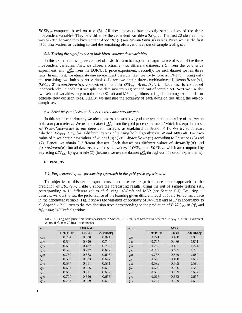
The objective of this set of experiments is to measure the performance of our approach for the

prediction of 𝐵𝑂𝑆𝑉𝐸𝑋𝑇 . Table 3 shows the forecasting results, using the out of sample testing sets,

corresponding to 11 different values of 𝑑 using J48Graft and M5P (see Section 5.1). By using 11

datasets, we want to test the performance of the learning given different level of 𝑇𝑟𝑢𝑒-𝐹𝑎𝑙𝑠𝑒 imbalance

in the dependent variable. Fig. 2 shows the variation of accuracy of J48Graft and M5P in accordance to

𝑑. Appendix B illustrates the two decision trees corresponding to the prediction of 𝐵𝑂𝑆𝑉𝐸𝑋𝑇 in 𝐷45𝐴 and

𝐷25𝐴 using J48Graft algorithm.

Table 3: Using gold price time series described in Section 5.1. Results of forecasting whether 𝑂𝑆𝑉𝐸𝑋𝑇 < 𝑑 for 11 different

values of 𝑑. 𝑛 = 20 in all experiments.

𝒅 = J48Graft

𝒅 = M5P

Precision Recall Accuracy Precision Recall Accuracy

q25 0.704 0.388 0.821 q25 0.741 0.408 0.830

q30 0.500 0.890 0.740 q30 0.727 0.436 0.811

q35 0.620 0.477 0.750 q35 0.718 0.431 0.774

q40 0.530 0.907 0.679 q40 0.738 0.407 0.735

q45 0.780 0.368 0.698 q45 0.733 0.379 0.689

q50 0.589 0.583 0.627 q50 0.615 0.498 0.632

q55 0.574 0.611 0.571 q55 0.592 0.565 0.580

q60 0.684 0.666 0.632 q60 0.609 0.666 0.580

q65 0.638 0.881 0.632 q65 0.633 0.889 0.627

q70 0.700 0.866 0.679 q70 0.663 0.933 0.655

q75 0.704 0.959 0.693 q75 0.704 0.959 0.693

10

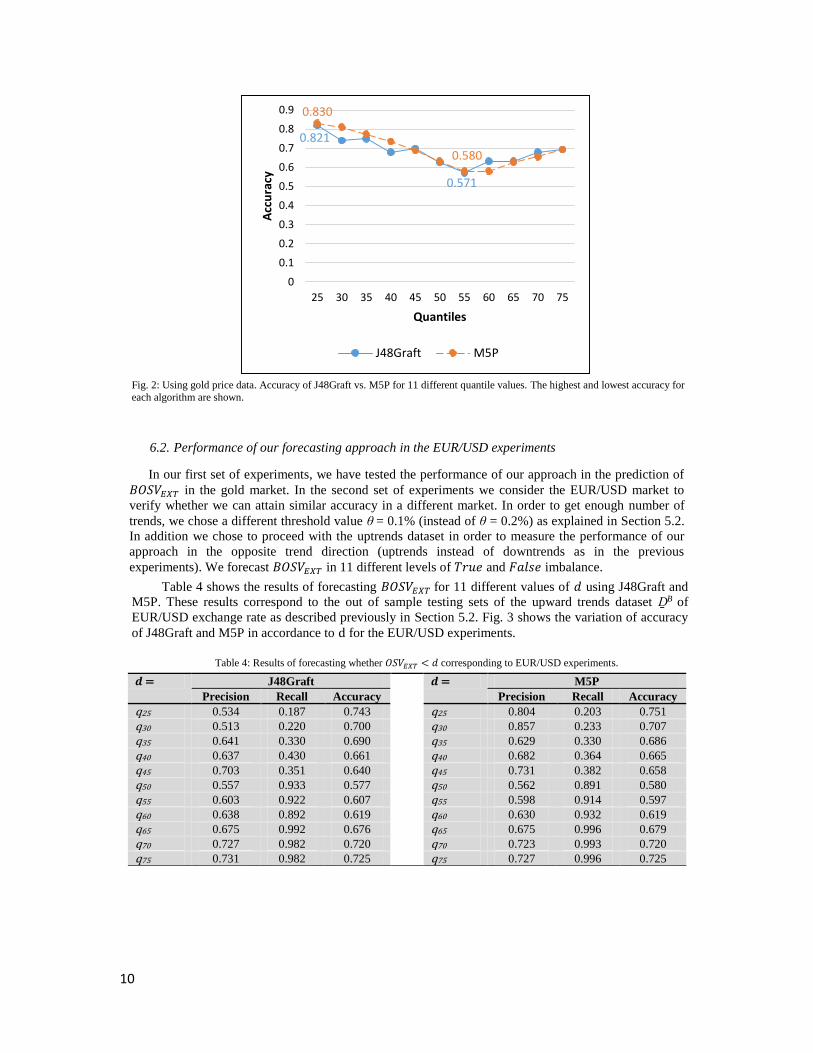
Fig. 2: Using gold price data. Accuracy of J48Graft vs. M5P for 11 different quantile values. The highest and lowest accuracy for

each algorithm are shown.

6.2. Performance of our forecasting approach in the EUR/USD experiments

In our first set of experiments, we have tested the performance of our approach in the prediction of

𝐵𝑂𝑆𝑉𝐸𝑋𝑇 in the gold market. In the second set of experiments we consider the EUR/USD market to

verify whether we can attain similar accuracy in a different market. In order to get enough number of

trends, we chose a different threshold value θ = 0.1% (instead of θ = 0.2%) as explained in Section 5.2.

In addition we chose to proceed with the uptrends dataset in order to measure the performance of our

approach in the opposite trend direction (uptrends instead of downtrends as in the previous

experiments). We forecast 𝐵𝑂𝑆𝑉𝐸𝑋𝑇 in 11 different levels of 𝑇𝑟𝑢𝑒 and 𝐹𝑎𝑙𝑠𝑒 imbalance.

Table 4 shows the results of forecasting 𝐵𝑂𝑆𝑉𝐸𝑋𝑇 for 11 different values of 𝑑 using J48Graft and

M5P. These results correspond to the out of sample testing sets of the upward trends dataset ḎB of

EUR/USD exchange rate as described previously in Section 5.2. Fig. 3 shows the variation of accuracy

of J48Graft and M5P in accordance to d for the EUR/USD experiments.

Table 4: Results of forecasting whether 𝑂𝑆𝑉𝐸𝑋𝑇 < 𝑑 corresponding to EUR/USD experiments.

𝒅 = J48Graft

𝒅 = M5P

Precision Recall Accuracy Precision Recall Accuracy

q25 0.534 0.187 0.743 q25 0.804 0.203 0.751

q30 0.513 0.220 0.700 q30 0.857 0.233 0.707

q35 0.641 0.330 0.690 q35 0.629 0.330 0.686

q40 0.637 0.430 0.661 q40 0.682 0.364 0.665

q45 0.703 0.351 0.640 q45 0.731 0.382 0.658

q50 0.557 0.933 0.577 q50 0.562 0.891 0.580

q55 0.603 0.922 0.607 q55 0.598 0.914 0.597

q60 0.638 0.892 0.619 q60 0.630 0.932 0.619

q65 0.675 0.992 0.676 q65 0.675 0.996 0.679

q70 0.727 0.982 0.720 q70 0.723 0.993 0.720

q75 0.731 0.982 0.725 q75 0.727 0.996 0.725

0.821

0.571

0.830

0.580

0

0.1

0.2

0.3

0.4

0.5

0.6

0.7

0.8

0.9

25 30 35 40 45 50 55 60 65 70 75

Acc

ura

cy

Quantiles

J48Graft M5P

11

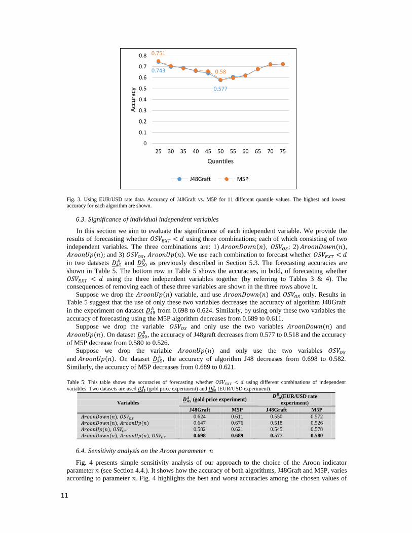
Fig. 3. Using EUR/USD rate data. Accuracy of J48Graft vs. M5P for 11 different quantile values. The highest and lowest

accuracy for each algorithm are shown.

6.3. Significance of individual independent variables

In this section we aim to evaluate the significance of each independent variable. We provide the

results of forecasting whether 𝑂𝑆𝑉𝐸𝑋𝑇 < 𝑑 using three combinations; each of which consisting of two

independent variables. The three combinations are: 1) 𝐴𝑟𝑜𝑜𝑛𝐷𝑜𝑤𝑛(𝑛), 𝑂𝑆𝑉𝑂𝑆; 2) 𝐴𝑟𝑜𝑜𝑛𝐷𝑜𝑤𝑛(𝑛),

𝐴𝑟𝑜𝑜𝑛𝑈𝑝(𝑛); and 3) 𝑂𝑆𝑉𝑂𝑆, 𝐴𝑟𝑜𝑜𝑛𝑈𝑝(𝑛). We use each combination to forecast whether 𝑂𝑆𝑉𝐸𝑋𝑇 < 𝑑

in two datasets 𝐷45𝐴 and 𝐷50

𝐵 as previously described in Section 5.3. The forecasting accuracies are

shown in Table 5. The bottom row in Table 5 shows the accuracies, in bold, of forecasting whether

𝑂𝑆𝑉𝐸𝑋𝑇 < 𝑑 using the three independent variables together (by referring to Tables 3 & 4). The

consequences of removing each of these three variables are shown in the three rows above it.

Suppose we drop the 𝐴𝑟𝑜𝑜𝑛𝑈𝑝(𝑛) variable, and use 𝐴𝑟𝑜𝑜𝑛𝐷𝑜𝑤𝑛(𝑛) and 𝑂𝑆𝑉𝑂𝑆 only. Results in

Table 5 suggest that the use of only these two variables decreases the accuracy of algorithm J48Graft

in the experiment on dataset 𝐷45𝐴 from 0.698 to 0.624. Similarly, by using only these two variables the

accuracy of forecasting using the M5P algorithm decreases from 0.689 to 0.611.

Suppose we drop the variable 𝑂𝑆𝑉𝑂𝑆 and only use the two variables 𝐴𝑟𝑜𝑜𝑛𝐷𝑜𝑤𝑛(𝑛) and

𝐴𝑟𝑜𝑜𝑛𝑈𝑝(𝑛). On dataset 𝐷50𝐵 , the accuracy of J48graft decreases from 0.577 to 0.518 and the accuracy

of M5P decrease from 0.580 to 0.526.

Suppose we drop the variable 𝐴𝑟𝑜𝑜𝑛𝑈𝑝(𝑛) and only use the two variables 𝑂𝑆𝑉𝑂𝑆

and 𝐴𝑟𝑜𝑜𝑛𝑈𝑝(𝑛). On dataset 𝐷45𝐴 , the accuracy of algorithm J48 decreases from 0.698 to 0.582.

Similarly, the accuracy of M5P decreases from 0.689 to 0.621.

Table 5: This table shows the accuracies of forecasting whether 𝑂𝑆𝑉𝐸𝑋𝑇 < 𝑑 using different combinations of independent

variables. Two datasets are used 𝐷45𝐴 (gold price experiment) and 𝐷50

𝐵 (EUR/USD experiment).

Variables 𝑫𝟒𝟓

𝑨 (gold price experiment) 𝑫𝟓𝟎

𝑩 (EUR/USD rate

experiment)

J48Graft M5P J48Graft M5P

𝐴𝑟𝑜𝑜𝑛𝐷𝑜𝑤𝑛(𝑛), 𝑂𝑆𝑉𝑂𝑆 0.624 0.611 0.550 0.572

𝐴𝑟𝑜𝑜𝑛𝐷𝑜𝑤𝑛(𝑛), 𝐴𝑟𝑜𝑜𝑛𝑈𝑝(𝑛) 0.647 0.676 0.518 0.526

𝐴𝑟𝑜𝑜𝑛𝑈𝑝(𝑛), 𝑂𝑆𝑉𝑂𝑆 0.582 0.621 0.545 0.578

𝐴𝑟𝑜𝑜𝑛𝐷𝑜𝑤𝑛(𝑛), 𝐴𝑟𝑜𝑜𝑛𝑈𝑝(𝑛), 𝑂𝑆𝑉𝑂𝑆 0.698 0.689 0.577 0.580

6.4. Sensitivity analysis on the Aroon parameter 𝑛

Fig. 4 presents simple sensitivity analysis of our approach to the choice of the Aroon indicator

parameter 𝑛 (see Section 4.4.). It shows how the accuracy of both algorithms, J48Graft and M5P, varies

according to parameter 𝑛. Fig. 4 highlights the best and worst accuracies among the chosen values of

0.743

0.577

0.751

0.58

0

0.1

0.2

0.3

0.4

0.5

0.6

0.7

0.8

25 30 35 40 45 50 55 60 65 70 75

Acc

ura

cy

Quantiles

J48Graft M5P

12

parameter 𝑛 for each algorithm. For example, the accuracy of M5P decrease by about 16.9% (from

0.632 in case of 𝑛 = 20 to 0.525 in case of = 50 ) and the accuracy of J48Graft decreases by about

17.2% (from 0.627 in case of 𝑛 = 20 to 0.519 in case of 𝑛 = 45).

Fig. 4: Variation of accuracy of forecasting whether 𝑂𝑆𝑉𝐸𝑋𝑇< 𝑑 as function of the Aroon parameter 𝑛 using J48Graft and M5P.

These results correspond to the gold price test-dataset 𝐷50𝐴 . The results corresponding to best and worst accuracy of both

algorithms are presented.

7. DISCUSSION

7.1. Interpretation of the results of gold price experiments

The objective of the gold prices experiments was to test whether our approach can perform better

than random forecast. The accuracy of M5P algorithm in these experiments ranges between 0.580 and

0.830 according to the value of 𝑑 (see Fig. 2). Bear in mind that the investor can choose the value of 𝑑

(see rule (5)). Consequently, the investor can regulate the desired accuracy. Therefore, we consider this

range of accuracy to be acceptable.

In order to compare our results to a random forecast approach, we focus on the results for 𝑑 = q50

(i.e. 50 % of 𝐵𝑂𝑆𝑉𝐸𝑋𝑇 are 𝑇𝑟𝑢𝑒). This is where a random forecast would have an expected accuracy,

precision and recall of 0.500. As can be seen in Table 3 in case of 𝑑 = q50, J48Graft has precision,

recall and accuracy all larger than 0.580, which is better than the performance of random predictions.

The results of gold prices experiments suggest that our approach outperforms random forecasting.

7.2. Comments on EUR/USD experiments’ results

The objective of this set of experiments was to check whether our approach can provide similar

accuracy when applied to another financial market. By comparing Fig. 3 and Fig. 4, we can conclude

that in EUR/USD experiments, we get similar minimum accuracy as in the gold price experiments. The

J48Graft algorithm shows minimum accuracy of 0.577 (case of q50 in Fig. 4) which is very close to the

minimum accuracy obtained using same algorithm in gold price experiments (0.571 in case of q55). The

M5P algorithm show exactly same minimum accuracy of 0.580 in both markets (case of q50 in Fig. 4,

and case of case of q55 in Fig. 3).

However, J48Graft show a maximum accuracy of 0.821 in gold price (in case of q25) comparing to

only 0.743 for same quantile in EUR/USD experiments. The M5P show a maximum accuracy of 0.830

in gold price (in case of q25) comparing to only 0.751 for same quantile in EUR/USD experiments.

Hence we conclude that the obtained accuracies in both set of experiments are, reasonably, similar.

An important note is that the results of EUR/USD experiments, shown in Table 4, were obtained

using same independent variables and same Aroon parameter, 𝑛, value as in the previous experiments.

0.627

0.5190.632

0.525

0

0.1

0.2

0.3

0.4

0.5

0.6

0.7

n10 n15 n20 n25 n30 n35 n40 n45 n50

Acc

ura

cy

Aroon inidcator's paramter 𝑛

forecasting OSVEXT corresponding to quantile d=q50

J48Graft M5P

13

Note also that in these experiments we applied our approach to the uptrends dataset, ḎB, instead of

downtrends dataset, ḎA, as in the first experiment.

7.3. The significance of independent variables

The main challenge is to discover a set of independent variables those are appropriates to the

identified forecasting problem. We have proposed three variables, namely 𝐴𝑟𝑜𝑜𝑛𝑈𝑝(𝑛),

𝐴𝑟𝑜𝑜𝑛𝐷𝑜𝑤𝑛(𝑛) and 𝑂𝑆𝑉𝑂𝑆. The question is: do all these variables contribute to the success of our

forecast? To answer this question, we refer to Table 5 in Section 6.3, which presented the results of

omitting each of the variables. In this section, we examine the results of omitting each of the variables

with the results of using all the three variables.

The results highlighted in Section 6.3 suggests performance decreases if we drop any of the three

independent variables. This shows that each of the independents variables contributes significantly to

our forecasting task.

7.4. Sensitivity analysis of the Aroon indicator’s parameter 𝑛.

To analyze the sensitivity of our approach to the parameter 𝑛 (see Equations (6) and (7)), we try to

forecast 𝐵𝑂𝑆𝑉𝐸𝑋𝑇 in 𝐷50𝐴 using 9 different values of parameter 𝑛 as explained in Section 4.4 based on

Fig. 4, the accuracy of both algorithms decreases significantly, by 16.9% for M5P and 17.2% for

J48Graft, from one value of 𝑛 to another (see Section 6.4). Hence, this test provides evidence that our

approach is sensitive to the parameter 𝑛. A general deduction is that if we want to apply our approach to

another time series than gold price, then we should first conduct the sensitivity analysis to 𝑛.

7.5. Analysis summary

The results of both experiments show that our approach outperform random forecasting. Both

experiments provide comparable results using same parameters’ values (even though we have used two

different thresholds and different trends’ datasets). Therefore, we believe that our approach can be

applied to other time series. The parameter 𝑑 is essential to develop a trading strategy in a later

research. Table 5 provide evidence that each independent variable is an important part of our approach.

Based on Fig. 4, we conclude that our forecasting approach could be sensitive to the Aroon indicator’s

parameter 𝑛.

8. CONCLUSION

Directional change (DC) is a new, data-driven framework that aims to record significant price

changes. In a DC-based summary, the market is cast into alternating upward and downward trends. In

an upward trend, we say that the trend has changed (into a downward trend) if price has dropped from

the highest point in the current trend by a certain threshold (e.g. 1%). That means we only know that the

trend has changed in hindsight. Clearly, it will be useful if one could forecast how far the current trend

will continue before the trend changes. This paper presents to first attempt towards this forecasting

problem.

The first contribution of this paper is in formulating a forecasting problem in the context of DC. We

have defined the Boolean variable 𝐵𝑂𝑆𝑉𝐸𝑋𝑇 , which indicates whether the overshoot value at the next

extreme, 𝑂𝑆𝑉𝐸𝑋𝑇 , will exceed a predefined value d. The objective is to predict whether 𝐵𝑂𝑆𝑉𝐸𝑋𝑇 is true

or false. In other words, we want to forecast the next extreme price, i.e. price at which the trend

reverses.

Our second contribution is identifying three independent variables, and proving that they are

relevant to the prediction of 𝑂𝑆𝑉𝐸𝑋𝑇 . The independent variables are: 𝑂𝑆𝑉𝑂𝑆, 𝐴𝑟𝑜𝑜𝑛𝑈𝑝(𝑛) and

𝐴𝑟𝑜𝑜𝑛𝐷𝑜𝑤𝑛(𝑛). We have adapted the Aroon variables from the literature to suit the DC framework. In

order to prove that the identified independent variables are relevant to the prediction of 𝑂𝑆𝑉𝐸𝑋𝑇 , we

have applied them in two forecasting algorithms and conducted four sets of experiments.

14

Our first set of experiments was conducted using minute-by-minute gold price. The aim was to

provide basic assessment of our approach. Results of the experiments show that our approach

outperforms random forecasting in term of accuracy. It turns out that our approach can perform pretty

well (showing minimum accuracy of 0.580) for different selected value of 𝑂𝑆𝑉𝐸𝑋𝑇; it achieved

remarkable results (with accuracy up to 0.830) in some cases.

Our second set of experiments used minute-by-minute EUR/USD exchange rate. The aim was to test

whether our results in the gold market was a one-off. Therefore, we kept the same parameter values that

we used for the first set of experiments. The performance of our approach in the EUR/USD market was

as good as its performance in the gold market. The results of this experiment suggest that performance

of our approach in the gold market was not a one-off. The obtained results suggest that the independent

variables are also relevant to the EUR/USD market.

In the third set of experiments, we show that each of the three independent variables is important to

our approach. We showed that performance deteriorated if we eliminate any of the three variables in the

forecast.

The final set of experiments showed that the results obtained using our approach can be sensitive to

the choice of Aroon indicator parameter 𝑛. The accuracy may decrease by more than 16% for different

values of 𝑛.

To summarize, this is the first attempt to forecast directional changes under the DC-framework. Our

contribution is in formulating the forecasting problem, identifying a set of independent variables and

proving that they are relevant to the forecasting task. Having established the predictive power of our

approach, our next goal will be to embed this forecasting result into trading strategies.

References

Ao, H., & Tsang, E. (2013). Capturing Market Movements with Directional Changes. Working Paper WP069-13,

Centre for Computational Finance and Economic Agents (CCFEA). Colechester, UK: University of Essex.

Baron, M., Brogaard, J., & Kirilenk, A. (2014). Risk and Return in High Frequency Trading. . U.S.: Commodity

Futures Trading Commission (CFTC).

Bisig, T., Dupuis, A., Impagliazzo, V., & Olsen, R. (2012). The scale of market quake. Quantitative Finance, 12(4),

501-508.

Chande, T., & Kroll, S. (1994). The new technical trader. New York, USA: John Wiley and Sons.

Das, S., & Padhy, S. (2012). Support Vector Machines for Prediction of Futures Prices in Indian Stock Market.

International Journal of computer Application, 41(3), 22-26.

Dupuis, A., & Olsen, R. (2012). High Frequency Finance: Using Scaling Laws to Build Trading Models. In J. James et

al (Ed.), Handbook of Exchange Rates (pp. 563-582). NJ,USA: Wiley.

Ehlers, J. (2002). MESA and Trading Market Cycles: Forecasting and Trading Strategies from the Creator of MESA.

New York, USA: John Wiley & Sons.

Glattfelder, J., Dupuis, A., & Olsen, R. (2011). Patterns in high-frequency FX data: Discovery of 12 empirical scaling

laws. Quantitative Finance, 11(4), 599-614.

Guillaume, D., Dacorogna, M., Davé, R., Müller, U., Olsen, R., & Pictet, O. (1997). From the bird's eye to the

microscope: A survey of new stylized facts of the intra-daily foreign exchange markets. Finance and

stochastic, 1(2), 95-129.

Hassan, M. (2009). A combination of hidden Markov model and fuzzy model for stock market forecasting.

Neurocomputing, 16(92), 3439-3446.

Hassan, M., & Nath, B. (2005). Stock Market Forecasting Using Hidden Markov Model: A New Approach.

International Conference on Intellignet System Design and Application (pp. 192-196). Wroclaw, Poland:

IEEE.

15

Iqbal, Z., Ilyas, R., Shahzad, W., Mahmood, Z., & Anjum, J. (2013). Efficient Machine Learning Techniques for Stock.

International Journal of Engineering Research and Applications, 3(6), 855-867.

Jin, N., Tsang, E., & Li, J. (2009). A constraint-guided method with evolutionary algorithms for economic problems.

Applied Soft Computing Journal, 9(3), 924-935.

Kokare, A., Venkatesan, P., Tandel, S., & Palivela, H. (2014). Survey On Classification Based Techniques On Non-

Spatial Data. International Journal of Innovative Research in Science, Engineering and Technology, 3(1),

409-413.

Masry, S. (2013). Event-Based Microscopic Analysis of the FX Market. PhD thesis, Centre for Computational Finance

and Economic Agents (CCFEA). Colchester: University of Essex.

Park, S.-H., Lee, J.-H., Song, J.-W., & Park, T.-S. (2009). Forecasting Change Directions for Financial Time Series

Using Hidden Markov Model. In P. Wem et al (Ed.), 4th ROUGH SETS AND KNOWLEDGE

TECHNOLOGY. RSKT 2009, LNCS 5589, pp. 184-191. Gold Coast: Springer-Verlag, Berlin.

Quinlan, J. (1992). Learning with continuous classes. 5th Australian Joint Conference on Artificial Intelligence (pp.

343-348). Singapore: World Scientific.

Quinlan, J. (1993). C4.5: Programs for Machine Learning. San Francisco, CA,USA: Morgan Kaufmann Publishers Inc.

Rajput, S., & Arora, A. (2013). Designing Spam Model- Classification Analysis using Decision Trees. International

Journal of Computer Applications, 75(10), 6-12.

Skabar, A. (2008). Direction-of-Change Financial Time Series Forecasting using Bayesian Learning for MLPs.

Proceedings of the World Congress on Engineering. II, pp. 1160-1165. London, UK.: the World Congress on

Engineering.

Tsang, E. (2010). Directional Changes, Definition. Working Paper WP050-10, Center of Computational Finance and

Economic Agent (CCFEA). Colchester: university of Essex.

Tsang, E., & Garcia-Almanza, A. (2011). Evolutionary Applications for Financial Prediction: Classification Methods

to Gather Patterns Using Genetic Programming. VDM Verlag Dr. Müller.

Tsang, E., & Li, J. (2002). EDDIE for financial forecasting. In S.-H. Chen (Ed.), Genetic Algorithms and Programming

in Computational Finance (pp. 161-174). Kluwer Series in computational finance.

Wang, J.-H., & Leu, J.-Y. (1996). Stock market trend prediction using ARIMA-based neural networks. International

Conference on Neural Networks. 4, pp. 2160-2165. Washington DC, USA: IEEE.

Wang, Y., & Witten, I. (1997). Induction of model trees for predicting continuous classes. In M. Van Someren, & G.

Widmer, Lecture Notes in Computer Science (pp. 128-137). Berlin: Springer.

Webb, G. (1999). Decision tree grafting from the all-tests-but-one partition. International Joint Conference on

Artificial Intelligence. 2, pp. 702-707. San Francisco, CA,: Morgan Kaufmann Publishers Inc.

White, H. (1988). Economic prediction using Neural Networks: The case of IBM daily stock returns. International

Conference on Neural Networks. 2, pp. 451-458. CA, USA: IEEE.

Wilder, J. W. (1978). New Concepts in Technical Trading Systems. McLeansville, N.C., USA: Hunter Publishing

Company.

Witten, H., Frank, E., & Hall, M. A. (2011). Data Mining Practical Machine Learning Tools and Techniques, Third

Edition. Burlington, USA: Elsevier Inc.

Yang, K., Wu, M., & Lin, J. (2012). The application of fuzzy neural networks in stock price forecasting based On

Genetic Algorithm discovering fuzzy rules. International Conference on Natural Computation (pp. 470-474).

Beijing, China: IEEE.

16

Appendix A: Pseudo-code to compute the variables defined in Section 3

In this appendix, we present the pseudo code of a procedure that finds all the directional changes in

a series. The following procedure DCBasedAnalysis takes 2 parameters as input: the price time series ts

and the threshold 𝜃 related to the DC concept as explained previously in Section 1. This procedure

return a matrix DCBasedAnalysis which is composed of 3 numerical vectors: 𝑃𝐸𝑋𝑇; 𝑂𝑆𝑉𝑂𝑆 and 𝑂𝑆𝑉𝐸𝑋𝑇 . Each row in DCBasedAnalysis represents one trend.

The following variables are used in the procedure DCBasedAnalysis below:

𝑃𝐸𝑋𝑇𝑖 : The price extreme at which the ith trend starts. The vector 𝑃𝐸𝑋𝑇 contains all computed

𝑃𝐸𝑋𝑇𝑖 . 𝑂𝑆𝑉𝑂𝑆

𝑖 : The overshoot value computed at ith DC confirmation point as explained in Table1. The

vector 𝑂𝑆𝑉𝑂𝑆 contains all computed 𝑂𝑆𝑉𝑂𝑆𝑖 .

𝑂𝑆𝑉𝐸𝑋𝑇𝑖 : The overshoot value computed at the start of next trend as explained in Table 2. The

vector 𝑂𝑆𝑉𝐸𝑋𝑇 contains all computed 𝑂𝑆𝑉𝐸𝑋𝑇𝑖 .

𝑃𝑐 records the price currently being processed.

The variable mode records the current mode, which is initialized to up.

𝑃𝐷𝐶𝐶∗𝑖 is the target price for directional change confirmation corresponding to the ith trend (under

threshold θ).

Procedure DCBasedAnalysis (time series ts, threshold 𝜃)

Initialize variables: Pc =PEXT = ts [1] = price of first observation, mode = up, 𝑃𝐷𝐶𝐶∗𝑖 = 𝑃𝑐 × (1+ 𝜃)

Len = number of observations in ts i=2 Loop until i=Len Pc =ts[i] if mode = down then if Pc < 𝑃𝐸𝑋𝑇

𝑖+1 then 𝑃𝐸𝑋𝑇

𝑖+1 = Pc else if (Pc −𝑃𝐸𝑋𝑇

𝑖+1 ) ÷ 𝑃𝐸𝑋𝑇𝑖+1 ≥ 𝜃 then

𝑂𝑆𝑉𝐸𝑋𝑇𝑖 = ((𝑃𝐸𝑋𝑇

𝑖 – 𝑃𝐷𝐶𝐶∗𝑖 ) ÷ 𝑃𝐷𝐶𝐶∗

𝑖 ) ÷ θ

𝑃𝐷𝐶𝐶∗𝑖+1 = 𝑃𝐸𝑋𝑇

𝑖+1 × (1- θ)

𝑂𝑆𝑉𝑂𝑆𝑖+1 = ((Pc – 𝑃𝐷𝐶𝐶∗

𝑖+1 ) ÷ 𝑃𝐷𝐶𝐶∗𝑖+1 ) ÷ θ

𝑃𝐸𝑋𝑇𝑖+1 = Pc

mode = up end if else if mode = up then if Pc > 𝑃𝐸𝑋𝑇

𝑖+1 then 𝑃𝐸𝑋𝑇

𝑖+1 = Pc else if (Pc −𝑃𝐸𝑋𝑇

𝑖+1 ) ÷ 𝑃𝐸𝑋𝑇𝑖+1 ≤ − 𝜃 then

𝑂𝑆𝑉𝐸𝑋𝑇𝑖 = ((𝑃𝐸𝑋𝑇

𝑖 – 𝑃𝐷𝐶𝐶∗𝑖 ) ÷ 𝑃𝐷𝐶𝐶∗

𝑖 ) ÷ θ

𝑃𝐷𝐶𝐶∗𝑖+1 = 𝑃𝐸𝑋𝑇

𝑖+1 × (1+ θ)

𝑂𝑆𝑉𝑂𝑆𝑖+1 = ((Pc – 𝑃𝐷𝐶𝐶∗

𝑖+1 ) ÷ 𝑃𝐷𝐶𝐶∗𝑖+1 ) ÷ θ

𝑃𝐸𝑋𝑇𝑖+1 =Pc

mode = down end if end if i=i+1 End Loop

DCAnalysis = as.matrix (𝑃𝐸𝑋𝑇; 𝑂𝑆𝑉𝑂𝑆; 𝑂𝑆𝑉𝐸𝑋𝑇) Return DCAnalysis

17

Appendix B: Two samples decision trees based on gold prices experiments.

Below we illustrate two decision trees. Each decision tree is associated with an interpretation in

form of if- else rules. Fig. B.1 illustrates the decision tree corresponding to the prediction of 𝐵𝑂𝑆𝑉𝐸𝑋𝑇

for dataset 𝐷25𝐴 using J48Graft algorithm. Fig. B.2 illustrates the decision tree corresponding to the

prediction of 𝐵𝑂𝑆𝑉𝐸𝑋𝑇 for dataset 𝐷45𝐴 using J48Graft algorithm.

Fig. B.1. The decision tree generated by J48Graft algorithm to forecast whether 𝑩𝑶𝑺𝑽𝑬𝑿𝑻 based on the gold price dataset 𝑫𝟐𝟓𝑨 (see

Section 5.1 for explanation). The black nodes (i.e. true and false nodes) refer to the forecasted value of whether 𝑩𝑶𝑺𝑽𝑬𝑿𝑻. Each blue node presents an if-condition. When the if-condition is true, we proceed with the right child node (i.e. the one corresponding to

the green edge); otherwise we proceed the left child node (i.e. the one corresponding to the red edge).

Fig. B.2. The decision tree generated by J48Graft algorithm to forecast whether 𝑶𝑺𝑽𝑬𝑿𝑻 < 𝒅 based on the gold price dataset 𝑫𝟒𝟓𝑨 .

The black nodes (i.e. true and false nodes) refer to the forecasted value of whether 𝑶𝑺𝑽𝑬𝑿𝑻 < 𝒅. Each blue node presents an if-condition. When the formulated if-condition is true, we proceed with the right child node (i.e. the one corresponding to the green

edge); otherwise we proceed the left child node (i.e. the one corresponding to the red edge).

if 𝐴𝑟𝑜𝑜𝑛𝐷𝑜𝑤𝑛≤ 95

if 𝐴𝑟𝑜𝑜𝑛𝑈𝑝≤ 97.5

False True

if 𝐴𝑟𝑜𝑜𝑛𝐷𝑜𝑤𝑛 ≤ 70

if 𝑂𝑆𝑉𝑂𝑆

≤ −0.676517

Falseif 𝑂𝑆𝑉𝑂𝑆

≤ −1.660892

if 𝐴𝑟𝑜𝑜𝑛𝐷𝑜𝑤𝑛 ≤ 85

False if 𝐴𝑟𝑜𝑜𝑛𝑈𝑝 ≤ 5

if 𝐴𝑟𝑜𝑜𝑛𝐷𝑜𝑤𝑛 ≤ 30

if 𝑂𝑆𝑉𝑂𝑆

≤ −0.705356

True False

True

False

True

False

if 𝐴𝑟𝑜𝑜𝑛𝐷𝑜𝑤𝑛 ≤ 95

True if 𝑂𝑆𝑉𝑂𝑆 ≤ −0.958299

if 𝐴𝑟𝑜𝑜𝑛𝑈𝑝 ≤ 95

if 𝑂𝑆𝑉𝑂𝑆≤ −0.321513

Flase True

if 𝐴𝑟𝑜𝑜𝑛𝑈𝑝 ≤ 90

if 𝐴𝑟𝑜𝑜𝑛𝐷𝑜𝑤𝑛 ≤ 92.5

False True

False

True

false

false true

Interpretation of this decision tree:

if 𝐴𝑟𝑜𝑜𝑛𝐷𝑜𝑤𝑛 ≤ 95

| if 𝑂𝑆𝑉𝑂𝑆 ≤ −0.958299: True | else

| | if 𝐴𝑟𝑜𝑜𝑛𝑈𝑝 ≤ 95

| | | if 𝐴𝑟𝑜𝑜𝑛𝑈𝑝 ≤ 90: False | | | else

| | | | if 𝐴𝑟𝑜𝑜𝑛𝐷𝑜𝑤𝑛 ≤ 92.5: True | | | | else: False

| | else

| | | if 𝑂𝑆𝑉𝑂𝑆 ≤ −0.321513: True

| | | else: False

else: True

Interpretation of this decision tree:

if 𝐴𝑟𝑜𝑜𝑛𝐷𝑜𝑤𝑛 ≤ 95

| if 𝐴𝑟𝑜𝑜𝑛𝐷𝑜𝑤𝑛 ≤ 70: False

| else

| | if 𝑂𝑆𝑉𝑂𝑆 ≤ −0.676517

| | | if 𝑂𝑆𝑉𝑂𝑆 ≤ −1.660892: True

| | | else

| | | | if 𝐴𝑟𝑜𝑜𝑛𝐷𝑜𝑤𝑛 ≤ 85

| | | | | if 𝐴𝑟𝑜𝑜𝑛𝑈𝑝 ≤ 5: False

| | | | | else

| | | | | | if 𝐴𝑟𝑜𝑜𝑛𝐷𝑜𝑤𝑛 ≤ 30: True | | | | | | else

| | | | | | | if 𝑂𝑆𝑉𝑂𝑆 ≤ −0.705356: False | | | | | | | else: True

| | | | else: False

| | else: False else

| | if 𝐴𝑟𝑜𝑜𝑛𝑈𝑝 ≤ 97.5: True

| else: False

true