fluvial sediment transport: analytical techniques for measuring

IAEA-TECDOC-1461

Fluvial sediment transport: Analytical techniques for measuring sediment load

July 2005

The originating Section of this publication in the IAEA was:

Isotope Hydrology Section International Atomic Energy Agency

Wagramer Strasse 5 P.O. Box 100

A-1400 Vienna, Austria

FLUVIAL SEDIMENT TRANSPORT: ANALYTICAL TECHNIQUES FOR MEASURING SEDIMENT LOAD

IAEA, VIENNA, 2005 IAEA-TECDOC-1461 ISBN 92–0–107605–3

ISSN 1011–4289 © IAEA, 2005

Printed by the IAEA in Austria July 2005

FOREWORD

The IAEA supported its first technical cooperation project on the study of sediment transport using nuclear techniques in the early 1970s. Since 1976, more than 28 projects on this topic were successfully completed with the assistance of the IAEA, allowing the countries of Asia, Africa and Latin America to improve the management of dam reservoirs, harbours, canals and rivers. Due to the importance of understanding sediment transport, measurement techniques are continuously being improved and innovative non-nuclear techniques have become more competitive. Therefore, an updated overview of the techniques used today for evaluation of sediment transport in rivers was considered to be necessary. Users from Member States would then be able to select a suitable technique for their specific problems, knowing the technical and economic limitations and advantages of the nuclear and non-nuclear techniques.

In 2003 a group of experts was invited to a consultants meeting on the preparation of a report on river sediment transport studies. The objective of the meeting was to prepare a short publication that would include the general principles of sediment transport, a description of the classical method and the principles, advantages/limitations and future development of the continuous measurement techniques such as acoustical, laser and nuclear. The report would be concise and usable for the general public.

This report does not give an extensive review of the techniques used for the measurement of suspended and bed load sediment transport in rivers. It is a guidebook to help water managers define the appropriate techniques to be used for their specific study, taking into account the available resources and natural physical conditions of the river and sediment transport. This report will help the IAEA give adequate support to the TC counterparts to solve their specific problems related to transport of sediment in rivers.

The publication was prepared in collaboration with P. Brisset (France), G. Old (United Kingdom) and D. Wren (USA). The IAEA greatly appreciates the assistance of T. Melis of the United States Geological Survey (USA) for his support related to the use of acoustic techniques. The IAEA officer responsible for this publication was L. Gourcy of the Division of Physical and Chemical Sciences.

EDITORIAL NOTE

The use of particular designations of countries or territories does not imply any judgement by the publisher, the IAEA, as to the legal status of such countries or territories, of their authorities and institutions or of the delimitation of their boundaries.

The mention of names of specific companies or products (whether or not indicated as registered) does not imply any intention to infringe proprietary rights, nor should it be construed as an endorsement or recommendation on the part of the IAEA.

CONTENTS

SUMMARY ............................................................................................................................... 1

1. INTRODUCTION ............................................................................................................ 5

1.1. Scope of the report.............................................................................................. 5 1.2. Methods presented .............................................................................................. 5

2. TECHNIQUES FOR MEASURING SUSPENDED SEDIMENT (CURRENTLY AVAILABLE) .................................................................................................................. 7

2.1. Directly sampling water/sediment mixture......................................................... 7 2.1.1. Grab sample ............................................................................................ 7 2.1.2. Pump sampling ....................................................................................... 8 2.1.3. Isokinetic sampling ................................................................................. 9 2.1.4. Sample analysis..................................................................................... 11

2.2. Optical .............................................................................................................. 14 2.2.1. Scattering .............................................................................................. 14 2.2.2. Transmission......................................................................................... 16

2.3. Nuclear.............................................................................................................. 17 2.3.1. Scattering .............................................................................................. 17 2.3.2. Transmission......................................................................................... 21

2.4. Acoustic (single frequency).............................................................................. 27 2.4.1. Operating principle ............................................................................... 27 2.4.2. Application guidelines .......................................................................... 28

2.5. Laser diffraction ............................................................................................... 30 2.5.1. Operating principle ............................................................................... 30 2.5.2. Application guidelines .......................................................................... 31

2.6. Tracer techniques.............................................................................................. 32 2.6.1. Operating principle ............................................................................... 32 2.6.2. Application guidelines .......................................................................... 35

3. TECHNIQUES FOR MEASURING SUSPENDED SEDIMENT (UNDER DEVELOPMENT).......................................................................................................... 36

3.1. Acoustic (multiple frequency) .......................................................................... 36 3.2. Pressure differential .......................................................................................... 36 3.3. Digital imaging ................................................................................................. 37

4. TECHNIQUES FOR MEASURING BEDLOAD (CURRENTLY AVAILABLE) ...... 37

4.1. The pressure-difference type samplers ............................................................. 37 4.1.1. Operating principle ............................................................................... 37 4.1.2. Application guidelines .......................................................................... 39

4.2. Portable bedload traps ...................................................................................... 39 4.2.1. Operating principle ............................................................................... 40 4.2.2. Application guidelines .......................................................................... 41

4.3. Permanent traps ................................................................................................ 41 4.3.1. Operating principle ............................................................................... 41 4.3.2. Application guidelines .......................................................................... 42

4.4. Nuclear gauges ................................................................................................. 43 4.4.1. Operating principle ............................................................................... 43 4.4.2. Application guidelines .......................................................................... 44

4.5. Tracer techniques.............................................................................................. 44 4.5.1. Operating principle ............................................................................... 44 4.5.2. Application guidelines .......................................................................... 46

5. TECHNIQUES FOR MEASURING BEDLOAD (UNDER DEVELOPMENT).......... 49

5.1. Passive acoustic ................................................................................................ 49 5.2. Sonar imaging................................................................................................... 49 5.3. Impact sensors .................................................................................................. 49

6. CONCLUSIONS ............................................................................................................ 50

REFERENCES......................................................................................................................... 53

BIBLIOGRAPHY .................................................................................................................... 57

CONTRIBUTORS TO DRAFTING AND REVIEW ............................................................. 61

1

SUMMARY

Studies of sediment transport are important for many projects and are highly complex. The projects may include river and marine engineering problems such as dam construction and management which involve direct interference with the water to land or bed boundary, or environmental projects such as deforestation programmes which may affect catchment erosion rates and thus give rise to sedimentation problems in rivers and lakes.

Major concerns for engineers, hydrologists and environmentalists include (i) the maintenance and planning of future navigable channels; (ii) optimizing dredging practice; (iii) assisting the design of harbour inlet by-passing schemes; (iv) reduction of the effective life of man-made lakes behind power barrage or reservoir dams by sedimentation; (v) channel degradation and (vi) elimination of sediment from irrigation networks.

The input data requested for such studies is flow and bed characteristics and the quantity of sediment in motion. This includes evaluation of sediment yield with respect to different natural environmental conditions, time distribution of sediment concentration and transport rate in streams, evaluation of deposition in channel systems, amount and size characteristics of sediment delivered to a body of water, and sediment particle size distribution.

Universal equations were developed to predict the amount and characteristics of sediment transport and deposition. However, equations cannot predict many aspects of sedimentation and complementary measurements are absolutely necessary. The complex phenomena of fluvial sedimentation cause the required measurements and related analyses of sediment data to be relatively expensive in comparison to other hydrological data. Various measurement methods exist and should be selected based on the size of the river, the scope of the project, the type of sediment transported, the material available locally, national regulations.

The publication presents the methods used today for evaluation of sediment transport in rivers and gives a short overview of the methods under development. The objective is to help in selecting the most appropriate method for a given study.

The first method developed is the manual sampling of suspended sediment and analyses of the characteristics of the material collected. In the mid-1800s, flow from the Mississippi River was first sampled for sediment discharge. Between 1925 and 1940, in order to gather data for an increasing number of sediment studies, investigators developed new sediment samplers to measure fluvial sediment. In 1939, The United States Government organized an interagency program to study methods and equipment used in measuring sediment discharge and to improve and standardize equipment and methods. This organization, called the Federal Interagency Sedimentation Project (FISP), is an important resource, particularly in the area of the manual sampling methodology (http://fisp.wes.army.mil/). Manual sediment sampling is highly time-consuming and cumbersome but is reliable and accurate and remains a reference (and so used for calibration of other methods) as it is the most widely and often used and allows the determination of the size distribution. The sampling can be done manually (grab sample) or using a pump. Isokinetic samplers are divided into depth- and point-integrated categories.

The other instrumented techniques permit data recording in real time. The gauges and sensors measure turbidity, time of reflection of a laser incident on sediment particles, backscatter of

1

2

high frequency sound incident on particles, or transmission of gamma or X rays, refraction angle of a laser incident on particles, backscatter or transmission of visible or infrared light, light reflected and scattered from body of water. This equipment must be calibrated in order to convert raw data into total sediment transport. Acoustic, laser diffraction, optical backscatter and transmission, and nuclear techniques have advantages and disadvantages and in many cases more than one technique should be used in order to obtain reliable information.

Optical methods offer two possibilities: scattering and transmission. Transmission systems were developed for determining total suspended matter or turbidity in marine environment. They show minimum disturbance to flow but require frequent calibration using the sediment present in the area. Diatoms, algae, and organic detritus cause turbidity in the water column, as they cannot be distinguished from suspended sediment. The sensors are very sensitive to biological fouling. Optical backscatter sensors (OBSs) response to varying concentrations of homogeneous sediments is nearly linear. The sensors allow good spatial and temporal resolution. Its design is simple, compact and capable of measuring much higher particle concentrations than a transmissometer, though they lack the accuracy of the transmissometer at low-particle concentrations. Optical sensors are more sensitive to small particles than acoustic methods.

The nuclear techniques include the use of probes (scattering and transmission principle) and artificial radioactive tracers. Since the 1950s certain nuclear techniques have been developed for sediment transport and sedimentation problems. Nuclear techniques have played a major role in recent years notably in the use of radiation probes for measuring very high densities of suspended sediment, such as during dam flushing. The method is well suited to installations where continuous monitoring is necessary and can be used for a wide range of sediment concentration. Low sensitivity is a major limitation as well as the need for licensing and training for using nuclear devises. The nuclear tracers generally used are gamma emitters. The choice of tracers depends on the duration of experiment and nature of the sediment. Tracers are not used for the determination of the suspended sediment concentration but for measuring dynamics of the sediment in a flow. This data is indispensable to study sediment release from dam flushing, wastewater treatment plants, and dredging operations.

Acoustic single frequency sensors permit to quantitatively estimate suspended sediment concentration from acoustic backscatter intensity. At the early 1980’s, the method provided only qualitative results. The first quantitative data was obtained 10 years later. The method is non-intrusive and overcomes the problem of biological fouling. One of the limitations is that it cannot differentiate between changes in concentration and changes in particle size distribution. Acoustic sensors are more sensitive to large particles than optical methods.

Recently, laser instrumentation has been developed that provides an alternative for measuring in situ suspended sediment. A well-known, commercially available laser sensor is the Laser In Situ Scattering and Transmissometer (LISST). It measures the scattering of a laser beam by particles in a volume of water. Sensors are small and suitable for field deployment with real-time data return capabilities. The instrument is powerful for low concentration determination but is quite expensive and susceptible to biological fouling. Acoustic multiple frequency, pressure differential and digital imaging are some of the more promising methods under development. Bed-load transport is even more difficult to estimate in alluvial streams than suspended sediment and poses a particular problem in high-energy bedrock rivers. So far, no sediment-

2

3

monitoring agencies have been able to devise a standard sampler that can be used without elaborate field calibration or that can be used under a wide range of bedload conditions. The samplers used are giving quite different results depending on river characteristics so a combination of sampling methods should be used. The pressure-difference samplers are the most widely used devices for obtaining estimates of bedload transport in natural stream systems. The overall sampling efficiency of a specific sampler is not constant, but varies with size distributions, stream velocities near the bed, turbulence, rate of bed-load transport, and the degree of filling of the sampler. The sampler is portable and can be used in small or rivers however it is not easy to use at high flows. Sampling procedures are highly labour intensive and therefore are quite expensive. The use of different sampler types is recommended. Portable bedload traps are best at relatively low flows and should be better installed at a wide riffle. Various traps should be used. Portable trap operation is limited to flows in which an operator can reach down to the stream bottom to empty the traps. The traps are not suitable for collecting particles smaller than 4 mm. Portable traps are easy to operate at moderately high flows.

Various systems of permanent traps have been developed. Some examples are; the conveyor belt slot system, the Vortex tube system, the weighing slot (pit) sampler system, and the Birkbeck-type automatic monitoring slot sampler. Substantial streambed construction is involved in their installation, making these devices difficult, time consuming and costly to deploy. This method allows a continuous and automatic bedload transport measurement often under-predict transport rates at high flows. The technique is usually used in perennial or seasonal streams when the flow is predictable. The nuclear scattering and transmission system can be used for bedload transport determination. The transmission system is the simpler and more sensitive of the two. Nuclear techniques have played a major role for determination of bed-load transport thanks to the use of artificial radioactive tracers. Pebbles are individually labeled with radionuclides. The results obtained are the direction of the sediment motion, the average speed of its movement, the thickness of the moving layer, and the sediment load. The technique is applicable in any situation where the user has safe access to the water and where a boat is suitable for the local conditions. The use of ionizing radiation requires a clearance from local authorities and specific training.

Passive acoustic, sonar imaging and impact sensors techniques are being developed for a more accurate and less costly measurement of bedload transport.

The methods for suspended sediment study are covered in more details than for bedload. The bibliography given will allow the lecturer to complete the information and know more about field deployment and the techniques themselves.

A consistent approach to estimating transport is not just a matter of which formula or sampler to use; a suitable approach requires a consistent and reliable scaling of water discharge and an integral description of the sediment that is meaningful and practical. This is beyond the scope of this publication.

3

5

1. INTRODUCTION

1.1. Scope of the report

The transport of sediment particles in rivers has important implications for the management of drainage basins and coastal areas. Sediment transport data are often used for the evaluation of land surface erosion, reservoir sedimentation, ecological habitat quality and coastal sediment budgets. Sediment transport by rivers is usually considered to occur in two major ways: (1) in the flow as suspended load and (2) along the bed as bedload. This publication provides guidance on selected techniques for the measurement of particles moving in both modes in the fluvial environment. The relative importance of the transport mode is variable and depends on the hydraulic and sedimentary conditions. The potential user is directed in the selection of an appropriate technique through the presentation of operating principles, application guidelines and estimated costs. A distinction is made between techniques that are currently available and those that are under development. The interpretation of sediment transport data, the standard sampling procedures and the study of the sediment quality are beyond the scope of this document.

1.2. Methods presented

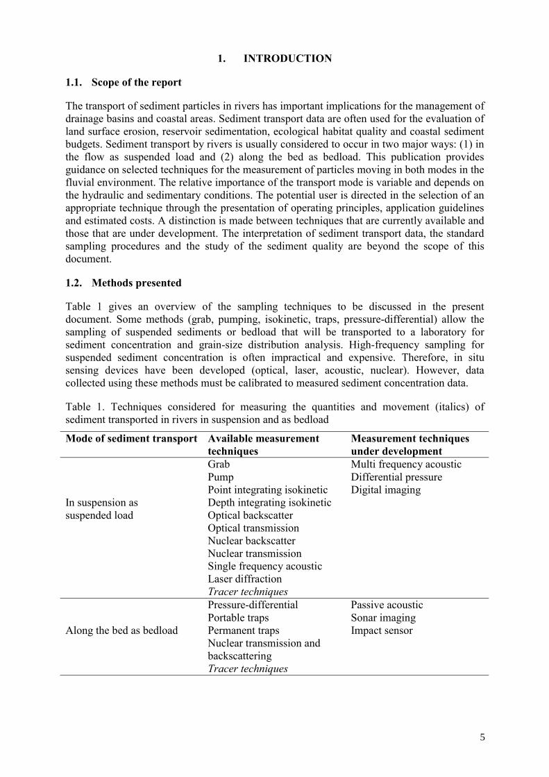
Table 1 gives an overview of the sampling techniques to be discussed in the present document. Some methods (grab, pumping, isokinetic, traps, pressure-differential) allow the sampling of suspended sediments or bedload that will be transported to a laboratory for sediment concentration and grain-size distribution analysis. High-frequency sampling for suspended sediment concentration is often impractical and expensive. Therefore, in situ sensing devices have been developed (optical, laser, acoustic, nuclear). However, data collected using these methods must be calibrated to measured sediment concentration data.

Table 1. Techniques considered for measuring the quantities and movement (italics) of sediment transported in rivers in suspension and as bedload

Mode of sediment transport Available measurement techniques

Measurement techniques under development

Grab Multi frequency acoustic Pump Differential pressure Point integrating isokinetic Digital imaging In suspension as Depth integrating isokinetic suspended load Optical backscatter Optical transmission Nuclear backscatter Nuclear transmission Single frequency acoustic Laser diffraction Tracer techniques Pressure-differential Passive acoustic Portable traps Sonar imaging Along the bed as bedload Permanent traps Impact sensor Nuclear transmission and

backscattering

Tracer techniques

5

6

Knowledge of the size distribution of particles that make up suspended load is a prerequisite for understanding its source and transportation. The particle size is determined in the laboratory for grab, pumping and isokinetic sampling methods and directly or indirectly for other techniques.

Glossary of terms [1] Backscatter: Reflection of sound waves at an angle of 180 degrees relative to the incident direction.

Bedload: The part of the total stream load that is moved on or immediately above the stream bed, such as the layer or heavier particles (boulders, pebbles, gravels) transported by traction or saltation along the bottom.

Fine material: Particles periodically carried in suspension and deposited on the river bed in regions of low flow velocity; normally silt and clay particles (particles less than 0.062 mm in diameter).

Instantaneous suspended sediment flux: The rate of sediment discharge (usually presented in kg.s-1).

Isokinetic: Characterized by or producing a constant speed or rate. In the present context, it refers to samples of the water/sediment mixture withdrawn at the ambient fluid velocity.

Nephelometry: Technique for measuring the size and concentration of suspended particles by means of light scattering.

Particle size (or grain size): A linear dimension, usually designated as “diameter,” used to characterize the size of a particle. The dimension may be determined by any of several different techniques, including sedimentation sieving, micrometric measurement, or direct measurement.

Saltation: Mode of sediment transport in which the particles are moved progressively forward in a series of short intermittent leaps, jumps, hops, or bounces from a bottom surface.

Sedimentation: A broad term that embodies the processes of deposition, and compaction of sediment.

Sediment discharge/ transport: The mass or volume of sediment (usually mass) passing a stream cross-section in a unit of time. The term may be qualified, for example as suspended-sediment discharge, bed load discharge, or total-sediment discharge.

Sediment load-flux: The mass of suspended sediment passing the measurement location per unit time.

Suspension: Mode of transport in which the upward currents in eddies of turbulent flow are capable of supporting the weight of sediment particles and keeping them indefinitely held in the water.

Suspended sediment: Sediment that is carried in suspension by the turbulent components of the fluid or by Brownian movement. Often consists mostly of particles <0.063 mm.

6

7

Turbidity: The state, condition, or quality of opaqueness, cloudiness or reduced clarity of a fluid, due to the presence of suspended matter. Only a general definition is possible because of the wide variety of methods in use.

2. TECHNIQUES FOR MEASURING SUSPENDED SEDIMENT (CURRENTLY AVAILABLE)

2.1. Directly sampling water/sediment mixture

2.1.1. Grab sample

2.1.1.1. Operating principle

Description In its simplest form, grab sampling involves extracting a water sample by dipping a bottle into the river. The sample will need to be analysed in the laboratory to determine its suspended sediment concentration (see Section 2.1.4). Care must be taken to always record sampling time and location (river and position in cross section).

Temporal resolution Temporal resolution is limited by available manpower. The technique is commonly used for weekly/monthly sampling.

Spatial resolution A point sample (commonly 500 ml).

Operational ranges The technique is not limited by sediment concentration. For a representative sample the sediment concentration and particle size must be homogeneous throughout the cross section, or samples must be collected throughout the cross section. It is most accurate where sediments are fine (<0.063 mm) and flows are turbulent.

2.1.1.2. Application guidelines

Field deployment Accessibility

The technique is applicable in any situation where the user has safe access to the water (e.g. from bridge, boat or wading). It can be easily used in remote places.

Power supply N/A

Manpower Manpower during field sample collection and laboratory analysis is an essential requirement. Only basic training is required.

Regulation Permission may be necessary to gain access to the river for sampling.

Maintenance Sample bottles should be thoroughly cleaned before use.

7

8

Use of technique Data treatment (including cleaning, conversion)

N/A

Calibration N/A

2.1.2. Pump sampling


Description of principle When pump sampling, the sample is collected by applying a vacuum to a line and drawing a sample into a bottle. Pump samplers allow the automatic collection of multiple samples. This technique does not give an isokinetic sample. Coarse particles (sand) may be under represented if flow velocity in the sample tube is not high enough to prevent particles from settling. The sample will need to be analysed in the laboratory to determine its suspended sediment concentration (see Section 2.1.4). The automatic pumping-type samplers are very useful for collecting suspended-sediment samples during period of rapid changes caused by storm-runoff events.

Temporal resolution This is not a continuous sampling technique. Sampling frequency is limited by the time taken to fill each bottle and the number of bottles in the sampler. The sampling can be performed at fixed-interval, also called systematic sampling. As the most sediment flux occurs during rare and brief periods of high flow, it is better to concentrate suspended sediment sampling on these periods.

Spatial resolution A point sample. Sample volumes vary depending on the specific sampler used and the specified programme.

Operational ranges The technique is not limited by sediment concentration. For a representative sample the sediment concentration and particle size must be homogeneous throughout the cross section, or samples must be collected throughout the cross section. It is most accurate where sediments are fine (<0.063 mm) and flows are turbulent. Sand sized particles can be sampled with a bias introduced by non-isokinetic conditions. Pump sampling is flow intrusive, a disadvantage when compare to techniques that required no flow intrusion [2] [3].



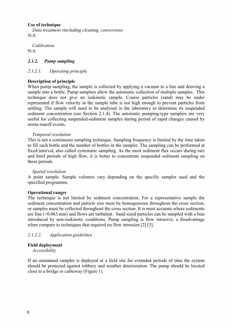
If an unmanned sampler is deployed at a field site for extended periods of time the system should be protected against robbery and weather deterioration. The pump should be located close to a bridge or cableway (Figure 1).

8

9

FIG. 1. Installation of a pumping station [4].

Pump samplers can be powered with batteries or they can be connected to a local mains power supply. Solar panels are often used to charge batteries at locations where it is not possible to use mains power.

Manpower Pump samplers are often automated, which eliminates the need for personnel to be present to take samples. However, installation of an automatic pumping sampler requires thorough planning. A field scientist should be available for collecting periodic reference samples.

Regulation N/A

Maintenance Regular visits should be made to check batteries and clean sampler hose intakes.


N/A

Calibration The major concern is the relation between the data and the true mean suspended-sediment concentration in transport at the time of the sample collection. Sediment samples collected from automatic sampling equipment must be calibrated to samples collected from cross-section depth-integrated or point-integrated samples for reliable results.

2.1.3. Isokinetic sampling


Description of principle The sampler is usually made of a plastic bottle with a water inlet nozzle and an air outlet. The diameter of the water inlet can be selected (or changed) so that the sampler will fill more or less quickly, depending on the depth of the river. Isokinetic sampling occurs when water velocity through the inlet nozzle is equal to the water velocity at the depth of the sampler.

9

10

Isokinetic samplers are divided into two categories; depth-integrating and point-integrating.

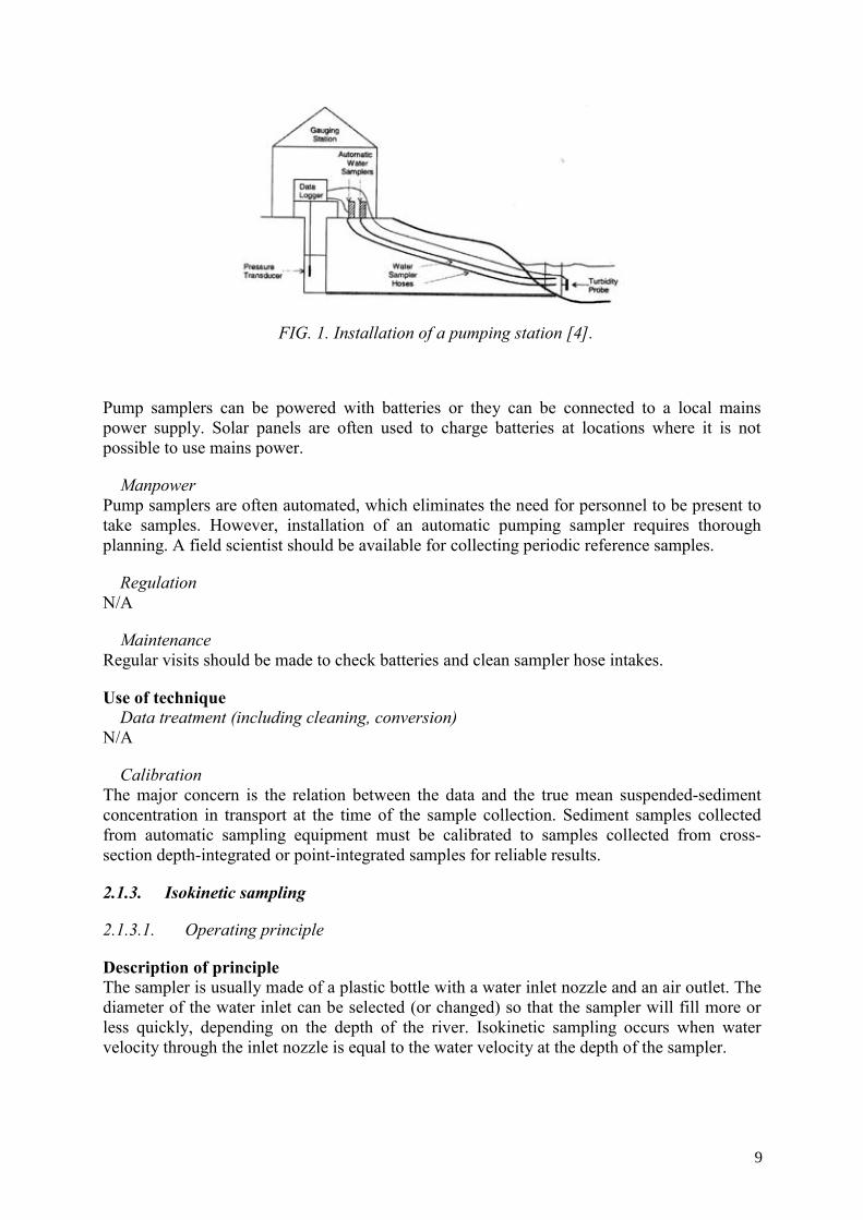
— Depth-integrating samplers (FIG.2) are lowered to the river bottom, then immediately raised to the surface; lowering and rising should be done at the same rate. The water-sediment sample collected will be proportional to the instantaneous stream velocity at the locus of the intake nozzle.

FIG. 2. Depth-integrated sampler model US-DH-59 (FISP).

— A point-integrating sampler uses an electrically activated valve to open and close the intake and exhaust passage.

The sample will need to be analysed in the laboratory to determine its suspended sediment concentration (see Section 2.1.4). The technique allows the determination of the suspended sediment concentration and particle size distribution.

Temporal resolution Temporal resolution is limited by available manpower. The technique is commonly used for weekly/monthly sampling.

Spatial resolution A depth-profile. The maximum distance the depth-integrating sampler can travel through the water column and still sample isokinetically is about 5 m at sea level. General field practice limits the use of the technique to depth of 4.6 m [5]. The point-integrating samplers are more versatile than the simpler depth-integrating types. They can be used to collect a suspended-sediment sample at any point from the surface of a stream to within approx. 10–15 cm of the bed, as well as to integrate over a range of depth.

Operational ranges The technique is not limited by sediment concentration. Isokinetic sampling is important for larger particles, such as sand, because the sampler would otherwise tend to over- or under-estimate the amount of suspended sediment. Errors caused by lack of isokinetic sampling are minimal for small particles (< 0.063 mm) and for practical purposes can be ignored.



The technique is applicable in any situation where the user has safe access to the water (e.g. from bridge, boat or wading). It can be used easily in remote places.

Power supply N/A

10

11

Manpower A boat is necessary if the river is large and the sampling is done in the middle of the river. Personnel must be on-hand to take samples.


Maintenance Thoroughly clean sample bottle and ensure sampler intake nozzle is clean.


N/A

Calibration N/A

2.1.4. Sample analysis

Suspended sediment concentration and particle size distribution may be determined through the laboratory analysis of grab, pump, or isokinetic samples. Other parameters such as contaminants could also be analysed but this aspect is beyond the scope of this report.

2.1.4.1. Suspended-sediment concentration

Evaporation and filtration are the two most frequently used methods for determining sediment concentration.

Filtration is faster and this is recommended when the quantity of sediment is small and/or coarse grained. Sample size, and filter paper pore size and diameter depend on the suspended sediment concentrations of the samples being analysed. Sample volumes of 500 ml are typically collected when analysing suspended sediment concentrations of UK Rivers (concentrations typically 10s to 100s of mg.l-1). Glass fibber filter disks of 47 mm or 90 mm diameter are often used.

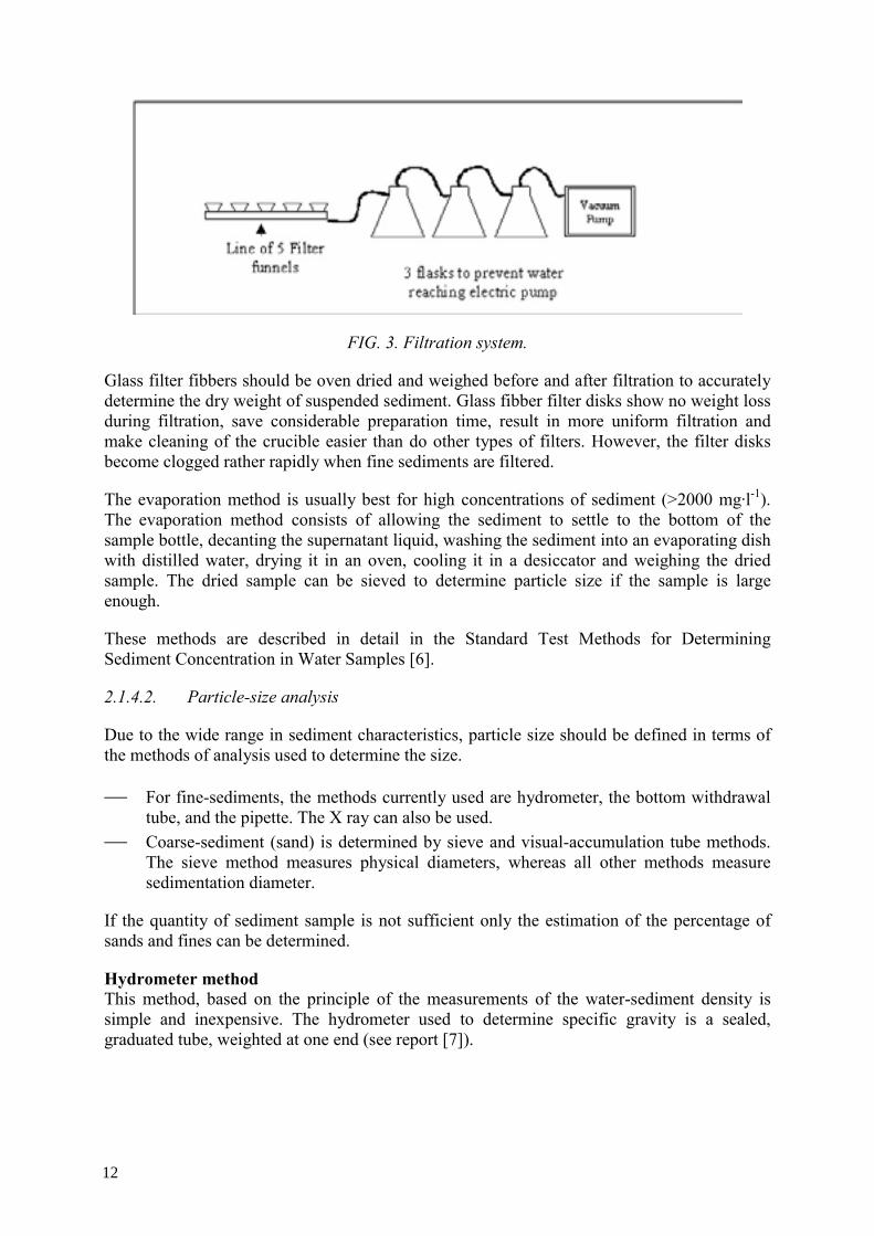
A typical filtration system, illustrated in Figure 3 would include the following:

(a) A three-piece filter funnel (borosilicate glass with acrylic plate 90 mm filter diameter 200ml reservoir volume);

(b) Oil free vacuum pump;

(c) Filter flask and overflow flasks;

(d) Multifilter holder is desirable to increase efficiency.

11

12

FIG. 3. Filtration system.

Glass filter fibbers should be oven dried and weighed before and after filtration to accurately determine the dry weight of suspended sediment. Glass fibber filter disks show no weight loss during filtration, save considerable preparation time, result in more uniform filtration and make cleaning of the crucible easier than do other types of filters. However, the filter disks become clogged rather rapidly when fine sediments are filtered.

The evaporation method is usually best for high concentrations of sediment (>2000 mg·l-1). The evaporation method consists of allowing the sediment to settle to the bottom of the sample bottle, decanting the supernatant liquid, washing the sediment into an evaporating dish with distilled water, drying it in an oven, cooling it in a desiccator and weighing the dried sample. The dried sample can be sieved to determine particle size if the sample is large enough.

These methods are described in detail in the Standard Test Methods for Determining Sediment Concentration in Water Samples [6].

2.1.4.2. Particle-size analysis

Due to the wide range in sediment characteristics, particle size should be defined in terms of the methods of analysis used to determine the size.

For fine-sediments, the methods currently used are hydrometer, the bottom withdrawal tube, and the pipette. The X ray can also be used.

Coarse-sediment (sand) is determined by sieve and visual-accumulation tube methods. The sieve method measures physical diameters, whereas all other methods measure sedimentation diameter.

If the quantity of sediment sample is not sufficient only the estimation of the percentage of sands and fines can be determined.

Hydrometer method This method, based on the principle of the measurements of the water-sediment density is simple and inexpensive. The hydrometer used to determine specific gravity is a sealed, graduated tube, weighted at one end (see report [7]).

12

13

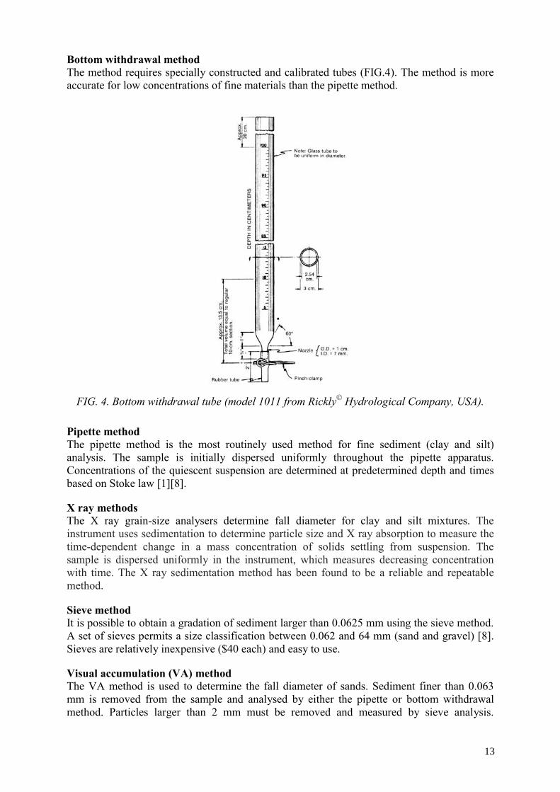
Bottom withdrawal method The method requires specially constructed and calibrated tubes (FIG.4). The method is more accurate for low concentrations of fine materials than the pipette method.

FIG. 4. Bottom withdrawal tube (model 1011 from Rickly© Hydrological Company, USA).

Pipette method The pipette method is the most routinely used method for fine sediment (clay and silt) analysis. The sample is initially dispersed uniformly throughout the pipette apparatus. Concentrations of the quiescent suspension are determined at predetermined depth and times based on Stoke law [1][8].

X ray methods The X ray grain-size analysers determine fall diameter for clay and silt mixtures. The instrument uses sedimentation to determine particle size and X ray absorption to measure the time-dependent change in a mass concentration of solids settling from suspension. The sample is dispersed uniformly in the instrument, which measures decreasing concentration with time. The X ray sedimentation method has been found to be a reliable and repeatable method.

Sieve method It is possible to obtain a gradation of sediment larger than 0.0625 mm using the sieve method. A set of sieves permits a size classification between 0.062 and 64 mm (sand and gravel) [8]. Sieves are relatively inexpensive ($40 each) and easy to use.

Visual accumulation (VA) method The VA method is used to determine the fall diameter of sands. Sediment finer than 0.063 mm is removed from the sample and analysed by either the pipette or bottom withdrawal method. Particles larger than 2 mm must be removed and measured by sieve analysis.

13

Sediment is added at the top of a settling tube and the deposited sediment is stratified according to the settling velocities of the various particles in the mixture. The tube must be certified [1].

2.2. Optical

2.2.1. Scattering


Description of principle During optical backscatter sensing, infrared or visible light is directed into the sample volume. A portion of the light will be backscattered if particles are in suspension. A series of photodiodes positioned around the emitter detect the backscattered signal. The strength of this backscattered signal is used to determine the turbidity of the solution. Optical backscatter sensors are available as small cylinders with an optical window at one end, a cable connection at the other end, and an encased circuit board.

Temporal resolution Good temporal resolution. Readings may be made at very high temporal resolution (e.g. a reading a second). The temporal resolution is limited by the capacity of the data logger memory relative to the downloading frequency. Turbidity is measured in real time. Therefore, a quasi-continuous record of turbidity is possible.

Spatial resolution An optical backscatter sensor makes a point measurement (volume contained within a few centimeters of the end of the probe). The size of the point varies with the turbidity. The sample volume will be smaller when the turbidity is higher and larger when the turbidity is lower.

Operational ranges Optical backscattering (nephelometric) turbidity sensors are more widely used than those based on the transmission principle. They are commonly used to accurately measure turbidities ranging from 0 to at 3,000 NTU. A turbidity of 3000 NTU typically corresponds to a suspended sediment concentration of 3 g/l but this will vary depending on the characteristics of the particles in suspension. Probes specifically designed for measuring higher turbidities (up to 30,000 NTU) are also available. Optical backscattering probes are available from several manufacturers (e.g. see www.planet-ocean.co.uk). Analite nephelometric turbidity probes are commonly used. They are relatively insensitive to temperature changes (coefficient of <+/- 0.05%.˚C-1 for temperature range 0 to 40˚C) and use infrared light sources so there is very little interference from ambient light.

Optical sensors are most suited to measuring the turbidity of suspensions of fine sediment with a uniform particle size. Sensitivity to the fines is much greater than to fine sands. Turbidity measurements are affected by particle shape, composition, and water color [9].

Sediment particle size has a major effect on the turbidity measurement. For a given sediment concentration a reduction in particle size results in an increase in turbidity [10]. OBS performs well for measuring concentrations where particle size is constant or remains in 0.2–0.4 mm range [11]. They work well in UK rivers where >90% of particles are <0.063 mm.

14

15



User needs access to water to clean sensors. Alternatively, sensors could be lifted from the water for cleaning. The instrument should ideally be mounted in a protective cage in fast flowing water that has a suspended sediment concentration that is representative of the cross section. Areas of turbulent water should be avoided as air bubbles can affect the readings. For some instruments remote-deployment is possible.

Power supply The devices require little power. They are often powered by batteries. The batteries may be charged by solar panel or mains electricity.

Manpower Manpower for cleaning sensors and downloading data is an essential requirement. Basic training in using data loggers is essential. Loggers could be downloaded by using telemetry but site visits would still be necessary to clean sensors. Laboratory analysis will be necessary to calibrate turbidity sensors. However, data are automatically recorded between site visits so manpower can be drastically reduced.

Regulation Permission for installation will be required from landowner.

Maintenance Sensor lenses should be cleaned frequently. Sensors are now available with lens wipers. This helps keep lenses clean but weekly/fortnightly cleaning is still recommended. In warm nutrient rich waters bio-fouling may occur rapidly and the probes may need cleaning more often. In cold turbid environments (e.g. glacial rivers) weekly cleaning may not be necessary.


Output from turbidity meters is in mV and data loggers usually store this data every x minutes. Recorded data should be regularly downloaded from the data logger onto a computer or storage module. The voltage output from the sensor should be converted to standard Nephelometric Turbidity Units (NTU). It is recommended that calibrations are undertaken using certified polymer bead solutions. AMCO polymer bead solutions are approved by the USEPA (see www.apsstd.com). It is not recommended that Formazin be used, as it is a suspected carcinogen. Calibration to standard units allows sensor drift to be identified and compensated. Sensors may drift significantly due to aging electronic components and lens scratching. Calibrations should be undertaken on a three monthly basis. The standard turbidity data are then quality controlled to remove erroneous data. These data usually result from debris becoming trapped on the sensor head or algal growth on the sensor lens. They may be identified as very high constant values, highly variable values, or steadily increasing values not related to changes in river stage. If there is evidence of linear drift in the output between cleaning intervals a linear correction may be used.

It is also recommended to use the optical sensor along with another type of sensor such as acoustic backscatter or in situ particle sizing sensor.

15

16

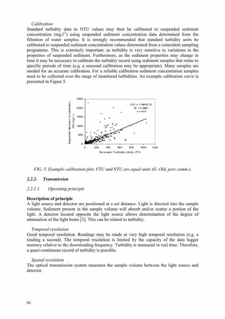
Calibration Standard turbidity data in NTU values may then be calibrated to suspended sediment concentration (mg.l-1) using suspended sediment concentration data determined from the filtration of water samples. It is strongly recommended that standard turbidity units be calibrated to suspended sediment concentration values determined from a coincident sampling programme. This is extremely important, as turbidity is very sensitive to variations in the properties of suspended sediment. Furthermore, as the sediment properties may change in time it may be necessary to calibrate the turbidity record using sediment samples that relate to specific periods of time (e.g. a seasonal calibration may be appropriate). Many samples are needed for an accurate calibration. For a reliable calibration sediment concentration samples need to be collected over the range of monitored turbidities. An example calibration curve is presented in Figure 5.

FIG. 5. Example calibration plot. FTU and NTU are equal units (G. Old, pers comm.).

2.2.2. Transmission


Description of principle A light source and detector are positioned at a set distance. Light is directed into the sample volume. Sediment present in the sample volume will absorb and/or scatter a portion of the light. A detector located opposite the light source allows determination of the degree of attenuation of the light beam [3]. This can be related to turbidity.

Temporal resolution Good temporal resolution. Readings may be made at very high temporal resolution (e.g. a reading a second). The temporal resolution is limited by the capacity of the data logger memory relative to the downloading frequency. Turbidity is measured in real time. Therefore, a quasi-continuous record of turbidity is possible.

Spatial resolution The optical transmission system measures the sample volume between the light source and detector.

16

17

Operational ranges Sensors based on the transmission principle (absorptiometric) are often used for monitoring lower turbidities and suspended sediment concentrations (often <1g l-1) than sensors operating with the scattering principle (see above). Nevertheless, absorptiometric sensors may be used to monitor suspended sediment concentrations from 0 to at least 20 g/l (e.g. Partech IR8). However, if measuring high concentrations the measurement gap on the sensor becomes very small and prone to becoming clogged with debris. For example, the measurement gap on the Partech IR8 sensor is just 8mm. Absorptiometric sensors rely on keeping two lenses clean (receiver and detector) and are sensitive to the nature of suspended particles (e.g. their refractive index).

Absorptiometric turbidity sensors are available from Partech (see http://www.keison.co.uk/ partech/partech5.htm). Partech probes use infrared light sources so there is little interference from ambient light.



See Section 2.2.1.2.

Power supply See Section 2.2.1.2.

Manpower See Section 2.2.1.2.

Regulation See Section 2.2.1.2.

Maintenance See Section 2.2.1.2. Clean weekly using a soft toothbrush.

The sensors are small and should be cleaned from time to time in order to avoid measurements errors due to algal growth, tannin accumulation, fouling. They can be used for a wide variety of monitoring tasks in industrial, laboratory, riverine, estuarine, and oceanic settings.

Use of technique See Section 2.2.1.2.

2.3. Nuclear

2.3.1. Scattering


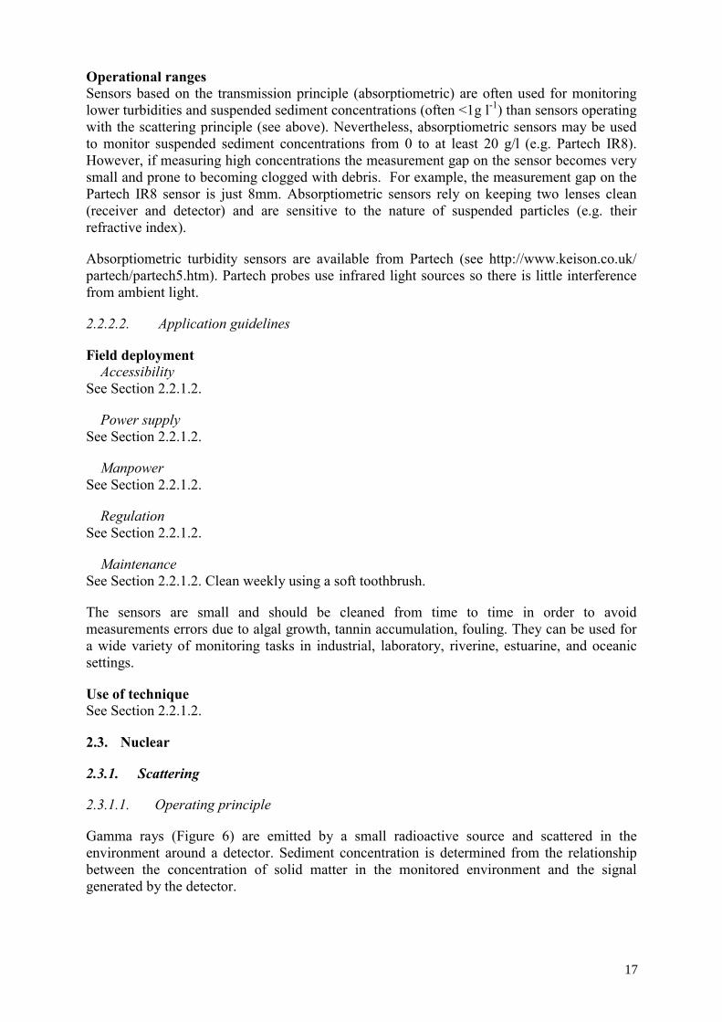
Gamma rays (Figure 6) are emitted by a small radioactive source and scattered in the environment around a detector. Sediment concentration is determined from the relationship between the concentration of solid matter in the monitored environment and the signal generated by the detector.

17

18

FIG. 6. Operating principle of the nuclear scattering system.

The number of photons N measured by the detector is a function of sediment concentration and is related to the number No of photons measured in pure water by the equation:

N/No = (k . ρm )n . exp ( - k . ρm) (1)

Where: k and n are constants characteristics of the gauge ρm is the density of the mixture water + sediment

The sources normally used for scattering gauges are 137Cs (mainly) and 241Am.

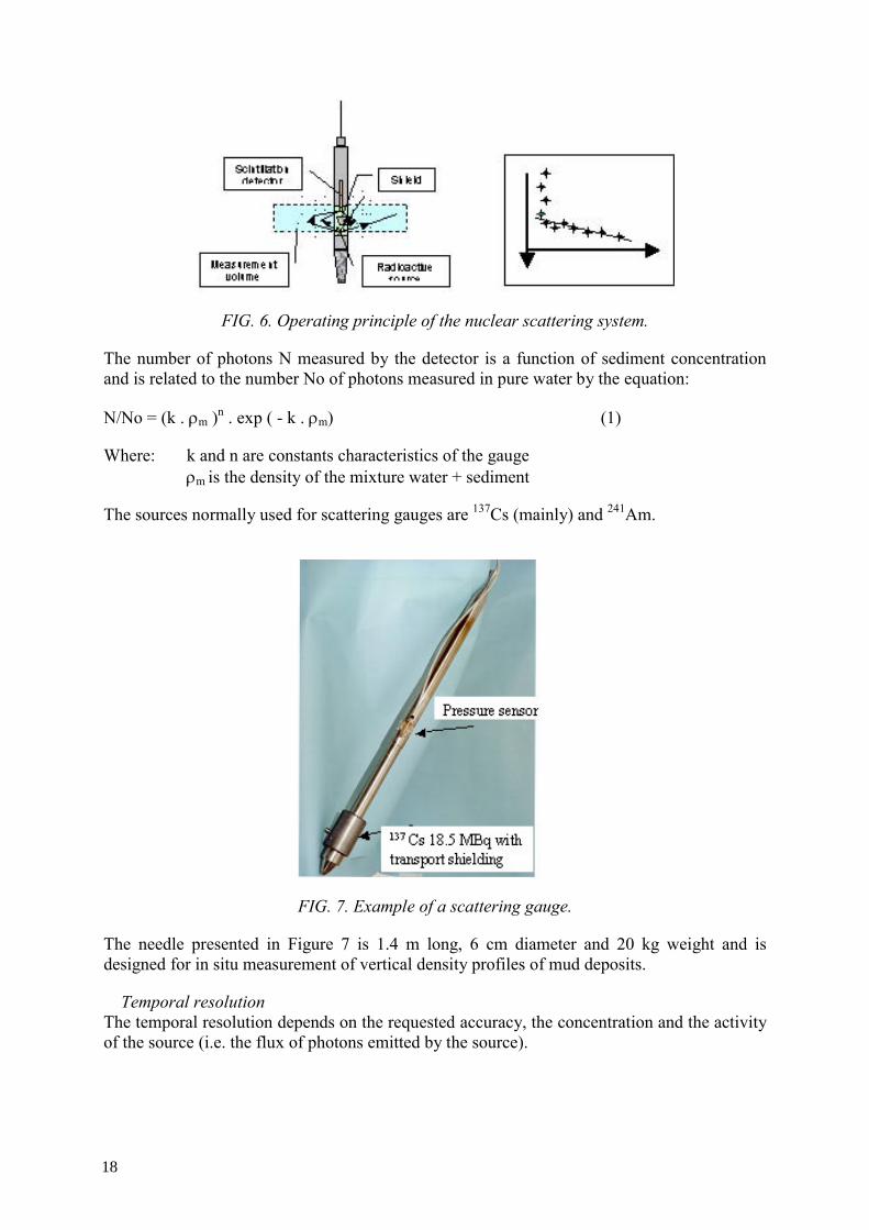
FIG. 7. Example of a scattering gauge.

The needle presented in Figure 7 is 1.4 m long, 6 cm diameter and 20 kg weight and is designed for in situ measurement of vertical density profiles of mud deposits.

Temporal resolution The temporal resolution depends on the requested accuracy, the concentration and the activity of the source (i.e. the flux of photons emitted by the source).

18

19

For example, the measurement time will be 10 seconds for a 137Cs source (18.5 MBq), a concentration of 300 g.l-1 and an accuracy of ± 10 g.l-1 (68% confidence level). Practically the measurement time can vary between 1 sec and 1000 sec (or more).

Spatial resolution The measurement volume is usually big. In the case of the gauge shown in Figure 7, it is 10 cm thickness and 70 cm diameter.

Operational ranges This type of instrument has a measurement range which encompasses sediment concentration between 20 and 1000 g.l-1.

All the parameters described above (temporal resolution, spatial resolution and measurement range) can be redefined for any measurement problem. However, the device is mainly used for high concentration measurement.



The technique is applicable in any situation where the user has safe access to the water (e.g. from bridge, boat or wading). It can be used easily in remote places.

The scattering gauges are used mainly for bed density measurements (harbour basins, dam reservoir, lagoon, muddy areas...). They are generally deployed from a small boat. The probe is lowered using a suspension cable to sink into the soft bed under its own weight. In this case, probe depth is given by a pressure sensor. Vertical profiles of concentration (i.e. density) are recorded along a grid in order to map the measurement area.

Power supply The power supply is depending on the accessories of the system:

For static or manually operated probe connected to a data logger, the power supply is generally a simple 12V DC battery included in the data logger and allows autonomous data collection for several days. An external battery or a solar panel can also be added to increase the deployment time.

With a probe connected to a computer through a 12 or 24 V DC winch, it is necessary to use an external battery (car type).

In particular cases it is necessary to use a 220 V AC winch that requires a power generator.

Manpower We can consider two operational cases:

Utilization at fixed point to measure suspended sediment concentration in a stream: The installation of the device can be realized by one or two workers with some training regarding the use of the system and regulation and safety procedures.

Utilization from a boat to measure vertical profiles of concentration in mud deposits: at least two persons are necessary, one for the gauge, and one for the boat.

19

20

In both case it is necessary to have one person trained on safety procedures and having some knowledge on radioactivity regulation.

Regulation The use of ionizing radiation requires a clearance to be obtained from the radiological safety board and the nuclear safety authority of the country. To obtain this clearance it is necessary to present a document with the characteristics of the gauge (nature and activity of the source, map of the dose rate around the system) and the scheduled use of the system. The radiological characteristics of the gauge are part of the documents given by the gauge supplier. One person of the company using the gauge will have to be trained (officially) to know the country regulation on ionizing radiation management in order to be able to manage the gauge and its use.

Maintenance There are two main aspects:

Electronic maintenance: the electronic cards used in such probes are generally quite simple and rugged, and require little maintenance. It is generally useful to check the settings of the card and the threshold adjustment one or twice a year using an oscilloscope.

General maintenance: when the system is installed at a fixed point for a long time it is necessary to clean the instrument and its surroundings on a weekly basis.


The raw data are classically saved in text or spreadsheet files.

The first step of the treatment is to convert data into a user defined unit (g.l-1 or density). A simple algorithm can be applied using the equation (1) including the coefficients determined by the calibration. It can be included in the data acquisition software or written by the operator under Microsoft Excel or any type of programming language. It is also possible at this stage to clean the data by smoothing, aggregation, or erasing the wrong data if any, etc.

The second step concerns the exploitation of the physical parameter itself. This step depends on the objectives of the experiment and on the site.

Suspended sediment concentration is interesting by itself but the interest will be more important if it is possible to also measure at the same time the water flow rate. The integration of the information will give the mass transported by the flow and the relationship between flow rate and concentration.

The exploitation of vertical profiles of mud deposited in harbour basins, dam reservoirs… will take a greater value if they are shown as a map. This treatment can easily be done using a Geographical Information System. Obviously this type of mapping will require on site a Global Positioning System.

Calibration The correct functioning of a nuclear gauge depends on calibration undertaken both in the laboratory and in situ. Calibration is carried out in tanks using sediment samples from the site selected for concentration measurement.

20

21

A calibration curve is obtained by relating the counting rate N to the varying suspended sediment concentration values.

The relative sensitivity of measurement is the ratio of the relative change in counting rate to the relative change in sediment concentration. The sensitivity is greater at lower energies because of the increased difference between ρs and ρw. Very low energy problems arise from the increased influence of variations in chemical composition of sediments.

2.3.2. Transmission


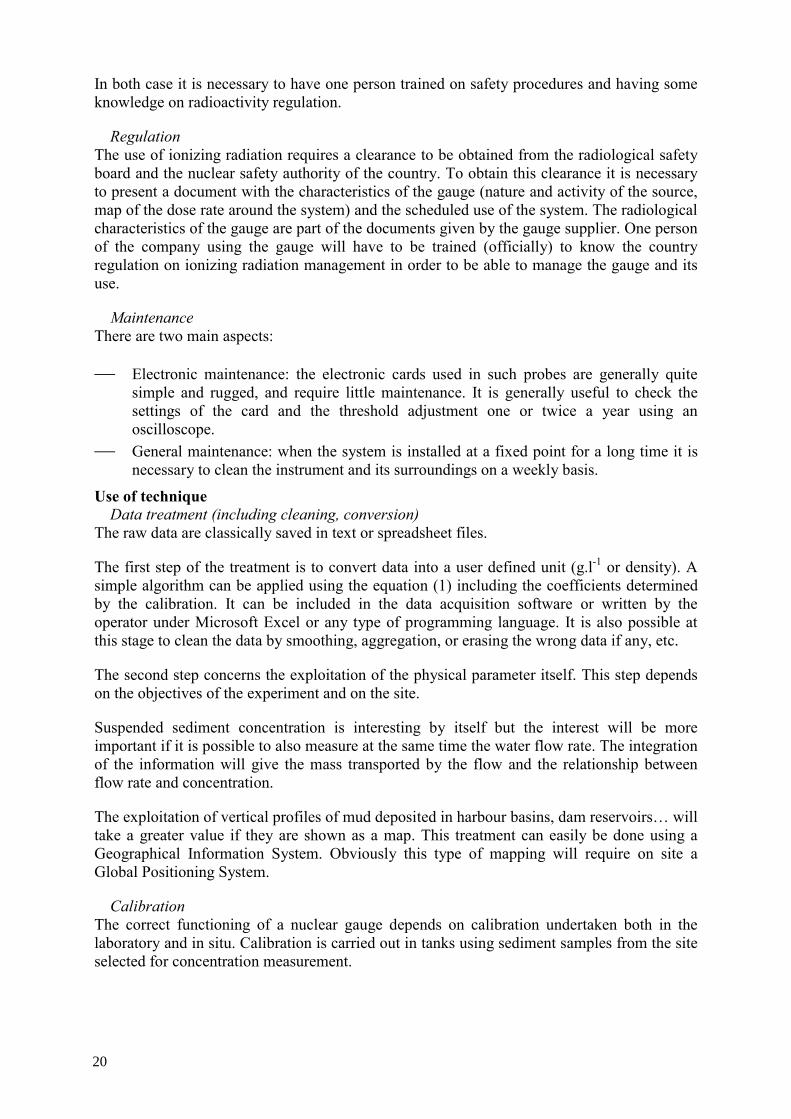
Description of principle The measurement is based on the attenuation, by the sediments of gamma rays from a radioactive sealed source emitted in the direction of the detector (Figure 8).

FIG. 8. Schema of the nuclear transmission measurements principles.

The number N of monoenergetic (or not) photons transmitted through x cm of water containing a concentration C by weight of sediment is related to the number No of photons transmitted through the same thickness of pure water by the equation:

N/No = exp(- (µ s.ρs-µw.ρw).C.ρm.x / ρs ) (2)

The sensitivity (i.e. contrast) and thus accuracy of the measurements increase when the radiation energy decreases. The measurement depends on the chemical composition of the measured sediment. A compromise has to be defined between the sensitivity of the concentration measurement and the sensitivity of the instrument to the variations of the sediment composition.

21

22

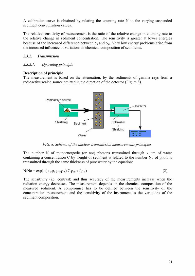
FIG. 9. Influence of the gamma ray energy on the contrast for a transmission gauge designed with a classical geometry (distance source-detector 20cm, low collimation).

Practically speaking, the instruments are more efficient if they are designed or adapted to each particular situation and have to be calibrated with the sediments, which will have to be measured on the site.

From these considerations it is possible to give some typical values of the measurement precision for some classical gauges (Table 2).

Table 2. Typical values of the measurement precision for some classical gauges

Energy (keV)

Thickness of the measurement cell (cm)

Counting rate (c·s-1)

Counting time (s)

Measurement uncertainty at 65% confidence

30 5 40000 300 0.09 g/l

60 17 11000 300 0.28 g/l

662 30 30000 300 0.5 g/l

The transmission gauge can be static (installed in a stream at a fixed point, Figure 10) or mobile (submerged or measuring in a pumping circuit, Figure 11).

22

23

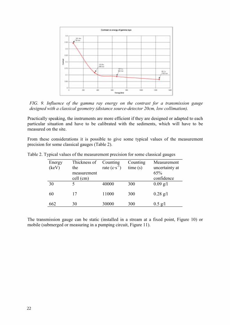
FIG. 10. Scheme of a static gauge installed at a fixed point in a stream.

With the system shown in Figure 10, it is possible to acquire the data from three gauges simultaneously, installed for example at three different depths in the channel.

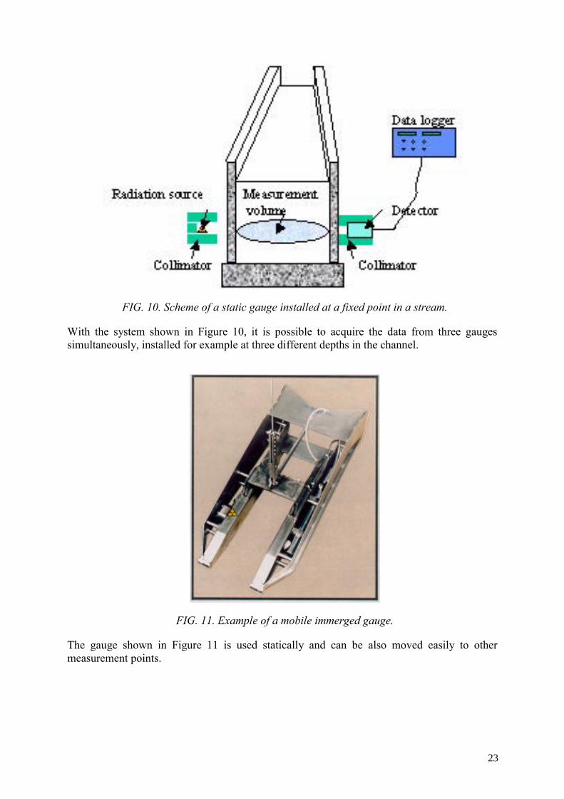
FIG. 11. Example of a mobile immerged gauge.

The gauge shown in Figure 11 is used statically and can be also moved easily to other measurement points.

23

24

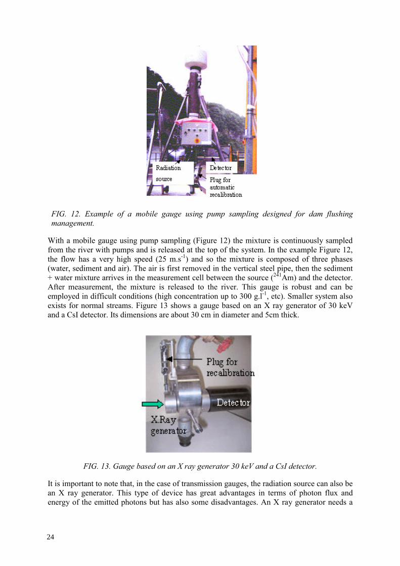
FIG. 12. Example of a mobile gauge using pump sampling designed for dam flushing management.

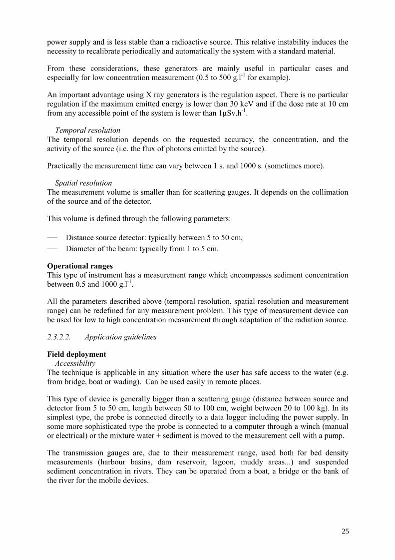
With a mobile gauge using pump sampling (Figure 12) the mixture is continuously sampled from the river with pumps and is released at the top of the system. In the example Figure 12, the flow has a very high speed (25 m.s-1) and so the mixture is composed of three phases (water, sediment and air). The air is first removed in the vertical steel pipe, then the sediment + water mixture arrives in the measurement cell between the source (241Am) and the detector. After measurement, the mixture is released to the river. This gauge is robust and can be employed in difficult conditions (high concentration up to 300 g.l-1, etc). Smaller system also exists for normal streams. Figure 13 shows a gauge based on an X ray generator of 30 keV and a CsI detector. Its dimensions are about 30 cm in diameter and 5cm thick.

FIG. 13. Gauge based on an X ray generator 30 keV and a CsI detector.

It is important to note that, in the case of transmission gauges, the radiation source can also be an X ray generator. This type of device has great advantages in terms of photon flux and energy of the emitted photons but has also some disadvantages. An X ray generator needs a

24

25

power supply and is less stable than a radioactive source. This relative instability induces the necessity to recalibrate periodically and automatically the system with a standard material.

From these considerations, these generators are mainly useful in particular cases and especially for low concentration measurement (0.5 to 500 g.l-1 for example).

An important advantage using X ray generators is the regulation aspect. There is no particular regulation if the maximum emitted energy is lower than 30 keV and if the dose rate at 10 cm from any accessible point of the system is lower than 1µSv.h-1.

Temporal resolution The temporal resolution depends on the requested accuracy, the concentration, and the activity of the source (i.e. the flux of photons emitted by the source).

Practically the measurement time can vary between 1 s. and 1000 s. (sometimes more).

Spatial resolution The measurement volume is smaller than for scattering gauges. It depends on the collimation of the source and of the detector.

This volume is defined through the following parameters:

Distance source detector: typically between 5 to 50 cm, Diameter of the beam: typically from 1 to 5 cm.

Operational ranges This type of instrument has a measurement range which encompasses sediment concentration between 0.5 and 1000 g.l-1.

All the parameters described above (temporal resolution, spatial resolution and measurement range) can be redefined for any measurement problem. This type of measurement device can be used for low to high concentration measurement through adaptation of the radiation source.



The technique is applicable in any situation where the user has safe access to the water (e.g. from bridge, boat or wading). Can be used easily in remote places.

This type of device is generally bigger than a scattering gauge (distance between source and detector from 5 to 50 cm, length between 50 to 100 cm, weight between 20 to 100 kg). In its simplest type, the probe is connected directly to a data logger including the power supply. In some more sophisticated type the probe is connected to a computer through a winch (manual or electrical) or the mixture water + sediment is moved to the measurement cell with a pump.

The transmission gauges are, due to their measurement range, used both for bed density measurements (harbour basins, dam reservoir, lagoon, muddy areas...) and suspended sediment concentration in rivers. They can be operated from a boat, a bridge or the bank of the river for the mobile devices.

25

26

For bed density measurement, a small boat (rubber boat for ex.) is generally required. The probe is lowered on a suspension cable to sink into the soft bed under its own weight. In this case the probe depth is given by a pressure sensor. Vertical profiles of concentration (i.e. density) are recorded along a grid in order to map the measurement area.

For suspended sediment concentration measurement, the probe is towed by a cable at a defined depth in the stream or can be moved in the cross section (vertically and horizontally) to obtain the concentration field.

In these two cases, the weight can be an advantage for the penetration of the probe in mud deposits and for having a good stability in the stream. The probe shown in Figure 11 (weight 120 kg) is currently used in streams with a velocity greater than 3 m.s-1.

For static measurement the device has to be installed in a concrete channel. The main problem for the static systems is, as for the optical systems, to be sure of its representativity and also to be sure of the stability of the river bed.

Power supply The power supply is depending on the accessories used.

In the simplest case (static or manually operated probe connected to a data logger), the power supply is generally a simple 12V DC battery included in the data logger allowing autonomy of some days. An external battery or a solar panel can also be added to increase the autonomy.

In a more sophisticated case (probe connected to a computer through a 12 or 24V DC winch), it will be necessary to use an external battery (car type).

In particular cases it is necessary to use a 220V AC winch or a pump and so to use a power generator or to have a connection to the mains.

Manpower We can consider two operational cases:

Utilization at fixed point to measure suspended sediment concentration in a stream: the installation of the device can be realized by one or two workers with some training regarding the use of the system and regulation and safety procedures.

Utilization from a boat to measure vertical profiles of concentration in mud deposits: at least two persons are necessary, one for the gauge, and one for the boat.

In both case it is necessary to have one person trained on safety procedures and having some knowledge on radioactivity regulation.

Regulation The use of ionizing radiation requires a clearance to be obtained from the radiological safety board and the nuclear safety authority of the country. To obtain this clearance it is necessary to present a document containing the characteristics of the gauge (nature and activity of the source, map of the dose rate around the system) and the scheduled use of the system. The radiological characteristics of the gauge are a part of the file given by the gauge supplier. One person of the company using the gauge will have to be trained (officially) to know the country regulation on ionizing radiation management and so, to be able to manage the gauge and its use.

26

27

Maintenance There are two main aspects:

Electronic maintenance: the electronic cards used in such probes are generally quite simple and rugged, and require little maintenance. It is generally useful to check the settings of the card and the threshold adjustment one or twice a year using an oscilloscope.

General maintenance: when the system is installed at a fixed point for a long time it is necessary to clean the instrument and its surroundings on a weekly basis.


The process is described in section 2.3.1.3.

The first step in data treatment is to convert raw data into a user defined unit (g.l-1 or density). A simple algorithm can be applied using the equation (1) including the coefficients determined by the calibration. It can be included in the data acquisition software or written by the operator under Microsoft Excel or any type of programming language. It is also possible at this stage to clean the data by smoothing, aggregation, erasing the wrong data if any, etc.

The second step concerns the exploitation of the physical parameter itself. This step depends on the problem and on the site.

Suspended sediment concentration is interesting by itself but the interest will be more important if it is possible to measure at the same time the water flow rate. The integration of the information will give the mass transported by the flow and the relationship between flow rate and concentration. The exploitation of vertical profiles of mud deposited in harbour basins, dam reservoirs, etc. will take a greater value if they are shown as a map. This treatment can easily be done using Geographic Information System. Obviously this type of mapping will require on site a Global Positioning System.

Calibration A calibration curve is obtained by relating the counting rate N to the varying suspended sediment concentration values.

The relative sensitivity of measurement is the ratio of the relative change in counting rate to the relative change in sediment concentration. The sensitivity is greater at lower energies because of the increased difference between ρs and ρw. Very low energy problems arise from the increased influence of variations in chemical composition of sediments.

2.4. Acoustic (single frequency)

2.4.1. Operating principle

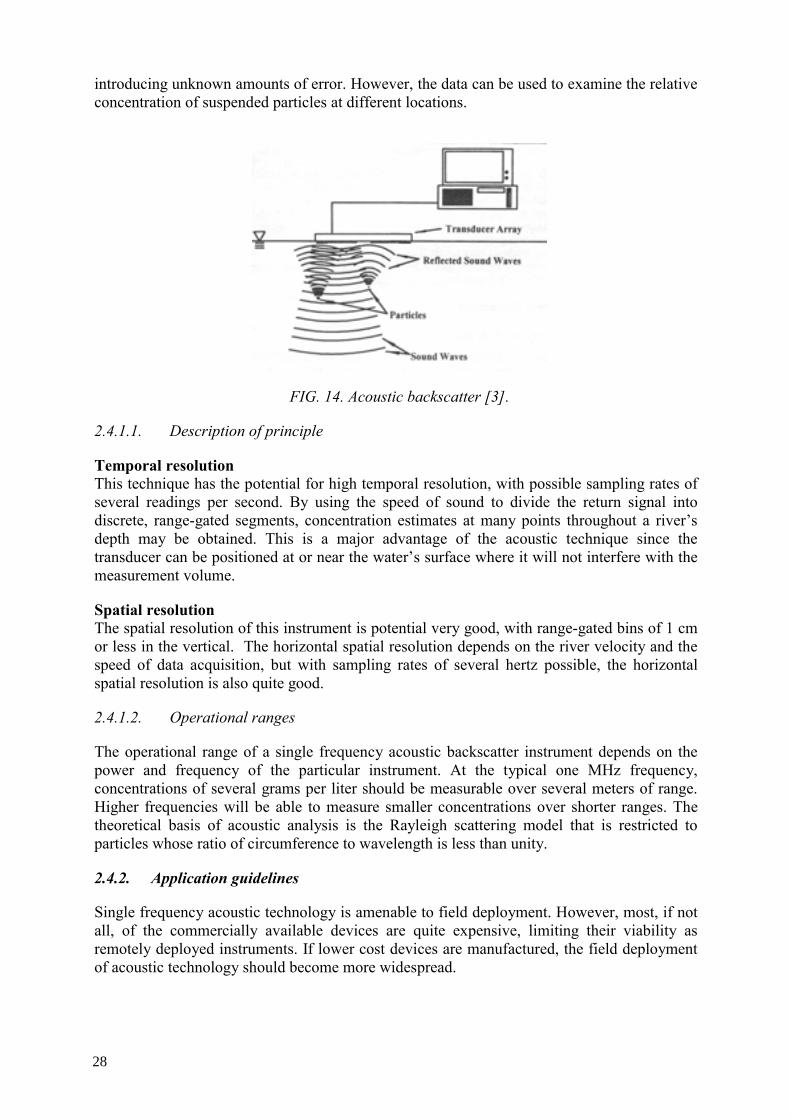
High frequency sound, usually in the megahertz range, is propagated through the water/sediment mixture from an acoustic transducer that can be used to transmit and receive signals. When the sound waves impact suspended particles, a portion of the sound is scattered back toward the transducer where it produces an electrical signal. The amplitude of this backscattered sound is recorded. If particle size information is available, the backscatter data can be used to estimate suspended-sediment concentration over the range through which the signal was propagated. If no particle size information is available, the size of the suspended material must be estimated based on measurements of the size distribution of the bed material,

27

28

introducing unknown amounts of error. However, the data can be used to examine the relative concentration of suspended particles at different locations.

FIG. 14. Acoustic backscatter [3].

2.4.1.1. Description of principle

Temporal resolution This technique has the potential for high temporal resolution, with possible sampling rates of several readings per second. By using the speed of sound to divide the return signal into discrete, range-gated segments, concentration estimates at many points throughout a river’s depth may be obtained. This is a major advantage of the acoustic technique since the transducer can be positioned at or near the water’s surface where it will not interfere with the measurement volume.

Spatial resolution The spatial resolution of this instrument is potential very good, with range-gated bins of 1 cm or less in the vertical. The horizontal spatial resolution depends on the river velocity and the speed of data acquisition, but with sampling rates of several hertz possible, the horizontal spatial resolution is also quite good.

2.4.1.2. Operational ranges

The operational range of a single frequency acoustic backscatter instrument depends on the power and frequency of the particular instrument. At the typical one MHz frequency, concentrations of several grams per liter should be measurable over several meters of range. Higher frequencies will be able to measure smaller concentrations over shorter ranges. The theoretical basis of acoustic analysis is the Rayleigh scattering model that is restricted to particles whose ratio of circumference to wavelength is less than unity.

2.4.2. Application guidelines

Single frequency acoustic technology is amenable to field deployment. However, most, if not all, of the commercially available devices are quite expensive, limiting their viability as remotely deployed instruments. If lower cost devices are manufactured, the field deployment of acoustic technology should become more widespread.

28

29

2.4.2.1. Field deployment

Accessibility There are no specific accessibility issues for using acoustic technology. The acoustic transducer must be in contact with or below the water surface so that the acoustic signal can be transmitted and received. A suitable location should also include a place to mount a pump sampler so that calibration samples can be collected. The pump sampler nozzle should be located as near as possible to the sample volume of the acoustic device without interfering with acoustic measurements.

Power supply Acoustic technology has a relatively low power requirement since the duty cycle of the transmitter is usually well below 1%. More energy will be used by the analog to digital converter and data logging equipment. A solar cell and batteries should be able to support field deployment.

Manpower There are no special manpower requirements for the use of acoustic technology. Regular maintenance and data retrieval will be necessary, as well as collecting and analysing pump sample data. Biofouling does not usually present a problem since acoustic signals will propagate through it, but trash collected by the transducer will interfere with the signal.

Regulation N/A

Maintenance Maintaining a field deployment of an acoustic backscatter sensor will mainly involve insuring that there is no buildup of debris around and under the acoustic transducer.

2.4.2.2. Use of technique

Data treatment (including cleaning, conversion) For detailed discussions on single frequency acoustic data treatment, see [12]. There have been several approaches to the conversion of acoustic backscatter data into suspended-sediment concentration data. Signal loss due to spherical spreading, attenuation, absorption, and scattering must be accounted for. Errors in particle size estimation can result in significant concentration errors. In the absence of pump sample size distribution data, the particle size must be estimated based on measurements of the bottom sediment size distribution. However, it is likely that smaller size-fractions are suspended higher in the flow than larger ones, introducing an error of unknown amount. Using the size of the bottom sediments will yield more accurate results near the bed, where there are proportionately higher suspended particle concentrations.

Off-the-shelf equipment, such as Acoustic Doppler Current Profilers (ADCP), can be purchased to collect backscatter data. However, software for converting the backscattered signal amplitude into suspended particle concentration is not readily available.

Calibration The following section outlines an approach based on [17]. The following equation can be

used: xMBfVbin ρ∞= (3)

29

30

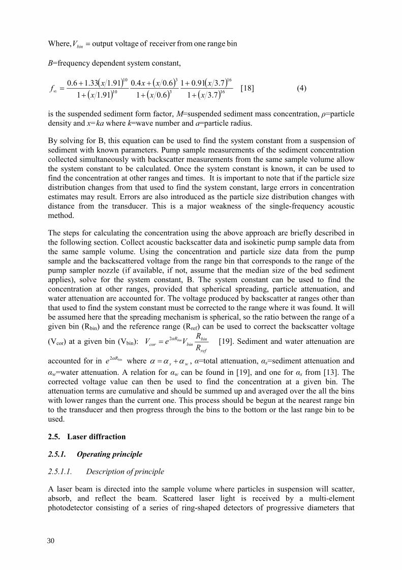
Where, bin range one fromreceiver of tageoutput vol=binV

B=frequency dependent system constant,

( )( )

( )( )

( )( )16

16

3

3

10

10

7.317.391.01

6.016.04.0

91.1191.133.16.0

xx

xxx

xxf

++

++

++

=∞ [18] (4)

is the suspended sediment form factor, M=suspended sediment mass concentration, ρ=particle density and x=ka where k=wave number and a=particle radius.

By solving for B, this equation can be used to find the system constant from a suspension of sediment with known parameters. Pump sample measurements of the sediment concentration collected simultaneously with backscatter measurements from the same sample volume allow the system constant to be calculated. Once the system constant is known, it can be used to find the concentration at other ranges and times. It is important to note that if the particle size distribution changes from that used to find the system constant, large errors in concentration estimates may result. Errors are also introduced as the particle size distribution changes with distance from the transducer. This is a major weakness of the single-frequency acoustic method.

The steps for calculating the concentration using the above approach are briefly described in the following section. Collect acoustic backscatter data and isokinetic pump sample data from the same sample volume. Using the concentration and particle size data from the pump sample and the backscattered voltage from the range bin that corresponds to the range of the pump sampler nozzle (if available, if not, assume that the median size of the bed sediment applies), solve for the system constant, B. The system constant can be used to find the concentration at other ranges, provided that spherical spreading, particle attenuation, and water attenuation are accounted for. The voltage produced by backscatter at ranges other than that used to find the system constant must be corrected to the range where it was found. It will be assumed here that the spreading mechanism is spherical, so the ratio between the range of a given bin (Rbin) and the reference range (Rref) can be used to correct the backscatter voltage

(Vcor) at a given bin (Vbin): ref

binbin

Rcor R

RVeV binα2= [19]. Sediment and water attenuation are

accounted for in binRe α2 where ws ααα += , α=total attenuation, αs=sediment attenuation and αw=water attenuation. A relation for αw can be found in [19], and one for αs from [13]. The corrected voltage value can then be used to find the concentration at a given bin. The attenuation terms are cumulative and should be summed up and averaged over the all the bins with lower ranges than the current one. This process should be begun at the nearest range bin to the transducer and then progress through the bins to the bottom or the last range bin to be used.

2.5. Laser diffraction



A laser beam is directed into the sample volume where particles in suspension will scatter, absorb, and reflect the beam. Scattered laser light is received by a multi-element photodetector consisting of a series of ring-shaped detectors of progressive diameters that

30

allow measurement of the scattering angle of the beam. Particle size can be calculated from knowledge of this angle, using the Fraunhofer approximation or the exact Lorenz-Mie solution. The main advantage of these instruments is that they permit the measurement of the size distribution and concentration of sediment in suspension.

Temporal resolution The sensors allow in situ continuous measurement.

Spatial resolution Point measurement only.


The laser-diffraction based sensors are designed to detect suspended particles over a size range of 0.0013–0.25 mm [20] By measuring the small-angle scattering; some instruments (LISST1 series for example) hold calibrations for wide range of sizes (200:1), regardless of particle composition. The instrument is not affected by the refractive index of the particles [21]. The simple sensors do not provide the possibility for separating measurements of sand from finer particles.



Accessibility The technique is applicable in any situation where the user has safe access to the water (e.g. from bridge, boat or wading). Can be used easily in remote places.

Power supply The laser sensors are using single voltage batteries. External AC power supply is also possible.

Manpower The laser sensors are usually installed at a fixed-depth near shore-side or river bank. Manpower is necessary for cleaning the instrument from time to time.

Regulation N/A

Maintenance Cleaning of the sensor and download of data when memory is full.


Data treatment (including cleaning, conversion) Scattering at 32 angles is the primary information that is recorded. This primary measurement is mathematically inverted to get the size distribution. The size distribution is presented as concentration (µl.l-1) in each of 32 log-spaced size bins. Optical transmission, water depth and temperature are recorded as supporting measurements. Data downloaded and displayed on a computer screen shows the volume concentration of particles, the Sauter Mean diameter 1 LISST: Laser In situ Scattering and Transmissometry, laser-based instrument manufactured by SEQUOIA, USA.

31

(SMD), and optical transmission. The calibration of the instrument remains constant as long as the size of particles is within a specified 200:1 range.

Calibration The instruments usually measure only the volumetric concentration and grain size of suspended particles. The user can estimate mass concentration once a suitable density conversion is gravimetrically determined [20].

2.6. Tracer techniques



The term ‘’tracer’’ is taken in sedimentology to mean any property or characteristic that makes possible following the dynamic behaviour of sediment.

Tracers are said to be natural if they are not intentionally added by man for the purpose of a dynamic study (for example foraminifers, shells, contents of a given element, radioactive fall-out, fixed pollutants, etc.

Artificial tracers are deliberately added by man in the form of fluorescent (natural sand coated with a fluorescent paint) or radioactive tracers.

Fluorescent tracers are based on a methodology using point sampling and laboratory analysis of the sample.

In this paper only radioactive tracers methodology is presented since these tracers are the only ones able to be measured in situ without sampling and are providing more complete results. They are also the best choice in terms of versatility, sensitivity, selectivity, and efficiency. Obviously they have a disadvantage; their use is controlled by the regulation and requires trained people.

Many types of tracers exist, as a toolbox to be used for particular cases. All tracers are gamma emitters. The choice of the tracer is based first on the duration of the experiment (the half life of the radiotracer has to be adapted to this duration) and on the nature of the sediment (pebbles, sand or mud). Pebbles transport is described in Section 4.5. The focus here is on sand (Table 3) and mud (Table 4).

Table 3. Commonly used tracers for sand transport studies

Isotope 140La 198Au 52Mn 147Nd 192Ir Half-life 1.7 days 2.7 days 5.7 days 11 days 74 days Energy (keV)

330 to 1600

410 730 to 1460

Complex spectrum

296 to 468

Activity (GBq)

< 18 < 333 < 18 < 111 < 37

Production Reactor activation Support Glass powder

32

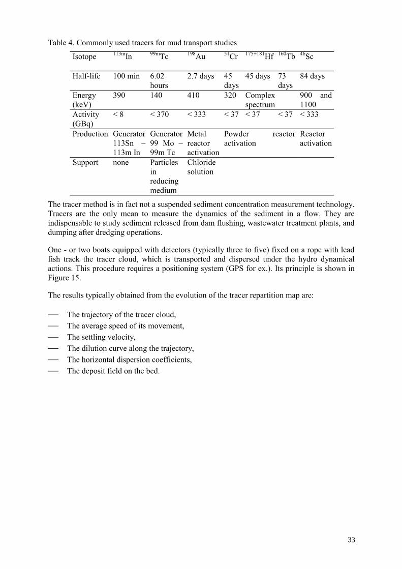
33

Table 4. Commonly used tracers for mud transport studies

Isotope 113mIn 99mTc 198Au 51Cr 175+181Hf 160Tb 46Sc

Half-life 100 min 6.02 hours

2.7 days 45 days

45 days 73 days

84 days

Energy (keV)

390 140 410 320 Complex spectrum

900 and 1100

Activity (GBq)

< 8 < 370 < 333 < 37 < 37 < 37 < 333

Production Generator 113Sn – 113m In

Generator 99 Mo – 99m Tc

Metal reactor activation

Powder reactor activation

Reactor activation

Support none Particles in reducing medium

Chloride solution

The tracer method is in fact not a suspended sediment concentration measurement technology. Tracers are the only mean to measure the dynamics of the sediment in a flow. They are indispensable to study sediment released from dam flushing, wastewater treatment plants, and dumping after dredging operations.

One - or two boats equipped with detectors (typically three to five) fixed on a rope with lead fish track the tracer cloud, which is transported and dispersed under the hydro dynamical actions. This procedure requires a positioning system (GPS for ex.). Its principle is shown in Figure 15.

The results typically obtained from the evolution of the tracer repartition map are:

The trajectory of the tracer cloud, The average speed of its movement, The settling velocity, The dilution curve along the trajectory, The horizontal dispersion coefficients, The deposit field on the bed.

33

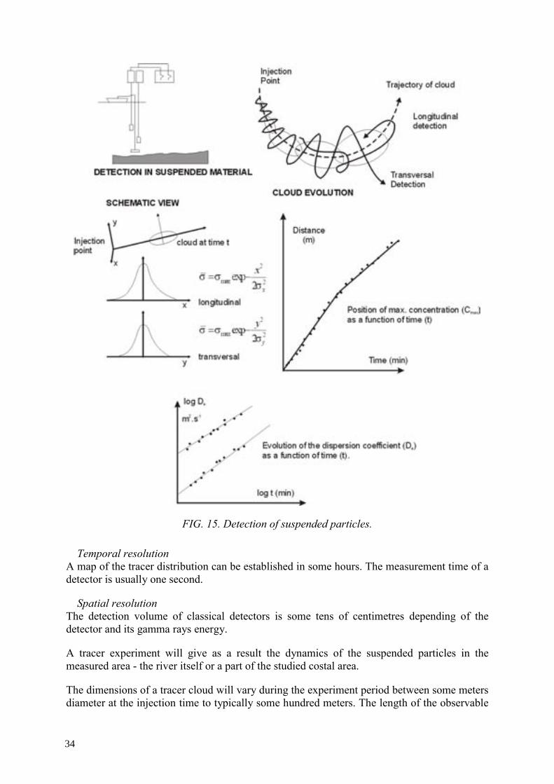
34

FIG. 15. Detection of suspended particles.

Temporal resolution A map of the tracer distribution can be established in some hours. The measurement time of a detector is usually one second.

Spatial resolution The detection volume of classical detectors is some tens of centimetres depending of the detector and its gamma rays energy.

A tracer experiment will give as a result the dynamics of the suspended particles in the measured area - the river itself or a part of the studied costal area.

The dimensions of a tracer cloud will vary during the experiment period between some meters diameter at the injection time to typically some hundred meters. The length of the observable

34

35

trajectory depends on the geometry of the site (river – 1D or 2D dispersion or see – 2D or 3D dispersion), of the size distribution of the particles and of the dispersion coefficients.

Operational ranges Not applicable. The limitation of such methodology is in the meteorological conditions but not in the measurable concentration that are very low due to the very high sensitivity of the detectors.



Accessibility The technique is applicable in any situation where the user has safe access to the water (e.g. from bridge, boat or wading). The technique can be used easily in remote places.

Power supply The power supply is depending on the accessories used:

In the simplest case, the probes are connected to a data logger (3 input channel is a minimum). The power supply is generally a simple 12V DC battery included in the data logger allowing autonomy of some days. The lead fish in this case is light (20 kg for example) and is manually operated through a simple rope. This solution can be interesting for water depth lower than 5 – 20 m.

In a more sophisticated case the probe is connected to a computer through a 12 or 24 V DC winch. In this case the lead fish can be heavier (80 kg for example) allowing access to depths greater than 10 – 50m. An external battery (car type) or a power generator will be necessary.

Manpower At least two persons are necessary; one for data acquisition and one for boat driving. It is necessary to have a person trained on safety procedures and knowledgeable on radioactivity regulation.

Regulation The use of ionizing radiation requires a clearance to be obtained from the radiological safety board and the nuclear safety authority of the country. To obtain this clearance it is necessary to present a document containing the characteristics of the experiment (nature and activity of the tracer, evaluation of tracer ingestion effect on the population). One person of the company performing the experiment will have to be trained officially to know the country regulation on ionizing radiation management and so, to be able to lead the experiment.

Maintenance Only electronic maintenance is required. The electronic cards used in the detectors are generally quite simple and rugged. Their maintenance is very simple and light. It is generally useful to check before each experiment the settings of the card and to adjust a threshold with a potentiometer (a scope will be necessary).


Data treatment (including cleaning, conversion) The raw data are classically saved into a text or Excel files as cps (counts per sec) versus time.

35

36

The first step of the data treatment is to convert time in X, Y position through data from the positioning system. This step can be performed manually by plotting on a paper map the trajectory of the boat. It can also be included in the data acquisition software or done using GIS software.

The trajectory and the average velocity of the cloud are obtained directly at this step.

The horizontal dispersion coefficients are obtained by fitting the measured concentration profiles by a Gaussian law.

The deposit field can be measured directly with a detector fixed on a sledge mapping the deposit area.

Calibration The correct exploitation of radiotracers experiment data depends on calibration undertaken in laboratory. Calibration is carried out in tanks using a radioactive source of the radionuclide, which will be used in the field with a known activity. The tank has to be big enough to place the detector in an infinite medium (1 to 2 m3 for ex.). The detector is placed at the centre of the tank and the known activity of the tracer is injected and well mixed in a known volume of water.

The calibration gives the number of counts per sec measured by the detector for 1 kBq.m-3 for example.

3. TECHNIQUES FOR MEASURING SUSPENDED SEDIMENT (UNDER DEVELOPMENT)

3.1. Acoustic (multiple frequency)

Sound of multiple frequencies (usually 3 or more, in the megahertz range) is propagated simultaneously through the water column where it is scattered from particles in suspension. Since different acoustic frequencies interact with particles of a given size in different ways, the backscatter data can be used to estimate the average size of particles in suspension. If perfected, this technique could minimize or eliminate the need to collect pump samples together with acoustic data. However, it is very difficult to convert multi-frequency backscatter data into particle sizes and concentrations. In addition, the only commercially available system (as of 2004) costs approximately $30 000 and does not include software for data conversion. This technique has successfully been applied in marine environments, but has seen little use in river environments [17], [18], [22]. This is likely due to the wider particle size and concentration ranges present in rivers. With further development this technology could become very useful. By sweeping the acoustic beam across a channel cross-section, one instrument could potentially measure particle size, particle concentration, and bathymetry in a channel cross-section (provided that the cross-section is small enough for the signal to propagate across).

3.2. Pressure differential

In this technique, the inlets of a differential pressure transducer are vertically separated by a known distance in the water column. The difference in pressure measured at the two inlets will be affected by particles suspended in the fluid between the ports. This difference can be used to infer the particle concentration. This technique has been successfully tested in the

36

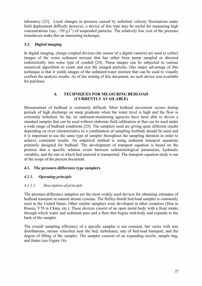
37

laboratory [23]. Local changes in pressure caused by turbulent velocity fluctuations make field deployment difficult; however, a device of this type may be useful for measuring high concentrations (say, >20 g.l-1) of suspended particles. The relatively low cost of the pressure transducers make this an interesting technique.

3.3. Digital imaging

In digital imaging, charge coupled devices (the sensor of a digital camera) are used to collect images of the water sediment mixture that has either been pump sampled or directed isokinetically into some type of conduit [24]. These images can be subjected to various numerical algorithms to count and size the imaged particles. One major advantage of this technique is that it yields images of the sediment/water mixture that can be used to visually confirm the analysis results. As of the writing of this document, no such device was available for purchase.

4. TECHNIQUES FOR MEASURING BEDLOAD (CURRENTLY AVAILABLE)

Measurement of bedload is extremely difficult. Most bedload movement occurs during periods of high discharge on steep gradients when the water level is high and the flow is extremely turbulent. So far, no sediment-monitoring agencies have been able to devise a standard sampler that can be used without elaborate field calibration or that can be used under a wide range of bedload conditions [25]. The samplers used are giving quite different results depending on river characteristics so a combination of sampling methods should be used and it is important to use the same type of sampler throughout the sampling duration in order to achieve consistent results. An empirical method is using sediment transport equations primarily designed for bedload. The development of transport equation is based on the premise that a specific relation exists between sedimentological parameters, hydraulic variables, and the rate at which bed material is transported. The transport equation study is out of the scope of the present document.

4.1. The pressure-difference type samplers



The pressure-difference samplers are the most widely used devices for obtaining estimates of bedload transport in natural stream systems. The Helley-Smith bed-load sampler is commonly used in the United States. Other similar samplers were developed in other countries (Don in Russia, Y78 in China, etc.). These devices consist of an open metal body with a front intake through which water and sediment pass and a flare that begins mid-body and expands to the back of the sampler.

The overall sampling efficiency of a specific sampler is not constant, but varies with size distributions, stream velocities near the bed, turbulence, rate of bed-load transport, and the degree of filling of the sampler. The sampler consists of an expanding nozzle, sample bag, and frame (see Figure 16).

37

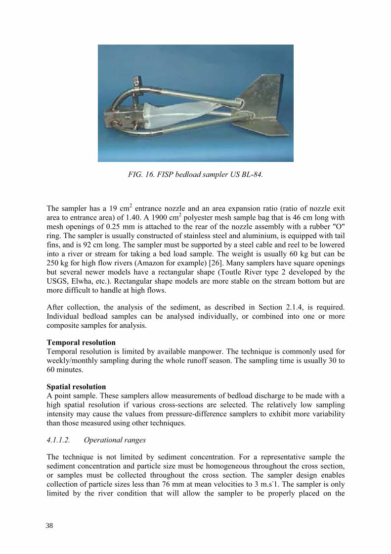
38

FIG. 16. FISP bedload sampler US BL-84.

The sampler has a 19 cm2 entrance nozzle and an area expansion ratio (ratio of nozzle exit area to entrance area) of 1.40. A 1900 cm2 polyester mesh sample bag that is 46 cm long with mesh openings of 0.25 mm is attached to the rear of the nozzle assembly with a rubber "O" ring. The sampler is usually constructed of stainless steel and aluminium, is equipped with tail fins, and is 92 cm long. The sampler must be supported by a steel cable and reel to be lowered into a river or stream for taking a bed load sample. The weight is usually 60 kg but can be 250 kg for high flow rivers (Amazon for example) [26]. Many samplers have square openings but several newer models have a rectangular shape (Toutle River type 2 developed by the USGS, Elwha, etc.). Rectangular shape models are more stable on the stream bottom but are more difficult to handle at high flows.

After collection, the analysis of the sediment, as described in Section 2.1.4, is required. Individual bedload samples can be analysed individually, or combined into one or more composite samples for analysis.

Temporal resolution Temporal resolution is limited by available manpower. The technique is commonly used for weekly/monthly sampling during the whole runoff season. The sampling time is usually 30 to 60 minutes.

Spatial resolution A point sample. These samplers allow measurements of bedload discharge to be made with a high spatial resolution if various cross-sections are selected. The relatively low sampling intensity may cause the values from pressure-difference samplers to exhibit more variability than those measured using other techniques.


The technique is not limited by sediment concentration. For a representative sample the sediment concentration and particle size must be homogeneous throughout the cross section, or samples must be collected throughout the cross section. The sampler design enables collection of particle sizes less than 76 mm at mean velocities to 3 m.s-1. The sampler is only limited by the river condition that will allow the sampler to be properly placed on the

38

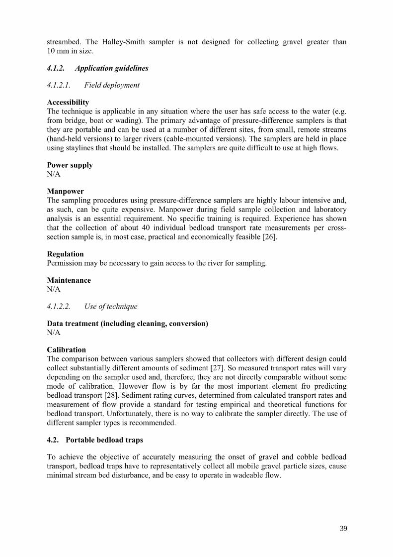
39

streambed. The Halley-Smith sampler is not designed for collecting gravel greater than 10 mm in size.



Accessibility The technique is applicable in any situation where the user has safe access to the water (e.g. from bridge, boat or wading). The primary advantage of pressure-difference samplers is that they are portable and can be used at a number of different sites, from small, remote streams (hand-held versions) to larger rivers (cable-mounted versions). The samplers are held in place using staylines that should be installed. The samplers are quite difficult to use at high flows.

Power supply N/A

Manpower The sampling procedures using pressure-difference samplers are highly labour intensive and, as such, can be quite expensive. Manpower during field sample collection and laboratory analysis is an essential requirement. No specific training is required. Experience has shown that the collection of about 40 individual bedload transport rate measurements per cross-section sample is, in most case, practical and economically feasible [26].


Maintenance N/A


Data treatment (including cleaning, conversion) N/A

Calibration The comparison between various samplers showed that collectors with different design could collect substantially different amounts of sediment [27]. So measured transport rates will vary depending on the sampler used and, therefore, they are not directly comparable without some mode of calibration. However flow is by far the most important element fro predicting bedload transport [28]. Sediment rating curves, determined from calculated transport rates and measurement of flow provide a standard for testing empirical and theoretical functions for bedload transport. Unfortunately, there is no way to calibrate the sampler directly. The use of different sampler types is recommended.

4.2. Portable bedload traps

To achieve the objective of accurately measuring the onset of gravel and cobble bedload transport, bedload traps have to representatively collect all mobile gravel particle sizes, cause minimal stream bed disturbance, and be easy to operate in wadeable flow.

39

40



The prominent characteristics of the bedload sampling device are a large opening and a long sampling time-attributes more typical of a ‘‘trap’’ than a ‘‘sampler.’’ The term ‘‘bedload trap’’ is therefore used to describe these devices, even though they are not installed below the bed surface.

The bedload traps have a sturdy aluminum frame 0.3 m wide, 0.2 m high, and 0.1 m deep. Dimensions were selected to accommodate particles up to small cobble sizes (approximately 128 mm). In the field, the frame is placed onto a ground plate to ensure good contact with the stream bottom. The front edge of the ground plate is inclined down in the upstream direction to provide a smooth transition between the streambed and the trap entrance. Sediment is collected in a trailing net that extends approximately 1 m downstream of the frame [29].

Fig. 17. Schema of the bed load trap developed by Bunte and Potyondy [29].

After collection, the analysis of the sediment, as described in Section 2.1.4, is required.

Temporal resolution Typically one-hour sampling period

Spatial resolution One or various traps could be installed. Traps are best installed at a wide riffle since this is the most wadeable part of the stream and provides the best chances for servicing traps during high flow. The combined widths of all traps installed across the stream should cover 20–40% of the active streambed, depending on the desired sampling intensity or accuracy with respect to lateral variability of bedload transport.

40

41


The technique is not limited by sediment concentration. For a representative sample the sediment concentration and particle size must be homogeneous throughout the cross section, or samples must be collected throughout the cross section. Portable trap operation is limited to flows in which an operator can reach down to the stream bottom to empty the traps. The traps are not suitable for collecting particles smaller than 4 mm.



Accessibility Bedload trap installation is best done at relatively low flows, a few days prior to the onset of bedload transporting flows. A small area of the streambed is cleared of large surface particles to obtain a level space onto which the ground plate flush is positioned with the average height of the streambed. The traps are fixed in the river in order to insure a good contact with the stream bottom.

Manpower No more than two persons are necessary. One should be available to empty the traps.

Regulation The traps are interfering flow and therefore it is important to insure that no boat is passing during the measurement period.

Maintenance N/A



Calibration N/A

4.3. Permanent traps



A trap is build preferably across the entire width of the stream. Openings of the trap should be larger than the maximum hop length of saltation particles. The material accumulates in an inner container that periodically requires emptying.

Various systems were developed; the conveyor belt slot system, the Vortex tube system, the weighing slot (pit) sampler system, and the Birkbeck-type automatic monitoring slot sampler. The systems are semi-automatic or automatics.

41

42

A vortex bedload sampler includes a flume, rectangular weir, off-channel sampling pit, and a bypass flume. By opening flow gates, the flume created a vortex and extracted bed load from the stream so that transport rates could be measured.

The Birkbeck bed load sampler weighs the mass of bed load that enters a slot. It has become the preferred method for bed load transport estimation.

Temporal resolution This method allows the continuous measurement of the bedload transport.

Spatial resolution Cross-section of the river.


The technique is not limited by sediment concentration. For a representative sample the sediment concentration and particle size must be homogeneous throughout the cross section, or samples must be collected throughout the cross section. The technique is usually used in perennial or seasonal streams when the flow is predictable. Trap operation is limited to flows in which an operator can reach down to the stream to empty the traps.

Pit traps have variable efficiency. During high flow, sand and fine gravel in suspension and even mid-sized gravel particles may skip over the trap opening. There is an under-prediction of transport rates at high flows. Traps are not sensitive to the effects of varying direction of the oncoming current. During highest flow the upper limit of grain sizes to be relented from the sampler is 3–16mm. Trap efficiency begins to decline at approximately 3–4 mm.



Accessibility Small non-recording pit trap samplers can be installed in a streambed by a small field crew with shovels and buckets. However, trap operation is limited to flows in which an operator can reach down to the stream bottom to empty the traps. Pit traps also have highly variable sampling efficiencies. During high flow, sand and fine gravel may travel in suspension and even mid-sized gravel particles may skip over the trap opening.

Manpower For such system, substantial streambed construction is involved in the installation, which makes these devices difficult, time-consuming, costly to deploy.

Regulation Need authorization to build the sampler across the river.

Maintenance Emptying the container regularly (the frequency depends on the river and transport characteristics).



42

43

Calibration Calibration regression equations should be loaded regularly. Sampler calibration varied, often by about 5% between years.

4.4. Nuclear gauges



For such application, both principles described in Section 2.3 can be used. The system is measuring the variations of the thickness of the moving layer. To quantify the sediment transport the movement has to be with sedimentary forms (dunes, riddens, etc). It is not possible to measure anything if the bed is flat.

The most common system is the transmission one shown in Figure 17.

The second system possible to use for bedload transport determination is a scattering system (Figure 8).

FIG. 18. Principles of nuclear transmission for bedload transport determination.

FIG. 19. Principles of nuclear scattering system.

43

44

The transmission system is simpler and more sensitive than for the scattering one because the energy of the emitted photons can be lower.

Basically the transmission system is using an Iridium-192 source (half-life 74 days, energy between 300 and 468 keV) or a Caesium-137 source (half-life 30 years but use limited to 10 years by the regulation, energy 662 keV). For the scattering system it is necessary to use a Cobalt-60 source (half-life 5.27 years, energy 1173 and 1332 keV) with some additional safety constraints. The main interest of the scattering system is that all the system is buried into the sand bed, so there are fewer security problems.

Temporal resolution The temporal resolution is the same as for the systems presented in Section 2.3. The dwell time has to be adapted to the speed of the moving sedimentary forms.

Spatial resolution See Section 2.3.


This type of system can typically measure thickness variations from 1 to 30 cm.



Accessibility The technique is applicable in any situation where the user has safe access to the water (e.g. from bridge, boat or wading). Can be used easily in remote places.

These systems have to be installed in the sediment bed. It is therefore necessary to work with divers or better, to install the system during low water level.

Power supply See Section 2.3.

Manpower See Section 2.3.

Maintenance See Section 2.3.


See Section 2.3.

4.5. Tracer techniques



See Section 2.3. The pebbles are individually labelled with 192Ir, 182Ta or 110mAg wires. The total number of pebbles is normally restricted to about 1000 per site due to this time-consuming procedure.

44

45

The tracer method is an integrating method. The tracer (and the traced sediment) is supporting all the hydrodynamical actions imposed by the water motion. The measurement is the resultant of all these actions between two periods of time.

Quantitative measurement of transport of bed load sediment by tracers can be founded mainly on procedures that are conceptually Lagrangian.

A boat with a detector on a sledge produces a map of the tracer repartition (Figure 21). This procedure requires a positioning system (e.g. GPS ). Its principle is shown in Figure 20.

FIG. 20. Principles of the tracing methods for quantitative measurement of transport of bed load sediment.

The results typically obtained from the evolution of the tracer repartition map are:

The direction of the sediment motion, The average speed of its movement, The thickness of the moving layer, The sediment load.

Temporal resolution A map of the tracer repartition has to be established after each significant meteorological event, that means from every day to every month depending on the objectives of the study, the site and events.

Spatial resolution The detection volume of classical detectors is some tens of centimetres depending of the detector itself and of the gamma rays energy.

A tracer experiment will give as result the bed load in the measured area i.e. the river itself or a part of the studied costal area. The dimensions of a tracer cloud will vary during the experiment period between some meters diameter at the injection time to ~500 m width and 2–3 km long.

45

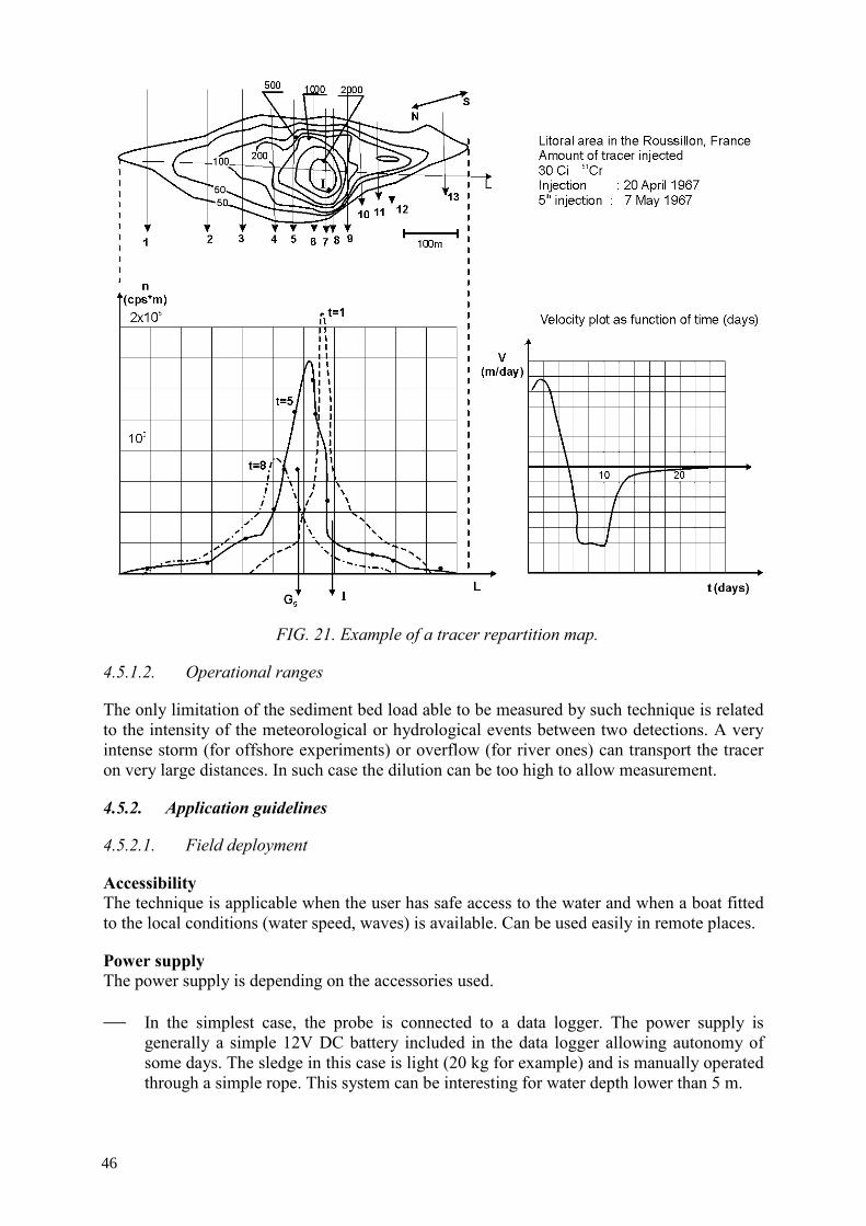
46

FIG. 21. Example of a tracer repartition map.


The only limitation of the sediment bed load able to be measured by such technique is related to the intensity of the meteorological or hydrological events between two detections. A very intense storm (for offshore experiments) or overflow (for river ones) can transport the tracer on very large distances. In such case the dilution can be too high to allow measurement.



Accessibility The technique is applicable when the user has safe access to the water and when a boat fitted to the local conditions (water speed, waves) is available. Can be used easily in remote places.

Power supply The power supply is depending on the accessories used.

In the simplest case, the probe is connected to a data logger. The power supply is generally a simple 12V DC battery included in the data logger allowing autonomy of some days. The sledge in this case is light (20 kg for example) and is manually operated through a simple rope. This system can be interesting for water depth lower than 5 m.

46

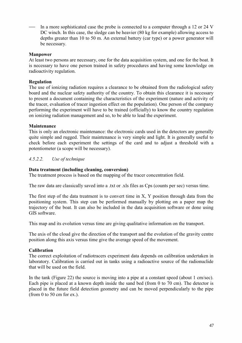
47

In a more sophisticated case the probe is connected to a computer through a 12 or 24 V DC winch. In this case, the sledge can be heavier (80 kg for example) allowing access to depths greater than 10 to 50 m. An external battery (car type) or a power generator will be necessary.

Manpower At least two persons are necessary, one for the data acquisition system, and one for the boat. It is necessary to have one person trained in safety procedures and having some knowledge on radioactivity regulation.

Regulation The use of ionizing radiation requires a clearance to be obtained from the radiological safety board and the nuclear safety authority of the country. To obtain this clearance it is necessary to present a document containing the characteristics of the experiment (nature and activity of the tracer, evaluation of tracer ingestion effect on the population). One person of the company performing the experiment will have to be trained (officially) to know the country regulation on ionizing radiation management and so, to be able to lead the experiment.

Maintenance This is only an electronic maintenance: the electronic cards used in the detectors are generally quite simple and rugged. Their maintenance is very simple and light. It is generally useful to check before each experiment the settings of the card and to adjust a threshold with a potentiometer (a scope will be necessary).


Data treatment (including cleaning, conversion) The treatment process is based on the mapping of the tracer concentration field.

The raw data are classically saved into a .txt or .xls files as Cps (counts per sec) versus time.

The first step of the data treatment is to convert time in X, Y position through data from the positioning system. This step can be performed manually by plotting on a paper map the trajectory of the boat. It can also be included in the data acquisition software or done using GIS software.

This map and its evolution versus time are giving qualitative information on the transport.

The axis of the cloud give the direction of the transport and the evolution of the gravity centre position along this axis versus time give the average speed of the movement.

Calibration The correct exploitation of radiotracers experiment data depends on calibration undertaken in laboratory. Calibration is carried out in tanks using a radioactive source of the radionuclide that will be used on the field.

In the tank (Figure 22) the source is moving into a pipe at a constant speed (about 1 cm/sec). Each pipe is placed at a known depth inside the sand bed (from 0 to 70 cm). The detector is placed in the future field detection geometry and can be moved perpendicularly to the pipe (from 0 to 50 cm for ex.).

47

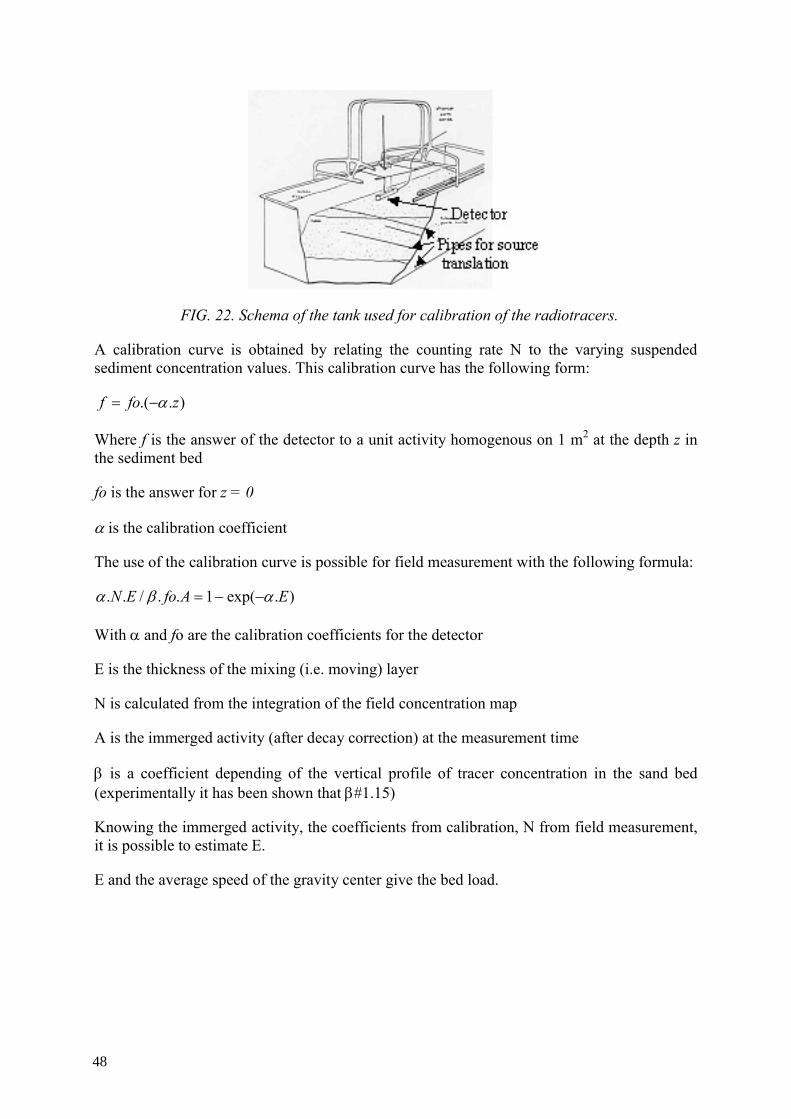
48

FIG. 22. Schema of the tank used for calibration of the radiotracers.

A calibration curve is obtained by relating the counting rate N to the varying suspended sediment concentration values. This calibration curve has the following form:

)..( zfof α−=

Where f is the answer of the detector to a unit activity homogenous on 1 m2 at the depth z in the sediment bed

fo is the answer for z = 0

α is the calibration coefficient

The use of the calibration curve is possible for field measurement with the following formula:

).exp(1../.. EAfoEN αβα −−=

With α and fo are the calibration coefficients for the detector

E is the thickness of the mixing (i.e. moving) layer

N is calculated from the integration of the field concentration map

A is the immerged activity (after decay correction) at the measurement time

β is a coefficient depending of the vertical profile of tracer concentration in the sand bed (experimentally it has been shown that β#1.15)

Knowing the immerged activity, the coefficients from calibration, N from field measurement, it is possible to estimate E.

E and the average speed of the gravity center give the bed load.

48

49

5. TECHNIQUES FOR MEASURING BEDLOAD (UNDER DEVELOPMENT)

5.1. Passive acoustic

Sound generated by particle impacts is employed for detecting bedload movement. The non-invasive acoustic system allows the measurement of spatially integrated bedload transport rates. The system consists of hydrophones and geophones deployed along a reach, with data recorded to disk after signal conversion. The phones are installed onto the bedrocks near the banks and onto large boulders in the centre of the stream.

The sensor record acoustic energy of bedload impact on a plate fixed to the river bad.

It is necessary to eliminate signals from fluid turbulence, cavitation, and bubble collapse. The remaining signal is integrated over a period of one second and the amplitude of the value output in digital form as a numeric string. The system should be calibrated using bedload transport rates observed at low flows by conventional techniques.

This new system should allow measurement cross-sectionally-integrated at very short time intervals. It allows monitoring temporal variations in bedload transport and thereby provides additional information about the transport process.

All electronics components have to be mounted in a robust and watertight stainless steel housing.

The results obtained using this technique are showing a good relation with classical methods. The system must be calibrated to direct samples of bedload for each measuring sites. The system allows monitoring temporal variations in the rate of bed load transport where classical methods fail to capture the episodic high flux rates [30]. The method shows also potential for use in stream channels with gravel beds. Up to know few quantitative analyses have been performed using passive acoustic system. It is not an expensive method.

5.2. Sonar imaging

The rate of sediment transport per unit width represented by a migrating bedform, called the bedform transport rate” is equal to the product of three terms: bedform height, bedform migration speed, and a dimensionless shape factor. These values can be measured easily in laboratories but not in the field. The bedload rates measured using this approach are mean rates of the area over which bedform heights and migration rates are sampled. Rotating side-sonar is well suited for field observations of bedform migration. It scans circular areas of bed. Modern commercially available systems are digital and weigh just a few kilos.

Sequential images at a site are converted into digital movies and displayed on a computer system. Individual dunes and their migration speeds can be determined.

Rotating side-scan sonar system measurements does not involved direct contact with the river bed. The method allows accurate measurements of bedload transports [31].

5.3. Impact sensors

The instrument permit to detect the acceleration of a steel plate fixed to a rock river bed. A counting data logger is attached to the underside of this plate within a recess chiselled into the bedrock. The steel plate is fixed to the bedrock. The acceleration sensor is placed within the water-tight data logger and uses the same battery supply. The system should be installed

49

50

during low-water conditions but allows measurement during high-flows also. The system is not sensitive to clast-size. The detection threshold has to be calibrated. It permits detection of particles of few mm. The device is small and very robust and can be deployed in high-energy bedrock channels. The cost of the field unit is around $750. There are some constraints not yet solved; the sensor can record only 3 counts max. per second and impacts which occurs less than 1/3 second after the previous one are not recorded [32].

6. CONCLUSIONS

Many options exist for the measurement of suspended sediment in rivers. A summary of the information collected and described within this document is given in Table 5 for methods used in determination of suspended sediment measurements and in Table 6 for the methods used for bedload determination. The in-river equipment includes the cost of sensor heads and/or sample bottles. Associated equipment includes the cost of all on-site equipment other than that in the stream (e.g. data loggers). Laboratory equipment includes the cost of basic laboratory gear necessary to analyse associated physical samples. The final decision would depend on budget constraints, manpower, desired quality of data, etc. It is highly recommended, if possible, to use more than one technique in order to obtain independent results.

50

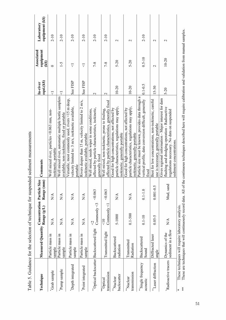
Tabl

e 5.

Gui

danc

e fo

r the

sele

ctio

n of

tech

niqu

e fo

r sus

pend

ed se

dim

ent m

easu

rem

ents

Tec

hniq

ue

Mea

sure

d Q

uant

ityC

once

ntra

tion

Ran

ge (g

/L)

Part

icle

Siz

e R

ange

(mm

)C

omm

ents

In

-riv

er

equi

.(k$)

A

ssoc

iate

d eq

uipm

ent

(k$)

L

abor

ator

y eq

uipm

ent (

k$)

* Gra

b sa

mpl

e Pa

rticl

e m

ass i

n sa

mpl

e N

/A

N/A

W

ell m

ixed

rive

r, pa

rticl

es <

0.06

3 m

m, n

on-

isok

inet

ic, p

orta

ble

<1

0 2-

10

* Pum

p sa

mpl

e Pa

rticl

e m

ass i

n sa

mpl

e N

/A

N/A

W

ell m

ixed

rive

r, au

tom

atic

mul

tiple

bot

tle sa

mpl

ers

avai

labl

e, n

on-is

okin

etic

, fix

ed o

r por

tabl

e <1

1-

5 2-

10

* Dep

th in

tegr

ated

Pa

rticl

e m

ass i

n sa

mpl

e N

/A

N/A

V

ersa

tile,

mos

t com

mon

ly u

sed,

rive

rs <

15 m

dee

p,

velo

city

lim

ited

to: 3

m/s

, iso

kine

tic a

vaila

ble,

po

rtabl

e Se

e FI

SP

<1

2-10

* Poin

t int

egra

ted

Parti

cle

mas

s in

sam

ple

N/A

N

/A

Riv

ers d

eepe

r tha

n 15

m, v

eloc

ity li

mite

d to

2 m

/s,

isok

inet

ic a

vaila

ble,

por

tabl

e Se

e FI

SP

<1

2-10

**O

ptic

al b

acks

catte

rB

acks

catte

red

light

<2

C

omm

only

<3

<0.0

63

Wel

l mix

ed, n

eeds

wip

er in

som

e co

nditi

ons,

affe

cted

by

parti

cle

char

acte

ristic

s, is

okin

etic

, ge

nera

lly fi

xed

2 7-

8 2-

10

**O

ptic

al

trans

mis

sion

Tr

ansm

itted

ligh

t <1

0 C

omm

only

<1

<0.0

63

Wel

l mix

ed, n

on-is

okin

etic

, pro

ne to

foul

ing,

af

fect

ed b

y pa

rticl

e ch

arac

teris

tics,

gene

rally

fixe

d 2

7-8

2-10

**

Nuc

lear

ba

cksc

atte

r B

acks

catte

red

radi

atio

n 5-

1000

N

/A

Goo

d fo

r hig

h co

ncen

tratio

ns, n

ot a

ffec

ted

by

parti

cle

char

acte

ristic

s, re

gula

tions

may

app

ly,

isok

inet

ic, g

ener

ally

por

tabl

e 10

-20

5-20

2

**N

ucle

ar

trans

mis

sion

Tr

ansm

itted

R

adia

tion

0.1-

500

N/A

G

ood

for h

igh

conc

entra

tions

, not

aff

ecte

d by

pa

rticl

e ch

arac

teris

tics,

regu

latio

ns m

ay a

pply

, is

okin

etic

, gen

eral

ly p

orta

ble

10-2

0 5-

20

2

**Si

ngle

freq

uenc

y ac

oust

ic

Bac

ksca

ttere

d So

und

0.1-

10

0.1-

1.0

Parti

cle

size

mus

t be

know

n, p

rovi

des d

ata

thro

ugh

a ve

rtica

l pro

file,

dat

a co

nver

sion

diff

icul

t, ge

nera

lly

fixed

0.

1-0.

5 0.

5-10

2-

10

**La

ser d

iffra

ctio

n D

iffra

cted

lase

r an

gle

0.05

-5

0.00

1-0.

5 B

est f

or lo

w c

once

ntra

tions

, non

-isok

inet

ic, c

aref

ul

use

is n

eces

sary

, gen

eral

ly p

orta

ble

15-3

0 2

2

* Rad

ioac

tive

trace

rs

Dyn

amic

s of t

he

sedi

men

t in

a flo

w

N/A

M

ud, s

and

Giv

es re

gion

al in

form

atio

n - M

ajor

inte

rest

for d

am

flush

ing

and

dred

ging

ope

ratio

n - R

adio

activ

e re

gula

tions

nec

essa

ry. N

o da

ta o

n su

spen

ded

sedi

men

t con

cent

ratio

ns.

5-20

10

-20

2

*

Thes

e te

chni

ques

will

requ

ire la

bora

tory

ana

lysi

s. **

Th

ese

are

tech

niqu

es th

at w

ill c

ontin

uous

ly re

cord

dat

a. A

ll of

the

cont

inuo

us te

chni

ques

des

crib

ed h

ere

will

requ

ire c

alib

ratio

n an

d va

lidat

ion

from

man

ual s

ampl

es.

51

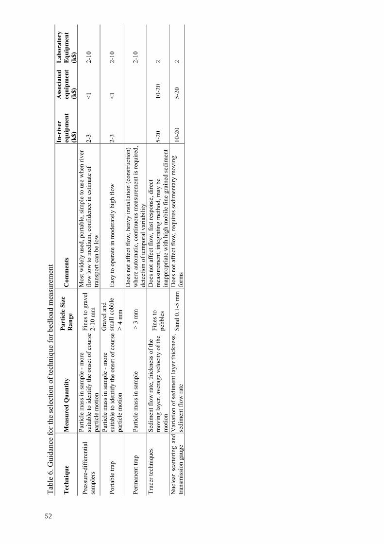
Tabl

e 6.

Gui

danc

e fo

r the

sele

ctio

n of

tech

niqu

e fo

r bed

load

mea

sure

men

t

Tec

hniq

ue

Mea

sure

d Q

uant

ity

Part

icle

Siz

e R

ange

C

omm

ents

In

-riv

er

equi

pmen

t (k

$)

Ass

ocia

ted

equi

pmen

t (k

$)

Lab

orat

ory

Equ

ipm

ent

(k$)

Pr

essu

re-d

iffer

entia

l sa

mpl

ers

Parti

cle

mas

s in

sam

ple

- mor

e su

itabl

e to

iden

tify

the

onse

t of c

ours

e pa

rticl

e m

otio

n Fi

nes t

o gr

avel

2-

10 m

m

Mos

t wid

ely

used

, por

tabl

e, si

mpl

e to

use

whe

n riv

er

flow

low

to m

ediu

m, c

onfid

ence

in e

stim

ate

of

trans

port

can

be lo

w

2-3

<1

2-10

Porta

ble

trap

Parti

cle

mas

s in

sam

ple

- mor

e su

itabl

e to

iden

tify

the

onse

t of c

ours

e pa

rticl

e m

otio

n

Gra

vel a

nd

smal

l cob

ble

> 4

mm

Ea

sy to

ope

rate

in m

oder

atel

y hi

gh fl

ow

2-3

<1

2-10

Perm

anen

t tra

p Pa

rticl

e m

ass i

n sa

mpl

e >

3 m

m

Doe

s not

aff

ect f

low

, hea

vy in

stal

latio

n (c

onst

ruct

ion)

w

here

aut

omat

ic, c

ontin

uous

mea

sure

men

t is r

equi

red,

de

tect

ion

of te

mpo

ral v

aria

bilit

y

2-

10

Trac

er te

chni

ques

Se

dim

ent f

low

rate

, thi

ckne

ss o

f the

m

ovin

g la

yer,

aver

age

velo

city

of t

he

mot

ion

Fine

s to

pebb

les

Doe

s not

aff

ect f

low

, fas

t res

pons

e, d

irect

m

easu

rem

ent,

inte

grat

ing

met

hod,

may

be

inap

prop

riate

with

hig

h m

obile

fine

gra

ined

sedi

men

t 5-

20

10-2

0 2

Nuc

lear

sca

tterin

g an

d tra

nsm

issi

on g

auge

V

aria

tion

of se

dim

ent l

ayer

thic

knes

s, se

dim

ent f

low

rate

Sa

nd 0

.1-5

mm

Doe

s not

aff

ect f

low

, req

uire

s sed

imen

tary

mov

ing

form

s 10

-20

5-20

2

52

53

REFERENCES

[1] Department of the Army, Office of the Chief of Engineers, Engineering, and Design - Sedimentation Investigations of Rivers and Reservoirs. Report EM 1110-2-4000 (1995).

[2] Old, G.H., Leeks, G.J.L., Packman, J.C.P., Smith, B.P.G., Lewis, S., Hewitt, E. J., Holmes M., Young, A., The impact of a convectional summer rainfall event on river flow and fine sediment transport in a highly urbanised catchment: Bradford, West Yorkshire. Science of the Total Environment. 314–316 (2003) 495–512.

[3] Wren, D.G., Barkdoll, B.D., Kuhnle, R.A., Derrow, R.W, Field techniques for suspended-sediment measurement, Journal of Hydraulic Engineering (2000), 97–104.

[4] Old, G.H., Leeks, G.J.L., Cooper, D., McNeil, D., Evans, J., Hodgson, P., Smith, P. and Proctor, J., Two technological advances in continuous monitoring of suspended sediment transport and particle characteristics. In Erosion and Sediment Transport Measurement in Rivers: Technological and Methodological Advances. J. Bogen, T. Fergus and D. Walling (Eds) Volume of Extended Abstracts from the International Workshop in Oslo: Norway 19–21 June 2002, IAHS Publication, Wallingford.

[5] Federal Interagency Sedimentation Project (FISP), The US-D96: An isokinetic suspended sediment /water quality collapsible bag-sampler. Internal Report (2001) 41 pp.

[6] ASTM, Standard Test Methods for Determining Sediment Concentration in Water Samples. ASTM D3977-97 (2002).

[7] Department of the Army, Office of the chief of Engineers, Engineering and Design - Laboratory Soil testing. Report EM 1110-2-1906 (1970).

[8] American Society of Civil Engineers (ASCE), Sedimentation Engineering, American Society of Civil Engineering, Manual No 54, V. Vanoni Ed., New York, USA (1975).

[9] Gippel, C.J., The use of turbidimeters in suspended sediment research, Hydrobiologia, 176/177, (1989) 465–480.

[10] Ludwig, K.A., Hanes, D.M., A laboratory evaluation of optical backscatterance suspended solids sensors exposed to sand-mud mixture. Marine Geology, 94 (1990) 173–179.

[11] Conner, C.S., DeVisser, A.M., A laboratory investigation of particle size effects on an optical backscatterance sensor, Marine Geology, 10 (1992) 151–159

[12] Hay, A.E., On the remote acoustic detection of suspended sediment at long wavelengths. Journal of Geophysical Research. 88(C12) (1983) 7525–7542.

[13] Thorne, P.D.; Hardcastle, P.J., Soulsby, R.L., Analysis of Acoustic Measurements of Suspended Sediments. Journal of Geophysical Research, 98-C1, (1993) 899–910.

[14] Thorne, P.D.; Hardcastle, P.J.; Flatt, D., Humphery, J.D., On the use of acoustics for measuring shallow water suspended sediment processes. IEEE Journal of Oceanic Engineering. 19(1) (1994) 48–57.

[15] Sheng, J., and A. E. Hay, Spherical wave backscatter from cylinders: thin-wire standard targets, J. Acoustic Soc. Am., 94, 2756–2765 (1993).

[16] Lee, T.H., Hanes, D.M., Direct inversion method to measure the concentration profile of suspended particles using backscattered sound. Journal of Geophysical Research. 100(C2) (1995) 2649–2657

53

54

[17] Hay, A.E., Sheng, J., Vertical Profiles of Suspended Sand Concentration and Size from Multifrequency Acoustic Backscatter. Journal of Geophysical Research. 97(C10) (1992) 15661–15677.

[18] Crawford, A. M., Hay, A.E., Determining suspended sand size and concentration from multifrequency acoustic backscatter. The Journal of the Acoustical Society of America. 94(6) (1993) 3312–3324.

[19] Urick, R.J., Principles of Underwater Sound. 3rd ed. Los Altos, California: Peninsula Publishing (1983).

[20] Melis, T.S., Topping, D.J., Rubin, D.M., Testing laser-based sensors for continuous in situ monitoring of suspended sediment in the Colorado River, Arizona, Erosion and Sediment transport Measurement in Rivers: technological and Methodological Advances - Proceedings of the Oslo Workshop, June 2002, IAHS Publication 283 (2003).

[21] Agrawal, Y.C., Pottsmith, H.C., Laser instrument for particle sizing and settling velocity measurements in the coastal zone. Proceedings Oceans-Conference, 1996 - Vol. I, IEEE, Piscataway, N.J., (1996). 1135–1142

[22] Thorne, P.D., Hardcastle, P.J., Acoustic measurements of suspended sediments in turbulent currents and comparison with in situ samples. The Journal of the Acoustical Society of America. 101(5) (1997) 2603–2614.

[23] Lewis, A. J., Rasmussen, T. C., A New, Passive Technique for the In Situ Measurement of Total Suspended Solids Concentrations in Surface Water. Technical Completion Report for project # 14-08-001-G-2013 (07), U.S. Department of the Interior, Geological Survey (1996).

[24] Gooding, D. J., Photo Optical Sedimentation Tube. Poster-29 Federal Interagency Sedimentation Conference in Reno, Nevada (2001).

[25] UNEP/WMO, Water Quality Monitoring - A practical Guide to the Design and Implementation of Freshwater Quality Studies and Monitoring Programmes. Chap.13: Sediment measurements, UNEP (1996) 184p.

[26] Edwards, T.K., Glysson, G.D., Field methods for measurement of fluvial sediment. In: Book 3, Application and Hydraulics. Chapter C2. USGS manual (1999) 89 p.

[27] Hubbell, D.W., Stevens, H.H., Skinner, J.V., beverage, J.P., Recent refinements in calibrating bedload samplers. In: Water forum ’81. American Society of Civil Engineers, New-York, 1 (1981) 128–140.

[28] Ryan, S.E., The use of pressure-difference samplers in measuring bedload transport in small, coarse grained alluvial channels. http://water.usgs.gov/osw/techniques/sediment/sedsurrogate2003workshop/Flagstaff_Bedload_2003.pdf.

[29] Bunte, K., Potyondy, J., A Bedload Trap for Sampling Coarse Gravel and Cobble Transport in Wadeable Mountain Streams. Stream Note of the Rocky Mountain Research Station, October 2004.

[30] Downing, J., Farley, P.J., Bunte, K., Swingle, K., Ryan, S.E., Dixon, M., Acoustic gravel-trasnport sensor: description and filed tests in Little Granite Creek, Wyoming, USA. In: Erosion and Sediment Transport Measurement in Rivers: Technological and Methodological Advances, Proceedings of the Oslo workshop, June 2002, IAHS Publ. 283 (2003).

[31] Rubin, D.M., Tate, G.B., Topping, D.J., Anima, R.A., Use of rotating side-scan sonar to measure bedload. In: Proceedings of the Seventh Federal Interagency Sedimentation Conference, Reno, USA, pp. III (2001) 139–144.

54

55

[32] Richardson, K., Benson, I., Carling P.A., An instrument to record sediment movement in bedrock channels in: Erosion and Sediment Transport Measurement in Rivers: Technological and Methodological Advances (Proceedings of the Oslo Workshop, June 2002). IAHS Publication 283 (2002) p. 228–235

55

56

BIBLIOGRAPHY

General literature and Web Sites IAHS #283, Erosion and Sediment Transport Measurement in Rivers: Technological and Methodological Advances.

http://fisp.wes.army.mil/

http://water.usgs.gov/osw/techniques/sedimentpubs.html

Manual sampling and concentration determination Evans, J.G., P.D. Wass, P. Hodgson, 1997: Integrated continuous water quality monitoring for the LOIS rivers programme. Science of the Total Environment, 194/195:111–118.

Foster, IDL, Millington R, Grew RG. 1992. The impact of particle size controls on stream turbidity measurement; some implications for suspended sediment yield estimation. Int. Assoc. Hydrol. Sci., 201:51–62.

Gippel, C.J. 1995. Potential of turbidity monitoring for measuring the transport of suspended solids in streams. Hydrological Processes, 9:83–97.

Lawler D M, 1995: Turbidity and Nephelometry. Encyclopedia of Analytical Science, 9:5289–5297.

Lawler, D.M., Brown, R.M. 1992: A simple and inexpensive turbidity meter for the estimation of suspended sediment concentrations. Hydrological Processes, 6:159–168.

Lewis, J. 1996: Turbidity-controlled suspended sediment sampling for runoff-event load estimation. Water Resources Research, 32 (7):2299–2310.

Syvitski, James P., 1991: Principles, Methods, and Application of Particle Size Analysis, Cambridge University Press, Cambridge, U.K.

Wass P. D., Marks S. D., Finch J. W., Leeks G. J. L. L., Ingram J. K., 1997: Monitoring and preliminary interpretation of in-river turbidity and remote sensed imagery for suspended sediment transport studies in the Humber catchment. Science of the Total Environment. 194/195:263–283

Wass, P.D., G.J.L. Leeks, 1999: Suspended sediment fluxes in the Humber catchment, UK. Hydrological Processes, 13:935–953.

Single Frequency Acoustic Suspended-Sediment measurement

Crawford, A. M., Hay, A.E. 1993: Determining suspended sand size and concentration from multifrequency acoustic backscatter. The Journal of the Acoustical Society of America. 94(6):3312–3324.

He, C., Hay, A.E. 1993: Broadband Measurements of the Acoustic Backscatter Cross Section of Sand Particles in Suspension. Journal of the Acoustical Society of America. 94(4):2247–2254.

Thorne, P.D.; Hardcastle, P.J., Soulsby, R.L. 1993: Analysis of Acoustic Measurements of Suspended Sediments. Journal of Geophysical Research, 98(C1):899–910.

57

57

Thorne, P.D.; Hardcastle, P.J.; Flatt, D., Humphery, J.D. 1994: On the use of acoustics for measuring shallow water suspended sediment processes. IEEE Journal of Oceanic Engineering. 19(1): 48–57.

Nuclear techniques Brisset, P., Hoslin, R., Meyer, G., Caillot, A. 1996: Study and optimisation of dredging works using radioactivity-The case of zeebrugge harbour. IAEA-SM-223/8.

Brisset, P., Vabre, A., Poggi, A. 2000: Les apports de l'instrumentation nucléonique et des traceurs à la sédimentologie dynamique. Sixièmes journées nationales Génie civil - Génie Côtier. Caen 17–19 mai 2000. ISBN 2-9505787-5-6.

Caillot A., Courtois G., Quesney M., Sauzay G. 1976: Theoretical approach of transport by suspension. in: Method of analysis of radioactive tracers measures. Study of sea gravels (vol. 2) CEA internal report SAR – CNEXO (in French).

Crickmore, M.J., Tazioli, G.S., Appleby. P.G., Oldfield, F., 1990: The use of nuclear techniques in sediment transport and sedimentation problems. Technical Documents in Hydrology, SC-90/WS-49, Unesco, Paris.

Csanady G.T. 1973: Turbulent diffusion in the environment. D.Reidel. Publishing: Company Dordrecht, Holland.

IAEA, 1962: Application of Isotope Techniques in Hydrology, STI/DOC/10/11. A comprehensive report from the panel held in Vienna, 6–9 November 1962. 31 pages.

IAEA, 1967: Isotopes in Hydrology. Proceedings of a symposium held in Vienna, November 13–18, 1966. STI/PUB/141, Vienna, 740 pages.

IAEA, 1973: Tracer Techniques in Sediment Transport. Proceedings of the Panel Meeting held in Saclay, France, June 21–25, 1971. STI/DOC/10/145, Vienna, 234 pages.

IAEA, 1983: Radioisotopes in Sediment Studies. Report of a Consultants' Meeting held in Vienna, 13–17 December 1982. IAEA-TECDOC-298, Vienna, 75 pages.

Sauzay G. The ‘’count rate balance’’ method for measuring sediment transport of sand beds by radioactive tracers, CEA-R-3431 report.

Tola F. The use of radioactive tracers in dynamic sedimentology (methodology, analysis of results), CEA-N-2261 report.

Vabre, A., 2000: Campagne de mesure au moyen de traceurs radioactivables et fluorescents sur le canal Jamrao (Sindh, Pakistan). Sixièmes journées nationales Génie civil-Génie Côtier. Caen 17-19 mai 2000. ISBN 2-9505787-5-6.

Vabre, A., 2003: Modèle sédimentaire global pour périmètres irrigués. Congrès de la Société Hydrotechnique de France, Tunis 20–22 mai 2003- La Houille Blanche.

Vabre, A., Poggi, A., 2003: Etude des transferts de sédiments lors des chasses Franco-Suisses du Haut-Rhône. Rapport CEA/DIMRI/SIAR/RAP/03-031.

58

58

Bedload transport

Bunte, K., Abt, S.R., Potyondy, J.P., Ryan, S.E., 2004. Measurement of coarse gravel and cobble transport using portable bedload traps. Journal of Hydraulic Engineering, 130(9): 879–893.

Taniguchi, S., Itakura, Y., Miyamoto, K., Kurihara, J., 1992: A new acoustic sensor for sediment discharge measurement. In: Erosion and sediment transport monitoring programmes in river basins, Proceedings of the Oslo Symposium, IAHS publication 210, pp.135–142.

Thorne, P.D. 1986: An intercomparison between visual and acoustic detection of seabed gravel movement. Marine Geology, 12(1–2):11–31.

White, T.E., 1998: Status of measurement techniques for coastal sediment transport. Coastal Engineering, 35(1–2):17–45.

59

59

CONTRIBUTORS TO DRAFTING AND REVIEW

Brisset, P. Commissariat à l’Energie Atomique, France

Gourcy, L. International Atomic Energy Agency

Old, G. CEH Wallingford, United Kingdom

Wren, D.G. University of Mississippi, United States of America

61

05-2

4701