International Journal of Industrial Engineering Computations 7 (2016) 49–66

Contents lists available at GrowingScience

International Journal of Industrial Engineering Computations

homepage: www.GrowingScience.com/ijiec

Flow shop scheduling algorithm to optimize warehouse activities

P. Centobelli*, G. Converso, T. Murino and L.C. Santillo Department of Chemical, Materials and Industrial Production Engineering, University of Naples Federico II, Piazzale Tecchio 80, 80125, Naples, Italy C H R O N I C L E A B S T R A C T

Article history: Received April 22 2015 Received in Revised Format July 23 2015 Accepted July 28 2015 Available online August 1 2015

Successful flow-shop scheduling outlines a more rapid and efficient process of order fulfilment in warehouse activities. Indeed the way and the speed of order processing and, in particular, the operations concerning materials handling between the upper stocking area and a lower forward picking one must be optimized. The two activities, drops and pickings, have considerable impact on important performance parameters for Supply Chain wholesaler companies. In this paper, a new flow shop scheduling algorithm is formulated in order to process a greater number of orders by replacing the FIFO logic for the drops activities of a wholesaler company on a daily basis. The System Dynamics modelling and simulation have been used to simulate the actual scenario and the output solutions. Finally, a t-Student test validates the modelled algorithm, granting that it can be used for all wholesalers based on drop and picking activities.

© 2016 Growing Science Ltd. All rights reserved

Keywords: flow-shop scheduling System Dynamics Wholesaler Supply Chain

1. Introduction

Over the last few years, studies focused on management have dedicated an increasing attention to planning tools and especially to simulation techniques relative to the modelling and the analysis of complex systems (Tan et al., 2012). Simulations carried out through computer support have gained a central role among all the available tools finalized to deepen highly complex (Bagdasaryan, 2011) and dynamic managerial systems (Greiner et al., 2014; Accorsi et al., 2014). The complexity is due to the difficulty in coordinating the chain that goes from the supplier to the customers, the so-called Supply Chain. Each part of it has to operate efficiently and in an integrated manner with the others (Dotoli et al., 2015). This work is focused on a specific actor of the Supply Chain, the wholesaler. It is a mandatory link between the manufacturers and retailers, as, in fact, the latter might benefit of several advantages working with a wholesaler as, for instance, the possibility to purchase smaller quantity of products at a lower price and to choose among a greater variety of brands. Retailers can also benefit from receiving shorter lead times. This is possible because wholesalers buy in bulk from the producer and distribute in small quantities to retailers reducing the need for both manufacturer and retailer to hold such large stocks. * Corresponding author. E-mail: piera.centobelli@unina.it (P. Centobelli) © 2016 Growing Science Ltd. All rights reserved. doi: 10.5267/j.ijiec.2015.8.001

50 Therefore, they improve the overall Supply Chain efficiency due to the fact that they own facilities, employees, technology, and, systems in place as well as specific skills to manage the inventory. The optimization of warehouse operations is a critical aspect to improve efficiency and effectiveness of storage system and materials handling operations. However, the optimization of scheduling activities concerning the wholesaler operations represents a rather unexplored topic in the literature. The problem has been studied by a warehouse of an Italian wholesaler company that stocks and distributes household cleaning and personal hygiene products. The company was interested in the maximization of the number of fulfilled orders and in the contemporary minimization of the orders picking lead time. To address this concern a flow shop scheduling algorithm has been built in order to optimize both activities, drop and picking, redesigning them through a systemic approach. In this paper, we deal with the case of the above mentioned wholesaler enterprise where warehouse analyzed these activities coupling is a relevant problem since the picking one, due to the wait of the drop one, is unproductive. Hence this unbalance involves a not optimized order picking scheduling. Dynamic scheduling problems are often handled using dispatching rules (Tang et al., 2005). This study focuses on the development of new dispatching rules that incorporate the optimization of dropping and picking activities into a sequence decision that minimizes jobs’ makespan and maximizes daily employees’ productivity. This study is the first of its kind for developing dispatching rules to address the scheduling problem with dynamic buffer. Before getting into details, a brief overview of the paper is given. Section 2 presents the existing literature review about the topic. Section 3 explains the problem formulation providing algorithms for both drops scheduling and pickings scheduling. In Section 4 data have been collected from the analyzed company in order to implement the model shown in Section 5. Section 6 gives a model validation. Section 7 proposes an analysis of the simulation results. Finally the last section reports the conclusions and highlights the applicability of this model to a wide range of firms operating in the distribution channel as wholesalers. 2. Literature review In literature there are several works focused on scheduling problems on the implementation of limited resources when there is a demand during a particular period. In particular the attention will be focused on flow-shop problems. Generally, the main objective is the makespan minimization (𝐶𝐶𝑚𝑚𝑚𝑚𝑚𝑚 = {𝐶𝐶𝑖𝑖}). The makespan minimization improves the line production efficiency. Another typical objective is represented by the flow time minimization that provides a balanced use of resources and the work-in-progress minimization. Matching these two objectives, the production costs decrease. During the last 50 years, the makespan minimization of flow-shop problems has been discussed by several researchers. In particular from the moment that some studies such as the work of Garey et al. (1976) have proved that problems with more than two machines are NP-hard, the research has focused the attention on the development of new heuristic techniques with the aim to provide a good approximation of the optimum solution in short periods. Although at the moment several heuristic techniques are available, a global structure that contains all these techniques does not exist. Nevertheless some researchers have tried to classify them (e.g., Gupta, 1971; Pinedo, 1995; Lourenço, 1996). For this problem there are also numerous articles such as Gupta (1979), King and Spachis (1980) and Park et al. (1984). These techniques have different properties for complexity order, calculations time and memory requirements. Afterwards some local search method, also known as metaheuristic, were applied to the problem and the results were compared with the previous studies. For example, the paper of Widmer and Hertz (1991) and Moccellin (1995) contain heuristic techniques that require an initial solution obtained from an analogy with the Travelling Salesman Problem (TSP) followed by a tabu search approach that may utilize as an initial solution whatever heuristic included in the comparison such as the heuristic of Nawaz at al. (1983). In several scientific articles the expression “constructive heuristic” was introduced. Although it was an attempt to catalogue some types of heuristic, it is still not much clear when it is

P. Centobelli / International Journal of Industrial Engineering Computations 7 (2016)

51

possible the use of this definition. On the one hand, Pinedo (1995) defines as constructive the heuristics resulting from the composition of simple heuristics, on the other hand, Lourenço (1996) defines a constructive heuristic as an algorithm that builds a sequence of jobs and once a decision is made, it is never changed. Moreover, Framinan et al. (2004) tried to propose a general structure not only to collect the heuristic techniques, but also to match them in order to obtain better solution through composed heuristics; that's why the heuristics were classified in fixed functional heuristics, floating functional heuristics synthetic functional heuristics. In the first group heuristics already proposed by Palmer (1965), Campbell et al. (1970) and Gupta (1971) were considered. In the second one, instead, there were heuristics already treated in some studies of Gupta as well as the algorithms MINIT and MINOT (1968) and Gupta (1972). In the last group, there was the Gupta's MINMAX heuristic (1972) based before on the scheduling of minimum processing time jobs and after on the scheduling of maximum processing time jobs. The next effort of Framinan et al. (2002, 2008) was the creation of a general framework to collect all the heuristics and not only those finalized to the makespan minimization. However, in this general scheme there were not any studies such as the heuristics based on jobs composition/decomposition suggested by Ashour (1967), Ashour (1970), Gupta and Maykut (1973). Furthermore, the heuristic proposed by Averbakh and Berman (1999) based on the better makespan resulting by a random sequence and the same inverse sequence was not included. The treated problem, because of its several applications in the reality, can generate some flow shop so-called “hybrid”. As written by Johnson (1954) “A hybrid flow shop may generally be defined as a system characterized by different types of production processes through which materials flow in one direction”. This type of productive system is adopted in different industrial scenarios and practical cases have been treated by several authors. Tsubone et al. (1996), Tsubone et al. (1993), Tsubone and Tanaka (1988), Uetake et al. (1995) have studied the chemical industries; Tsubone (1975) has studied alimentary industry, while Paul (1979) glass industries; Hedge et al. (1991) have studied steelworks; Narasimhan and Panwalker (1984) treated a producer of cables. In particular Panwalker (1991) developed rules on minimum deviation (MD) and minimum cumulative deviation (CMD) comparing them with Shortest Processing Time (SPT) rule and Longest Processing Time (LPT) rule for a hybrid flow shop with one machine during the first phase and two during the second one. Moreover, Narasimhan and Mangiameli (1987) used a modified CMD rule for a case with more machines in the first phase. Gupta (1988) suggested a heuristic rule for a case with two machines in the first phase and only one in the second phase, while Belarbi and Hindi (1992) presented even a scheduling system for a case with more machines in both the phases. Several heuristic algorithms were also suggested for case study with identical parallel machines such as Alidaee and Ahmadian (1993), Cao and Bedworth (1992), Gupta and Tunc (1991), Guinet (1993), Guinet and Slomon (1996), Hedge et al. (1991), Hodgeson and Wang (1991), McMahon and Lim (1993) and So (1990). Smunt et al. (1996) studied different politics of lot-splitting both stochastic job-shop scenery and stochastic flow-shop scenery using mean flow time and standard deviation of flow time as performance measures. Unfortunately, as highlighted by the work of Hannen (1994), Uzsoy (1994), Hoogeveen et al. (1996), Huq and Huq (1995), few approaches are directly applicable to scheduling problem in which the aggregation of analogue jobs must be considered because they are “NP-complete combination problem”. Therefore, it is fundamental the simultaneous consideration of lot-sizing and sequencing factors as performed in the studies of Smith-Daniels and Ritzman (1988) and Wittrock (1988). The use of a cyclic scheduling has some advantages as well as an easier material handling and production area control and an efficient material disposition for the just-in-time philosophy. Munier (1996) proposed a cyclic scheduling problem in which a finished ensemble T of works must be executed infinite times. He proved that this problem is generally NP-hard, but it becomes polynomial for m=2 machines. Kamoun and Sriskandarajah (1993) studied a cyclic scheduling problem for a flow shop in which jobs are processed with a repetitive cycle. Furthermore, they showed that the research of planes for the maximization of production volume is NP-hard. Jacobs and Bragg (1988) and Hall (1988) studied, through simulations, sequencing and lot-sizing effects on the flow time in a repetitive manufacturing

52 system. Loerch and Muskstadt (1994) proposed an algorithm based on Danzing-Wolfe decomposition for a cyclic scheduling. Pinto and Rao (1992) began with bottlenecks identification to develop production plans for multi-product flow shop subjected to capacity constraints. Dobson and Yano (1994) presented two heuristics to find an almost-optimum sequence that minimizes carrying costs for a cyclic scheduling problem. Gelders and Sambandam (1978) developed four heuristics to minimize the weighted sum of flow time and of the job tardiness for a problem with m machines. Daniels and Chambers (1990) suggested a heuristics procedure for a flow shop problem on m machines in which the makespan, subjected to the maximum tardiness, is minimized. Ho and Chang (1991) studied a new heuristic technique for a multi-objective flow shop problem: the minimization of the total flow time and machines inactivity time. This method was compared to the existing heuristics producing more efficiency solutions. Also Rajendran (1994) proposed a heuristic for m machines and it was compared with the Ho and Chang (1991) heuristic resulting even superior. In another article Rajendran (1995) suggested another very similar study. Gupta et al. (2001) presented nine heuristics for a flow shop problem with two machines minimizing the makespan. The authors showed some cases solvable in a polynomial way and they calculated the performance of these heuristics to find approximated solutions. The authors displayed how the supplement to the heuristic based on the Branch and Bound algorithm proposed by Nagar et al. (1995) gave better results during acceptable computational time. Allahverdi (2004) dealt with a flow shop problem and m machines. The aims were the makespan minimization and the maximum tardiness. Two approaches were considered: the first one was the objective function minimization subjected to the constraint that the tardiness must be less than a specified value; the second one minimized the weighted combination of the two objectives without constraints. The author developed a new heuristic technique and compared it with the two already existing. The computational results showed how the new heuristic was better than the existing algorithms. Arroyo and Armentano (2004) studied a flow shop that minimized four combinations of objectives such as makespan, maximum tardiness, total tardiness and flow time. For the case with two machines the heuristics were compared with the B&B algorithms and with Chambers (1990) and Liao et al. (1997) heuristics. For the case with m machines the performance was compared with the constructive heuristics of Framinan et al. (2002). It resulted better than other approaches. Framinan and Leisten (2008) presented another heuristic algorithm for a flow shop with m machines that minimizes makespan and flow time. The algorithm used an iterative constructive heuristic with a greedy local research approach. To value the efficacy, the authors carried out some experiments to compare it to the simulated annealing multi-criteria algorithm proposed by Varadharajan and Rajendran (2005). Two variants of the simulated annealing algorithm were shown; they were different for the configuration parameters with aim to have higher performance than the previous scheduling algorithms for multi-objective flow shop. Braglia and Grassi (2009) developed a new heuristic algorithm to solve flow shop problem with m machines that minimized makespan and maximum tardiness. This model integrated the heuristic NEH of Nawaz et al. (1973) for a flow shop with a single objective through a multi-attribute technique of decision making to generate an ensemble of potential solving scheduling. To value the performance they carried out comparisons with the genetic algorithm of multi-objective local research proposed by Ishibuchi et al. (2003). The new heuristic algorithm appeared superior in term of solution quality and computation time. Chandra et al. (2009) studied a flow shop problem with m machines subjected to a due date; the objective was the minimization of earliness and tardiness. The authors developed heuristic procedure applicable to a wide range of possible due date. For each problem they considered as alternative four due date to value the performance. The computational results displayed that the proposed heuristic was better than the existing methods and efficient for many real configurations. Kalczynski and Kamburowski (2007) studied the researches supporting the superiority of NEH algorithm and at the end, they confirmed that this algorithm was the best for the resolution of Fm|preemp|Cmax problems. Haq and Ramanan (2006) studied a flow shop with m machines using an

P. Centobelli / International Journal of Industrial Engineering Computations 7 (2016)

53

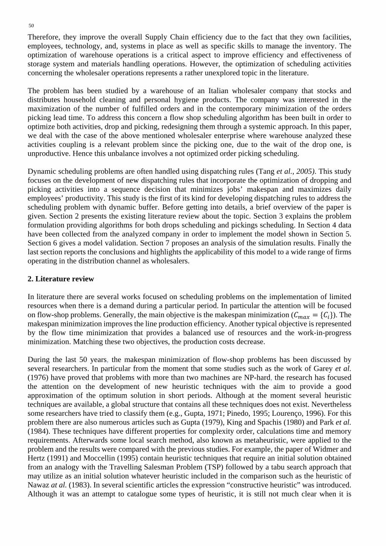
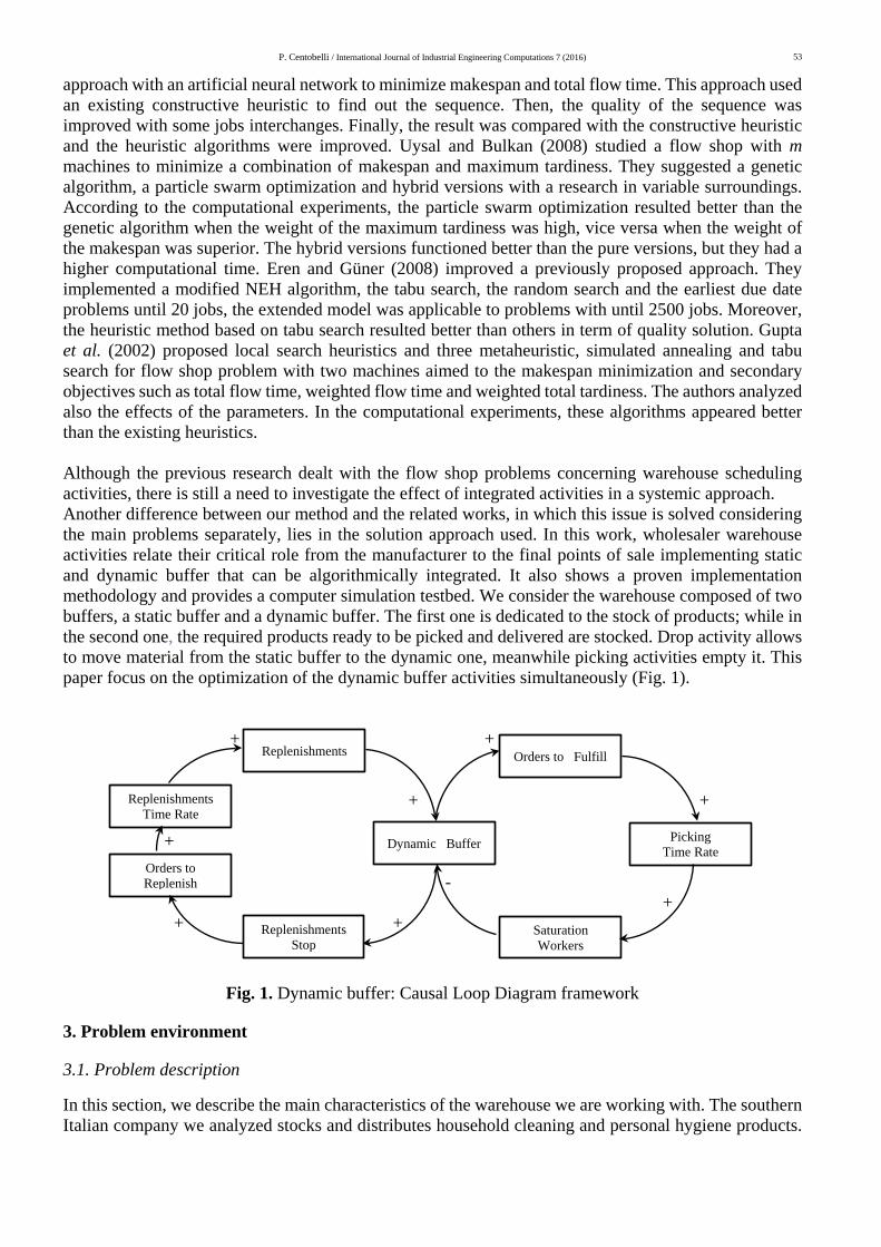
approach with an artificial neural network to minimize makespan and total flow time. This approach used an existing constructive heuristic to find out the sequence. Then, the quality of the sequence was improved with some jobs interchanges. Finally, the result was compared with the constructive heuristic and the heuristic algorithms were improved. Uysal and Bulkan (2008) studied a flow shop with m machines to minimize a combination of makespan and maximum tardiness. They suggested a genetic algorithm, a particle swarm optimization and hybrid versions with a research in variable surroundings. According to the computational experiments, the particle swarm optimization resulted better than the genetic algorithm when the weight of the maximum tardiness was high, vice versa when the weight of the makespan was superior. The hybrid versions functioned better than the pure versions, but they had a higher computational time. Eren and Güner (2008) improved a previously proposed approach. They implemented a modified NEH algorithm, the tabu search, the random search and the earliest due date problems until 20 jobs, the extended model was applicable to problems with until 2500 jobs. Moreover, the heuristic method based on tabu search resulted better than others in term of quality solution. Gupta et al. (2002) proposed local search heuristics and three metaheuristic, simulated annealing and tabu search for flow shop problem with two machines aimed to the makespan minimization and secondary objectives such as total flow time, weighted flow time and weighted total tardiness. The authors analyzed also the effects of the parameters. In the computational experiments, these algorithms appeared better than the existing heuristics. Although the previous research dealt with the flow shop problems concerning warehouse scheduling activities, there is still a need to investigate the effect of integrated activities in a systemic approach. Another difference between our method and the related works, in which this issue is solved considering the main problems separately, lies in the solution approach used. In this work, wholesaler warehouse activities relate their critical role from the manufacturer to the final points of sale implementing static and dynamic buffer that can be algorithmically integrated. It also shows a proven implementation methodology and provides a computer simulation testbed. We consider the warehouse composed of two buffers, a static buffer and a dynamic buffer. The first one is dedicated to the stock of products; while in the second one, the required products ready to be picked and delivered are stocked. Drop activity allows to move material from the static buffer to the dynamic one, meanwhile picking activities empty it. This paper focus on the optimization of the dynamic buffer activities simultaneously (Fig. 1).

+ + + +

+

- + + +

Fig. 1. Dynamic buffer: Causal Loop Diagram framework

3. Problem environment

3.1. Problem description

In this section, we describe the main characteristics of the warehouse we are working with. The southern Italian company we analyzed stocks and distributes household cleaning and personal hygiene products.

Replenishments

Replenishments Time Rate

Orders to Replenish

Replenishments Stop

Dynamic Buffer

Orders to Fulfill

Picking Time Rate

Saturation Workers

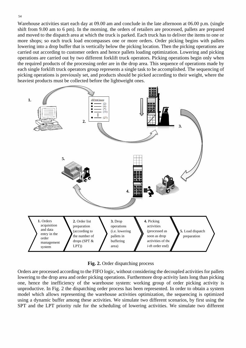
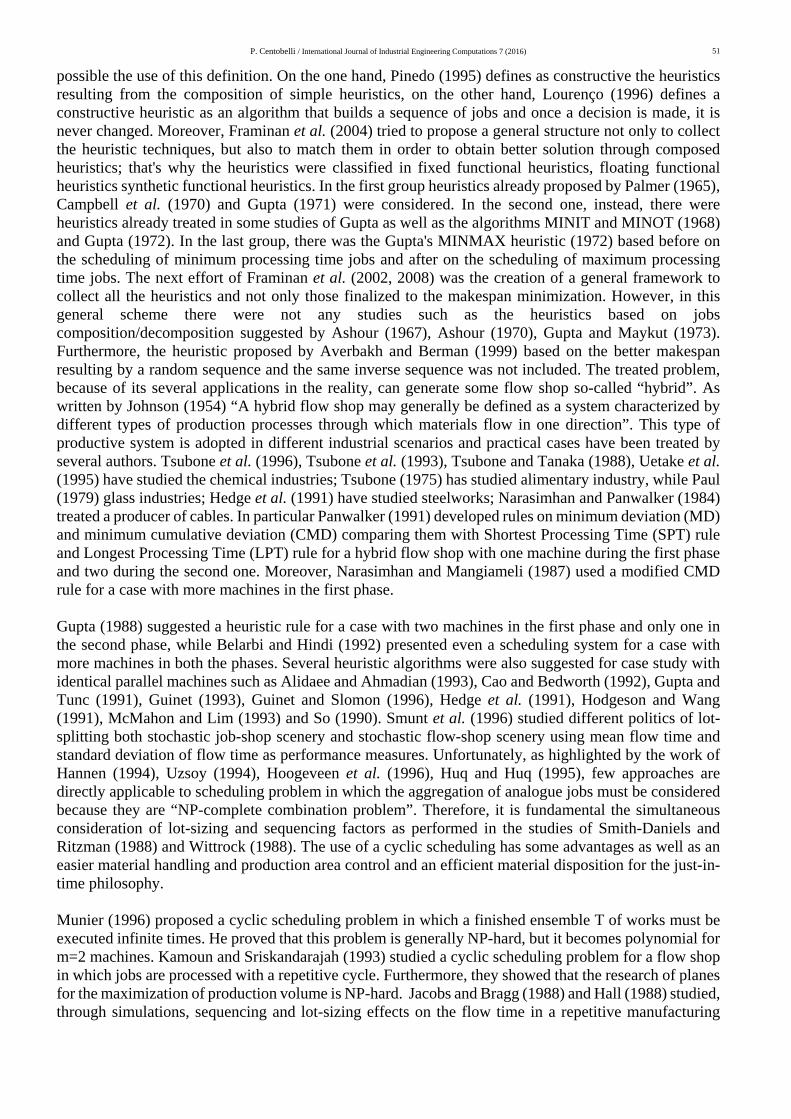
54 Warehouse activities start each day at 09.00 am and conclude in the late afternoon at 06.00 p.m. (single shift from 9.00 am to 6 pm). In the morning, the orders of retailers are processed, pallets are prepared and moved to the dispatch area at which the truck is parked. Each truck has to deliver the items to one or more shops; so each truck load encompasses one or more orders. Order picking begins with pallets lowering into a drop buffer that is vertically below the picking location. Then the picking operations are carried out according to customer orders and hence pallets loading optimization. Lowering and picking operations are carried out by two different forklift truck operators. Picking operations begin only when the required products of the processing order are in the drop area. This sequence of operations made by each single forklift truck operators group represents a single task to be accomplished. The sequencing of picking operations is previously set, and products should be picked according to their weight, where the heaviest products must be collected before the lightweight ones.

1. 2. 3. 5. 4.

Fig. 2. Order dispatching process

Orders are processed according to the FIFO logic, without considering the decoupled activities for pallets lowering to the drop area and order picking operations. Furthermore drop activity lasts long than picking one, hence the inefficiency of the warehouse system: working group of order picking activity is unproductive. In Fig. 2 the dispatching order process has been represented. In order to obtain a system model which allows representing the warehouse activities optimization, the sequencing is optimized using a dynamic buffer among these activities. We simulate two different scenarios, by first using the SPT and the LPT priority rule for the scheduling of lowering activities. We simulate two different

1. Orders acquisition and data entry in the order management system

2. Order list preparation (according to the number of drops (SPT & LPT))

3. Drop operations (i.e. lowering pallets in buffering area)

4. Picking activities (processed as soon as drop activities of the i-th order end)

5. Load dispatch preparation

P. Centobelli / International Journal of Industrial Engineering Computations 7 (2016)

55

scenarios, by using firstly the SPT and secondly the LPT priority rule for the scheduling of lowering activities. 3.2 Terminology and algorithm The mathematic formulation is specific for the sequencing in a flow shop problem implemented for warehousing activities in all those companies working in the Mass Retail Channel. This flow-shop presents a quite general structure consisting of two main activities: materials handling from a static buffer to a dynamic buffer and emptying of the dynamic buffer to deliver products. The two activities are generally identified as “drop” and “picking”. How this activities are executed influences performance parameters as well as delivery time and the number of daily dispatched orders.

In this article, drop and picking activities are combined to obtain the objective function for maximize the number of daily orders processed, i.e. minimize the difference between the overall working daily hours and the time required to fulfil orders. For the drop activities sequencing the following two cases are considered:

a. Shortest Processing Time (SPT), b. Longest Processing Time (LPT),

where Processing Time is the total number of drops necessary to allow to start picking activities in order to complete a customer order to be loaded. Before explaining the problem formulation, the notations used are presented: i index that identifies the orders within a load; it goes from 1 to n j index that identifies the different loads; it goes from 1 to m g index that identifies the product; it goes from 1 to s k index that identifies the iteration C(k) set of loads Cj waiting during the iteration k C’(k) set of loads Cj prepared during the iteration k C”(k) set of loads CjOij generated during the iteration k O (k) set of orders Oij waiting during the iteration k O’ (k) set of orders Oij for which the drop phase results completed and they are waiting the picking

phase O”(k) set of orders Oij prepared during the iteration k O”’(k) set of orders Oij generated during the iteration k Aij (k) Total num. of drops of the generic order i of the generic load j waiting during the iteration k A’ij (k) Total num. of drops of the generic order i of the generic load j carried out during the iteration

k A”ij (k) Total num. of drops of the generic order i of the generic load j generated during the iteration

k wg weight (expressed in kg) of the g-th product xg (k) stock, expressed in number of packages, of the g-th product in picking position during the

iteration k ẍgij (k) demand, expressed as number of packages, of the g-th product in the generic order i of the

generic load j agij (k) binary variables that identify the necessity (or not) to carry out a drop of products Pij (k) No. pickings of the generic order i of the generic load j waiting during the iteration k P’ij (k) No. pickings of the generic order i of the generic load j carried out during the iteration k P”ij (k) No. pickings of the generic order i of the generic load j generated during the iteration k tw total working time ta drop per unit time tp picking per unit time ts setup time

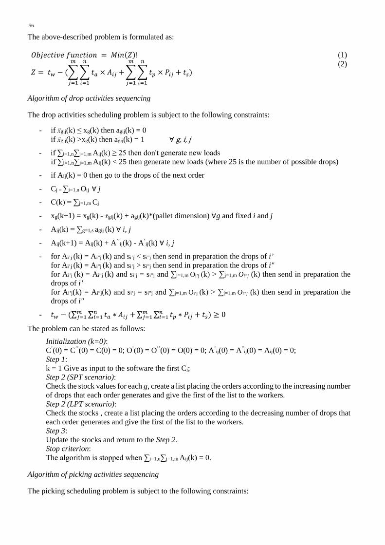
56 The above-described problem is formulated as:

𝑂𝑂𝑂𝑂𝑂𝑂𝑂𝑂𝑂𝑂𝑂𝑂𝑂𝑂𝑂𝑂𝑂𝑂 𝑓𝑓𝑓𝑓𝑓𝑓𝑂𝑂𝑂𝑂𝑂𝑂𝑓𝑓𝑓𝑓 = 𝑀𝑀𝑂𝑂𝑓𝑓(𝑍𝑍)! (1)

𝑍𝑍 = 𝑂𝑂𝑤𝑤 − (� � 𝑂𝑂𝑚𝑚 × 𝐴𝐴𝑖𝑖𝑖𝑖

𝑛𝑛

𝑖𝑖=1

+𝑚𝑚

𝑖𝑖=1

� � 𝑂𝑂𝑝𝑝 × 𝑃𝑃𝑖𝑖𝑖𝑖

𝑛𝑛

𝑖𝑖=1

+ 𝑂𝑂𝑠𝑠)𝑚𝑚

𝑖𝑖=1

(2)

Algorithm of drop activities sequencing

The drop activities scheduling problem is subject to the following constraints:

- if ẍgij(k) ≤ xg(k) then agij(k) = 0 if ẍgij(k) >xg(k) then agij(k) = 1 ∀ g, i, j

- if ∑i=1,n∑j=1,m Aij(k) ≥ 25 then don't generate new loads if ∑i=1,n∑j=1,m Aij(k) < 25 then generate new loads (where 25 is the number of possible drops)

- if Aij(k) = 0 then go to the drops of the next order

- Cj = ∑i=1,n Oij ∀ j

- C(k) = ∑j=1,m Cj

- xg(k+1) = xg(k) - ẍgij(k) + agij(k)*(pallet dimension) ∀g and fixed i and j

- Aij(k) = ∑g=1,s agij (k) ∀ i, j

- Aij(k+1) = Aij(k) + A’’ij(k) - A’ij(k) ∀ i, j

- for Ai’j (k) = Ai”j (k) and si’j < si”j then send in preparation the drops of i’ for Ai’j (k) = Ai”j (k) and si’j > si”j then send in preparation the drops of i" for Ai’j (k) = Ai”j (k) and si’j = si”j and ∑j=1,m Oi’j (k) > ∑j=1,m Oi”j (k) then send in preparation the drops of i’ for Ai’j(k) = Ai”j(k) and si’j = si”j and ∑j=1,m Oi’j (k) > ∑j=1,m Oi”j (k) then send in preparation the drops of i"

- 𝑂𝑂𝑤𝑤 − (∑ ∑ 𝑂𝑂𝑚𝑚 ∗ 𝐴𝐴𝑖𝑖𝑖𝑖𝑛𝑛𝑖𝑖=1 +𝑚𝑚

𝑖𝑖=1 ∑ ∑ 𝑂𝑂𝑝𝑝 ∗ 𝑃𝑃𝑖𝑖𝑖𝑖𝑛𝑛𝑖𝑖=1 + 𝑂𝑂𝑠𝑠)𝑚𝑚

𝑖𝑖=1 ≥ 0

The problem can be stated as follows:

Initialization (k=0): C’(0) = C’’(0) = C(0) = 0; O’(0) = O’’(0) = O(0) = 0; A’ij(0) = A”ij(0) = Aij(0) = 0; Step 1: k = 1 Give as input to the software the first Cj; Step 2 (SPT scenario): Check the stock values for each g, create a list placing the orders according to the increasing number of drops that each order generates and give the first of the list to the workers. Step 2 (LPT scenario): Check the stocks , create a list placing the orders according to the decreasing number of drops that each order generates and give the first of the list to the workers. Step 3: Update the stocks and return to the Step 2. Stop criterion: The algorithm is stopped when ∑i=1,n∑j=1,m Aij(k) = 0.

Algorithm of picking activities sequencing

The picking scheduling problem is subject to the following constraints:

P. Centobelli / International Journal of Industrial Engineering Computations 7 (2016)

57

- if Aij(k) = 0 then pick; - Cj = ∑i=1,n Oij∀ j = 1,…..,m; - C(k) = ∑j=1,m Cj; - Pij(k+1) = Pij(k) + P’’ij(k) - P’ij(k)∀i, j

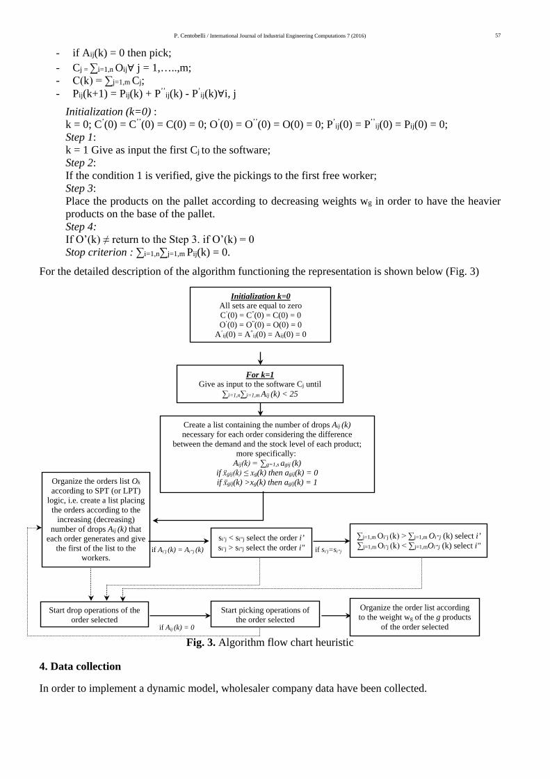
Initialization (k=0) : k = 0; C’(0) = C’’(0) = C(0) = 0; O’(0) = O’’(0) = O(0) = 0; P’ij(0) = P’’ij(0) = Pij(0) = 0; Step 1: k = 1 Give as input the first Cj to the software; Step 2: If the condition 1 is verified, give the pickings to the first free worker; Step 3: Place the products on the pallet according to decreasing weights wg in order to have the heavier products on the base of the pallet. Step 4: If O’(k) ≠ return to the Step 3. if O’(k) = 0 Stop criterion : ∑i=1,n∑j=1,m Pij(k) = 0.

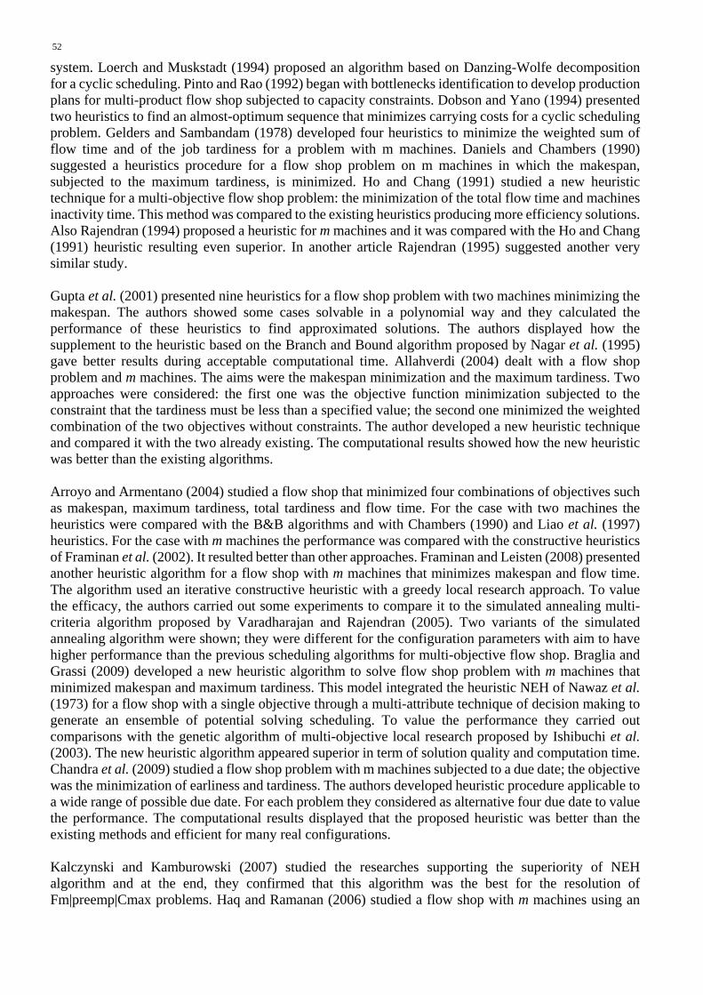
For the detailed description of the algorithm functioning the representation is shown below (Fig. 3)

Fig. 3. Algorithm flow chart heuristic

4. Data collection

In order to implement a dynamic model, wholesaler company data have been collected.

Initialization k=0 All sets are equal to zero

C(0) = 0(0) = ”(0) = C’C (0) = O(0) = 0”(0) = O’O

(0) = 0ij(0) = Aij”(0) = Aij’A

For k=1 until jGive as input to the software C

(k) < 25ij Aj=1,m ∑i=1,n∑

(k)ij ACreate a list containing the number of drops necessary for each order considering the difference

between the demand and the stock level of each product; more specifically:

(k)gij ag=1,s (k) = ∑ijA (k) = 0gij(k) then ag(k) ≤ xgijẍif (k) = 1gij(k) then ag(k) >xgijẍif

kOOrganize the orders list

according to SPT (or LPT) logic, i.e. create a list placing

the orders according to the increasing (decreasing)

that (k)ij Anumber of drops each order generates and give

the first of the list to the workers.

i’select the order i”j< s i’js i"select the order i”j> s i’js (k)i”j (k) = Ai’j Aif

i”j=si’jsif

i’(k) select i”jOj=1,m (k) > ∑i’j Oj=1,m ∑ i"(k) select i”jOj=1,m(k) < ∑i’j Oj=1,m ∑

Start drop operations of the order selected

(k) = 0ij Aif

Start picking operations of the order selected

Organize the order list according products gof the gto the weight w

of the order selected

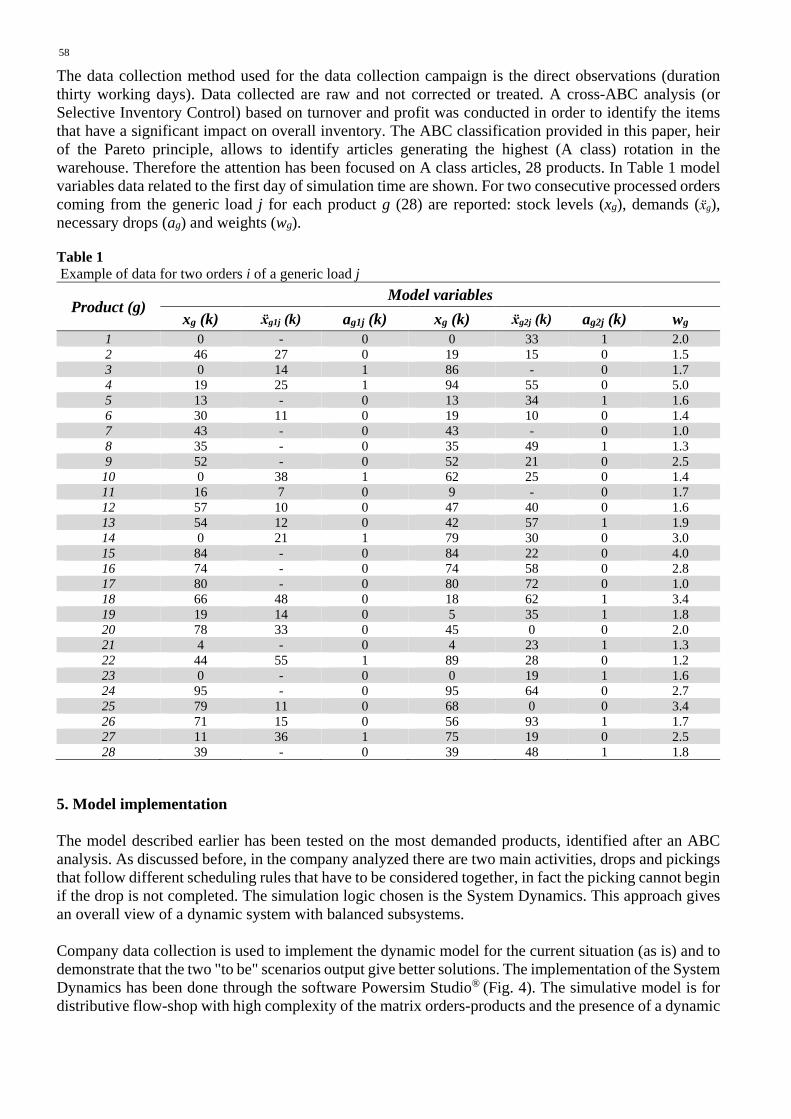
58 The data collection method used for the data collection campaign is the direct observations (duration thirty working days). Data collected are raw and not corrected or treated. A cross-ABC analysis (or Selective Inventory Control) based on turnover and profit was conducted in order to identify the items that have a significant impact on overall inventory. The ABC classification provided in this paper, heir of the Pareto principle, allows to identify articles generating the highest (A class) rotation in the warehouse. Therefore the attention has been focused on A class articles, 28 products. In Table 1 model variables data related to the first day of simulation time are shown. For two consecutive processed orders coming from the generic load j for each product g (28) are reported: stock levels (xg), demands (ẍg), necessary drops (ag) and weights (wg). Table 1 Example of data for two orders i of a generic load j

Product (g) Model variables

xg (k) ẍg1j (k) ag1j (k) xg (k) ẍg2j (k) ag2j (k) wg 1 0 - 0 0 33 1 2.0 2 46 27 0 19 15 0 1.5 3 0 14 1 86 - 0 1.7 4 19 25 1 94 55 0 5.0 5 13 - 0 13 34 1 1.6 6 30 11 0 19 10 0 1.4 7 43 - 0 43 - 0 1.0 8 35 - 0 35 49 1 1.3 9 52 - 0 52 21 0 2.5

10 0 38 1 62 25 0 1.4 11 16 7 0 9 - 0 1.7 12 57 10 0 47 40 0 1.6 13 54 12 0 42 57 1 1.9 14 0 21 1 79 30 0 3.0 15 84 - 0 84 22 0 4.0 16 74 - 0 74 58 0 2.8 17 80 - 0 80 72 0 1.0 18 66 48 0 18 62 1 3.4 19 19 14 0 5 35 1 1.8 20 78 33 0 45 0 0 2.0 21 4 - 0 4 23 1 1.3 22 44 55 1 89 28 0 1.2 23 0 - 0 0 19 1 1.6 24 95 - 0 95 64 0 2.7 25 79 11 0 68 0 0 3.4 26 71 15 0 56 93 1 1.7 27 11 36 1 75 19 0 2.5 28 39 - 0 39 48 1 1.8

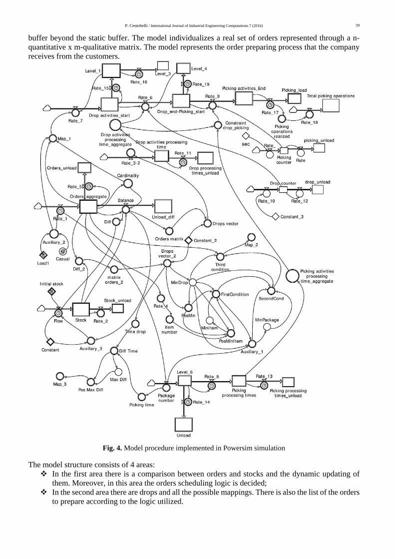
5. Model implementation The model described earlier has been tested on the most demanded products, identified after an ABC analysis. As discussed before, in the company analyzed there are two main activities, drops and pickings that follow different scheduling rules that have to be considered together, in fact the picking cannot begin if the drop is not completed. The simulation logic chosen is the System Dynamics. This approach gives an overall view of a dynamic system with balanced subsystems. Company data collection is used to implement the dynamic model for the current situation (as is) and to demonstrate that the two "to be" scenarios output give better solutions. The implementation of the System Dynamics has been done through the software Powersim Studio® (Fig. 4). The simulative model is for distributive flow-shop with high complexity of the matrix orders-products and the presence of a dynamic

P. Centobelli / International Journal of Industrial Engineering Computations 7 (2016)

59

buffer beyond the static buffer. The model individualizes a real set of orders represented through a n-quantitative x m-qualitative matrix. The model represents the order preparing process that the company receives from the customers.

Fig. 4. Model procedure implemented in Powersim simulation

The model structure consists of 4 areas: In the first area there is a comparison between orders and stocks and the dynamic updating of

them. Moreover, in this area the orders scheduling logic is decided; In the second area there are drops and all the possible mappings. There is also the list of the orders

to prepare according to the logic utilized.

60 The third area is the picking start. It contain only the orders for which the preparatory activities

are completed; The fourth area in which only the prepared orders can enter.

In particular, in the second area the model proposes three different mappings:

1. A logic based on a preloaded matrix ; 2. A logic based on the lower number of drops; 3. A logic based on the maximum difference between the picking times and the drop times.

The first mapping simulates whatever “as is” logic of a company belonging to the Mass Retailer Channel. The other two mappings are scenarios "to be" suggested to improve the number of daily satisfied orders. Data given as input to the system go from the 08/09/14 to the 17/10/14 and are in the rows "Actual Values". Instead, in the rows “Simulation Output” there are the results of the simulation according to the As Is scenario. Table 2 Actual values and simulation output (Prepared orders)

Day

1 2 3 4 5 6 7 8 9 10 11 12 13 14 15

ACTUAL VALUES 149 152 150 151 132 148 152 150 154 145 153 149 150 152 149

SIMULATION OUTPUT 152 154 152 153 135 150 154 152 157 147 155 151 152 154 152

Day

16 17 18 19 20 21 22 23 24 25 26 27 28 29 30

ACTUAL VALUES 153 139 154 149 150 154 145 148 152 154 149 151 153 151 150

SIMULATION OUTPUT 155 141 156 151 152 157 147 150 154 157 151 153 155 153 153

6. Model validation Although the actual values and the simulation outputs seem very similar, it is not enough to validate the model. For this reason a t-student test is necessary. This test compares the averages of two populations with unknown variance (but supposed equal), having the first order statistics (X̅1 e X̅2) and second order statistics (S12 e S22) of two big random sampling (n = m = 30). The following statistic is utilized:

𝒕𝒕 =𝒙𝒙�𝟏𝟏 − 𝒙𝒙�𝟐𝟐

𝑺𝑺�(𝟏𝟏/𝐧𝐧 + 𝟏𝟏/𝐦𝐦)

where S2represents the Pooled Variance :

𝑺𝑺𝟐𝟐 =(𝒏𝒏 − 𝟏𝟏)𝑺𝑺𝟏𝟏

𝟐𝟐 + (𝒎𝒎 − 𝟏𝟏)𝑺𝑺𝟐𝟐𝟐𝟐

𝒏𝒏 + 𝒎𝒎 − 𝟐𝟐

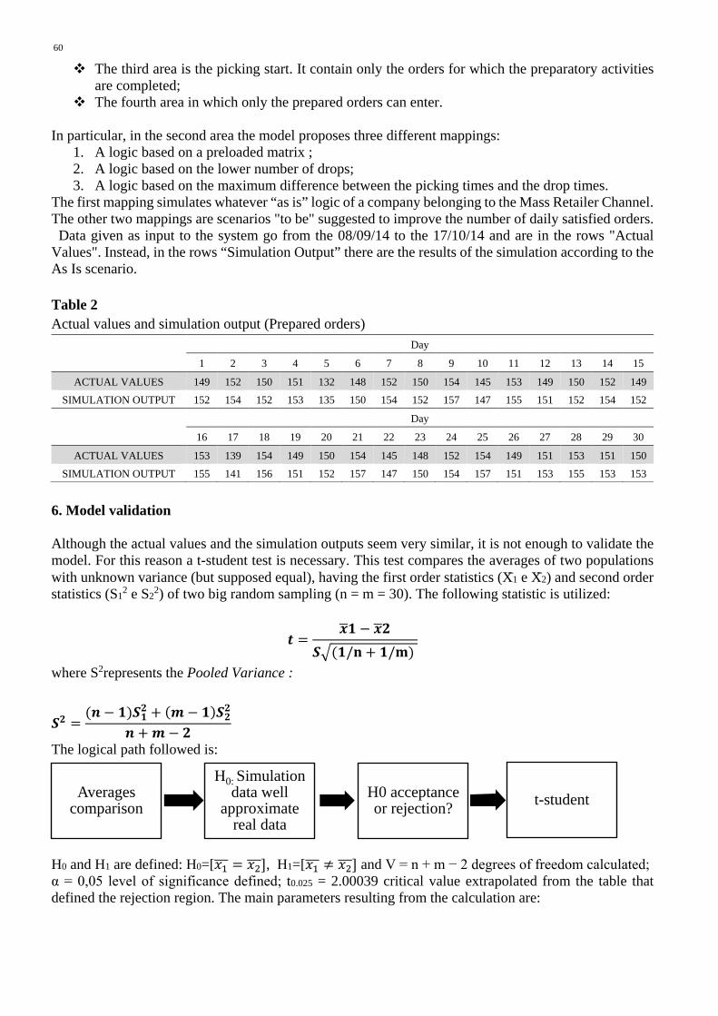
The logical path followed is:

H0 and H1 are defined: H0=[𝑥𝑥1��� = 𝑥𝑥2���], H1=[𝑥𝑥1��� ≠ 𝑥𝑥2���] and V = n + m − 2 degrees of freedom calculated; α = 0,05 level of significance defined; t0.025 = 2.00039 critical value extrapolated from the table that defined the rejection region. The main parameters resulting from the calculation are:

Averages comparison

H0: Simulation data well

approximate real data

H0 acceptance or rejection? t-student

P. Centobelli / International Journal of Industrial Engineering Computations 7 (2016)

61

�̅�𝑥1= 149.6; S12= 21.16; �̅�𝑥2= 151.8; S22= 20.97; S2 = 21.065; V = 58; t = 1.856

Because |t| < t0.025 the test is passed fixed a confidence level of 1-α=0.95.With the hypothesis testing a scientific validation of the model is given. 7. Analysis of the results Two parameters are compared between the 'as is' and the 'to be' scenarios.

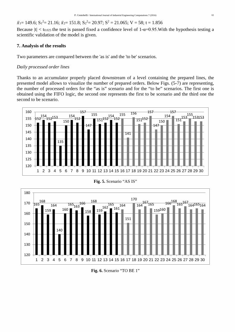
Daily processed order lines Thanks to an accumulator properly placed downstream of a level containing the prepared lines, the presented model allows to visualize the number of prepared orders. Below Figs. (5-7) are representing, the number of processed orders for the “as is” scenario and for the “to be” scenarios. The first one is obtained using the FIFO logic, the second one represents the first to be scenario and the third one the second to be scenario.

Fig. 5. Scenario “AS IS”

Fig. 6. Scenario “TO BE 1”

152154

152153

135

150154

152

157

147

155151152

154152

155

141

156

151152

157

147150

154157

151153

155153153

120

125

130

135

140

145

150

155

160

1 2 3 4 5 6 7 8 9 10 11 12 13 14 15 16 17 18 19 20 21 22 23 24 25 26 27 28 29 30

165168

159164

140

160165163

166

158

168

159162

165161

164

151

170164

167165159160

166168165167

164165164

120

130

140

150

160

170

180

1 2 3 4 5 6 7 8 9 10 11 12 13 14 15 16 17 18 19 20 21 22 23 24 25 26 27 28 29 30

62

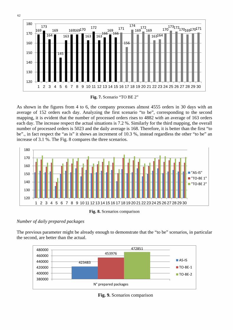
Fig. 7. Scenario “TO BE 2”

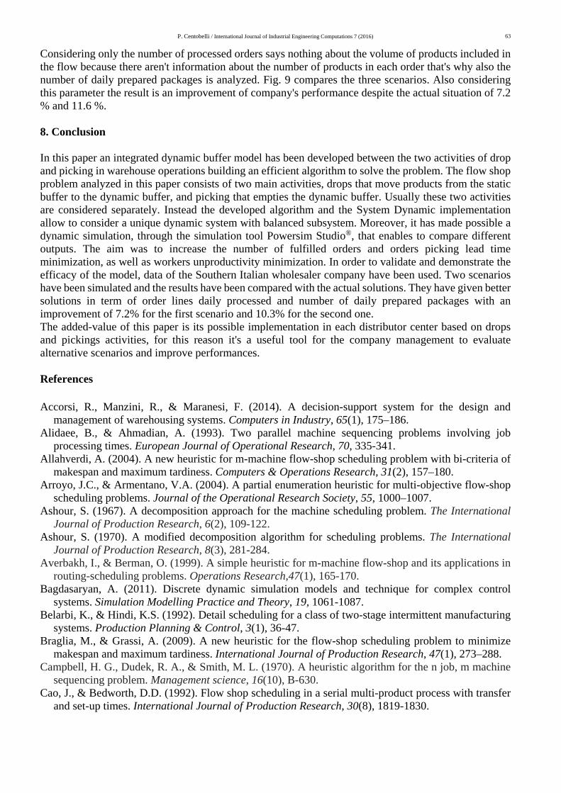
As shown in the figures from 4 to 6, the company processes almost 4555 orders in 30 days with an average of 152 orders each day. Analyzing the first scenario “to be”, corresponding to the second mapping, it is evident that the number of processed orders rises to 4882 with an average of 163 orders each day. The increase respect the actual situations is 7.2 %. Similarly for the third mapping, the overall number of processed orders is 5023 and the daily average is 168. Therefore, it is better than the first “to be”., in fact respect the “as is” it shows an increment of 10.3 %, instead regardless the other “to be” an increase of 3.1 %. The Fig. 8 compares the three scenarios.

Fig. 8. Scenarios comparison

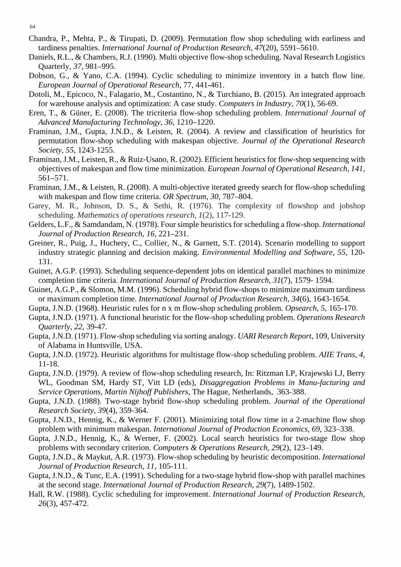
Number of daily prepared packages The previous parameter might be already enough to demonstrate that the “to be” scenarios, in particular the second, are better than the actual.

Fig. 9. Scenarios comparison

169173

164169

145

163169169170

163

172

163166

169166

171

156

174169

172169

163164170

173172170169170171

120

130

140

150

160

170

180

1 2 3 4 5 6 7 8 9 10 11 12 13 14 15 16 17 18 19 20 21 22 23 24 25 26 27 28 29 30

120

130

140

150

160

170

180

1 2 3 4 5 6 7 8 9 10 11 12 13 14 15 16 17 18 19 20 21 22 23 24 25 26 27 28 29 30

"AS-IS""TO-BE 1""TO-BE 2"

423483

453976472851

380000400000420000440000460000480000

N° prepared packages

AS-IS

TO-BE-1

TO-BE-2

P. Centobelli / International Journal of Industrial Engineering Computations 7 (2016)

63

Considering only the number of processed orders says nothing about the volume of products included in the flow because there aren't information about the number of products in each order that's why also the number of daily prepared packages is analyzed. Fig. 9 compares the three scenarios. Also considering this parameter the result is an improvement of company's performance despite the actual situation of 7.2 % and 11.6 %. 8. Conclusion In this paper an integrated dynamic buffer model has been developed between the two activities of drop and picking in warehouse operations building an efficient algorithm to solve the problem. The flow shop problem analyzed in this paper consists of two main activities, drops that move products from the static buffer to the dynamic buffer, and picking that empties the dynamic buffer. Usually these two activities are considered separately. Instead the developed algorithm and the System Dynamic implementation allow to consider a unique dynamic system with balanced subsystem. Moreover, it has made possible a dynamic simulation, through the simulation tool Powersim Studio®, that enables to compare different outputs. The aim was to increase the number of fulfilled orders and orders picking lead time minimization, as well as workers unproductivity minimization. In order to validate and demonstrate the efficacy of the model, data of the Southern Italian wholesaler company have been used. Two scenarios have been simulated and the results have been compared with the actual solutions. They have given better solutions in term of order lines daily processed and number of daily prepared packages with an improvement of 7.2% for the first scenario and 10.3% for the second one. The added-value of this paper is its possible implementation in each distributor center based on drops and pickings activities, for this reason it's a useful tool for the company management to evaluate alternative scenarios and improve performances. References Accorsi, R., Manzini, R., & Maranesi, F. (2014). A decision-support system for the design and

management of warehousing systems. Computers in Industry, 65(1), 175–186. Alidaee, B., & Ahmadian, A. (1993). Two parallel machine sequencing problems involving job

processing times. European Journal of Operational Research, 70, 335-341. Allahverdi, A. (2004). A new heuristic for m-machine flow-shop scheduling problem with bi-criteria of

makespan and maximum tardiness. Computers & Operations Research, 31(2), 157–180. Arroyo, J.C., & Armentano, V.A. (2004). A partial enumeration heuristic for multi-objective flow-shop

scheduling problems. Journal of the Operational Research Society, 55, 1000–1007. Ashour, S. (1967). A decomposition approach for the machine scheduling problem. The International

Journal of Production Research, 6(2), 109-122. Ashour, S. (1970). A modified decomposition algorithm for scheduling problems. The International

Journal of Production Research, 8(3), 281-284. Averbakh, I., & Berman, O. (1999). A simple heuristic for m-machine flow-shop and its applications in

routing-scheduling problems. Operations Research,47(1), 165-170. Bagdasaryan, A. (2011). Discrete dynamic simulation models and technique for complex control

systems. Simulation Modelling Practice and Theory, 19, 1061-1087. Belarbi, K., & Hindi, K.S. (1992). Detail scheduling for a class of two-stage intermittent manufacturing

systems. Production Planning & Control, 3(1), 36-47. Braglia, M., & Grassi, A. (2009). A new heuristic for the flow-shop scheduling problem to minimize

makespan and maximum tardiness. International Journal of Production Research, 47(1), 273–288. Campbell, H. G., Dudek, R. A., & Smith, M. L. (1970). A heuristic algorithm for the n job, m machine

sequencing problem. Management science, 16(10), B-630. Cao, J., & Bedworth, D.D. (1992). Flow shop scheduling in a serial multi-product process with transfer

and set-up times. International Journal of Production Research, 30(8), 1819-1830.

64 Chandra, P., Mehta, P., & Tirupati, D. (2009). Permutation flow shop scheduling with earliness and

tardiness penalties. International Journal of Production Research, 47(20), 5591–5610. Daniels, R.L., & Chambers, R.J. (1990). Multi objective flow-shop scheduling. Naval Research Logistics

Quarterly, 37, 981–995. Dobson, G., & Yano, C.A. (1994). Cyclic scheduling to minimize inventory in a batch flow line.

European Journal of Operational Research, 77, 441-461. Dotoli, M., Epicoco, N., Falagario, M., Costantino, N., & Turchiano, B. (2015). An integrated approach

for warehouse analysis and optimization: A case study. Computers in Industry, 70(1), 56-69. Eren, T., & Güner, E. (2008). The tricriteria flow-shop scheduling problem. International Journal of

Advanced Manufacturing Technology, 36, 1210–1220. Framinan, J.M., Gupta, J.N.D., & Leisten, R. (2004). A review and classification of heuristics for

permutation flow-shop scheduling with makespan objective. Journal of the Operational Research Society, 55, 1243-1255.

Framinan, J.M., Leisten, R., & Ruiz-Usano, R. (2002). Efficient heuristics for flow-shop sequencing with objectives of makespan and flow time minimization. European Journal of Operational Research, 141, 561–571.

Framinan, J.M., & Leisten, R. (2008). A multi-objective iterated greedy search for flow-shop scheduling with makespan and flow time criteria. OR Spectrum, 30, 787–804.

Garey, M. R., Johnson, D. S., & Sethi, R. (1976). The complexity of flowshop and jobshop scheduling. Mathematics of operations research, 1(2), 117-129.

Gelders, L.F., & Samdandam, N. (1978). Four simple heuristics for scheduling a flow-shop. International Journal of Production Research, 16, 221–231.

Greiner, R., Puig, J., Huchery, C., Collier, N., & Garnett, S.T. (2014). Scenario modelling to support industry strategic planning and decision making. Environmental Modelling and Software, 55, 120-131.

Guinet, A.G.P. (1993). Scheduling sequence-dependent jobs on identical parallel machines to minimize completion time criteria. International Journal of Production Research, 31(7), 1579- 1594.

Guinet, A.G.P., & Slomon, M.M. (1996). Scheduling hybrid flow-shops to minimize maximum tardiness or maximum completion time. International Journal of Production Research, 34(6), 1643-1654.

Gupta, J.N.D. (1968). Heuristic rules for n x m flow-shop scheduling problem. Opsearch, 5, 165-170. Gupta, J.N.D. (1971). A functional heuristic for the flow-shop scheduling problem. Operations Research

Quarterly, 22, 39-47. Gupta, J.N.D. (1971). Flow-shop scheduling via sorting analogy. UARI Research Report, 109, University

of Alabama in Huntsville, USA. Gupta, J.N.D. (1972). Heuristic algorithms for multistage flow-shop scheduling problem. AIIE Trans, 4,

11-18. Gupta, J.N.D. (1979). A review of flow-shop scheduling research, In: Ritzman LP, Krajewski LJ, Berry

WL, Goodman SM, Hardy ST, Vitt LD (eds), Disaggregation Problems in Manu-facturing and Service Operations, Martin Nijhoff Publishers, The Hague, Netherlands, 363-388.

Gupta, J.N.D. (1988). Two-stage hybrid flow-shop scheduling problem. Journal of the Operational Research Society, 39(4), 359-364.

Gupta, J.N.D., Hennig, K., & Werner F. (2001). Minimizing total flow time in a 2-machine flow shop problem with minimum makespan. International Journal of Production Economics, 69, 323–338.

Gupta, J.N.D., Hennig, K., & Werner, F. (2002). Local search heuristics for two-stage flow shop problems with secondary criterion. Computers & Operations Research, 29(2), 123–149.

Gupta, J.N.D., & Maykut, A.R. (1973). Flow-shop scheduling by heuristic decomposition. International Journal of Production Research, 11, 105-111.

Gupta, J.N.D., & Tunc, E.A. (1991). Scheduling for a two-stage hybrid flow-shop with parallel machines at the second stage. International Journal of Production Research, 29(7), 1489-1502.

Hall, R.W. (1988). Cyclic scheduling for improvement. International Journal of Production Research, 26(3), 457-472.

P. Centobelli / International Journal of Industrial Engineering Computations 7 (2016)

65

Hannen, C. (1994). Study of a NP-hard cyclic scheduling problem: The recurrent job-shop. European Journal of Production Research, 72, 82-101.

Haq, A., & Ramanan, TR. (2006). A bi-criterion flow shop scheduling using artificial neural network. International Journal of Advanced Manufacturing Technology, 3, 1132–1138.

Hedge, G.G., Shang, J.S., & Tadikamalla, P.R. (1991). An integrated approach for production planning - A case study. OMEGA, 19(5), 413-419.

Hedge, G.G., Shang, J.S., & Tadikamalla, P.R. (1991). An integrated approach for production planning-A case study, OMEGA, 19(5), 413-419.

Ho, J.C., & Chang, Y.L. (1991). A new heuristic for the n-job, m-machine flow-shop problem. European Journal of Operational Research, 52, 194–202.

Hodgeson, T.J., & Wang, D. (1991). Optimal hybrid push/pull control strategies for a parallel multistage system. International Journal of Production Research, 29(6), 1279-1287.

Hoogeveen, J.A., Lenstra, J.K., & Veltman, B. (1996). Primitive scheduling in a two-stage multiprocessor flow shop is NP-hard. European Journal of Operational Research, 89, 172-175.

Huq, F., & Huq, Z. (1995). The sensitivity of rule combination for scheduling in a hybrid job shop. International Journal of Operations & Production Management, 15(3), 59-75.

Ishibuchi, H., Yoshida, T., & Murata, T. (2003). Balance between genetic search and local search in memetic algorithms for multiobjective permutation flow-shop scheduling. IEEE Transactions on Evolutionary Computation, 7(2), 204–223.

Jacobs, F.R., & Bragg, D.J. (1988). Repetitive lots: Flow-time reductions through sequencing and dynamic batch sizing. Decision Sciences, 19, 281-294.

Johnson, S.M. (1954). Optimal two- and three-stage production schedules with setup times included. NavalResearch Logistics Quarterly, 1(l), 61-68.

Kalczynski, P.J.,& Kamburowski, J. (2007). On the NEH heuristic for minimizing the makespan in permutation flow shops. OMEGA–The International Journal of Management Science, 35(1), 53–60.

Kamoun, H., & Sriskandarajah, S. (1993). The complexity of scheduling jobs in repetitive manufacturing systems. European Journal of Production Research, 70, 350-364.

King, J.R., & Spachis, A.S. (1980). Heuristics for flow-shop scheduling. International Journal of Production Research, 18, 345-357.

Liao, C.-J., Yu, W.-C., & Joe, C.-B. (1997). Bicriterion scheduling in the two-machine flow- shop. Journal of the Operational Research Society, 48(9), 929–935.

Loerch, A.G., & Muckstadt, J.A. (1994). An approach to production planning and scheduling in cyclically scheduled manufacturing systems. International Journal of Production Research, 32(4), 851-871.

Lourenço, HR (1996). Sevast'yanov's algorithm for the flow-shop scheduling problem. European Journal of Operational Research, 91, 176-189.

McMahon, G.B., & Lim, C. (1993). The two-machine flow shop problem with arbitrary precedence relations. European Journal of Operational Research, 64, 249-257.

Moccellin, J.V. (1995). A new heuristic method for the permutation flow-shop scheduling problem. Journal of Operations Research Society, 46, 883-886.

Munier, A. (1996). The complexity of a cyclic scheduling problem with identical machines and precedence constraints. European Journal of Operational Research, 91, 471-480.

Nagar, A., Heragu, S.S., & Haddock J. (1995). A branch and bound approach for two- machine flow shop scheduling problem. Journal of the Operational Research Society, 46, 721–734.

Narasimhan, S. L., & Panwalker, S.S. (1984). Scheduling in a two-stage manufacturing process. International Journal of Production Research, 22(4), 555-564.

Narasimhan, S.L., & Mangiameli, P.M. (1987). A comparison of sequencing rules for a two-stage hybrid flow shop. Decision Sciences, 18, 250-265.

Nawaz, M., Enscore, E., & Ham I. (1983). A heuristic algorithm for the m-machine, n-job flow-shop sequencing problem. OMEGA–The International Journal of Management Science, 11(1), 91–95.

Nawaz, M., Enscore, E.E., & Ham, I. (1983). A heuristic algorithm for the m-machine, n-job flow-shop sequencing problem. Omega-International Journal of Management Science, 11, 91-95.

66 Palmer, D.S. (1965). Sequencing jobs through a multistage process in the minimum total time: a quick

method of obtaining a near-optimum. Operations Research Quarterly, 16, 101-107. Panwalker, S.S. (1991). Scheduling in a two-machine flow shop with travel time between machines.

Journal of the Operational Research Society, 42(7), 609-613. Park, Y.B., Pegden, C.D., & Enscore, E.E. (1984). A survey and evaluation of static flow-shop

scheduling heuristic. International Journal of Production Research, 22, 127-141. Paul, R.J. (1979). A production scheduling problem in the glass-container industry. Operations Research,

27, 290-302. Pinedo, M. (1995). Scheduling: Theory, Algorithms and Systems. Prentice-Hall: Englewood Cliffs, NJ. Pinto, P.A., & Rao, B.M. (1992). Joint lot-sizing and scheduling for multi-stage multi-product flow

shops. International Journal of Production Research, 30(5), 1137-1152. Rajendran, C. (1994). A heuristic algorithm for scheduling in flow-shop and flowline-based

manufacturing cell with multi-criteria. International Journal of Production Research, 32, 2541–2558. Rajendran, C. (1995). Heuristics for scheduling in flow-shop with multiple objectives. European Journal

of Operational Research, 82, 540–555. Smunt, T.L., Buss, D.H., & Kropp, D H. (1996). Lot splitting in stochastic flow shop and job shop

environments. Decision Sciences, 27, 215-238. So, K.C. (1990). Some heuristics for scheduling jobs on parallel machines with Setup. Management

Science, 36(4), 467-475. Tan, W., Chai, Y., Wang, W., & Liu, Y. (2012). General modeling and simulation for enterprise

operational decision-making problem: A policy-combination perspective. Simulation Modelling Practice and Theory, 21(1), 1-20.

Tang, L., Liu, W.,& Liu, J. (2005). A neural network model and algorithm for the hybrid flow shop scheduling problem in a dynamic environment. Journal of Intelligent Manufacturing, 16(3), 361-370.

Tsubone, H. (1975). Production scheduling system in the food manufacturing industry. 27th Conference Proceeding of Zennohren Society, Yamaguchi City, 240-244 (in Japanese).

Tsubone, H., Ohba, M., Takamuki, H., & Miyake, Y. (1993). A production scheduling system for a hybrid flow shop- A case study. OMEGA, 21(3), 205-214.

Tsubone, H., Ohba, M., & Uetake, T. (1996). The impact of lot sizing and sequencing on manufacturing performance in a two-stage hybrid flow shop. International Journal of Production Research, 34(l l), 3037-3054.

Tsubone, H., & Tanaka, T. (1988). Production scheduling system in the flow shop. OMEGA, 16(6), 608-611.

Uetake, T., Tsubone, H., & Ohba, M. (1995). A production scheduling system in a hybrid flow shop. International Journal of Production Economics, 41, 395- 398.

Uysal, O., & Bulkan, S. (2008). Comparison of genetic algorithm and particles warm optimization for bicriteria permutation flow-shop scheduling problem. International Journal of Computational Intelligence Research, 4(2), 159–175.

Uzsoy, U. (1994). Scheduling a single batch processing machine with non-identical job sizes. International Journal of Production Research, 32(7), 1615-1635.

Varadharajan, T.K., & Rajendran, C., (2005). A multi-objective simulated-annealing algorithm for scheduling in flow-shops to minimize the makespan and total flow time of jobs. European Journal of Operational Research, 167, 772–795.

Widmer, M., & Hertz, A. (1991). A new heuristic method for the flow-shop sequencing problem. European Journal of Operational Research, 41, 186-193.

Wittrock, R.J. (1988). An adaptable scheduling algorithm for flexible flow lines. Operations Research, 36(3), 445-453.