First and Second Generation Impacts of the Biafran War

Richard Akresh, Sonia Bhalotra, Marinella Leone, Una Osili∗

July 24, 2017

Abstract

We analyze long-term impacts of the 1967-1970 Nigerian Civil War, providing thefirst evidence of intergenerational impacts. Women exposed to the war in their grow-ing years exhibit reduced adult stature, increased likelihood of being overweight, earlierage at first birth, and lower educational attainment. Exposure to a primary educationprogram mitigates impacts of war exposure on education. War exposed men marrylater and have fewer children. War exposure of mothers (but not fathers) has adverseimpacts on child growth, survival, and education. Impacts vary with age of exposure.For mother and child health, the largest impacts stem from adolescent exposure.

JEL Codes: I12, I25, J13, O12Keywords: Intergenerational; Conflict; Human capital; Fetal origins; Africa

∗Akresh: University of Illinois at Urbana-Champaign, Email: akresh@illinois.edu; Bhalotra: Universityof Essex, Email: srbhal@essex.ac.uk; Leone: Institute of Development Studies, University of Sussex, Email:m.leone@ids.ac.uk; Osili: Indiana University-Purdue University Indianapolis, Email: uosili@iupui.edu; Wethank seminar participants at Bocconi University, University of Alicante, and at the CSAE, DIAL, HiCNand AEA conferences for helpful comments on earlier drafts.

1

1 Introduction

“Starvation is a legitimate weapon of war,and we have every intention of using it against the rebels.”

Mr. Alison Ayida, Head of Nigerian Delegation, Niamey Peace Talks, July 1968

More than fifty years ago, the Nigerian Civil War captured the world’s attention. The

war raged in Biafra, the secessionist region in the southeast of Nigeria from 6 July 1967 to

15 January 1970. It was the first modern civil war in sub-Saharan Africa after independence

and one of the bloodiest. About 1 to 3 million people died, mostly from starvation, sparking

a massive humanitarian crisis. The levels of starvation in Biafra were three times higher than

the starvation reported during World War II in Stalingrad and Holland (Alade, 1975; Mustell,

1977). War-induced food blockades led to severe protein shortages in the secessionist region

and caused widespread malnutrition and devastation among adults and children (Miller,

1970). The Biafra war ranks as one of the great nutritional disasters of modern times.

As it was one of the first post-World War II tragedies, Biafra drew the widespread atten-

tion of global religious and political leaders and gained extensive coverage in the international

media. It was the first African war to be televised, and millions around the globe witnessed

the large-scale devastation that ensued in the war-torn region. As one Western observer

noted: “This kind of tragedy was new to [television] viewers. Most hadn’t seen a starving

child in glorious Technicolor, looking like a matchstick, with a protruding stomach and the

reddish-brown hair that signals a slow death from starvation” (Waters, 2005, p.697). The

Biafran war triggered the rise of the international humanitarian movement, as several promi-

nent relief organizations, including Doctors without Borders, were formed to deal with the

war. However, relief efforts during the war were limited by the food blockades imposed by

the country’s military regime.

This paper contributes to an emerging literature on the legacies of war by producing

evidence of its long-term consequences. Since the Biafra war was waged half a century ago,

2

it presents an opportunity to analyze not only the long-run impacts but also impacts on the

next generation. This is relevant to understanding the formation of human capital and its

intergenerational transmission. While immediate adverse consequences of wars have been

well documented, long-run impacts have received far less attention. Studies of the longer run

economic effects of war have tended to conclude that economies are resilient, with capital

stocks having been rebuilt (Waldinger, 2011). However, the available evidence suggests that

human capital accumulation may be more permanently scarred following conflict, particu-

larly in developing countries.1 This is consistent with models of human capital formation in

which initial endowments and early investments have persistent and self-reinforcing impacts

on subsequent investments (Heckman and Schennach, 2008).

We examine impacts of the Biafran war on adult human capital (height, body mass

index (BMI), and education). We then present estimates for second generation outcomes,

including, child mortality (a marker of child health), anthropometrics, and education. We

attempt to provide a relatively comprehensive picture by linking first and second generation

impacts and presenting estimates for marriage, fertility, employment, and income for first

generation war-exposed women and men.2

Our identification strategy relies on evidence that ethnic groups indigenous to the seces-

sionist Biafra region (the Igbo being the most populous ethnic group) were the main victims

of the war, which was fought in Biafra. We interact ethnicity with the duration of expo-

sure to the war. We depart from many other studies documenting long-run consequences

of childhood shocks in adopting a flexible specification of exposure, allowing for age-specific

effects across a wide range of ages, from the fetal year through adolescence.

1Previous studies have documented long-run effects of exposure to stress (Camacho, 2008; Bozzoli andQuintana-Domeque, 2014; Quintana-Domeque and Rodenas-Serrano, 2014) and famine (Almond, 2006; Mac-cini and Yang, 2009), which are correlates of war exposure. Most existing research on war has focused on theeconomic and social burden during or shortly after the conflict (Akresh and De Walque, 2008; Bundervoetet al., 2009; Shemyakina, 2011; Mansour and Rees, 2012; Akresh et al., 2014; Valente, 2014). A handful ofrecent studies has started to explore long-term impacts of conflict on human capital accumulation (Migueland Roland, 2011; Akresh et al., 2012a,b; Leon, 2012; Justino et al., 2014; Akbulut-Yuksel, 2014, 2017) butno studies have documented evidence of intergenerational effects.

2All adult outcomes are, as in all related studies, conditional upon individuals having survived the war toadulthood. To the extent that survivors are positively selected, estimates of scarring are downward biased.

3

Our main findings are as follows. Women exposed to the war carry the scars of exposure

into adulthood, being shorter, more likely to be overweight, and less educated than unexposed

women. They start fertility at an earlier age, although we find no significant impacts on

their age at marriage or total fertility. We also find no significant impacts on employment

or wealth. Their children are more likely to die in early childhood and, if they survive,

exhibit growth stunting. There is also some evidence that they are less educated. We cannot

comprehensively identify the mechanisms generating the second generation impacts, but we

do find that war-exposed women are less likely to use prenatal care, skilled attendance at

birth, and safe delivery facilities.

The damaging effects of girls’ war exposure on their adult outcomes and on their chil-

dren’s outcomes are both increasing in age of exposure to the shock. Consistent with a

growing literature, we do find harmful effects of war exposure in utero and early childhood.

However, the adverse effects of war exposure are larger for women exposed during ages 13-

16.3 Adolescence is an age when a “second growth spurt” occurs (Case and Paxson, 2008b),

and this makes it plausible that nutritional deficits at this age have large effects; further

discussion of this is in section 3 where we also consider that the allocation of rationed food

to children of different ages may be a function of the distribution of work across children

of different ages. Our findings cohere with recently increasing attention directed towards

adolescence as a critical period in development (Leon, 2012; Aguero and Deolalikar, 2012;

Van den Berg et al., 2014, Caruso, forthcoming).

The effects are large, even though measured so long after the end of the war. Women

exposed to the war during adolescence for the average months of exposure (22.2 months) are

on average 4.53 centimeters shorter, 41 percentage points more likely to be overweight, and

11 percentage points less likely to complete secondary school. Their children suffer increases

of 1.5, 2.1, and 3.4 percentage points in neonatal, infant, and child mortality rates and if

they survive are 14 percentage points more likely to be stunted and 22 percentage points

3The age profile of the second generation results lines up with that in the first generation results.

4

more likely to be underweight. We investigate whether exposure to the Universal Primary

Education (UPE) Program initiated in 1976, six years after the end of the war, mitigated

impacts of the war on education. We find that it did - by almost 70 percent in states where

program resources were more intensively deployed.

We also examined long-run outcomes for war-exposed men. We do not have data on

men’s health, and we find no impact on their education, employment, or wealth. However

men exposed to the war marry later, have their first birth later, and have fewer children

overall. We find no deleterious impacts of father’s exposure on child survival or indicators

of child quality. This result is consistent with the condition of mothers being key in the

intergenerational transmission of human capital.

This paper links two strands of the literature. The first strand is on the long-run impact

of early life conditions on adult outcomes (Almond and Currie, 2011b,a) and critical periods

for investments in children (Cunha and Heckman, 2007). A few recent studies in economics

recognize that adolescence may be a critical period in height formation (Schultz, 2002; Case

and Paxson, 2008b) but there is limited (causal) evidence of the consequences of nutritional

deprivation at this age for other outcomes, and in particular, for next generation outcomes

(Benny et al., 2017). The second strand is on the intergenerational transmission of human

capital (Currie and Moretti, 2003, 2007; Almond et al., 2012; Bhalotra and Rawlings, 2013).

This paper makes the following contributions. First, it appears to be the first study

that identifies next-generation impacts of war, providing somewhat unique evidence of the

importance of maternal versus paternal war exposure, and some evidence of behavioral mech-

anisms. Second, it is one of the few papers to relax the common restriction that long-run

human capital is only malleable in early childhood. This is important as it suggests a po-

tential role for interventions in later childhood or that the scope for remediation is enlarged.

Third, in providing evidence that expansion of a free primary schooling initiative mitigated

the impacts of war exposure on education, it adds to still scarce evidence of how a positive in-

tervention following a negative shock can (partially) offset its impacts; this is relevant to the

5

double shocks literature (Almond and Mazumder, 2013; Adhvaryu et al., 2016; Rossin-Slater

and Wust, 2017) and also to a literature documenting pathways from health to educational

attainment (e.g., Almond and Currie, 2011a). Finally, it presents estimates not only for mea-

sures of human capital but also for marriage and fertility that are relevant to next-generation

impacts. However, we do not attempt to harness all results into a structural framework, and

the array of results we present merits further analysis and integration.

The rest of this paper is organized as follows. Section 2 provides background on the

Biafran war. Section 3 discusses the literature on early life shocks and the potential inter-

generational transmission of those shocks. Section 4 presents the data. Section 5 presents

the identification strategy. Section 6 presents results examining impacts of the war on a

range of first and second generation outcomes. Section 7 shows results analyzing the effects

of the mitigating effect of a free primary schooling program on first generation education

outcomes. Section 8 shows results of a number of robustness checks. Section 9 concludes.

2 Biafran War

Sub-Saharan Africa has experienced a disproportionate share of conflicts, with nearly three-

fourths of countries in this region having experienced armed conflict (Gleditsch et al., 2002).

Nigeria is an important country in which to study the long term consequences of war. Termed

the “Giant of Africa”, Nigeria is the most populous and one of the largest economies of sub-

Saharan Africa. The underlying causes of the Nigerian Civil War were complex (see Diamond,

1967; Sklar, 1967; Forsythe, 1969; Kirk-Greene, 1971; De St. Jorre, 1972; Nwankwo, 1972;

Madiebo, 1980; Jacobs, 1987; Stremlau, 2015). Nigeria gained independence from Great

Britain in 1960. Like many other African nations, at the time of independence Nigeria

was composed of diverse religious, economic, cultural, and ethno-linguistic groups that were

governed as semi-autonomous regions. Under colonial rule, Nigeria was a federation of three

regions: northern, western, and eastern, each populated mainly by three distinct ethnic

6

groups, Hausa, Yoruba, and Igbo respectively. The Northern region was predominantly

Muslim while the Eastern region was mainly Christian; both religions were present in the

Western region.

The fighting occurred principally in the Biafra region, located in southeastern Nigeria.

On May 30, 1967, Biafra declared itself an independent state. The Federal Government

declared this act of secession illegal. On July 6, 1967, which marked the onset of the war,

federal troops invaded the eastern region. The Northern armies of the ruling power advanced

into Biafra and pushed the Biafrans into a small enclave where food inflows were cut off.

The result was extensive famine among the Igbos and other minority Biafran ethnicities

(Miller, 1970). The Nigerian government did not initially allow international relief agencies

to reach the secessionist region. In August 1968, the first international relief operations were

launched but the amount of food proved insufficient to meet the demands of the affected

groups (Aall et al., 1970). The war ended on January 15, 1970 with the defeat of Biafra.

The secessionist region was characterized by a severe scarcity of proteins, as Biafra primarily

cultivated yams and cassava, and vast numbers of children developed kwashiorkor.

Recovery interventions in the Eastern States began after the war ended, enabled by an oil

boom that occurred in the 1970s, which provided an expansion in government resources. The

Nigerian government and international agencies attempted to reintegrate the war-affected

populations, repair the damage to physical infrastructure including health and educational

facilities, and restore social services and public utilities to war-affected regions (Ukpong,

1975). In 1976 the federal government introduced the Universal Primary Education program

(Osili and Long, 2008). As some of the war-exposed cohorts were also exposed to this

schooling expansion, we investigate the extent to which the UPE directly mitigated any war

impacts.

7

3 Mechanisms

A growing literature documents that investments made during critical periods of child de-

velopment draw larger returns or, conversely, that failure to invest can lead to irreversible

damage (Cunha and Heckman, 2007). As the Biafran War was a major nutritional shock

that occurred alongside reduced access to medical care and education, this paper is related to

studies that have analyzed sharp disruptions in the mother’s nutrition as a result of famine,

for example the Dutch Hunger Winter (Stein et al., 1975) and the Great Chinese Famine

(Almond et al., 2007; Chen and Zhou, 2007; Fung and Ha, 2010). However, these studies

restrict their analysis to in utero and early life exposure.

The focus on the fetal environment stems from biomedical research suggesting that

survival-motivated responses of the developing fetus to nutritional scarcity may get “coded”

in an irreversible manner, with potential elevation of later life health risks (Barker and Robin-

son, 1992; Gluckman and Hanson, 2004). Economists have documented influences of fetal

exposure on a range of socio-economic outcomes (Almond and Currie, 2011b). More recent

work establishes that there remains sufficient developmental plasticity in the year after birth,

with health shocks in infancy also being predictive of long-run socio-economic outcomes (Al-

mond et al., 2017; Bhalotra and Venkataramani, 2013, 2015) and life expectancy (Bhalotra

et al., forthcoming).

The reason that health and other investments in the early years matter is that physiologi-

cal and neurological development is especially rapid in these years. There are two reasons for

this. First, there is plasticity, the idea that shocks change the developmental path through

altering tissue structure and metabolic and endocrine processes. Second, early childhood is

a period of rapid growth and this makes young children particularly sensitive to nutritional

deprivation.

In fact, individuals experience a second growth spurt in adolescence (Case and Paxson,

2008b). Growth tends to remain rapid from birth until age three, then stabilizes until

adolescence at a rate of about 6 centimeters per year, after which it jumps to about 10

8

centimeters per year (Beard and Blaser, 2002).4 Yet there is surprisingly little research

investigating whether shocks in the adolescent years have any impacts that persist through to

adulthood. Although growth is rapid, there is less plasticity in some domains of development

and so the question of whether shocks that strike in the adolescent growth spurt leave

permanent scars is moot.

As detailed below, for the health and second generation outcomes, we find larger impacts

of war exposure in adolescence than in early childhood. Although both are intense periods of

growth, the increased nutritional demands may be greater for adolescents than for younger

children given their larger baseline size and this is moot given food shortages during the war.

Moreover, the intra-household allocation of food may reflect the intra-household allocation

of work. Although younger children often receive preferential treatment when resources are

scarce because their health is more sensitive to inputs, older children are more likely to

work and so may need more food (see Bhalotra and Attfield, 1998). In addition, individuals

who are stunted (nutritionally deprived) in infancy may experience catch-up growth as they

approach adolescence (Deaton, 2007; Benny et al., 2017) and so we may expect to see higher

nutritional demands in late childhood in resource-scarce environments than is generally the

case. An alternative interpretation of the identified age profile of scarring coefficients that

we shall attempt to investigate is that it reflects the age profile of selective mortality, with

mortality rates and hence selection decreasing in age.

Consider height and BMI, which are among the adult outcomes we analyze. Height is

widely used as a marker of the stock of health that correlates well with self-reported measures

of the stock of health and with life expectancy (Crimmins and Finch, 2006). A number of

previous studies show that adult height depends upon early childhood nutrition (Deaton,

2007; Bozzoli et al., 2009; Banerjee et al., 2010). However, there is limited evidence of

whether height responds to health shocks that occur in adolescence.5 BMI varies through

4Consistent with this age profile of the growth velocity, height-for-age Z-scores for girls in Ghana andCote d’Ivoire fall below a reference population of well-resourced children before the age of three and afterthe age of eleven but they track the reference population in the intervening age interval (Moradi, 2010).

5In a notable exception, in a paper emerging in parallel with our previous work on the Biafra war (Akresh

9

the life course and so is often used as a marker of short-term health, capturing contemporary

stresses (Dercon and Krishnan, 2000). However, recent research highlights that adult obesity

(BMI>30) may originate from fetal exposure to under-nutrition. Thus, it is more recently

recognized that BMI may also act as an indicator of the long-run persistent effects of early

life health. The biomedical literature suggests that if the under-nourished baby experiences

a diet high in fat and sugar later in life, then it is maladapted for this and hence at risk

of obesity, diabetes, and cardio-vascular disease (Barker and Robinson, 1992; Fung, 2010;

Gluckman and Hanson, 2006; Gluckman et al., 2011a,b). In fact there is evidence of this in

medical research on Biafra. Hult et al. (2010) use a sample of 40 year old Nigerian women

who were exposed to fetal and infant malnutrition during the Biafran war and document that

they had elevated rates of hypertension, diabetes, and obesity. However, we are unaware of

attempts to investigate whether health shocks in adolescence matter for BMI.

We also analyze impacts of war exposure on education, which may be influenced directly

through school closures or indirectly through impacts on health. We then look at downstream

outcomes that may depend on human capital, namely, marriage, fertility, employment, and

household wealth. The health indicators are only available for women, while the other

outcomes are available for men and women. The same exposure may have different impacts

on men and women for biological reasons and/or because of socially-conditioned differences

in responses to the shock (Akresh et al., 2011).

As regards mechanisms for impacts of war exposure of mothers on children, since we find

impacts of growing up in the war on multiple dimensions of the mother’s human capital and

we have just one instrument (war exposure), we cannot identify the pathways through which

the mother’s exposure impacts her children. However, previous work shows that mother’s

height and BMI are associated with risks of low birth weight and infant mortality in a

large sample of developing countries (Bhalotra and Rawlings, 2011), and there is evidence

that maternal obesity involves epigenetic processes that are transmitted to children (Dudley

et al., 2012a), Aguero and Deolalikar (2012) investigate impacts of the Rwandan genocide across the agedistribution and find an age profile similar to ours.

10

et al., 2011). Since we find no impacts of war exposure on income, it is unlikely that income

is a pathway. Women’s education may matter for example because it influences health

seeking behaviors (Currie and Moretti, 2003). We investigate such behavioral mechanisms

by modelling investments in early childhood inputs, prenatal care, and safe delivery as a

function of war exposure.

4 Data

The analysis uses the Nigeria Demographic Health Surveys (DHS) of 1999, 2003, and 2008.

These are large nationally representative cross-sectional surveys designed to provide demo-

graphic and health-related information. They contain data on women aged 15 to 49 at the

time of the survey. We observe them respectively 29, 33, and 38 years after the war ended

in 1970. The surveys also contain data on men aged 15 to 59 at the time of the survey.6

We restrict the sample to women born between 1954 and 1974. Those born before October

1970 were potentially exposed to the war from the fetal year to adolescence (depending on

their ethnicity), and the control cohorts are those born between November 1970 and 1974.

The second generation child-level sample includes all children of the mothers in the first

generation analysis (i.e., mothers born between 1954 and 1974). We restrict the analysis to

children born after 1970 to avoid the possibility that the children are directly exposed to the

war.7 For anthropometric outcomes, information is only available for children born in the

five years before the 2003 and 2008 surveys and the three years before the 1999 survey, so

for those analyses, the sample includes only children born between 1996 and 2008, again, to

mothers born between 1954 and 1974.8

For women, but not men, the data contain height and weight as indicators of health

6The Data Appendix provides more details about the surveys, the sample, and the variables analyzed.7Only 0.2 percent of children in the sample were born before 1970.8By definition, our sample only includes adult individuals who survived the war. This will tend to lead

us to under-estimate the war’s impact (Chay et al., 2009; Bozzoli et al., 2009). We provide a discussion ofpotential age-specific selective mortality in the robustness checks section, in relation to a discussion of theage-profile of war impacts.

11

measured by trained surveyors. We have information on schooling, fertility, marriage, em-

ployment, and wealth outcomes for both women and men.9

The DHS contain fertility histories, which allow us to extend the analysis to second

generation outcomes. The histories provide the gender and dates of birth and death (if

relevant) of all children. For surviving children up to age 18 at the time of the survey we

have information on their education, and for children who were born in the three to five

years preceding each survey date, we have anthropometric data.

We explore child mortality for the second-generation, which reflects the health environ-

ment at birth and in the early years of life as well as maternal health conditions (Bozzoli

et al., 2009; Bhalotra and Rawlings, 2013). We are able to measure neonatal, infant, and

under-five child mortality. We also analyze impacts of maternal war exposure on child nu-

tritional status. The height-for-age Z-score is an indicator of linear growth retardation and

cumulative growth deficits and it reflects the effects of persistent malnutrition (NPC, 2009,

p.164). Children whose height-for-age Z-score is below minus two standard deviations are

considered stunted and chronically malnourished. We examine child weight-for-age Z-scores,

which reflect short-term malnutrition. Children whose weight-for-age is below minus two

standard deviations are defined as underweight.

To investigate impacts on the second generation’s educational attainment, we can only

include information from the 2003 and 2008 DHS surveys as information on children’s edu-

cation is not included in the DHS 1999 survey.10 The sample is restricted to children aged

6 to 18 years old at the time of the survey to account for a school starting age of 6 and any

9The employment variable measures whether an individual worked in the past 12 months. Althoughthis is a more short-term indicator of labor supply, existing research using the same indicator shows that itcompares well across countries and years with the World Development Indicators aggregate data (Bhalotraand Umana-Aponte, 2010). The wealth index is constructed as part of the DHS survey data and is basedon data about the household’s ownership of consumer goods, dwelling characteristics, type of drinking watersources, toilet facilities, and other characteristics related to the household’s socio-economic status. Thisindex has been extensively used and exhibits the expected correlation with many variables (Filmer andPritchett, 2001).

10We transform years of education into a Z-score to account for the fact that some children may still be inschool. We calculate the deviation of a child’s completed years of schooling from the mean years of schoolingfor their age, gender, and survey round and divide this by the standard deviation in that three-way cell.

12

potential selectivity of children remaining at home.

Table 1 reports the summary statistics of the main variables of interest for the sample

analyzed. Adult women are on average 159 centimeters tall with a BMI of 24. Ten percent

of women are underweight while 31 percent are overweight. In the sample of first generation

women, the average years of schooling is 4.5, more than 50 percent have completed at least

primary school, and 27 percent have completed at least secondary school. On average, women

get married before age 18 and have over 5 children. The children of these women (second

generation) suffer extremely high child mortality with 18 percent dying before 60 months,

38 percent being stunted, and 28 percent being underweight.

5 Identification Strategy

Our identification strategy exploits the timing of the war jointly with the fact that the war

was entirely fought in the southeastern region of Nigeria (Biafra) where the Igbo and other

minority ethnic groups originated. We use a difference-in-differences specification, defining

an individual’s duration of exposure to the war (in months) at a given age as a function of

her ethnicity and birth cohort. An important distinguishing feature of the specification is

that it allows impacts of war exposure durations to vary by age at exposure.

5.1 First generation impacts

For the first generation analysis, we estimate the following equation:

Yimcesr = βamonths war exposuremc ∗ war ethnicitye (1)

+ δamonths war exposuremc + αc + θe + λs + µr + γe.t+ uimcesr

The subscripts i, m, c, e, s, and r index an individual i, born in month m and year c,

of ethnicity e, resident in state s, whose outcome, Y , is measured in survey round r. The

13

outcomes are indicators of health, education, marriage, fertility, employment, and income.

The independent variable of interest, months of war exposure*war ethnicity is constructed

as a vector with age-specific coefficients. The equation includes the main effect of months

of war exposure, allowing for the war to influence the control group, and it includes fixed

effects for birth year, αc. Although there is a strong overlap of ethnicity and state, they

are not identical, so we include both ethnicity and state fixed effects, θe and λs. We control

for ethnicity-specific time trends to allow for any underlying divergence or convergence in

outcomes across ethnic groups over time. We also include survey round fixed effects, µr, and

u is a random, idiosyncratic error term.11 The coefficients βa and δa vary with the age at

which the individual was exposed to the war. The coefficients βa indicate the causal impact

of war exposure under the standard identifying assumptions in a difference-in-differences

model. The coefficients δa capture any potential spillovers and tell us whether the non-war

ethnicity groups suffered from the war. The full impact of the war on war-exposed ethnicities

for a given age cohort is βa + δa.

We define war ethnicity as being Igbo or another minority ethnic group (Adoni, Adun,

Annang, Efik, Ekoi, and Ibibio) from the Biafran region. Most previous research studying

the impact of war uses geographical variation in conflict intensity, but that approach can

be sensitive to selective migration. By using ethnic variation to measure war exposure, we

minimize this problem as people maintain their ethnicity if they migrate. In robustness

checks discussed in Section 8, results are similar when we use regional variation to measure

war exposure.

We use information on the month and year of birth of each individual to construct the

duration of war exposure in months, which ranges from 0 months if they were never exposed

to 31 months if they lived through the entire war. All individuals in the sample born between

1954 (the earliest birth cohort in the sample) and October 1970 are war-exposed. The war

11To allow for correlation among the error terms within ethnic group and birth cohort, we cluster allstandard errors at the ethnicity and birth year level (Moulton, 1986). The statistical significance of theresults is similar if we instead cluster the standard errors at the ethnicity level.

14

ended in January 1970, but individuals born before October 1970 would have experienced

in utero exposure to the war. Non-exposed individuals consist of post-war births from

November 1970 (ten months after the end of the war to avoid in utero war exposure) until

December 1974. We select a narrow window for the control group since the potential for

confounding events increases with window size.12

Our differentiation of war exposure by age allows for the possibility that being exposed

to the war for any given duration may be more harmful at a critical age than at another age.

To reduce measurement error in age and gain precision, we group ages into five categories,

in utero, ages 0-3, 4-6, 7-12, and 13-16. Age banding also allows for slight variation in the

timing of the early childhood and puberty growth spurts that even in non-war conditions

will arise from differences in baseline socioeconomic status across girls (Case and Paxson,

2008a). The age bands are constructed with reference to the relationship between age and

height growth (Case and Paxson, 2008b) and map reasonably well into preschool and school

age thresholds.

Since we have three to four measures of each of the health and education outcomes, we

adjusted for multiple hypothesis testing following the Hochberg step-up method (Hochberg,

1988). We also investigated replacing ethnicity, which is time invariant, with an ethnicity-

specific time-varying measure that captures variation in war intensity over time (labeled

ethnic mortality in the tables). We create this variable using information from the 2008

DHS survey that asked women to report the dates of birth and death of each of their

siblings. We define ethnic mortality as the percentage change at the ethnicity level in sibling

mortality rates between the war years (1967-1970) and the post-war years (1973-1976).13

The constructed ethnic mortality variable is interacted with months of war exposure in the

12We explore sensitivity of our results to this decision about the appropriate control group cohort window,and our findings in general hold with a longer post-war cohort window.

13More precisely, the mortality rate during the war years is calculated as the ratio of the number of siblingswho died during the war and the total number of siblings born up to 1970. Similarly, the post-war mortalityrate is calculated as the ratio of the number of siblings who died after the war (between 1973 and 1976) andthe number of siblings born up to 1976. The Data Appendix presents in more detail the construction of thisindicator.

15

same way that ethnicity is in the baseline specification.

5.2 Second generation impacts

Sufficient time has elapsed since the Biafra war that we are able to analyze whether it has

cast a shadow so long as to impact the children of individuals who were exposed to the

war in their childhood. To measure second generation impacts, we estimate the following

regression:

Yotimcesr = βamother’s months war exposuremc ∗ war ethnicitye (2)

+ δamother’s months war exposuremc + αt + αc + θe

+ λs + µr + γe.t+ uotimcesr

The subscripts o, t, i, m, c, e, s, and r index a child o, born in year t, to a woman i, who

was born in month m and year c, of ethnicity e, and resident in state s. The child’s outcome,

Y , is measured in round r. The main variables of interest, mother’s months of war exposure

* war ethnicity are specified as in Equation 1. The equation also includes the main effect of

mother’s months of war exposure, as well as fixed effects for the child’s birth year, αt, and

the mother’s birth year, αc. We include a binary variable indicating if the child is female.

All other terms on the right hand side have the same meaning as in Equation 1 and refer

to the child’s mother. Similarly to the first generation analysis, we also investigated the

effects replacing ethnicity with ethnic mortality (as defined above). We also estimate similar

equations describing child outcomes as a function of the father’s exposure to the war.

6 Results

We present the first-generation results for women and men, followed by the second-generation

results. We find that the profile of coefficients by age of exposure of the mother for the

16

outcomes of her children is similar to that for her adult outcomes. This supports our in-

terpretation of the second-generation coefficients as arising via impacts due to the mother’s

war exposure. All tables contain two panels, one for each of the measures of war exposure.

In the upper panel, we interact duration of exposure with an indicator for the exposed eth-

nicity while, in the lower panel, we interact duration of exposure with a measure of excess

mortality of the exposed ethnicity during the war years. Group-level exposure in the first

panel is effectively replaced with an index of the intensity of exposure in the second panel.

6.1 First generation analysis

6.1.1 Health

Table 2 presents estimates for women of the baseline specification (Equation 1) for height,

BMI, underweight status, and overweight status. These health indicators are not available

for men. The overall picture is of a systematic tendency for war exposure to reduce adult

stature and increase BMI. Both are consistent with the war constituting a nutritional shock

in the growing years. The effects are large. We interpret this as a compelling statement of

the ruthlessness of this war.

Critical Ages. A striking finding is that there are significant effects of war exposure

right from birth (in the case of height) or the fetal period (in the case of BMI and obesity)

through to age 16. For all outcomes, the effects are increasing in age of exposure. Our

expectation was that the coefficient profile would be U-shaped, with large effects at the start

of life and in the teenage years, which are both growth spurts. Although growth is most

rapid soon after birth (ages 0-3), an adolescent growth spurt starts around the age of 12 or

13 for girls (Case and Paxson, 2008a) and a few other studies find, as we do, that shocks at

this age matter, (Aguero and Deolalikar, 2012; Van den Berg et al., 2014). So this explains

why adolescence matters. In section 3, we discussed potential explanations of why scarring

from exposure in adolescence may be greater than scarring from exposure in infancy.

Height. Girls who were exposed to the war between the ages of 0-3 for the average

17

duration of exposure experienced by this cohort (17.5 months) suffered a reduction in adult

height of 0.75 centimeters relative to unexposed girls of the same cohort.14 A similar calcu-

lation for girls exposed to the war between the ages of 13-16 for the average duration (20.6

months) suggests a 4.53 centimeter deficit in adult height. The results are similar using

estimated excess mortality among war exposed ethnicities during the war (Panel B).15

BMI. Results in Panel A show that women exposed to the war in childhood (in utero

through adolescence) exhibit a higher BMI and are more likely to be overweight (BMI above

25) as adults. There is no effect of war exposure on being underweight (BMI below 18.5).

These effects are larger for women exposed in adolescence, consistent with the results on

height. Girls exposed to the war between ages 13-16 for the average duration have a BMI

that is 4.5 points higher than non-war exposed girls, and the likelihood of being overweight

is 41 percentage points higher for these women. Results in Panel B are similar.

As discussed in Section 3, the literature on fetal origins provides evidence that children

exposed to nutritional shocks in early life may have smaller stature as adults and that the

changes in early life metabolism generated by nutritional scarcity create the potential for

maladaptation, leading to obesity in later life (Barker, 1998; Fung, 2010; Gluckman et al.,

2009). However, in contrast to that literature we document impacts on height and obesity

due to exposure beyond early childhood. In view of evidence that teenagers experience a

second growth spurt, it may be that scarcity in this later growing period also has persistent

effects. While the biomedical mechanisms for this are not well documented, there is related

14All effects sizes presented here are calculated multiplying the average duration of exposure to war experi-enced by each cohort that belongs to the war ethnicity by its related βa coefficient. Therefore, this measuresthe additional impact of war exposure for the war ethnicities.

15A common concern with difference-in-differences identification strategies is that there could be pre-trendsin the outcomes by (exposed versus unexposed) ethnicity. The inclusion of ethnicity and state fixed effectsand ethnicity specific time trends addresses the first-order concern. To assess this further, we also conductedthe following placebo test. We estimate regressions using alternative placebo war dates (December 1983 toJune 1986) assuming the war happened at a different time, which allows the same war duration (31 months)but 16 years later. We define the sample to include individuals born between November 1970 and 1990 sothat there is no overlap in exposure with the real war. Table A.1 shows results for the first generation healthoutcomes. All coefficients in the height placebo regressions are close to zero and statistically insignificant.Some coefficients on BMI (column 2 and 4) are statistically significant, but negative, which is the oppositeof the sign obtained when we use the actual war years.

18

evidence in a few other studies (Leon, 2012; Aguero and Deolalikar, 2012; Van den Berg

et al., 2014, Caruso, forthcoming).

6.1.2 Education

Table 3 shows estimates of the impact of war exposure on educational outcomes for women

and men. Overall, the evidence indicates some adverse impacts of war exposure on women’s

education (columns 1 to 3), although these are less robust than the results for height and

BMI. We see no evidence that the education of exposed men suffered (columns 4 to 6).

In the sample of women, there are consistently significant results in Panel B, where we

use the richer variation in ethnic differences in war mortality, rather than just ethnicity. We

find that educational attainment and the probability of completing primary school are lower

for women who were war exposed during early childhood (ages 0-3) or during the primary

school ages of 7-12. We also find lower rates of completion of secondary school among women

exposed to war during ages 0-16.16

Using the Panel B coefficients to assess magnitudes, we estimate that women exposed to

the war at ages 0-3 for the average months of war exposure (10.9 months) show 0.37 less years

of completed education and are 3 and 5 percentage points less likely to complete primary and

secondary school than non-exposed women.17 Women exposed at ages 7-12 (when average

exposure duration is 14.2 months) show larger deficits - a reduction in years of education of

0.92 years and a reduction in the probability of completing primary and secondary education

of 8 and 11 percentage points, respectively.18

16Our finding that war exposure at age 13-16 has no impact on years of education possibly reflects the factthat fewer children in these cohorts complete secondary school (only 12 percent of women and 31 percent ofmen in these cohorts complete secondary education.)

17In order to calculate the effect sizes in Panel B, we calculate the average difference between war exposedand non-war exposed ethnicities for mortality in war time versus peace time (i.e. the ethnic mortalityterm). We then multiply this difference (0.12) by the average months of war exposure and by the estimatedcoefficient. Doing this calculation delivers estimates that are very close to the coefficients in Panel A.

18We are not able to conduct a similar placebo falsification test for education as we did for health becausethe cohorts assigned to the placebo groups could have been affected by the UPE program. Instead, we exploitthe 1990 and 1999 DHS surveys, which contain information on the education outcomes of individuals bornbefore 1950, to estimate an alternative placebo test. We define the sample to include women born between1940 and 1950, with those women born 1945-1950 acting as the placebo war-exposed cohorts. Cohorts born

19

Our finding that women’s education suffered while men’s did not is consistent with lower

weight being placed on girls’ education. Recent research argues that factors that can tilt

the gendered impacts one way or the other include the specifics of the conflict, pre-war

differences in education levels by gender, and labor market and educational opportunities in

the absence of war (Buvinic et al., 2014; Akresh, 2016).19

Policy Remediation. Between 1976 and 1981, starting six years after the end of the

war, Nigeria launched a nation-wide expansion in primary schooling known as the Univer-

sal Primary Education program. The program gave all children six years of free primary

education, facilitated by increased funding for school construction, hiring new teachers, and

additional teacher training. This positive shock to education could have potentially miti-

gated some of the negative impacts of war exposure. Given the timing of when the UPE

program began and when the war ended, only the youngest cohorts in the Table 3 regres-

sions (in utero, ages 0-3, and ages 4-6) would have been of primary school age when the

UPE began. These cohorts would have been 6-15 years old in 1976 at the start of the UPE

program. It is possible that for these young cohorts who were subsequently exposed to the

UPE program we under-estimate the impacts of war exposure on education, which as we

discussed above were negative and meaningfully large. In contrast, the older cohorts (those

ages 7-16 during the war) would have been 13-25 when the UPE program started in 1976 and

hence would not have benefited from the UPE. In Section 7, we more formally examine the

confluence of these two natural experiments (war exposure and UPE exposure) to analyze

after 1950 could have been exposed to the war at age 16 or younger and so are excluded from this placeboanalysis. We regress education outcomes on the interaction between an indicator for women born from1945-1950 and an indicator for women residing in the war region. Ethnicity information is not availablein the DHS 1990 survey so we use regional variation to run this placebo test. We control for state fixedeffects, year of birth fixed effects, and state time trends. The results in table A.2 show that the coefficientson the difference-in-differences terms are not significant in any specifications, which suggest that trends ineducation outcomes before the war were similar between war and non-war regions.

19To highlight these factors, a study of the Nepal civil conflict from 1996 to 2006 illustrates just how muchdifference the context can make when it comes to a conflict’s effect on education (Valente, 2014). In districtsthat saw more casualties from the conflict, girls’ educational attainment increased. But in districts thatsaw more abductions by the Maoist insurgents, who often targeted school children, the opposite was true.Similarly, Justino et al. (2014) finds that the Indonesian occupation in Timor Leste, improved educationfor girls and reduced it for boys in the long term, one reason being that boys were put to work during theconflict.

20

the extent to which the UPE mitigated war impacts.

6.1.3 Marriage, fertility, and socioeconomic status

The estimates in table 4 show results for marriage and fertility for women and men.

Marriage. For women, there is no consistent evidence that war exposure affected age at

first marriage (column 1). However, men exposed to the war (at any age during childhood)

marry at an older age (column 4), and the largest effects stem from exposure during adoles-

cence (ages 13-16). Men experiencing the average duration of war exposure of 16.5 months

at this age delay marriage by almost 6 years.20

The expected impacts on age at marriage for survivors of the war are theoretically am-

biguous. Since more men than women died during the war, the relative scarcity of men

could improve their marriage prospects. However, men are more likely than women to have

developed a source of livelihood before they marry and achieving economic security may

have been more difficult for war-exposed men, contributing to delayed marriage.21

Fertility. War exposure influenced the age at which individuals had their first child

for both women and men, but in opposite directions. Women exposed to the war during

primary school ages for the average duration (22.7 months) marry at an earlier age (0.8 years

earlier, although the coefficient is not statistically significant) and then have their first child

1.6 years earlier than non-exposed women. Among men, consistent with getting married

at an older age, they have their first child at an older age (column 5). Depending on the

average war exposure duration at different ages, a war-exposed man’s first child is born 1.5

to 3 years later.

For both women and men, age at marriage and age at first birth tend to be positively

associated with total fertility. However, we find no statistically significant impact of war

20We also examined the effects of a woman’s exposure to war on the age and education gaps between herand her husband. The results (available upon request) are generally not statistically significant.

21“The huge human and material losses from the war made postwar adaptation difficult for older children.Some could not continue disrupted education because of abject poverty. In Abakaliki, boys in Enyinta’sage group had to fend for themselves and their families as most bread winners were dead” (Uchendu, 2007,p.414).

21

exposure on the number of children ever born to women, and the estimated coefficients are

small in magnitude (column 3). In contrast, war-exposed men have fewer children (column

6). Men exposed to the war between the ages of 7-12 for the average duration of 23 months

get married 4 years later, have their first child 3 years later, and in total have 2 fewer children

than unexposed men.

Socioeconomic Status. We also estimate Equation 1 to identify the effects of war

exposure on employment and an index of household wealth (table 5). We find no statistically

significant impacts for women or men. So, although women’s education suffers from war

exposure, there is no evidence that their employment or wealth is affected. Similarly, the

lower fertility of men does not appear to follow from lower socio-economic status.

6.2 Second generation analysis

6.2.1 Child health and education

Table 6 presents results estimating Equation 2 for the children of mothers growing up during

the Biafran war.

Childhood Mortality. Maternal war exposure is associated with higher mortality

rates of children (columns 1-3). These results are largest for exposure of the mothers during

their adolescent years (ages 13-16). The results hold irrespective of whether we define war

exposure based on war ethnicity (Panel A) or ethnic mortality (Panel B). Mothers exposed

in adolescence for the average duration (22.2 months) suffer increases of 1.5, 2.1, and 3.4

percentage points in neonatal, infant, and child mortality rates. These correspond to 28,

18, and 19 percent of the mean mortality rates. Smaller effects for neonatal mortality

rates are also observed for mother’s war exposure at ages 4-12. In results (available on

request) examining the mortality effects separately by child gender, the negative impact of

mother’s war exposure is 3 to 4 times larger for boys than girls, and the coefficients are only

statistically significant for boys. This may be explained by the greater sensitivity of boys to

the environment in early life. These results are striking, as they relate to second-generation

22

children, all of whom were born after the war ended, in some cases decades later.

Growth Stunting. We also see the scars of maternal war exposure among second-

generation children conditional on survival.22 Columns 4 and 5 in Table 6 show that women

exposed to the war during their adolescence have children who are more likely to be stunted

and underweight in early childhood. War exposure at other ages has no persistent impacts

on child health conditional on survival. Mother’s war exposure has a much larger negative

impact on the health of girls compared to boys (results not shown), consistent with parental

investments favoring boys when resources are constrained.

Our finding that adolescence is a critical age for second generation outcomes reflects the

age profile of coefficients for first generation outcomes. Women who had the average duration

of exposure to the war in adolescence, have children who are 14 percentage points more likely

to be stunted and 22 percentage points more likely to be underweight.23 These are large

impacts, but they are not robust to replacing ethnicity (Panel A) with ethnic mortality

(Panel B).

Education. Column 6 of Table 6 presents estimates of the impact of mother’s war

exposure on children’s education. Children of mothers exposed to the war while they were

in utero have a lower education Z-score, and these negative impacts are robust across the

specifications in Panels A and B. For mothers who experience the average duration of war

exposure while in utero (7.3 months), education is reduced by 0.1 standard deviations.

However, there are no statistically significant effects on children’s education for mothers

exposed to war during adolescence. This suggests that second generation child health and

child education may be mediated by different factors. Impacts on education are similar for

22This information is only available for children age five years old or younger at the time of the survey(three years or younger for data in the 1999 DHS survey).

23We also estimate the same specification using height-for-age and weight-for-age Z-scores as continuousmeasures rather than using binary classifications of stunting and underweight. The results on the continuousheight-for-age Z-score do not show any statistically significant negative effects of war exposure although thesigns are negative. This may suggest that the intergenerational effect of the war had a large impact at thetails of the height distribution but for an average healthy child, there is no impact on height. The results onthe continuous weight-for-age Z-score are consistent with the results using the binary variable and show thatmother’s exposure to war at ages 13-16 is correlated with their young children having a lower weight-for-ageZ-score.

23

boys and girls.

6.2.2 Second-generation transmission mechanisms

Second-generation outcomes may be modified by war exposure of either the mother or fa-

ther, working either through parental endowments (e.g., health, education) or parental in-

vestments (Cunha and Heckman, 2007). Other unobserved factors may also influence the

intergenerational transmission process, including stress and genomic changes.

To identify mechanisms, we first exploit information available in the DHS sample, avail-

able only for recent births. We estimate reduced form regressions for prenatal care and

delivery to investigate parental investments in children. This information is available for

births in the five years preceding the survey in the 2003 and 2008 surveys and for births in

the preceding three years in the 1999 survey.24 We find that maternal exposure to the war

is negatively associated with the number of prenatal health clinic visits during pregnancy,

receiving antenatal care from a skilled provider, receiving assistance during delivery from

a skilled provider, and delivering in a health facility (Table 7). The effects sizes are large.

Average exposure to the war at ages 7 to 12 decreases the number of prenatal visits by

1.42, the probability of receiving antenatal care by 8 percentage points, of receiving skilled

assistance during delivery by 12 percentage points, and delivering in a health facility by 8

percentage points.

We have already shown that there were no significant impacts of war exposure on labor

force participation or household wealth for women or men. To examine further the role of

socio-economic constraints on second-generation child outcomes, we re-estimate Equation 2

for second generation health outcomes and include controls for the education of the husband

and a wealth index. The estimates (results available upon request) are largely unchanged

suggesting that socio-economic conditions do not seem to be the main mechanism linking

24This is the same sample used for the analysis of children’s height-for-age and weight-for-age Z-scores.These cohorts born between 1996 and 2008 are more recent than the cohorts available for the child mortalityanalysis since mortality data are available from the complete retrospective fertility histories.

24

first generation war exposure and second generation outcomes.

To explore whether exposure to the war by the mother or father has differential impacts

on second generation outcomes, we construct a couples’ sample and estimate separate re-

gressions measuring the impact on second generation children of maternal war exposure and

paternal war exposure.25 Results are presented in Table A.3. Panel A shows the impacts of

maternal war exposure while Panel B presents the impacts of paternal exposure to war. The

results for maternal exposure in this reduced sample are broadly consistent with the main

results in Table 6.

However, paternal exposure to war appears to have protective effects on children. Fathers

exposed to the war in utero have children with lower mortality risk. We also find that fathers

exposed at age 4-12 have children with lower neonatal mortality risk and reduced chances

their children are underweight. A potential rationalization of this finding is selective fetal

survival, whereby surviving boys are selectively strong. It is plausible that we see this for

paternal and not maternal exposure given evidence that boys are more vulnerable than

girls in the fetal and infant years (Waldron, 1983; Almond et al., 2010; Eriksson et al.,

2010; Hernandez-Julian et al., 2014; Valente, 2015; Black et al., 2016). Alternatively these

protective effects could stem from war-exposed men having fewer children overall, and from

their education not being adversely affected the way that it was for women. Yet another

possible explanation is that the men in the couples’ sample are positively selected relative

to the men in the full sample (indeed, we find they are more educated, marry later, have

children later, have lower fertility, and are richer). In contrast, the means of the outcomes

in the full sample of women are similar to the means for women in the couples’ sample.26

Overall, the key finding here is that we find negative impacts of mother’s, but not fa-

25We match each woman to her husband, so the analysis is restricted to currently married women, whichpartially explains why the sample size is smaller than in Table 6. In addition, only a sub-sample of householdshad both the husband and wife interviewed, which explains the further reduction in sample size in Panel B.Further details are provided in the Data Appendix.

26We estimated Equation 1 for the education outcomes of men in the couples’ sample to assess the roleof sample selection in driving the first generation results for men (results not shown), but the results foreducation, marriage, and fertility of men are similar to the main results.

25

ther’s war exposure on their children. This suggests that transmission to the next generation

is more likely through war-induced changes in health rather than in socio-economic condi-

tions.27

7 Mitigating Effects of Universal Primary Education

program

To examine whether the UPE program had a mitigating effect for those children exposed

to the war, we estimate two regression specifications that attempt to isolate the separate

effects of the war and the UPE and any interaction between them. We continue to use

the 1999, 2003, and 2008 DHS surveys, and we extend our previous sample to now include

women and men born between 1954 and 1981, where previously it only included the 1954

to 1974 cohorts.28 We define four cohort groups: i) cohorts exposed to the war only, born

1954-1963 (aged 4-16 during the war), ii) cohorts exposed to the war and UPE, born 1964-

1970 (between the fetal year and age 6 during the war and age 6-12 during the UPE), iii)

cohorts exposed to only the UPE, born 1971-1975, and iv) cohorts exposed to neither shock,

born 1976-1981, who constitute the control cohort. Given the complexity of cohort exposure,

which is unbalanced by age, we do not use exposure duration, but instead we use binary

indicators of exposure. We first estimate the following difference-in-differences equation:

Yicesr = βacohortc ∗ war ethnicitye + αc + θe + λs + µr + γe.t+ uicesr (3)

The subscripts i, c, e, s, and r index an individual woman or man i, of birth year c, of

ethnicity e, resident in state s, whose outcome is measured in round r. The main variable

of interest is the interaction term cohortc*war ethnicitye, where cohortc is a set of dummies

27The mother’s health matters much more because she carries the child in the womb. On the contrary,the socio-economic status is usually transmitted through the father.

28Figure 1 shows how first generation women and men could be exposed to the shocks.

26

equal to one if an individual belongs to respectively the war cohort, the war and UPE cohort,

the UPE only cohort, or the cohort exposed to neither shock (which is our excluded reference

group). The variable war ethnicitye is a dummy equal to one if an individual belongs to the

war exposed ethnicity. All other terms on the right hand side have the same meaning as

in Equation 1. The coefficients of interest are βa and represent the difference-in-differences

estimators of the impact of the war for war-exposed ethnicities and cohorts exposed to the

war only, to both shocks, or to the UPE only (relative to being exposed to neither shock).

The results in Table A.4 Panel A show that cohorts of women exposed to only the war

have lower education relative to cohorts exposed to neither shock. Although not directly

comparable, these results are consistent with our main results in Table 3 that show more

adverse impacts of the war on older cohorts (i.e., those exposed to the war only).29 For

cohorts of women exposed to both the war and the UPE program, the negative impacts of

war exposure are greatly reduced. The coefficient for the years of education outcome, while

still negative, is about one-third the magnitude of the coefficient for the war only cohorts

and is no longer statistically significant. In addition, the F-test testing the null hypothesis

of the equality of these two coefficients is rejected with a p-value of 0.003. These results are

suggestive that the UPE significantly mitigated the adverse effect of war on cohorts exposed

to both shocks.30

We estimate a second regression specification in which we exploit additional variation

in the intensity of the UPE program across regions in Nigeria. Osili and Long (2008) note

that because of differing historical educational attainment rates across regions in Nigeria, the

UPE budget and educational investments varied across the country with the aim of achieving

29A one standard deviation increase in war exposure for the older cohorts belonging to the war ethnicitiesresults in 0.49 lower years of education. A similar calculation with the results obtained in Table 3 shows thata one standard deviation increase in war exposure at 7-12 years old leads to 0.51 less years of education.

30Cohorts of men exposed to only the war and belonging to the war ethnicity have more education. Thosemale cohorts exposed to both the war and the UPE program show small and statistically insignificant effectson education. In the main results discussed earlier, the coefficients for men were generally positive but notstatistically significant, consistent with the coefficients being a weighted average of the results for these twosub-samples of men. A possible reason that war exposed men had more education is that they had weakerlabor market prospects and had to get more education to compete for jobs with unexposed men. We haveno clean explanation for why UPE exposure will have dampened this effect.

27

convergence. We construct a dummy variable indicating the states that received the highest

level of per capita federal funding for classroom construction, and separately estimate the

difference-in-differences regression in Equation 3 for high intensity and low intensity UPE

states.31

Table A.4 shows that in the low intensity UPE states, women exposed to only the war

suffer a reduction of 0.88 years of schooling (column 1) and the effect is only marginally

smaller for cohorts who were also exposed to the UPE program (0.68). We cannot reject

the null hypothesis that these coefficients are equal, so where UPE federal funding was more

limited, mitigation of the effects of the war was also more limited. In contrast, in the high

intensity UPE states (which happen to overlap more with the war region), we observe a large

negative and statistically significant effect of the war on years of education (-1.27). But now

mitigation is greater for cohorts exposed to both the war and the UPE, the coefficient is

reduced to -0.39 and is no longer statistically significant. A back of the envelope calculation

shows that in the high intensity UPE states, the UPE program reduced the negative impacts

of war exposure on education by almost 70 percent.

8 Robustness Checks

In this section, we present a set of specification checks. As discussed in section 5, we

accounted for multiple hypothesis testing. Following the Hochberg method, which is

a step-up version of the Bonferroni test, we control the Family Wise Error Rate through a

procedure that “rejects all hypotheses with smaller or equal p-values to that of any one found

less than its critical value” (Hochberg, 1988). The estimates in Table A.5, are in general

robust to this correction and the profile of our findings is maintained.

31Low intensity UPE states are those in the former Western region, while high intensity UPE states arethe rest of the country. Since the war was fought in the South East, the war region is a high intensity UPEregion. Currently, Nigeria has 36 states and one Federal Capital Territory. The number of states has changedover time to improve equity in the revenue-sharing system at federal level. We map each individual’s regionat the time of the survey to match the 19 states that existed when the UPE program began in 1976 (Osiliand Long, 2008).

28

We have already presented results using an ethnicity indicator and excess ethnicity-

specific mortality rates during the war. We also re-estimate Equations 1 and 2 replacing

ethnicity with region. We define the war-exposed region as the Eastern region states that

were part of the former Biafra, with states in the former Northern and Western regions being

in the control group.32 We control for state-specific linear trends and cluster standard errors

at the state-year level where year refers to the mother’s birth year. The results, in Tables

A.6, A.7 and A.8 are similar to the main results. Since the regional exposure measure is

sensitive to migration, this suggests that migration is not an important contaminator of our

estimates. The magnitudes of the effects are in general comparable, although slightly larger

for some of the first generation outcomes. For example, for average months of war exposure

(22 months) at 13-16 years old, war exposure decreases height by 6.4 centimeters (compared

to 4.53 centimeters using ethnicity).

We do not have information on an individual’s state of birth but only on their state of

residence at the time of the survey. This is why in our main specification we used ethnicity to

define exposure, ethnicity being invariant to migration across states. To understand better

the significance of migration we analyzed it directly. A significant percentage of individuals

in our sample respond to a survey question indicating they have migrated,33 but most of them

have migrated within a given region and the information on the exact timing of migration is

not available, so we cannot directly adjust for migration. Nevertheless, we examine whether

the probability of ever having migrated is influenced by war exposure (Table A.9), and we

find that it is not. The coefficients are close to zero and not statistically significant.

Another concern could be selective mortality. Although we find scarring effects of early

childhood exposure to the war on most outcomes, we suspect that these may be attenuated

by positive selection of survivors. While selection effects are often small relative to scarring

effects (Bozzoli et al., 2009; Almond and Currie, 2011a), this is less so when mortality rates

32Under colonial rule, Nigeria was governed as three distinct regions: Northern, Western, and Eastern.The states in the Eastern region are: Akwa Ibom, Anambra, Cross River, Imo, Rivers, Abia, Enugu, Bayelsaand Ebonyi.

33In our samples, between 59 and 62 percent of women and 45 percent of men migrated.

29

are high (Deaton, 2007). In an account of his experience of visiting the Biafra region, a Red

Cross Committee officer documented seeing almost no young children: “In many hardest-hit

areas, one hardly sees children aged between six months and five years. This is something

which is immediately noticeable in a population in which normally up to 50 percent or more

are children aged below 15 years” (Aall et al., 1970).

So as to investigate this, first, following Chay et al. (2009) and Meng and Qian (2009),

we assume that those who died were the least healthy members of the population or that

selection is greatest in the lower tail of the health distribution. Then, pooling (as in the

main analysis) the data for individuals exposed to the war at different ages, in Table A.10

we estimate the probability that the height of surviving women is below 150 centimeters

(column 1) or 152 centimeters (column 2), roughly the 15th percentile, as a result of exposure

to the war. We chose height as it is a measure of health. We find no significant impact of

the war on the lower tail of the height distribution, consistent with attenuation of effects on

account of survival selection.

An important finding in this paper is that war exposure in adolescence has more harmful

consequences for adult health and second generation outcomes than exposure in utero or

at other childhood ages. We investigate the possibility that this age gradient in impacts

stems from age-selective mortality. As the risk of mortality, in general, and hence also

on account of war, is declining in age, there will tend to be greater selection at younger ages.

The literature on long-run effects of exposure to early life shocks routinely estimates scarring

effects net of selection (Almond, 2006; Bozzoli et al., 2009) and some studies estimate bounds

to assess the influence of selective survival on the estimates of interest (Alderman et al., 2011;

Bhalotra and Clarke, 2016). However, most previous studies do not model exposure beyond

early childhood. We are in the somewhat unique position of being able to use data on the

mortality of siblings of the adult women. In Section 5, we explain how we used sibling

death reports to create a time and ethnicity varying measure of mortality that approximates

population-level mortality. Importantly, since the data record the birth and death date of

30

siblings (if they are dead), we can estimate age-specific mortality by ethnicity and year. We

restrict the sample to deaths occurring between 1954 and 1970 (these dates being the war

exposed birth cohorts in our first generation analysis) and model age-differences in mortality

conditional on death. The dependent variable is a dummy indicating deaths at age 0-3 (or 0-

6) versus deaths at older ages. The independent variable of interest is an interaction between

indicators for war-exposed ethnicity and death during the war (1967-1970) rather than before

the war (1954-1966). We control for the main effects. We find that the interaction term is

not statistically significant (see columns 1 and 2 in table A.11).34 Thus, we find no evidence

that war-related deaths were disproportionately of young children. However, it is possible

that war deaths are not accurately recorded (Almond, 2006) and it is often the case that child

deaths are less well recorded. Therefore, we cannot completely rule-out that age-selective

mortality can partly explain the age profile of the estimated coefficients.

Another concern is endogenous fertility, specifically whether total fertility was differ-

ent during the war between the war-exposed and unexposed ethnicities. Using the sibling

mortality data described earlier, we restrict the sample to siblings born between 1954 and

1970 for consistency with the sample used for the first generation analysis. We plausibly

assume that respondent women have the same ethnicity as their siblings. We regress the to-

tal number of siblings born on an interaction between an indicator of war-exposed ethnicity

and an indicator of birth during the war. Column 1 in Table A.12 reports the results while

Column 2 reports estimates of the same specification but using the logarithm of the number

of siblings born as the dependent variable. Columns 3 and 4 show results of specifications

that control for the age of the oldest sibling, acting as a proxy for the mother’s age and

controlling for age and parity effects on fertility, and for state fixed effects. In all four speci-

fications, the interaction term is small and never significant indicating there is no significant

34We re-estimated the model but re-defined the dependent variable to be 1 if there is a death at ages0-3 (or 0-6), as before, but now it is 0 if death is at an older age or if the individual is still alive. Thisvariable is regressed on the interaction between an indicator for the sibling being of a war exposed ethnicityand an indicator for whether the sibling was aged 0 to 3 during the war years (i.e., the sibling was bornbetween August 1964 and January 1970) versus the sibling being older (i.e., born before August 1964). Thecoefficients on the interaction term are again not significant (see column 3 and 4 of table A.11)

31

difference in fertility for the war-exposed ethnicity during the war years. This increases our

confidence in our interpretation of the main results.

A closely related concern is endogenous heterogeneity in fertility or that certain

types of women may have acted to defer fertility. If, for example, high-risk (less healthy)

women were more likely to defer fertility during the war, then the composition of births

during the war will be selectively lower risk. This would lead us to under-estimate the

effects of the war. Similarly, if it is selectively low-risk women that deferred birth during

the war, then we will tend to over-estimate impacts.35 However, women require access to

contraceptives in order to exert complete control over the timing of their births. According

to the 1990 DHS survey (the oldest available DHS survey), only 9 percent of Nigerian women

report using modern contraception. We can reasonably assume that usage was lower during

the Biafran War. On this basis, we may expect that any bias deriving from the selective

timing of births is small. In addition, this potential bias would only be relevant for the

youngest cohorts in the regressions, as the older cohorts were born before the war began, so

estimates of war exposure during adolescence will not be affected.

9 Conclusions

The Nigerian Civil War triggered a massive humanitarian crisis in the southeast of Nigeria.

It led to famine-like conditions and, in particular, severe shortages of proteins and calories.

We find that exposure during childhood to the war had adverse consequences for the health

and education of women. The shock of the war was followed fairly closely by the introduction

of a massive primary education expansion. Analysis of the overlap of the two events shows

that the education program mitigated the negative impacts of the war on women’s education

by almost 70 percent. We find no impacts on age at marriage or total fertility among women,

but we find that they start fertility at a younger age, consistent with fewer years of completed

education. Despite the adverse health and education effects, we find no evidence of effects

35Bhalotra (2010) show that high-risk women are more likely to defer fertility during recessions.

32

on their employment or household wealth. We identify negative impacts on adult outcomes

from war exposure between ages 0 to 16, with the largest marginal impacts tending to stem

from exposure during adolescence.

We cannot estimate effects of war exposure on the health of men as the survey does not

contain that data. However, we do have education, marriage, and fertility for men. We find

no impacts of war exposure on men’s education, in contrast to the case for women, but we

find that war-exposed men marry later, have their first child later, and have fewer children

in total. As for women, we find no impacts of war exposure on the employment or wealth of

men.

Ours is the first study that shows that the effects of war exposure are transmitted to the

next generation. We find that mothers exposed to the war have children who suffer from

higher mortality rates, and conditional on surviving, then suffer worse health and education

outcomes. The age profile of the effects of war exposure in the first generation lines up exactly

with the age profile for the transmission of those effects to the second generation. We cannot

directly identify mechanisms explaining the intergenerational transmission of war exposure,

but the mother’s health and education are candidates as we document that they are lower

for war-exposed women. We also find that war-exposed women make lower investments in

prenatal care and safe delivery.

Although the Biafran war was fought half a century ago, our findings remain topical

given the continuing prevalence of conflict around the world, and the finding that even when

wars are over, their negative impacts are transmitted to the next generation. New child

protection policies need to be developed to address both the intergenerational transmission

of exposure to wars and the fact that war exposure outside of the first 1000 days of life has

significant negative impacts.

33

References

Aall, C. et al. (1970). Relief, Nutrition and Health Problems in the Nigerian/Biafran war.

Journal of Tropical Pediatrics, 16(2):70–90.

Adhvaryu, A., Molina, T., Nyshadham, A., and Tamayo, J. (2016). Helping Children Catch

Up: Early Life Shocks and the Progresa Experiment. Working Paper.

Aguero, J. M. and Deolalikar, A. (2012). Late bloomers? Identifying Critical Periods in

Human Capital Accumulation. Evidence from the Rwanda Genocide. In Ninth Midwest

International Economics Development Conference, Minneapolis, MN, US, April, pages

20–21.

Akbulut-Yuksel, M. (2014). Children of War: The Long-Run Effects of Large-Scale Physical

Destruction and Warfare on Children. Journal of Human Resources, 49(3):634–662.

Akbulut-Yuksel, M. (2017). War during Childhood: The Long Run Effects of Warfare on

Health. Journal of Health Economics, 53:117–130.

Akresh, R. (2016). Climate Change, Conflict, and Children. The Future of Children,

26(1):51–71.

Akresh, R., Bhalotra, S., Leone, M., and Osili, U. O. (2012a). War and Stature: Growing

up during the Nigerian Civil War. American Economic Review, 102(3):273–277.

Akresh, R., Caruso, G. D., and Thirumurthy, H. (2014). Medium-term Health Impacts

of Shocks Experienced in Utero and after Birth: Evidence from Detailed Geographic

Information on War Exposure. NBER Working paper No. 20763.

Akresh, R. and De Walque, D. (2008). Armed Conflict and Schooling: Evidence from the

1994 Rwandan Genocide. World Bank Policy Research Working Paper Series No. 4606.

Akresh, R., Lucchetti, L., and Thirumurthy, H. (2012b). Wars and Child Health: Evidence

from the Eritrean–Ethiopian Conflict. Journal of Development Economics, 99(2):330–340.

34

Akresh, R., Verwimp, P., and Bundervoet, T. (2011). Civil War, Crop Failure, and Child

Stunting in Rwanda. Economic Development and Cultural Change, 59(4):777–810.

Alade, R. B. (1975). The Broken Bridge: Reflections and Experiences of a Medical Doctor

During the Nigerian Civil War. Caxton Press (West Africa).

Alderman, H., Lokshin, M., and Radyakin, S. (2011). Tall Claims: Mortality Selection and

the Height of Children in India. Economics & Human Biology, 9(4):393–406.

Almond, D. (2006). Is the 1918 Influenza Pandemic Over? Long-term Effects of in Utero

Influenza Exposure in the Post-1940 US population. Journal of Political Economy,

114(4):672–712.

Almond, D. and Currie, J. (2011a). Human Capital Development before Age Five. Handbook

of Labor Economics, 4:1315–1486.

Almond, D. and Currie, J. (2011b). Killing Me Softly: The Fetal Origins Hypothesis. Journal

of Economic Perspectives, 25(3).

Almond, D., Currie, J., and Duque, V. (2017). Childhood Circumstances and Adult Out-

comes: Act II. NBER Working paper No. 23017.

Almond, D., Currie, J., and Herrmann, M. (2012). From Infant to Mother: Early Disease

Environment and Future Maternal Health. Labour Economics, 19(4):475–483.

Almond, D., Edlund, L., Li, H., and Zhang, J. (2007). Long-term Effects of the 1959-1961

China Famine: Mainland China and Hong Kong. NBER Working Paper No. 13384.

Almond, D., Edlund, L., Li, H., and Zhang, J. (2010). Long-term Effects of Early-life Devel-

opment: Evidence from the 1959 to 1961 China Famine. In The Economic Consequences

of Demographic Change in East Asia, NBER-EASE, volume 19, pages 321–345. University

of Chicago Press.

35

Almond, D. and Mazumder, B. (2013). Fetal origins and parental responses. Annual Review

of Economics, 5:37–56.

Banerjee, A., Duflo, E., Postel-Vinay, G., and Watts, T. (2010). Long-run Health Impacts of

Income Shocks: Wine and Phylloxera in Nineteenth-century France. Review of Economics

and Statistics, 92(4):714–728.

Barker, D. J. P. (1998). Mothers, Babies, and Health in later Life. Elsevier Health Sciences.

Barker, D. J. P. and Robinson, R. J. (1992). Fetal and Infant Origins of Adult Disease.

British Medical Journal London.

Beard, A. S. and Blaser, M. J. (2002). The Ecology of Height: the Effect of Microbial

Transmission on Human Height. Perspectives in Biology and Medicine, 45(4):475–498.

Benny, L., Dornan, P., and Georgiadis, A. (2017). Maternal Undernutrition and Childbear-

ing in Adolescence and Offspring Growth and Development in Low- and Middle-income

Countries: Is Adolescence a Critical Window for Interventions against Stunting? Young

Lives Working Paper No. 165.

Bhalotra, S. (2010). Fatal fluctuations? Cyclicality in Infant Mortality in India. Journal of

Development Economics, 93(1):7–19.

Bhalotra, S. and Attfield, C. (1998). Intrahousehold Resource Allocation in Rural Pakistan:

A Semiparametric Analysis. Journal of Applied Econometrics, 13(5):463–480.

Bhalotra, S., Karlsson, M., and Nilsson, T. (forthcoming). Infant Health and Longevity:

Evidence from a Historical Intervention in Sweden. Journal of the European Economic

Association.

Bhalotra, S. and Rawlings, S. (2013). Gradients of the Intergenerational Transmission of

Health in Developing Countries. Review of Economics and Statistics, 95(02):660–672.

36

Bhalotra, S. and Rawlings, S. B. (2011). Intergenerational Persistence in Health in De-

veloping Countries: The Penalty of Gender Inequality? Journal of Public Economics,

95(3):286–299.

Bhalotra, S. R. and Clarke, D. (2016). The Twin Instrument. IZA Discussion Paper No.

10405.

Bhalotra, S. R. and Umana-Aponte, M. (2010). The Dynamics of Women’s Labour Supply

in Developing Countries. IZA Discussion Paper No. 4879.

Bhalotra, S. R. and Venkataramani, A. (2013). Cognitive Development and Infectious Dis-

ease: Gender Differences in Investments and Outcomes. IZA Discussion Paper No. 7833.

Bhalotra, S. R. and Venkataramani, A. (2015). Shadows of the Captain of the Men of Death:

Early Life Health Interventions, Human Capital Investments, and Institutions. Working

Paper.

Black, S. E., Devereux, P. J., and Salvanes, K. G. (2016). Does Grief Transfer across

Generations? Bereavements during Pregnancy and Child Outcomes. American Economic

Journal: Applied Economics, 8(1):193–223.

Bozzoli, C., Deaton, A., and Quintana-Domeque, C. (2009). Adult Height and Childhood

Disease. Demography, 46(4):647–669.

Bozzoli, C. and Quintana-Domeque, C. (2014). The Weight of the Crisis: Evidence from

Newborns in Argentina. Review of Economics and Statistics, 96(3):550–562.

Bundervoet, T., Verwimp, P., and Akresh, R. (2009). Health and Civil War in Rural Burundi.

Journal of Human Resources, 44(2):536–563.

Buvinic, M., Gupta, M. D., and Shemyakina, O. N. (2014). Armed Conflict, Gender and

Schooling. World Bank Economic Review, 28(2):311–319.

37

Camacho, A. (2008). Stress and Birth Weight: Evidence from Terrorist Attacks. American

Economic Review, 98(2):511–515.

Caruso, G. D. (forthcoming). The Legacy of Natural Disasters: The Intergenerational Impact

of 100 Years of Disasters in Latin America. Journal of Development Economics.

Case, A. and Paxson, C. (2008a). Height, Health, and Cognitive Function at Older Ages.

American Economic Review, 98(2):463.

Case, A. and Paxson, C. (2008b). Stature and Status: Height, Ability, and Labor Market

Outcomes. Journal of Political Economy, 116(3):499.

Chay, K. Y., Guryan, J., and Mazumder, B. (2009). Birth Cohort and the Black-White

Achievement Gap: The Roles of Access and Health soon after Birth. NBER Working

Paper No. 15078.

Chen, Y. and Zhou, L.-A. (2007). The Long-term Health and Economic Consequences of

the 1959–1961 Famine in China. Journal of Health Economics, 26(4):659–681.

Crimmins, E. M. and Finch, C. E. (2006). Infection, Inflammation, Height, and Longevity.

Proceedings of the National Academy of Sciences of the United States of America,

103(2):498–503.

Cunha, F. and Heckman, J. (2007). The Technology of Skill Formation. American Economic

Review, 97(2):31–47.

Currie, J. and Moretti, E. (2003). Mother’s Education and the Intergenerational Transmis-

sion of Human Capital: Evidence from College Openings. Quarterly Journal of Economics,

118(4):1495–1532.

Currie, J. and Moretti, E. (2007). Biology as Destiny? Short-and Long-Run Determinants of

Intergenerational Transmission of Birth Weight. Journal of Labor Economics, 25(2):231–

264.

38

De St. Jorre, J. (1972). The Nigerian Civil War. Hodder and Stoughton.

Deaton, A. (2007). Height, Health, and Development. Proceedings of the National Academy

of Sciences, 104(33):13232–13237.

Dercon, S. and Krishnan, P. (2000). In Sickness and in Health: Risk Sharing within House-

holds in Rural Ethiopia. Journal of Political Economy, 108(4):688–727.

Diamond, S. (1967). The biafra secession. Africa Today, 14(3):1–2.

Dudley, K. J., Sloboda, D. M., Connor, K. L., Beltrand, J., and Vickers, M. H. (2011).

Offspring of mothers fed a high fat diet display hepatic cell cycle Inhibition and Associated

Changes in Gene Expression and DNA Methylation Inhibition and Associated Changes in

Gene Expression and DNA Methylation. PloS one, 6(7):e21662.

Eriksson, J. G., Kajantie, E., Osmond, C., Thornburg, K., and Barker, D. J. (2010). Boys

Live Dangerously in the Womb. American Journal of Human Biology, 22(3):330–335.

Filmer, D. and Pritchett, L. H. (2001). Estimating Wealth Effects without Expenditure

Data–or Tears: an Application to Educational Enrollments in States of India. Demography,

38(1):115–132.

Forsythe, D. P. (1969). United Nations Intervention in Conflict Situations Revisited: A

Framework for Analysis. International Organization, 23(01):115–139.

Fung, W. (2010). Early Childhood Malnutrition and Adult Obesity: Evidence from the

1959-61 China Famine. Unpublished Manuscript.

Fung, W. and Ha, W. (2010). Intergenerational Effects of the 1959–61 China Famine. In

Risk, Shocks, and Human Development, pages 222–254. Springer.

Gleditsch, N. P., Wallensteen, P., Eriksson, M., Sollenberg, M., and Strand, H. (2002).

Armed Conflict 1946-2001: A New Dataset. Journal of Peace Research, 39(5):615–637.

39

Gluckman, P. D., Hanson, M., Zimmet, P., and Forrester, T. (2011a). Losing the War against

Obesity: the Need for a Developmental Perspective. Science Translational Medicine,

3:93cm19.

Gluckman, P. D. and Hanson, M. A. (2004). The Fetal Matrix: Evolution, Development and

Disease. Cambridge University Press.

Gluckman, P. D. and Hanson, M. A. (2006). The Consequences of Being Born Small–an

Adaptive Perspective. Hormone Research in Paediatrics, 65(Suppl. 3):5–14.

Gluckman, P. D., Hanson, M. A., Bateson, P., Beedle, A. S., Law, C. M., Bhutta, Z. A.,

Anokhin, K. V., Bougneres, P., Chandak, G. R., Dasgupta, P., et al. (2009). Towards a

New Developmental Synthesis: Adaptive Developmental Plasticity and Human Disease.

Lancet, 373(9675):1654–1657.

Gluckman, P. D., Hanson, M. A., and Low, F. M. (2011b). The Role of Developmental

Plasticity and Epigenetics in Human Health. Birth Defects Research Part C: Embryo

Today: Reviews, 93(1):12–18.

Heckman, J. J. and Schennach, S. M. (2008). Estimating the Technology of Cognitive and

Noncognitive Skill Formation. Journal of Human Resources, 43(4):738.

Hernandez-Julian, R., Mansour, H., and Peters, C. (2014). The Effects of Intrauterine Mal-

nutrition on Birth and Fertility Outcomes: Evidence from the 1974 Bangladesh Famine.

Demography, 51(5):1775–1796.

Hochberg, Y. (1988). A Sharper Bonferroni Procedure for Multiple Tests of Significance.

Biometrika, 75(4):800–802.

Hult, M., Tornhammar, P., Ueda, P., Chima, C., Bonamy, A.-K. E., Ozumba, B., and

Norman, M. (2010). Hypertension, Diabetes and Overweight: Looming Legacies of the

Biafran Famine. PLoS One, 5(10):e13582.

40

Jacobs, D. (1987). The Brutality of Nations. Alfred A. Knopf.

Justino, P., Leone, M., and Salardi, P. (2014). Short-and Long-Term Impact of Violence on

Education: The Case of Timor Leste. World Bank Economic Review, 28(2):320–353.

Kirk-Greene, A. H. M. (1971). Crisis and Conflict in Nigeria: a Documentary Sourcebook,

volume 2. Oxford University Press.

Leon, G. (2012). Civil Conflict and Human Capital Accumulation the Long-Term Effects of

Political Violence in Peru. Journal of Human Resources, 47(4):991–1022.

Maccini, S. and Yang, D. (2009). Under the Weather: Health, Schooling, and Economic

Consequences of Early-Life Rainfall. American Economic Review, 99(3):1006.

Madiebo, A. A. (1980). The Nigerian Revolution and the Biafran War. Fourth Dimention

Publishing Company Limited.

Mansour, H. and Rees, D. I. (2012). Armed Conflict and Birth Weight: Evidence from the

Al-Aqsa Intifada. Journal of Development Economics, 99(1):190–199.

Meng, X. and Qian, N. (2009). The Long Term Consequences of Famine on Survivors:

Evidence from a unique Natural Experiment using China’s Great Famine. NBER Working

Paper No. 14917.

Miguel, E. and Roland, G. (2011). The Long-Run Impact of Bombing Vietnam. Journal of

Development Economics, 96(1):1–15.

Miller, J. P. (1970). Medical Relief in the Nigerian Civil War. Lancet, 295(7660):1330–1334.

Moradi, A. (2010). Nutritional Status and Economic Development in Sub-Saharan Africa,

1950–1980. Economics & Human Biology, 8(1):16–29.

Moulton, B. R. (1986). Random Group Effects and the Precision of Regression Estimates.

Journal of Econometrics, 32(3):385–397.

41

Mustell, P. (1977). The Broken Bridge: Reflections and Experience of a Medical Doctor

during the Nigerian civil War by RB Alade Ibadan, The Caxton Press, 1975. Journal of

Modern African Studies, 15(2):334–336.

NPC (2000). Nigeria Demographic and Health Survey 1999. National Population Commis-

sion [Nigeria] and ORC Macro.

NPC (2004). Nigeria Demographic and Health Survey 2003. National Population Commis-

sion (NPC) Nigeria and ORC Macro.

NPC (2009). Nigeria Demographic and Health Survey. 2008. National Population Commis-

sion (NPC) Nigeria and ICF Macro.

Nwankwo, A. A. (1972). Nigeria: the Challenge of Biafra. David Philip Publishers.

Osili, U. O. and Long, B. T. (2008). Does Female Schooling Reduce Fertility? Evidence

from Nigeria. Journal of Development Economics, 87(1):57–75.

Quintana-Domeque, C. and Rodenas-Serrano, P. (2014). Terrorism and Human Capital at

Birth: Bomb Casualties and Birth Outcomes in Spain. IZA Discussion Paper No. 8671.

Rossin-Slater, M. and Wust, M. (2017). What is the Added Value of Preschool? Long-Term

Impacts and Interactions with an Infant Health Intervention. NBER Working Paper No.

22700, IZA Discussion Paper No. 10254.

Schultz, T. P. (2002). Wage Gains Associated with Height as a Form of Health Human

Capital. American Economic Review, 92(2):349–353.

Shemyakina, O. (2011). The Effect of Armed Conflict on Accumulation of Schooling: Results

from Tajikistan. Journal of Development Economics, 95(2):186–200.

Sklar, R. L. (1967). Nigerian Politics in Perspective. Government and Opposition, 2(4):524–

539.

42

Stein, Z., Susser, M., Saenger, G., and Marolla, F. (1975). Famine and Human Development:

The Dutch Hunger Winter of 1944-1945. Annals of Internal Medicine, 83(2):290.

Stremlau, J. J. (2015). The International Politics of the Nigerian Civil War, 1967-1970.

Princeton University Press.

Uchendu, E. (2007). Recollections of Childhood Experiences during the Nigerian Civil War.

Africa: Journal of the International African Institute, 77(03):393–418.

Ukpong, I. I. (1975). Economic Recovery in the Eastern States of Nigeria. Issue: A Journal

of Opinion, 5(1):45–53.

Valente, C. (2014). Education and Civil Conflict in Nepal. World Bank Economic Review,

28(2):354–383.

Valente, C. (2015). Civil Conflict, Gender-specific Fetal Loss, and Selection: A New Test of

the Trivers–Willard Hypothesis. Journal of Health Economics, 39:31–50.

Van den Berg, G. J., Lundborg, P., Nystedt, P., and Rooth, D. O. (2014). Critical Peri-

ods during Childhood and Adolescence. Journal of the European Economic Association,

12(6):1521–1557.

Waldinger, F. (2011). Bombs, Brains, and Science: The Role of Human and Physical Capital

for the Creation of Scientific Knowledge. Review of Economics and Statistics, 98(5):811–

831.

Waldron, I. (1983). Sex differences in illness incidence, prognosis and mortality: Issues and

evidence. Social Science & Medicine, 17(16):1107–1123.

Waters, K. (2005). Influencing the Message: the Role of Catholic Missionaries in Media

Coverage of the Nigerian Civil War. Catholic Historical Review, 90(4):697–718.

43

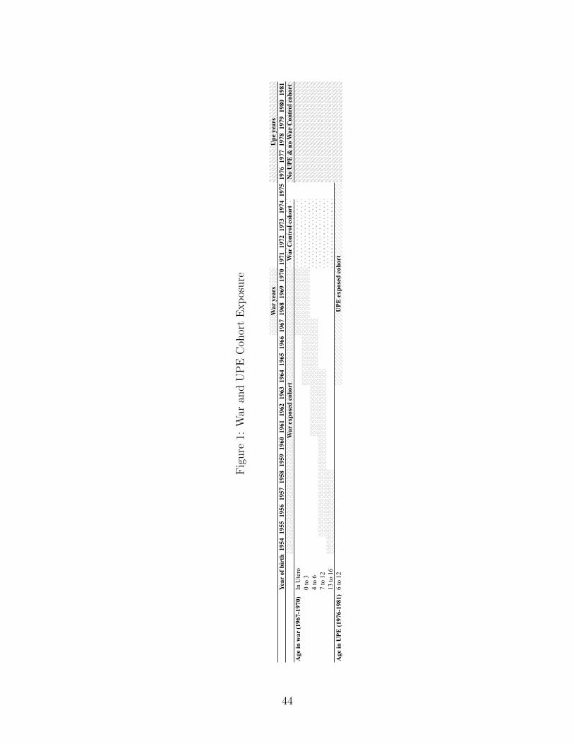
Fig

ure

1:W

aran

dU

PE

Coh

ort

Exp

osure

Ye

ar o

f bir

th19

5419

5519

5619

5719

5819

5919

6019

6119

6219

6319

6419

6519

6619

6719

6819

6919

7019

7119

7219

7319

7419

7519

7619

7719

7819

7919

8019

81

Age

in w

ar (1

967-

1970

)In

Ute

ro0

to 3

4 to

67

to 1

213

to 1

6A

ge in

UPE

(197

6-19

81)

6 to

12

UPE

exp

osed

coh

ort

War

yea

rsU

pe y

ears

War

exp

osed

coh

ort

War

Con

trol

coh

ort

No

UPE

& n

o W

ar C

ontr

ol c

ohor

t

44

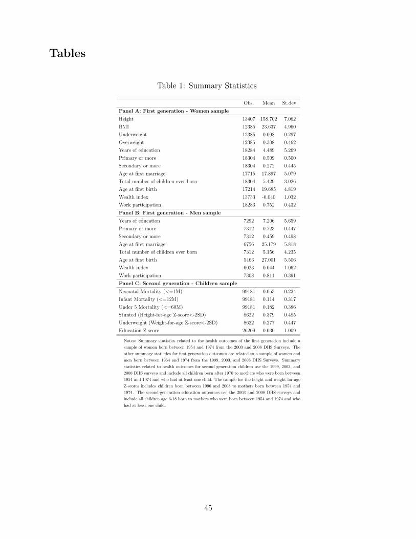
Tables

Table 1: Summary Statistics

Obs. Mean St.dev.

Panel A: First generation - Women sample

Height 13407 158.702 7.062

BMI 12385 23.637 4.960

Underweight 12385 0.098 0.297

Overweight 12385 0.308 0.462

Years of education 18284 4.489 5.269

Primary or more 18304 0.509 0.500

Secondary or more 18304 0.272 0.445

Age at first marriage 17715 17.897 5.079

Total number of children ever born 18304 5.429 3.026

Age at first birth 17214 19.685 4.819

Wealth index 13733 -0.040 1.032

Work participation 18283 0.752 0.432

Panel B: First generation - Men sample

Years of education 7292 7.206 5.659

Primary or more 7312 0.723 0.447

Secondary or more 7312 0.459 0.498

Age at first marriage 6756 25.179 5.818

Total number of children ever born 7312 5.156 4.235

Age at first birth 5463 27.001 5.506

Wealth index 6023 0.044 1.062

Work participation 7308 0.811 0.391

Panel C: Second generation - Children sample

Neonatal Mortality (<=1M) 99181 0.053 0.224

Infant Mortality (<=12M) 99181 0.114 0.317

Under 5 Mortality (<=60M) 99181 0.182 0.386

Stunted (Height-for-age Z-score<-2SD) 8622 0.379 0.485

Underweight (Weight-for-age Z-score<-2SD) 8622 0.277 0.447

Education Z score 26209 0.030 1.009

Notes: Summary statistics related to the health outcomes of the first generation include a

sample of women born between 1954 and 1974 from the 2003 and 2008 DHS Surveys. The

other summary statistics for first generation outcomes are related to a sample of women and

men born between 1954 and 1974 from the 1999, 2003, and 2008 DHS Surveys. Summary

statistics related to health outcomes for second generation children use the 1999, 2003, and

2008 DHS surveys and include all children born after 1970 to mothers who were born between

1954 and 1974 and who had at least one child. The sample for the height and weight-for-age

Z-scores includes children born between 1996 and 2008 to mothers born between 1954 and

1974. The second-generation education outcomes use the 2003 and 2008 DHS surveys and

include all children age 6-18 born to mothers who were born between 1954 and 1974 and who

had at least one child.

45

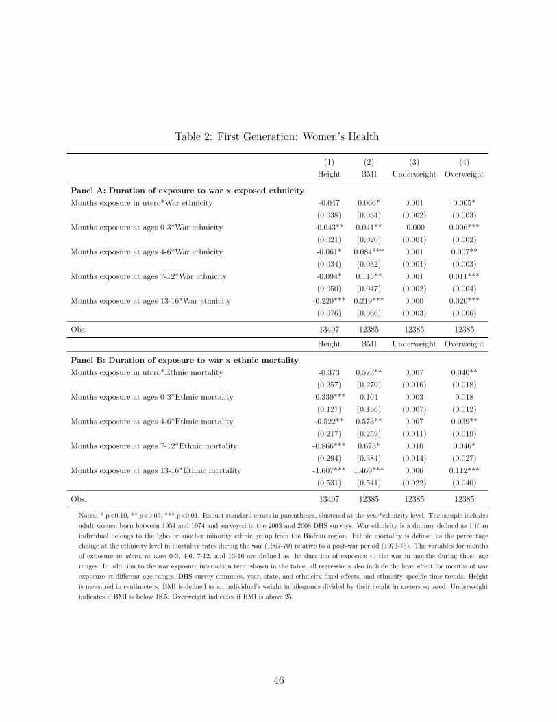
Table 2: First Generation: Women’s Health

(1) (2) (3) (4)

Height BMI Underweight Overweight

Panel A: Duration of exposure to war x exposed ethnicity

Months exposure in utero*War ethnicity -0.047 0.066* 0.001 0.005*

(0.038) (0.034) (0.002) (0.003)

Months exposure at ages 0-3*War ethnicity -0.043** 0.041** -0.000 0.006***

(0.021) (0.020) (0.001) (0.002)

Months exposure at ages 4-6*War ethnicity -0.061* 0.084*** 0.001 0.007**

(0.034) (0.032) (0.001) (0.003)

Months exposure at ages 7-12*War ethnicity -0.094* 0.115** 0.001 0.011***

(0.050) (0.047) (0.002) (0.004)

Months exposure at ages 13-16*War ethnicity -0.220*** 0.219*** 0.000 0.020***

(0.076) (0.066) (0.003) (0.006)

Obs. 13407 12385 12385 12385

Height BMI Underweight Overweight

Panel B: Duration of exposure to war x ethnic mortality

Months exposure in utero*Ethnic mortality -0.373 0.573** 0.007 0.040**

(0.257) (0.270) (0.016) (0.018)

Months exposure at ages 0-3*Ethnic mortality -0.339*** 0.164 0.003 0.018

(0.127) (0.156) (0.007) (0.012)

Months exposure at ages 4-6*Ethnic mortality -0.522** 0.573** 0.007 0.039**

(0.217) (0.259) (0.011) (0.019)

Months exposure at ages 7-12*Ethnic mortality -0.866*** 0.673* 0.010 0.046*

(0.294) (0.384) (0.014) (0.027)

Months exposure at ages 13-16*Ethnic mortality -1.607*** 1.469*** 0.006 0.112***

(0.531) (0.541) (0.022) (0.040)

Obs. 13407 12385 12385 12385

Notes: * p<0.10, ** p<0.05, *** p<0.01. Robust standard errors in parentheses, clustered at the year*ethnicity level. The sample includes

adult women born between 1954 and 1974 and surveyed in the 2003 and 2008 DHS surveys. War ethnicity is a dummy defined as 1 if an

individual belongs to the Igbo or another minority ethnic group from the Biafran region. Ethnic mortality is defined as the percentage

change at the ethnicity level in mortality rates during the war (1967-70) relative to a post-war period (1973-76). The variables for months

of exposure in utero, at ages 0-3, 4-6, 7-12, and 13-16 are defined as the duration of exposure to the war in months during those age

ranges. In addition to the war exposure interaction term shown in the table, all regressions also include the level effect for months of war

exposure at different age ranges, DHS survey dummies, year, state, and ethnicity fixed effects, and ethnicity specific time trends. Height

is measured in centimeters. BMI is defined as an individual’s weight in kilograms divided by their height in meters squared. Underweight

indicates if BMI is below 18.5. Overweight indicates if BMI is above 25.

46

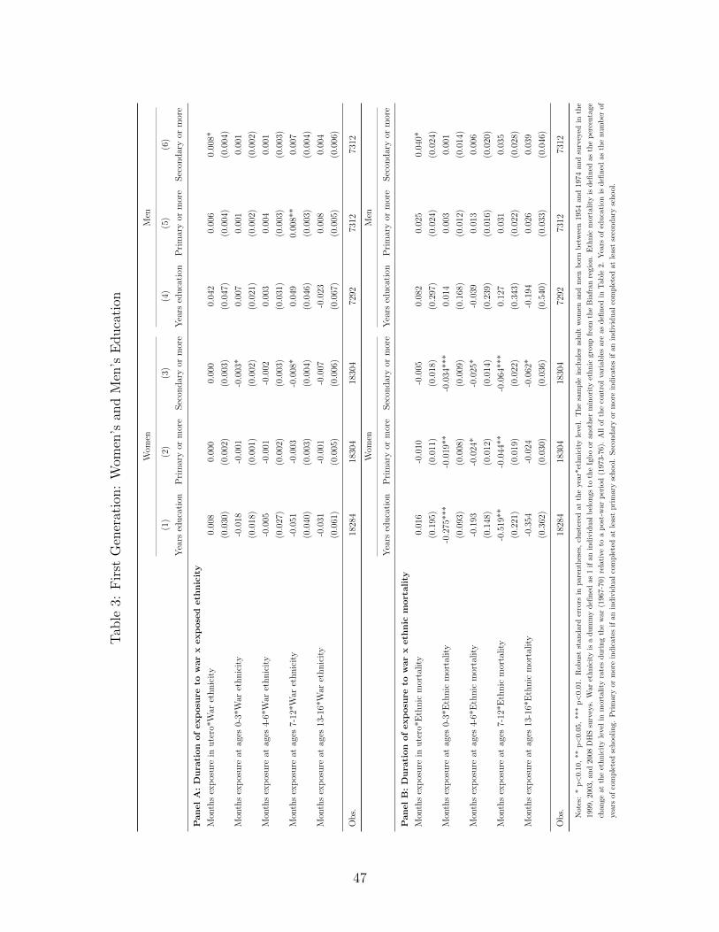
Tab

le3:

Fir

stG

ener

atio

n:

Wom

en’s

and

Men

’sE

duca

tion

Wom

enM

en

(1)

(2)

(3)

(4)

(5)

(6)

Yea

rsed

uca

tion

Pri

mar

yor

mor

eS

econ

dar

yor

mor

eY

ears

edu

cati

onP

rim

ary

orm

ore

Sec

ond

ary

orm

ore

Panel

A:

Dura

tion

of

exp

osu

reto

war

xexp

ose

deth

nic

ity

Mon

ths

exp

osu

rein

ute

ro*W

aret

hn

icit

y0.

008

0.00

00.

000

0.04

20.

006

0.00

8*

(0.0

30)

(0.0

02)

(0.0

03)

(0.0

47)

(0.0

04)

(0.0

04)

Mon

ths

exp

osu

reat

ages

0-3*

War

eth

nic

ity

-0.0

18-0

.001

-0.0

03*

0.00

70.

001

0.00

1

(0.0

18)

(0.0

01)

(0.0

02)

(0.0

21)

(0.0

02)

(0.0

02)

Mon

ths

exp

osu

reat

ages

4-6*

War

eth

nic

ity

-0.0

05-0

.001

-0.0

020.

003

0.00

40.

001

(0.0

27)

(0.0

02)

(0.0

03)

(0.0

31)

(0.0

03)

(0.0

03)

Mon

ths

exp

osu

reat

ages

7-12

*War

eth

nic

ity

-0.0

51-0

.003

-0.0

08*

0.04

90.

008*

*0.

007

(0.0

40)

(0.0

03)

(0.0

04)

(0.0

46)

(0.0

03)

(0.0

04)

Mon

ths

exp

osu

reat

ages

13-1

6*W

aret

hn

icit

y-0

.031

-0.0

01-0

.007

-0.0

230.

008

0.00

4

(0.0

61)

(0.0

05)

(0.0

06)

(0.0

67)

(0.0

05)

(0.0

06)

Ob

s.18

284

1830

418

304

7292

7312

7312

Wom

enM

en

Yea

rsed

uca

tion

Pri

mar

yor

mor

eS

econ

dar

yor

mor

eY

ears

edu

cati

onP

rim

ary

orm

ore

Sec

ond

ary

orm

ore

Panel

B:

Dura

tion

of

exp

osu

reto

war

xeth

nic

mort

ality

Mon

ths

exp

osu

rein

ute

ro*E

thn

icm

orta

lity

0.01

6-0

.010

-0.0

050.

082

0.02

50.

040*

(0.1

95)

(0.0

11)

(0.0

18)

(0.2

97)

(0.0

24)

(0.0

24)

Mon

ths

exp

osu

reat

ages

0-3*

Eth

nic

mor

tali

ty-0

.275

***

-0.0

19**

-0.0

34**

*0.

014

0.00

30.

001

(0.0

93)

(0.0

08)

(0.0

09)

(0.1

68)

(0.0

12)

(0.0

14)

Mon

ths

exp

osu

reat

ages

4-6*

Eth

nic

mor

tali

ty-0

.193

-0.0

24*

-0.0

25*

-0.0

390.

013

0.00

6

(0.1

48)

(0.0

12)

(0.0

14)

(0.2

39)

(0.0

16)

(0.0

20)

Mon

ths

exp

osu

reat

ages

7-12

*Eth

nic

mor

tali

ty-0

.519

**-0

.044

**-0

.064

***

0.12

70.

031

0.03

5

(0.2

21)

(0.0

19)

(0.0

22)

(0.3

43)

(0.0

22)

(0.0

28)

Mon

ths

exp

osu

reat

ages

13-1

6*E

thn

icm

orta

lity

-0.3

54-0

.024

-0.0

62*

-0.1

940.

026

0.03

9

(0.3

62)

(0.0

30)

(0.0

36)

(0.5

40)

(0.0

33)

(0.0

46)

Ob

s.18

284

1830

418

304

7292

7312

7312

Not

es:

*p<

0.10

,**

p<

0.05

,**

*p<

0.01

.R

obust

standar

der

rors

inpar

enth

eses

,cl

ust

ered

at

the

year

*eth

nic

ity

leve

l.T

he

sam

ple

incl

udes

adult

wom

enan

dm

enb

orn

bet

wee

n195

4and

1974

and

surv

eyed

inth

e

199

9,20

03,

and

2008

DH

Ssu

rvey

s.W

aret

hnic

ity

isa

dum

my

defi

ned

as

1if

anin

div

idual

bel

ongs

toth

eIg

bo

oran

other

min

orit

yet

hnic

grou

pfr

omth

eB

iafr

an

regi

on.

Eth

nic

mor

tality

isdefi

ned

as

the

per

centa

ge

chan

geat

the

ethnic

ity

leve

lin

mor

tality

rate

sduri

ng

the

war

(196

7-70

)re

lati

veto

ap

ost-

war

per

iod

(197

3-7

6).

All

ofth

eco

ntr

olva

riab

les

are

asdefi

ned

inT

able

2.

Yea

rsof

educa

tion

isdefi

ned

as

the

nu

mb

erof

year

sof

com

ple

ted

school

ing.

Pri

mar

yor

mor

ein

dic

ates

ifan

indiv

idual

com

ple

ted

atle

ast

pri

mar

ysc

hool

.Sec

ondar

yor

mor

ein

dic

ate

sif

anin

div

idual

com

ple

ted

atle

ast

seco

ndary

school.

47

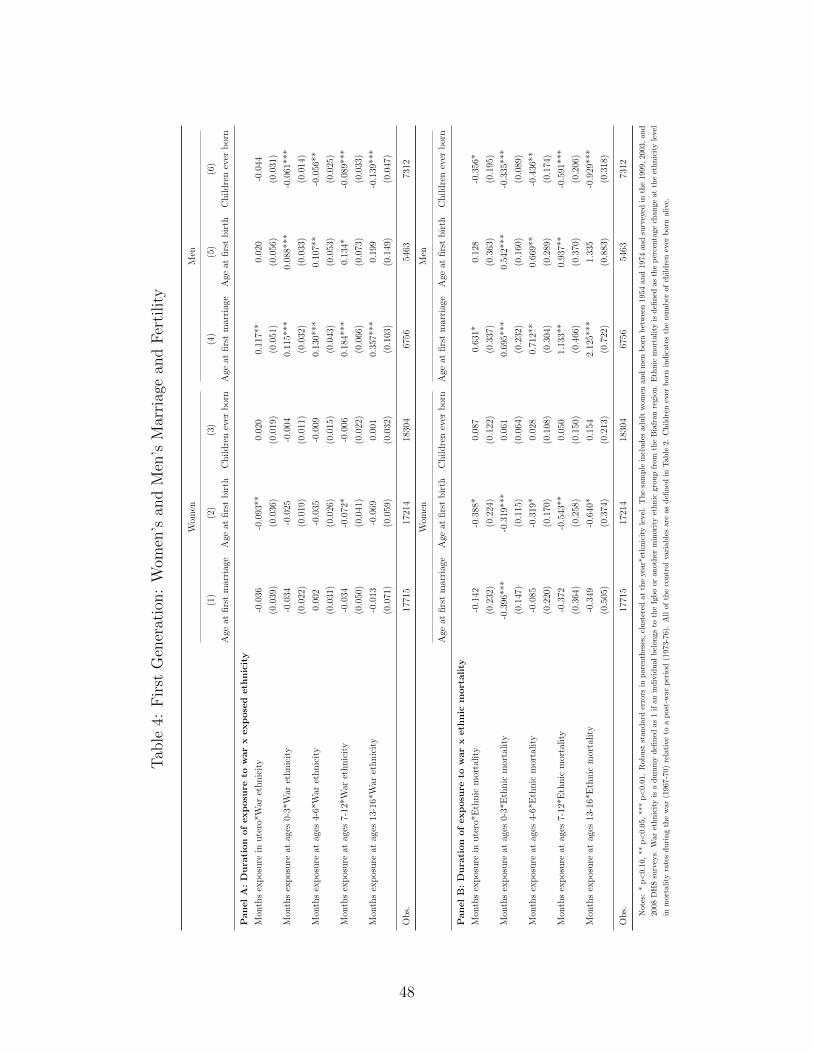
Tab

le4:

Fir

stG

ener

atio

n:

Wom

en’s

and

Men

’sM

arri

age

and

Fer

tility

Wom

enM

en

(1)

(2)

(3)

(4)

(5)

(6)

Age

atfi

rst

mar

riag

eA

geat

firs

tb

irth

Ch

ild

ren

ever

bor

nA

geat

firs

tm

arri

age

Age

atfi

rst

bir

thC

hil

dre

nev

erb

orn

Pan

el

A:

Du

rati

on

of

exp

osu

reto

war

xexp

ose

deth

nic

ity

Mon

ths

exp

osu

rein

ute

ro*W

aret

hn

icit

y-0

.036

-0.0

93**

0.02

00.

117*

*0.

020

-0.0

44

(0.0

39)

(0.0

36)

(0.0

19)

(0.0

51)

(0.0

56)

(0.0

31)

Mon

ths

exp

osu

reat

ages

0-3*

War

eth

nic

ity

-0.0

34-0

.025

-0.0

040.

115*

**0.

088*

**-0

.061

***

(0.0

22)

(0.0

19)

(0.0

11)

(0.0

32)

(0.0

33)

(0.0

14)

Mon

ths

exp

osu

reat

ages

4-6*

War

eth

nic

ity

0.00

2-0

.035

-0.0

090.

130*

**0.

107*

*-0

.056

**

(0.0

31)

(0.0

26)

(0.0

15)

(0.0

43)

(0.0

53)

(0.0

25)

Mon

ths

exp

osu

reat

ages

7-12

*War

eth

nic

ity

-0.0

34-0

.072

*-0

.006

0.18

4***

0.13

4*-0

.089

***

(0.0

50)

(0.0

41)

(0.0

22)

(0.0

66)

(0.0

73)

(0.0

33)

Mon

ths

exp

osu

reat

ages

13-1

6*W

aret

hn

icit

y-0

.013

-0.0

690.

001

0.35

7***

0.19

9-0

.139

***

(0.0

71)

(0.0

59)

(0.0

32)

(0.1

03)

(0.1

49)

(0.0

47)

Ob

s.17

715

1721

418

304

6756

5463

7312

Wom

enM

en

Age

atfi

rst

mar

riag

eA

geat

firs

tb

irth

Ch

ild

ren

ever

bor

nA

geat

firs

tm

arri

age

Age

atfi

rst

bir

thC

hil

dre

nev

erb

orn

Pan

el

B:

Du

rati

on

of

exp

osu

reto

war

xeth

nic

mort

ali

ty

Mon

ths

exp

osu

rein

ute

ro*E

thn

icm

orta

lity

-0.1

42-0

.388

*0.

087

0.63

1*0.

128

-0.3

56*

(0.2

32)

(0.2

24)

(0.1

22)

(0.3

37)

(0.3

63)

(0.1

95)

Mon

ths

exp

osu

reat

ages

0-3*

Eth

nic

mor

tali

ty-0

.396

***

-0.3

19**

*0.

061

0.69

5***

0.54

2***

-0.3

35**

*

(0.1

47)

(0.1

15)

(0.0

64)

(0.2

32)

(0.1

60)

(0.0

89)

Mon

ths

exp

osu

reat

ages

4-6*

Eth

nic

mor

tali

ty-0

.085

-0.3

19*

0.02

80.

712*

*0.

669*

*-0

.436

**

(0.2

20)

(0.1

70)

(0.1

08)

(0.3

04)

(0.2

89)

(0.1

74)

Mon

ths

exp

osu

reat

ages

7-12

*Eth

nic

mor

tali

ty-0

.372

-0.5

43**

0.05

01.

133*

*0.

937*

*-0

.591

***

(0.3

64)

(0.2

58)

(0.1

50)

(0.4

66)

(0.3

70)

(0.2

06)

Mon

ths

exp

osu

reat

ages

13-1

6*E

thn

icm

orta

lity

-0.3

49-0

.640

*0.

154

2.12

5***

1.33

5-0

.929

***

(0.5

05)

(0.3

74)

(0.2

13)

(0.7

22)

(0.8

83)

(0.3

18)

Ob

s.17

715

1721

418

304

6756

5463

7312

Not

es:

*p<

0.10

,**

p<

0.05

,**

*p<

0.01

.R

ob

ust

stan

dard

erro

rsin

pare

nth

eses

,cl

ust

ered

atth

eye

ar*

eth

nic

ity

leve

l.T

he

sam

ple

incl

udes

ad

ult

wom

enan

dm

enb

orn

bet

wee

n195

4an

d197

4an

dsu

rvey

edin

the

1999

,200

3,an

d

200

8D

HS

surv

eys.

War

eth

nic

ity

isa

du

mm

yd

efin

edas

1if

anin

div

idu

al

bel

ongs

toth

eIg

bo

or

an

oth

erm

inor

ity

eth

nic

grou

pfr

om

the

Bia

fran

regi

on.

Eth

nic

mor

tali

tyis

defi

ned

asth

ep

erce

nta

ge

chan

ge

atth

eet

hn

icit

yle

vel

inm

orta

lity

rate

sd

uri

ng

the

war

(196

7-70)

rela

tive

toa

pos

t-w

arp

erio

d(1

973-7

6).

All

of

the

contr

ol

vari

ab

les

are

asd

efin

edin

Tab

le2.

Ch

ild

ren

ever

born

ind

icate

sth

enu

mb

erof

chil

dre

nev

erb

orn

ali

ve.

48

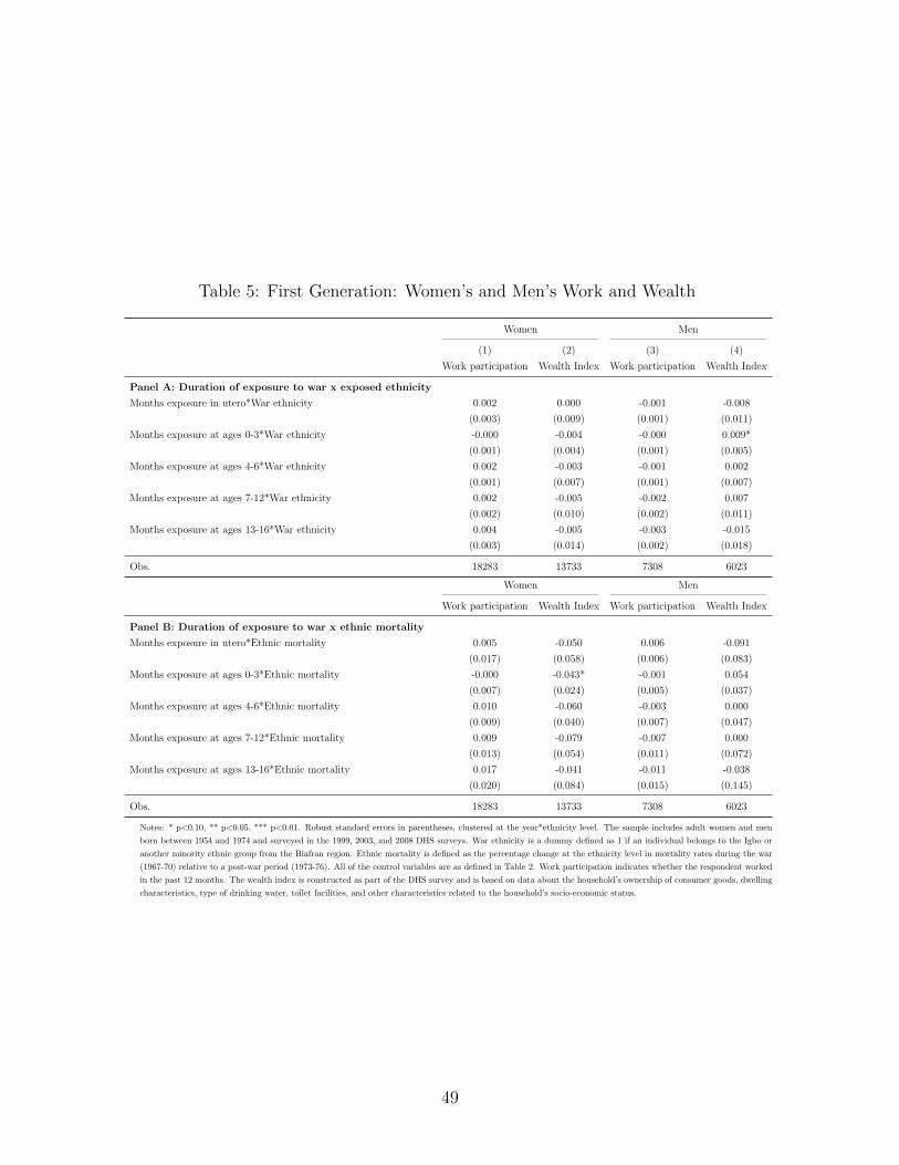
Table 5: First Generation: Women’s and Men’s Work and Wealth

Women Men

(1) (2) (3) (4)

Work participation Wealth Index Work participation Wealth Index

Panel A: Duration of exposure to war x exposed ethnicity

Months exposure in utero*War ethnicity 0.002 0.000 -0.001 -0.008

(0.003) (0.009) (0.001) (0.011)

Months exposure at ages 0-3*War ethnicity -0.000 -0.004 -0.000 0.009*

(0.001) (0.004) (0.001) (0.005)

Months exposure at ages 4-6*War ethnicity 0.002 -0.003 -0.001 0.002

(0.001) (0.007) (0.001) (0.007)

Months exposure at ages 7-12*War ethnicity 0.002 -0.005 -0.002 0.007

(0.002) (0.010) (0.002) (0.011)

Months exposure at ages 13-16*War ethnicity 0.004 -0.005 -0.003 -0.015

(0.003) (0.014) (0.002) (0.018)

Obs. 18283 13733 7308 6023

Women Men

Work participation Wealth Index Work participation Wealth Index

Panel B: Duration of exposure to war x ethnic mortality

Months exposure in utero*Ethnic mortality 0.005 -0.050 0.006 -0.091

(0.017) (0.058) (0.006) (0.083)

Months exposure at ages 0-3*Ethnic mortality -0.000 -0.043* -0.001 0.054

(0.007) (0.024) (0.005) (0.037)

Months exposure at ages 4-6*Ethnic mortality 0.010 -0.060 -0.003 0.000

(0.009) (0.040) (0.007) (0.047)

Months exposure at ages 7-12*Ethnic mortality 0.009 -0.079 -0.007 0.000

(0.013) (0.054) (0.011) (0.072)

Months exposure at ages 13-16*Ethnic mortality 0.017 -0.041 -0.011 -0.038

(0.020) (0.084) (0.015) (0.145)

Obs. 18283 13733 7308 6023

Notes: * p<0.10, ** p<0.05, *** p<0.01. Robust standard errors in parentheses, clustered at the year*ethnicity level. The sample includes adult women and men

born between 1954 and 1974 and surveyed in the 1999, 2003, and 2008 DHS surveys. War ethnicity is a dummy defined as 1 if an individual belongs to the Igbo or

another minority ethnic group from the Biafran region. Ethnic mortality is defined as the percentage change at the ethnicity level in mortality rates during the war

(1967-70) relative to a post-war period (1973-76). All of the control variables are as defined in Table 2. Work participation indicates whether the respondent worked

in the past 12 months. The wealth index is constructed as part of the DHS survey and is based on data about the household’s ownership of consumer goods, dwelling

characteristics, type of drinking water, toilet facilities, and other characteristics related to the household’s socio-economic status.

49

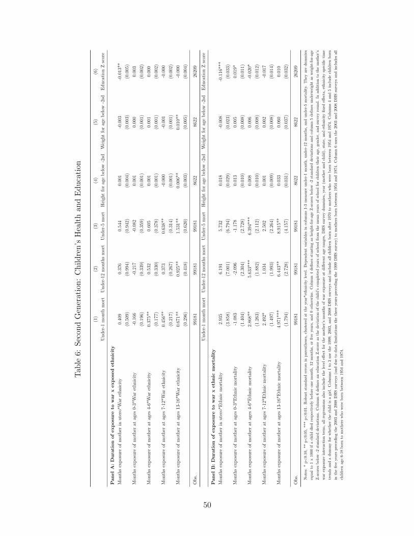
Tab

le6:

Sec

ond

Gen

erat

ion:

Childre

n’s

Hea

lth

and

Educa

tion

(1)

(2)

(3)

(4)

(5)

(6)

Un

der

-1m

onth

mor

tU

nd

er-1

2m

onth

sm

ort

Un

der

-5m

ort

Hei

ght

for

age

bel

ow-2

sdW

eigh

tfo

rag

eb

elow

-2sd

Ed

uca

tion

Zsc

ore

Pan

el

A:

Du

rati

on

of

exp

osu

reto

war

xexp

ose

deth

nic

ity

Mon

ths

exp

osu

reof

mot

her

inu

tero

*War

eth

nic

ity

0.40

90.

376

0.54

40.

001

-0.0

03-0

.013

**

(0.5

09)

(0.9

94)

(0.9

42)

(0.0

04)

(0.0

03)

(0.0

05)

Mon

ths

exp

osu

reof

mot

her

atag

es0-

3*W

aret

hn

icit

y-0

.166

-0.2

17-0

.082

0.00

10.

000

0.00

3

(0.1

96)

(0.3

39)

(0.3

59)

(0.0

01)

(0.0

01)

(0.0

02)

Mon

ths

exp

osu

reof

mot

her

atag

es4-

6*W

aret

hn

icit

y0.

375*

*0.

532

0.60

50.

001

0.00

10.

000

(0.1

77)

(0.3

30)

(0.3

78)

(0.0

01)

(0.0

01)

(0.0

02)

Mon

ths

exp

osu

reof

mot

her

atag

es7-

12*W

aret

hn

icit

y0.

456*

*0.

373

0.63

8**

-0.0

00-0

.001

-0.0

00

(0.2

17)

(0.2

67)

(0.3

14)

(0.0

01)

(0.0

01)

(0.0

02)

Mon

ths

exp

osu

reof

mot

her

atag

es13

-16*

War

eth

nic

ity

0.67

1**

0.92

5**

1.53

1**

0.00

6**

0.01

0**

-0.0

00

(0.2

96)

(0.4

18)

(0.6

20)

(0.0

03)

(0.0

05)

(0.0

04)

Ob

s.99

181

9918

199

181

8622

8622

2620

9

Un

der

-1m

onth

mor

tU

nd

er-1

2m

onth

sm

ort

Un

der

-5m

ort

Hei

ght

for

age

bel

ow-2

sdW

eigh

tfo

rag

eb

elow

-2sd

Ed

uca

tion

Zsc

ore

Pan

el

B:

Du

rati

on

of

exp

osu

reto

war

xeth

nic

mort

ali

ty

Mon

ths

exp

osu

reof

mot

her

inu

tero

*Eth

nic

mor

tality

2.93

56.

191

5.73

20.

018

-0.0

08-0

.116

***

(3.8

58)

(7.0

01)

(6.7

94)

(0.0

29)

(0.0

23)

(0.0

33)

Mon

ths

exp

osu

reof

mot

her

atag

es0-

3*E

thn

icm

orta

lity

-1.0

83-2

.096

-1.1

780.

013

0.00

50.

019*

(1.4

04)

(2.3

04)

(2.7

28)

(0.0

10)

(0.0

08)

(0.0

11)

Mon

ths

exp

osu

reof

mot

her

atag

es4-

6*E

thn

icm

orta

lity

2.86

8**

5.63

3***

6.39

4***

0.00

80.

006

-0.0

20*

(1.2

63)

(1.8

82)

(2.1

12)

(0.0

10)

(0.0

08)

(0.0

12)

Mon

ths

exp

osu

reof

mot

her

atag

es7-

12*E

thn

icm

orta

lity

2.49

2*1.

034

2.50

20.

001

0.00

2-0

.017

(1.4

97)

(1.9

93)

(2.2

64)

(0.0

09)

(0.0

08)

(0.0

14)

Mon

ths

exp

osu

reof

mot

her

atag

es13

-16*

Eth

nic

mor

tali

ty4.

971*

**6.

443*

*8.

915*

*0.

033

0.06

00.

010

(1.7

94)

(2.7

28)

(4.1

57)

(0.0

31)

(0.0

37)

(0.0

32)

Ob

s.99

181

9918

199

181

8622

8622

2620

9

Not

es:

*p<

0.10

,**

p<

0.05

,**

*p<

0.01

.R

obu

stst

an

dar

der

rors

inp

are

nth

eses

,cl

ust

ered

at

the

year

*eth

nic

ity

leve

l.D

epen

den

tva

riab

les

inco

lum

ns

1-3

mea

sure

un

der

-1m

onth

,un

der

-12

mon

ths,

and

un

der

-5m

orta

lity

.T

hey

are

du

mm

ies

equ

alto

1x

1000

ifa

chil

dd

ied

resp

ecti

vely

bef

ore

on

em

onth

,12

mon

ths,

or

five

years

,an

d0

oth

erw

ise.

Colu

mn

4d

efin

esst

unti

ng

ash

eigh

t-fo

r-ag

eZ

-sco

res

bel

ow-2

stan

dar

ddev

iati

ons

and

colu

mn

5defi

nes

un

der

wei

ght

as

wei

ght-

for-

age

Z-s

core

sb

elow

-2st

and

ard

dev

iati

ons.

Col

um

n6

defi

nes

aned

uca

tion

Z-s

core

as

the

dev

iati

on

of

the

chil

d’s

com

ple

ted

year

sof

sch

ool

from

the

mea

nye

ars

of

sch

ool

for

chil

dre

nth

eir

age,

gen

der

,an

dsu

rvey

rou

nd

.In

ad

dit

ion

toth

em

oth

er’s

war

exp

osu

rein

tera

ctio

nte

rm,

all

regr

essi

ons

als

oin

clu

de

the

level

effec

tfo

rth

em

oth

er’s

month

sof

war

exp

osu

reat

diff

eren

tag

era

nge

s,D

HS

surv

eyd

um

mie

s,yea

r(m

oth

eran

dch

ild

),st

ate,

and

eth

nic

ity

fixed

effec

ts,

eth

nic

ity

spec

ific

tim

e

tren

ds

and

ad

um

my

for

wh

eth

erth

ech

ild

isa

girl

.C

olu

mn

s1

to3

use

the

1999,

2003

,an

d2008

DH

Ssu

rvey

san

din

clu

de

all

chil

dre

nb

orn

afte

r197

0to

moth

ers

wh

ow

ere

bor

nb

etw

een

1954

and

1974

.C

olu

mn

s4

and

5in

clu

de

chil

dre

nb

orn

inth

efi

veye

ars

pre

ced

ing

the

2003

and

2008

DH

Ssu

rvey

s(a

nd

du

eto

dat

ali

mit

ati

on

sth

eth

ree

years

pre

ced

ing

the

1999

DH

Ssu

rvey

)to

moth

ers

bor

nb

etw

een

195

4an

d19

74.

Col

um

n6

use

sth

e20

03an

d20

08D

HS

surv

eys

and

incl

ud

esal

l

chil

dre

nag

e6-

18b

orn

tom

oth

ers

wh

ow

ere

bor

nb

etw

een

1954

and

1974.

50

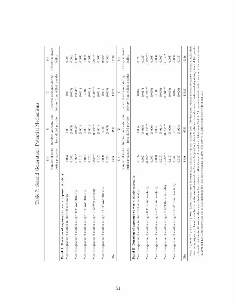
Tab

le7:

Sec

ond

Gen

erat

ion:

Pot

enti

alM

echan

ism

s

(1)

(2)

(3)

(4)

Nu

mb

erof

vis

its

Rec

eive

dan

ten

atal

care

Rec

eive

das

sist

ance

du

rin

gD

eliv

ery

inh

ealt

h

du

rin

gp

regn

ancy

from

skil

led

pro

vid

erd

eliv

ery

from

skil

led

pro

vid

erfa

cili

ty

Panel

A:

Dura

tion

of

exp

osu

reto

war

xexp

ose

deth

nic

ity

Mon

ths

exp

osu

reof

mot

her

inute

ro*W

aret

hn

icit

y-0

.033

0.00

10.

001

0.00

3

(0.0

42)

(0.0

03)

(0.0

03)

(0.0

04)

Mon

ths

exp

osu

reof

mot

her

atag

es0-

3*W

aret

hn

icit

y-0

.027

**-0

.003

**-0

.003

**-0

.003

**

(0.0

13)

(0.0

01)

(0.0

01)

(0.0

01)

Mon

ths

exp

osu

reof

mot

her

atag

es4-

6*W

aret

hn

icit

y-0

.014

0.00

1-0

.001

-0.0

02

(0.0

24)

(0.0

01)

(0.0

01)

(0.0

01)

Mon

ths

exp

osu

reof

mot

her

atag

es7-

12*W

aret

hn

icit

y-0

.070

***

-0.0

04**

*-0

.006

***

-0.0

04**

*

(0.0

15)

(0.0

01)

(0.0

01)

(0.0

01)

Mon

ths

exp

osu

reof

mot

her

atag

es13

-16*

War

eth

nic

ity

-0.0

09-0

.000

0.00

4-0

.006

*

(0.0

34)

(0.0

03)

(0.0

03)

(0.0

03)

Ob

s.88

3995

5613

322

1323

6

(1)

(2)

(3)

(4)

Nu

mb

erof

vis

its

Rec

eive

dan

ten

atal

care

Rec

eive

das

sist

ance

du

rin

gD

eliv

ery

inh

ealt

h

du

rin

gp

regn

ancy

from

skil

led

pro

vid

erd

eliv

ery

from

skil

led

pro

vid

erfa

cili

ty

Panel

B:

Dura

tion

of

exp

osu

reto

war

xeth

nic

mort

ality

Mon

ths

exp

osu

reof

mot

her

inute

ro*E

thn

icm

orta

lity

-0.1

650.

005

0.01

60.

029

(0.3

62)

(0.0

15)

(0.0

17)

(0.0

27)

Mon

ths

exp

osu

reof

mot

her

atag

es0-

3*E

thn

icm

orta

lity

-0.1

85*

-0.0

23**

*-0

.021

***

-0.0

23**

*

(0.0

95)

(0.0

06)

(0.0

06)

(0.0

08)

Mon

ths

exp

osu

reof

mot

her

atag

es4-

6*E

thn

icm

orta

lity

-0.0

830.

004

-0.0

09-0

.006

(0.2

16)

(0.0

11)

(0.0

06)

(0.0

07)

Mon

ths

exp

osu

reof

mot

her

atag

es7-

12*E

thn

icm

orta

lity

-0.4

53**

*-0

.029

***

-0.0

34**

*-0

.017

**

(0.1

16)

(0.0

09)

(0.0

09)

(0.0

08)

Mon

ths

exp

osu

reof

mot

her

atag

es13

-16*

Eth

nic

mor

tali

ty0.

047

-0.0

130.

015

-0.0

38

(0.3

32)

(0.0

24)

(0.0

26)

(0.0

33)

Ob

s.88

3995

5613

322

1323

6

Not

es:

*p<

0.10

,**

p<

0.05,

***

p<

0.01

.R

obust

standard

erro

rsin

par

enth

eses

,cl

ust

ered

atth

eye

ar*e

thnic

ity

leve

l.T

he

dep

enden

tva

riab

les

mea

sure

the

num

ber

of

pre

nata

lhea

lth

clin

ic

vis

its

duri

ng

pre

gnan

cy(c

olum

n1)

,w

het

her

the

mot

her

rece

ived

ante

nat

alca

refr

oma

skille

dpro

vid

er(c

olum

n2)

,w

het

her

the

mot

her

rece

ived

ass

ista

nce

du

ring

del

iver

yfr

om

ask

ille

dpro

vid

er

(col

um

n3)

,an

dw

het

her

the

mot

her

del

iver

edin

ahea

lth

faci

lity

(col

um

n4)

.A

llof

the

contr

ol

vari

able

sar

edefi

ned

asin

Tab

le6.

All

regre

ssio

ns

incl

ude

childre

nb

orn

inth

efive

year

sp

rece

din

g

the

2003

and

2008

DH

Ssu

rvey

s(a

nd

due

todat

alim

itat

ions

the

thre

eyea

rspre

cedin

gth

e19

99D

HS

surv

ey)

tom

other

sb

orn

bet

wee

n195

4an

d197

4.

51

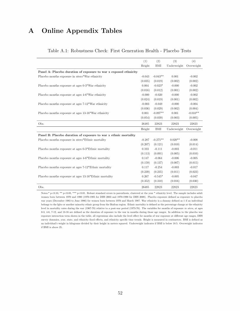
A Online Appendix Tables

Table A.1: Robustness Check: First Generation Health - Placebo Tests

(1) (2) (3) (4)

Height BMI Underweight Overweight

Panel A: Placebo duration of exposure to war x exposed ethnicity

Placebo months exposure in utero*War ethnicity -0.043 -0.043** 0.001 -0.002

(0.035) (0.019) (0.002) (0.002)

Placebo months exposure at ages 0-3*War ethnicity 0.004 -0.023* -0.000 -0.002

(0.016) (0.012) (0.001) (0.002)

Placebo months exposure at ages 4-6*War ethnicity -0.000 -0.020 -0.000 -0.002

(0.024) (0.019) (0.001) (0.002)

Placebo months exposure at ages 7-12*War ethnicity -0.003 -0.049 -0.000 -0.004

(0.036) (0.029) (0.002) (0.004)

Placebo months exposure at ages 13-16*War ethnicity 0.001 -0.097** 0.001 -0.010**

(0.054) (0.039) (0.003) (0.005)

Obs. 26485 22823 22823 22823

Height BMI Underweight Overweight

Panel B: Placebo duration of exposure to war x ethnic mortality

Placebo months exposure in utero*Ethnic mortality -0.287 -0.275** 0.020** -0.008

(0.207) (0.121) (0.010) (0.014)

Placebo months exposure at ages 0-3*Ethnic mortality 0.103 -0.111 -0.003 -0.011

(0.113) (0.091) (0.005) (0.010)

Placebo months exposure at ages 4-6*Ethnic mortality 0.147 -0.064 -0.006 -0.005

(0.159) (0.137) (0.007) (0.015)

Placebo months exposure at ages 7-12*Ethnic mortality 0.117 -0.254 -0.003 -0.017

(0.239) (0.235) (0.011) (0.023)

Placebo months exposure at ages 13-16*Ethnic mortality 0.267 -0.545* -0.005 -0.047

(0.352) (0.310) (0.016) (0.030)

Obs. 26485 22823 22823 22823

Notes:* p<0.10, ** p<0.05, *** p<0.01. Robust standard errors in parenthesis, clustered at the year * ethnicity level. The sample includes adult

women born between 1970 and 1990 (1970-1985 for DHS 2003 and 1970-1990 for DHS 2008). Placebo exposure defined as exposure to placebo

war years (December 1983 to June 1986) for women born between 1970 and March 1987. War ethnicity is a dummy defined as 1 if an individual

belongs to the Igbo or another minority ethnic group from the Biafran region. Ethnic mortality is defined as the percentage change at the ethnicity

level in mortality rates during the war (1967-70) relative to a post-war period (1973-76). The variables for months of exposure in utero, at ages

0-3, 4-6, 7-12, and 13-16 are defined as the duration of exposure to the war in months during those age ranges. In addition to the placebo war

exposure interaction term shown in the table, all regressions also include the level effect for months of war exposure at different age ranges, DHS

survey dummies, year, state, and ethnicity fixed effects, and ethnicity specific time trends. Height is measured in centimeters. BMI is defined as

an individual’s weight in kilograms divided by their height in meters squared. Underweight indicates if BMI is below 18.5. Overweight indicates

if BMI is above 25.

52

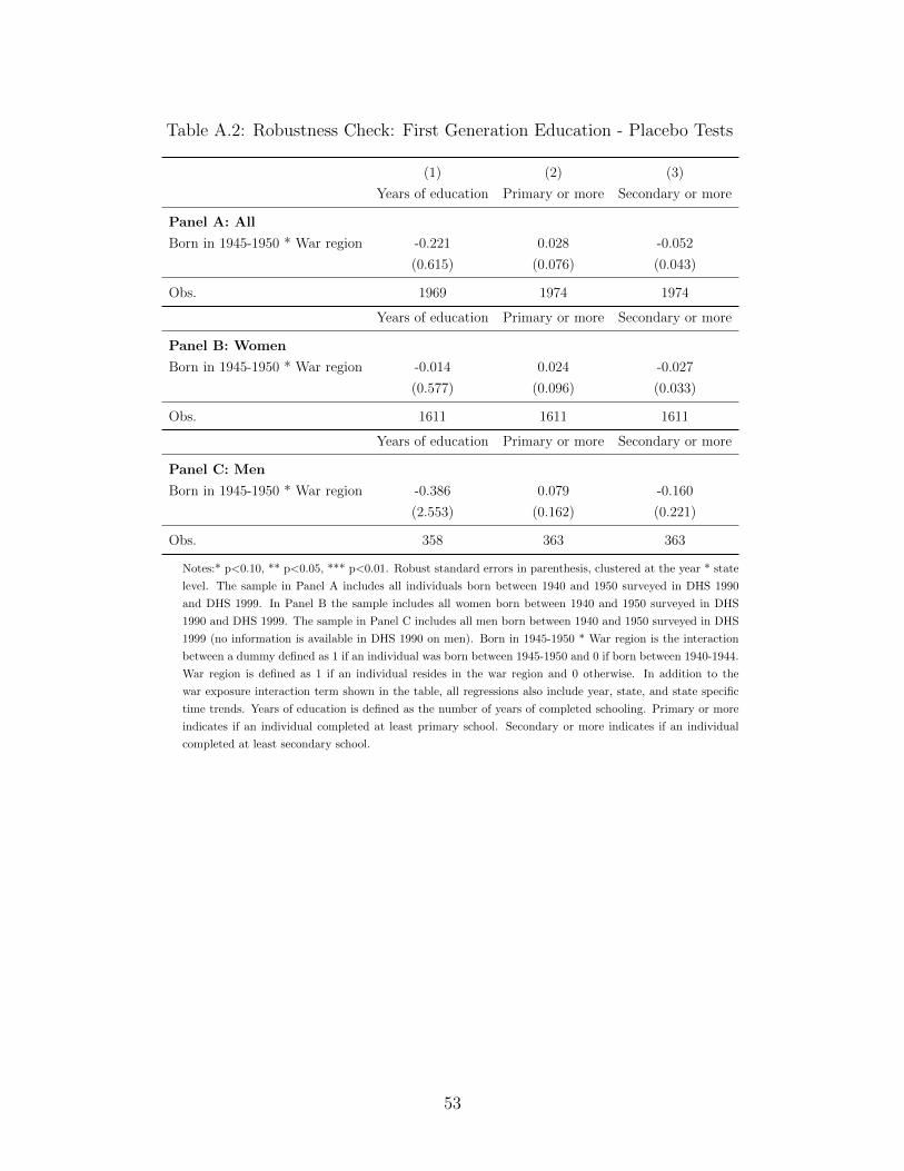
Table A.2: Robustness Check: First Generation Education - Placebo Tests

(1) (2) (3)

Years of education Primary or more Secondary or more

Panel A: All

Born in 1945-1950 * War region -0.221 0.028 -0.052

(0.615) (0.076) (0.043)

Obs. 1969 1974 1974

Years of education Primary or more Secondary or more

Panel B: Women

Born in 1945-1950 * War region -0.014 0.024 -0.027

(0.577) (0.096) (0.033)

Obs. 1611 1611 1611

Years of education Primary or more Secondary or more

Panel C: Men

Born in 1945-1950 * War region -0.386 0.079 -0.160

(2.553) (0.162) (0.221)

Obs. 358 363 363

Notes:* p<0.10, ** p<0.05, *** p<0.01. Robust standard errors in parenthesis, clustered at the year * state

level. The sample in Panel A includes all individuals born between 1940 and 1950 surveyed in DHS 1990

and DHS 1999. In Panel B the sample includes all women born between 1940 and 1950 surveyed in DHS

1990 and DHS 1999. The sample in Panel C includes all men born between 1940 and 1950 surveyed in DHS

1999 (no information is available in DHS 1990 on men). Born in 1945-1950 * War region is the interaction

between a dummy defined as 1 if an individual was born between 1945-1950 and 0 if born between 1940-1944.

War region is defined as 1 if an individual resides in the war region and 0 otherwise. In addition to the

war exposure interaction term shown in the table, all regressions also include year, state, and state specific

time trends. Years of education is defined as the number of years of completed schooling. Primary or more

indicates if an individual completed at least primary school. Secondary or more indicates if an individual

completed at least secondary school.

53

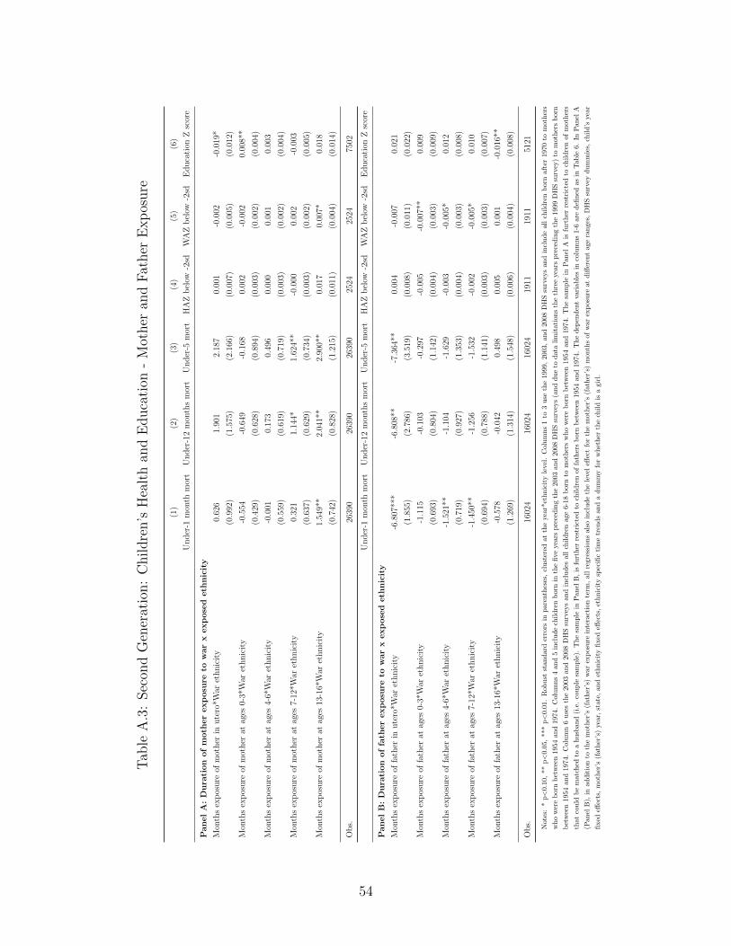
Tab

leA

.3:

Sec

ond

Gen

erat

ion:

Childre

n’s

Hea

lth

and

Educa

tion

-M

other

and

Fat

her

Exp

osure

(1)

(2)

(3)

(4)

(5)

(6)

Un

der

-1m

onth

mor

tU

nd

er-1

2m

onth

sm

ort

Un

der

-5m

ort

HA

Zb

elow

-2sd

WA

Zb

elow

-2sd

Ed

uca

tion

Zsc

ore

Pan

el

A:

Du

rati

on

of

moth

er

exp

osu

reto

war

xexp

ose

deth

nic

ity

Mon

ths

exp

osu

reof

mot

her

inute

ro*W

aret

hn

icit

y0.

626

1.90

12.

187

0.00

1-0

.002

-0.0

19*

(0.9

92)

(1.5

75)

(2.1

66)

(0.0

07)

(0.0

05)

(0.0

12)

Mon

ths

exp

osu

reof

mot

her

atag

es0-

3*W

aret

hn

icit

y-0

.554

-0.6

49-0

.168

0.00

2-0

.002

0.00

8**

(0.4

29)

(0.6

28)

(0.8

94)

(0.0

03)

(0.0

02)

(0.0

04)

Mon

ths

exp

osu

reof

mot

her

atag

es4-

6*W

aret

hn

icit

y-0

.001

0.17

30.

496

0.00

00.

001

0.00

3

(0.5

59)

(0.6

19)

(0.7

19)

(0.0

03)

(0.0

02)

(0.0

04)

Mon

ths

exp

osu

reof

mot

her

atag

es7-

12*W

aret

hn

icit

y0.

321

1.14

4*1.

624*

*-0

.000

0.00

2-0

.003

(0.6

37)

(0.6

29)

(0.7

34)

(0.0

03)

(0.0

02)

(0.0

05)

Mon

ths

exp

osu

reof

mot

her

atag

es13

-16*

War

eth

nic

ity

1.54

9**

2.04

1**

2.90

0**

0.01

70.

007*

0.01

8

(0.7

42)

(0.8

28)

(1.2

15)

(0.0

11)

(0.0

04)

(0.0

14)

Ob

s.26

390

2639

026

390

2524

2524

7502

Un

der

-1m

onth

mor

tU

nd

er-1

2m

onth

sm

ort

Un

der

-5m

ort

HA

Zb

elow

-2sd

WA

Zb

elow

-2sd

Ed

uca

tion

Zsc

ore

Pan

el

B:

Du

rati

on

of

fath

er

exp

osu

reto

war

xexp

ose

deth

nic

ity

Mon

ths

exp

osu

reof

fath

erin

ute

ro*W

aret

hn

icit

y-6

.807

***

-6.8

08**

-7.3

64**

0.00

4-0

.007

0.02

1

(1.8

55)

(2.7

86)

(3.5

19)

(0.0

08)

(0.0

11)

(0.0

22)

Mon

ths

exp

osu

reof

fath

erat

ages

0-3*

War

eth

nic

ity

-1.1

15-0

.103

-0.2

97-0

.005

-0.0

07**

0.00

9

(0.6

93)

(0.8

04)

(1.1

42)

(0.0

04)

(0.0

03)

(0.0

09)

Mon

ths

exp

osu

reof

fath

erat

ages

4-6*

War

eth

nic

ity

-1.5

21**

-1.1

04-1

.629

-0.0

03-0

.005

*0.

012

(0.7

19)

(0.9

27)

(1.3

53)

(0.0

04)

(0.0

03)

(0.0

08)

Mon

ths

exp

osu

reof

fath

erat

ages

7-12

*War

eth

nic

ity

-1.4

50**

-1.2

56-1

.532

-0.0

02-0

.005

*0.

010

(0.6

94)

(0.7

88)

(1.1

41)

(0.0

03)

(0.0

03)

(0.0

07)

Mon

ths

exp

osu

reof

fath

erat

ages

13-1

6*W

aret

hn

icit

y-0

.578

-0.0

420.

498

0.00

50.

001

-0.0

16**

(1.2

69)

(1.3

14)

(1.5

48)

(0.0

06)

(0.0

04)

(0.0

08)

Ob

s.16

024

1602

416

024

1911

1911

5121

Not

es:

*p<

0.10

,**

p<

0.05,

***

p<

0.01

.R

obu

stst

an

dar

der

rors

inp

are

nth

eses

,cl

ust

ered

at

the

year

*eth

nic

ity

leve

l.C

olu

mn

s1

to3

use

the

1999,

2003

,an

d20

08

DH

Ssu

rvey

san

din

clu

de

all

chil

dre

nb

orn

aft

er197

0to

mot

her

s

wh

ow

ere

bor

nb

etw

een

195

4an

d19

74.

Colu

mn

s4

and

5in

clu

de

chil

dre

nb

orn

inth

efi

ve

years

pre

ced

ing

the

2003

and

200

8D

HS

surv

eys

(an

dd

ue

tod

ata

lim

itat

ion

sth

eth

ree

yea

rsp

rece

din

gth

e199

9D

HS

surv

ey)

tom

oth

ers

born

bet

wee

n19

54an

d19

74.

Col

um

n6

use

sth

e20

03an

d20

08D

HS

surv

eys

an

din

clu

des

all

chil

dre

nag

e6-

18b

orn

tom

oth

ers

wh

ow

ere

born

bet

wee

n195

4an

d19

74.

Th

esa

mp

lein

Pan

elA

isfu

rth

erre

stri

cted

toch

ild

ren

of

moth

ers

that

cou

ldb

em

atch

edto

ahu

sban

d(i

.e.

cou

ple

sam

ple

).T

he

sam

ple

inP

an

elB

,is

furt

her

rest

rict

edto

chil

dre

nof

fath

ers

bor

nb

etw

een

1954

and

197

4.T

he

dep

end

ent

vari

ab

les

inco

lum

ns

1-6

are

defi

ned

as

inT

able

6.In

Pan

elA

(Pan

elB

),in

ad

dit

ion

toth

em

oth

er’s

(fath

er’s

)w

arex

posu

rein

tera

ctio

nte

rm,

all

regr

essi

on

sal

soin

clu

de

the

leve

leff

ect

for

the

moth

er’s

(fath

er’s

)m

onth

sof

war

exp

osu

reat

diff

eren

tage

ran

ges

,D

HS

surv

eyd

um

mie

s,ch

ild

’sye

ar

fixed

effec

ts,

mot

her

’s(f

ath

er’s

)yea

r,st

ate,

an

det

hn

icit

yfi

xed

effec

ts,

eth

nic

ity

spec

ific

tim

etr

end

san

da

du

mm

yfo

rw

het

her

the

chil

dis

agi

rl.

54

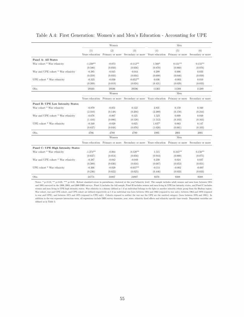
Table A.4: First Generation: Women’s and Men’s Education - Accounting for UPE

Women Men

(1) (2) (3) (4) (5) (6)

Years education Primary or more Secondary or more Years education Primary or more Secondary or more

Panel A: All States

War cohort * War ethnicity -1.239** -0.073 -0.112** 1.560* 0.131** 0.155**

(0.580) (0.050) (0.056) (0.870) (0.060) (0.076)

War and UPE cohort * War ethnicity -0.385 -0.045 -0.044 0.299 0.006 0.033

(0.359) (0.033) (0.034) (0.608) (0.046) (0.050)

UPE cohort * War ethnicity -0.323 -0.030 -0.052** 0.036 -0.003 0.010

(0.209) (0.019) (0.024) (0.421) (0.029) (0.033)

Obs. 29560 29596 29596 11365 11389 11389

Women Men

Years education Primary or more Secondary or more Years education Primary or more Secondary or more

Panel B: UPE Low Intensity States

War cohort * War ethnicity -0.879 -0.051 0.122 2.831 0.159 0.160

(2.310) (0.148) (0.204) (2.389) (0.158) (0.244)

War and UPE cohort * War ethnicity -0.676 -0.067 0.125 1.523 0.009 0.049

(1.416) (0.086) (0.128) (1.512) (0.102) (0.163)

UPE cohort * War ethnicity -0.340 -0.020 0.025 1.837* 0.063 0.147

(0.837) (0.048) (0.076) (1.020) (0.061) (0.103)

Obs. 4786 4789 4789 1995 2001 2001

Women Men

Years education Primary or more Secondary or more Years education Primary or more Secondary or more

Panel C: UPE High Intensity States

War cohort * War ethnicity -1.274** -0.064 -0.128** 1.515 0.165** 0.156**

(0.637) (0.054) (0.056) (0.944) (0.068) (0.075)

War and UPE cohort * War ethnicity -0.387 -0.042 -0.049 0.239 0.024 0.037

(0.389) (0.036) (0.034) (0.687) (0.053) (0.051)

UPE cohort * War ethnicity -0.366 -0.029 -0.057** -0.151 -0.002 -0.007

(0.236) (0.022) (0.025) (0.446) (0.033) (0.033)

Obs. 24774 24807 24807 9370 9388 9388

Notes: * p<0.10, ** p<0.05, *** p<0.01. Robust standard errors in parentheses, clustered at the year*ethnicity level. The sample includes adult women and men born between 1954

and 1981 surveyed in the 1999, 2003, and 2008 DHS surveys. Panel A includes the full sample, Panel B includes women and men living in UPE low intensity states, and Panel C includes

women and men living in UPE high intensity states. War ethnicity is a dummy defined as 1 if an individual belongs to the Igbo or another minority ethnic group from the Biafran region.

War cohort, war and UPE cohort, and UPE cohort are defined respectively as 1 if an individual was born between 1954 and 1963 (exposed to war only), between 1964 and 1970 (exposed

to war and UPE), and between 1971 and 1975 (exposed to UPE only). Cohorts exposed to neither the war nor the UPE are the omitted category (born between 1976 and 1981). In

addition to the war exposure interaction term, all regressions include DHS survey dummies, year, state, ethnicity fixed effects and ethnicity specific time trends. Dependent variables are

defined as in Table 3.

55

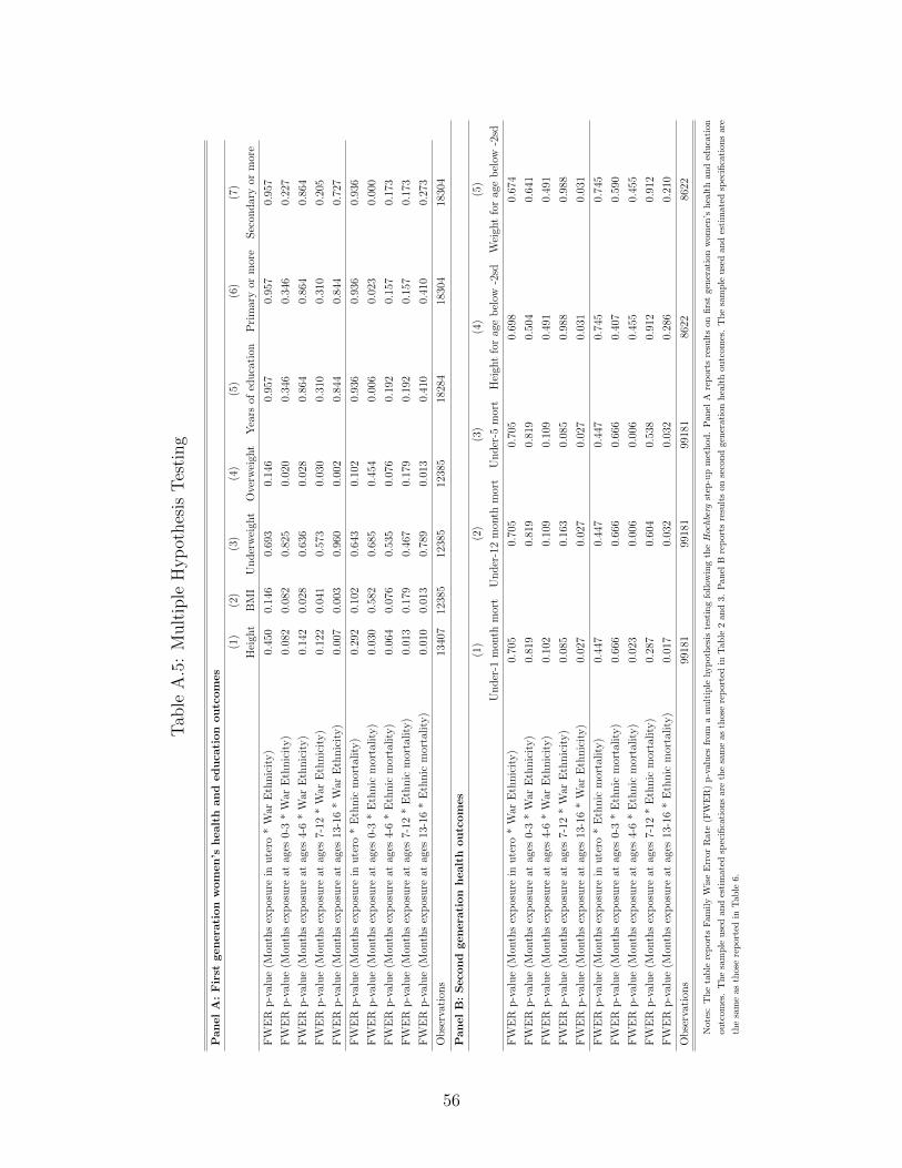
Tab

leA

.5:

Mult

iple

Hyp

othes

isT

esti

ng

Panel

A:

Fir

stgenera

tion

wom

en’s

healt

hand

educa

tion

outc

om

es

(1)

(2)

(3)

(4)

(5)

(6)

(7)

Hei

ght

BM

IU

nd

erw

eigh

tO

verw

eigh

tY

ears

ofed

uca

tion

Pri

mar

yor

mor

eS

econ

dar

yor

mor

e

FW

ER

p-v

alu

e(M

onth

sex

pos

ure

inu

tero

*W

arE

thn

icit

y)

0.45

00.

146

0.69

30.

146

0.95

70.

957

0.95

7

FW

ER

p-v

alu

e(M

onth

sex

pos

ure

atag

es0-

3*

War

Eth

nic

ity)

0.08

20.

082

0.82

50.

020

0.34

60.

346

0.22

7

FW

ER

p-v

alu

e(M

onth

sex

pos

ure

atag

es4-

6*

War

Eth

nic

ity)

0.14

20.

028

0.63

60.

028

0.86

40.

864

0.86

4

FW

ER

p-v

alu

e(M

onth

sex

pos

ure

atag

es7-

12*

War

Eth

nic

ity)

0.12

20.

041

0.57

30.

030

0.31

00.

310

0.20

5

FW

ER

p-v

alu

e(M

onth

sex

pos

ure

atag

es13

-16

*W

arE

thn

icit

y)

0.00

70.

003

0.96

00.

002

0.84

40.

844

0.72

7

FW

ER

p-v

alu

e(M

onth

sex

pos

ure

inu

tero

*E

thn

icm

orta

lity

)0.

292

0.10

20.

643

0.10

20.

936

0.93

60.

936

FW

ER

p-v

alu

e(M

onth

sex

pos

ure

atag

es0-

3*

Eth

nic

mor

tali

ty)

0.03

00.

582

0.68

50.

454

0.00

60.

023

0.00

0

FW

ER

p-v

alu

e(M

onth

sex

pos

ure

atag

es4-

6*

Eth

nic

mor

tali

ty)

0.06

40.

076

0.53

50.

076

0.19

20.

157

0.17

3

FW

ER

p-v

alu

e(M

onth

sex

pos

ure

atag

es7-

12*

Eth

nic

mor

tali

ty)

0.01

30.

179

0.46

70.

179

0.19

20.

157

0.17

3

FW

ER

p-v

alu

e(M

onth

sex

pos

ure

atag

es13

-16

*E

thn

icm

orta

lity

)0.

010

0.01

30.

789

0.01

30.

410

0.41

00.

273

Ob

serv

atio

ns

1340

712

385

1238

512

385

1828

418

304

1830

4

Panel

B:

Seco

nd

genera

tion

healt

houtc

om

es

(1)

(2)

(3)

(4)

(5)

Un

der

-1m

onth

mor

tU

nd

er-1

2m

onth

mor

tU

nd

er-5

mor

tH

eigh

tfo

rag

eb

elow

-2sd

Wei

ght

for

age

bel

ow-2

sd

FW

ER

p-v

alu

e(M

onth

sex

pos

ure

inu

tero

*W

arE

thn

icit

y)

0.70

50.

705

0.70

50.

698

0.67

4

FW

ER

p-v

alu

e(M

onth

sex

pos

ure

atag

es0-

3*

War

Eth

nic

ity)

0.81

90.

819

0.81

90.

504

0.64

1

FW

ER

p-v

alu

e(M

onth

sex

pos

ure

atag

es4-

6*

War

Eth

nic

ity)

0.10

20.

109

0.10

90.

491

0.49

1

FW

ER

p-v

alu

e(M

onth

sex

pos

ure

atag

es7-

12*

War

Eth

nic

ity)

0.08

50.

163

0.08

50.

988

0.98

8

FW

ER

p-v

alu

e(M

onth

sex

pos

ure

atag

es13

-16

*W

arE

thn

icit

y)

0.02

70.

027

0.02

70.

031

0.03

1

FW

ER

p-v

alu

e(M

onth

sex

pos

ure

inu

tero

*E

thn

icm

orta

lity

)0.

447

0.44

70.

447

0.74

50.

745

FW

ER

p-v

alu

e(M

onth

sex

pos

ure

atag

es0-

3*

Eth

nic

mor

tali

ty)

0.66

60.

666

0.66

60.

407

0.59

0

FW

ER

p-v

alu

e(M

onth

sex

pos

ure

atag

es4-

6*

Eth

nic

mor

tali

ty)

0.02

30.

006

0.00

60.

455

0.45

5

FW

ER

p-v

alu

e(M

onth

sex

pos

ure

atag

es7-

12*

Eth

nic

mor

tali

ty)

0.28

70.

604

0.53

80.

912

0.91

2

FW

ER

p-v

alu

e(M

onth

sex

pos

ure

atag

es13

-16

*E

thn

icm

orta

lity

)0.

017

0.03

20.

032

0.28

60.

210

Ob

serv

atio

ns

9918

199

181

9918

186

2286

22

Not

es:

The

table

rep

orts

Fam

ily

Wis

eE

rror

Rate

(FW

ER

)p-v

alu

esfr

oma

mult

iple

hyp

oth

esis

test

ing

follow

ing

theHochberg

step

-up

met

hod.

Pan

elA

rep

ort

sre

sult

son

firs

tgen

erati

on

wom

en’s

hea

lth

and

educa

tion

outc

omes

.T

he

sam

ple

use

dan

des

tim

ated

spec

ifica

tions

are

the

sam

eas

thos

ere

por

ted

inT

able

2an

d3.

Pan

elB

rep

orts

resu

lts

on

seco

nd

gener

atio

nhea

lth

outc

om

es.

The

sam

ple

use

dand

esti

mate

dsp

ecifi

cati

ons

are

the

sam

eas

thos

ere

por

ted

inT

able

6.

56

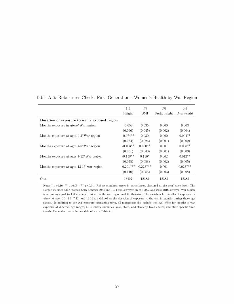
Table A.6: Robustness Check: First Generation - Women’s Health by War Region

(1) (2) (3) (4)

Height BMI Underweight Overweight

Duration of exposure to war x exposed region

Months exposure in utero*War region -0.059 0.035 0.000 0.003

(0.066) (0.045) (0.002) (0.004)

Months exposure at ages 0-3*War region -0.074** 0.030 0.000 0.004**

(0.034) (0.026) (0.001) (0.002)

Months exposure at ages 4-6*War region -0.103** 0.080** 0.001 0.008**

(0.051) (0.040) (0.001) (0.003)

Months exposure at ages 7-12*War region -0.158** 0.110* 0.002 0.012**

(0.075) (0.058) (0.002) (0.005)

Months exposure at ages 13-16*war region -0.291*** 0.228*** 0.001 0.023***

(0.110) (0.085) (0.003) (0.008)

Obs. 13407 12385 12385 12385

Notes:* p<0.10, ** p<0.05, *** p<0.01. Robust standard errors in parentheses, clustered at the year*state level. The

sample includes adult women born between 1954 and 1974 and surveyed in the 2003 and 2008 DHS surveys. War region

is a dummy equal to 1 if a woman resided in the war region and 0 otherwise. The variables for months of exposure in

utero, at ages 0-3, 4-6, 7-12, and 13-16 are defined as the duration of exposure to the war in months during those age

ranges. In addition to the war exposure interaction term, all regressions also include the level effect for months of war

exposure at different age ranges, DHS survey dummies, year, state, and ethnicity fixed effects, and state specific time

trends. Dependent variables are defined as in Table 2.

57

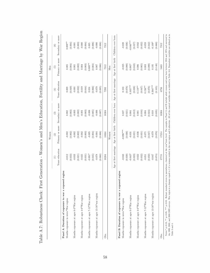
Tab

leA

.7:

Rob

ust

nes

sC

hec

k:

Fir

stG

ener

atio

n-

Wom

en’s

and

Men

’sE

duca

tion

,F

erti

lity

and

Mar

riag

eby

War

Reg

ion

Wom

enM

en

(1)

(2)

(3)

(4)

(5)

(6)

Yea

rsed

uca

tion

Pri

mar

yor

mor

eS

econ

dar

yor

mor

eY

ears

edu

cati

onP

rim

ary

orm

ore

Sec

ond

ary

orm

ore

Pan

el

A:

Du

rati

on

of

exp

osu

reto

war

xexp

ose

dre

gio

n

Mon

ths

exp

osu

rein

ute

ro*W

arre

gion

-0.0

12-0

.002

0.00

20.

009

0.00

50.

009*

*

(0.0

33)

(0.0

02)

(0.0

03)

(0.0

49)

(0.0

04)

(0.0

04)

Mon

ths

exp

osu

reat

ages

0-3*

War

regi

on-0

.033

-0.0

02-0

.003

-0.0

010.

001

-0.0

01

(0.0

21)

(0.0

02)

(0.0

02)

(0.0

32)

(0.0

02)

(0.0

03)

Mon

ths

exp

osu

reat

ages

4-6*

War

regi

on-0

.025

-0.0

02-0

.001

-0.0

190.

004

-0.0

00

(0.0

31)

(0.0

03)

(0.0

03)

(0.0

44)

(0.0

03)

(0.0

04)

Mon

ths

exp

osu

reat

ages

7-12

*War

regi

on-0

.081

*-0

.005

-0.0

060.

034

0.00

9**

0.00

5

(0.0

45)

(0.0

04)

(0.0

05)

(0.0

66)

(0.0

04)

(0.0

06)

Mon

ths

exp

osu

reat

ages

13-1

6*w

arre

gion

-0.0

78-0

.004

-0.0

06-0

.070

0.00

7-0

.000

(0.0

68)

(0.0

06)

(0.0

07)

(0.0

95)

(0.0

06)

(0.0

08)

Ob

s.18

284

1830

418

304

7292

7312

7312

Wom

enM

en

Age

atfi

rst

mar

riag

eA

geat

firs

tb

irth

Ch

ild

ren

ever

bor

nA

geat

firs

tm

arri

age

Age

atfi

rst

bir

thC

hil

dre

nev

erb

orn

Pan

el

B:

Du

rati

on

of

exp

osu

reto

war

xexp

ose

dre

gio

n

Mon

ths

exp

osu

rein

ute

ro*W

arre

gion

-0.0

43-0

.096

***

0.02

70.

103

-0.0

25-0

.039

(0.0

39)

(0.0

36)

(0.0

21)

(0.0

76)

(0.0

80)

(0.0

36)

Mon

ths

exp

osu

reat

ages

0-3*

War

regi

on-0

.043

*-0

.031

0.00

40.

105*

**0.

085*

-0.0

46**

*

(0.0

23)

(0.0

21)

(0.0

12)

(0.0

38)

(0.0

43)

(0.0

17)

Mon

ths

exp

osu

reat

ages

4-6*

War

regi

on-0

.022

-0.0

360.

001

0.11

9**

0.08

6-0

.042

(0.0

32)

(0.0

31)

(0.0

16)

(0.0

47)

(0.0

65)

(0.0

32)

Mon

ths

exp

osu

reat

ages

7-12

*War

regi

on-0

.051

-0.0

710.

004

0.15

6**

0.08

3-0

.059

(0.0

50)

(0.0

47)

(0.0

24)

(0.0

76)

(0.0

99)

(0.0

42)

Mon

ths

exp

osu

reat

ages

13-1

6*w

arre

gion

-0.0

47-0

.079

0.01

80.

304*

**0.

195

-0.1

09*

(0.0

74)

(0.0

70)

(0.0

35)

(0.1

05)

(0.1

48)

(0.0

60)

Ob

s.17

715

1721

418

304

6756

5463

7312

Not

es:*

p<

0.10

,**

p<

0.05

,**

*p<

0.0

1.R

ob

ust

stan

dar

der

rors

inp

aren

thes

es,

clu

ster

edat

the

year

*sta

tele

vel.

Th

esa

mp

les

inP

anel

Aan

dB

incl

ud

ead

ult

wom

enan

dm

enb

orn

bet

wee

n195

4an

d19

74an

dsu

rvey

edin

the

1999

,20

03,

and

2008

DH

Ssu

rvey

s.W

arre

gion

isa

du

mm

yeq

ual

to1

ifa

wom

an

resi

ded

inth

ew

ar

regio

nan

d0

oth

erw

ise.

All

of

the

contr

olva

riab

les

are

asd

efin

edin

Tab

leA

.6.

Dep

end

ent

vari

ab

les

are

defi

ned

asin

Tab

le3

and

4.

58

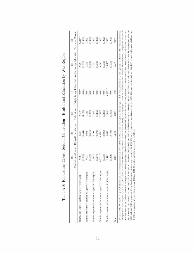
Tab

leA

.8:

Rob

ust

nes

sC

hec

k:

Sec

ond

Gen

erat

ion

-H

ealt

han

dE

duca

tion

by

War

Reg

ion

(1)

(2)

(3)

(4)

(5)

(6)

Un

der

-1m

onth

mor

tU

nd

er-1

2m

onth

sm

ort

Und

er-5

mor

tH

eigh

tfo

rag

eb

elow

-2sd

Wei

ght

for

age

bel

ow-2

sdE

du

cati

onZ

scor

e

Mon

ths

exp

osu

reof

mot

her

inu

tero

*War

regi

on-0

.497

-0.7

54-0

.340

0.00

0-0

.004

-0.0

15**

(0.5

32)

(1.0

04)

(1.1

52)

(0.0

04)

(0.0

03)

(0.0

06)

Mon

ths

exp

osu

reof

mot

her

atag

es0-

3*W

arre

gion

-0.0

130.

084

0.18

60.

001

0.00

10.

002

(0.1

95)

(0.3

16)

(0.3

96)

(0.0

01)

(0.0

01)

(0.0

02)

Mon

ths

exp

osu

reof

mot

her

atag

es4-

6*W

arre

gion

0.43

0**

0.39

80.

364

0.00

10.

000

0.00

0

(0.2

05)

(0.3

73)

(0.4

62)

(0.0

01)

(0.0

01)

(0.0

02)

Mon

ths

exp

osu

reof

mot

her

atag

es7-

12*W

arre

gion

0.51

2***

0.47

9*0.

782*

*0.

002

-0.0

010.

000

(0.1

94)

(0.2

89)

(0.3

33)

(0.0

01)

(0.0

01)

(0.0

02)

Mon

ths

exp

osu

reof

mot

her

atag

es13

-16*

war

regi

on0.

418

0.64

31.

163*

0.00

7**

0.01

1**

0.00

3

(0.3

98)

(0.5

38)

(0.6

67)

(0.0

03)

(0.0

05)

(0.0

04)

Ob

s.99

181

9918

199

181

8622

8622

2620

9

Not

es:*

p<

0.10

,**

p<

0.0

5,**

*p<

0.0

1.R

obu

stst

andard

erro

rsin

pare

nth

eses

,cl

ust

ered

at

the

year*

state

leve

l.W

arre

gio

nis

ad

um

my

equ

al

to1

ifa

wom

an

resi

ded

inth

ew

ar

regi

onan

d0

oth

erw

ise.

Th

eva

riab

les

for

mon

ths

ofex

pos

ure

inutero

,at

ages

0-3,

4-6,

7-12

,an

d13

-16

are

defi

ned

as

the

du

rati

on

of

exp

osu

reto

the

war

inm

onth

sd

uri

ng

thos

eage

ran

ges.

Inad

dit

ion

toth

em

oth

er’s

war

exp

osu

rein

tera

ctio

nte

rm,

all

regre

ssio

ns

also

incl

ud

e

the

level

effec

tfo

rth

em

oth

er’s

mon

ths

ofw

arex

posu

reat

diff

eren

tage

ran

ges

,D

HS

surv

eyd

um

mie

s,yea

r(m

oth

eran

dch

ild

),st

ate

,an

det

hn

icit

yfi

xed

effec

ts,

and

stat

esp

ecifi

cti

me

tren

ds,

ad

um

my

for

wh

eth

erth

ech

ild

isa

girl

.C

olu

mn

s1

to3

use

the

1999

,20

03,

and

2008

DH

Ssu

rvey

san

din

clu

de

all

chil

dre

nb

orn

aft

er197

0to

mot

her

sw

ho

wer

eb

orn

bet

wee

n19

54

and

197

4.

Colu

mn

s4

and

5in

clud

ech

ild

ren

born

inth

efi

ve

year

sp

rece

din

gth

e

2003

and

2008

DH

Ssu

rvey

s(a

nd

du

eto

data

lim

itat

ion

sth

eth

ree

years

pre

ced

ing

the

1999

DH

Ssu

rvey

)to

mot

her

sb

orn

bet

wee

n19

54an

d19

74.

Col

um

n6

use

sth

e200

3and

2008

DH

Ssu

rvey

san

din

clu

des

all

chil

dre

nage

6-18

bor

nto

mot

her

sw

ho

wer

eb

orn

bet

wee

n19

54

an

d1974

.D

epen

den

tva

riab

les

are

defi

ned

asin

Tab

le6.

59

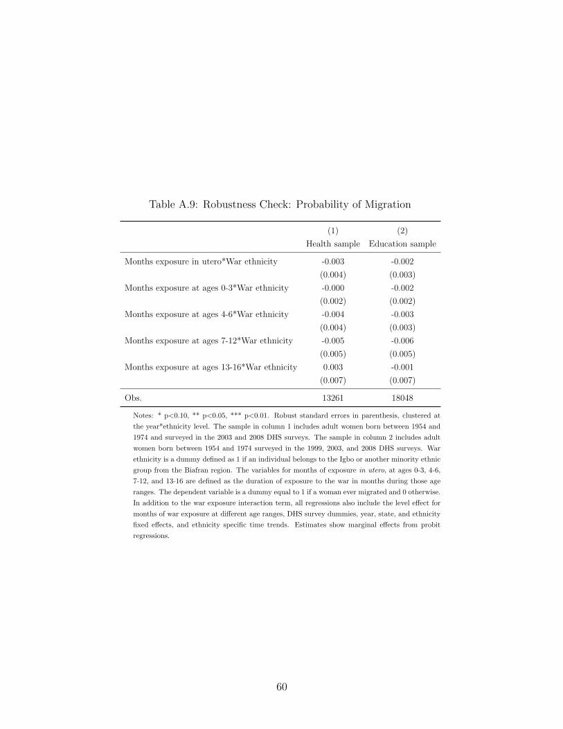
Table A.9: Robustness Check: Probability of Migration

(1) (2)

Health sample Education sample

Months exposure in utero*War ethnicity -0.003 -0.002

(0.004) (0.003)

Months exposure at ages 0-3*War ethnicity -0.000 -0.002

(0.002) (0.002)

Months exposure at ages 4-6*War ethnicity -0.004 -0.003

(0.004) (0.003)

Months exposure at ages 7-12*War ethnicity -0.005 -0.006

(0.005) (0.005)

Months exposure at ages 13-16*War ethnicity 0.003 -0.001

(0.007) (0.007)

Obs. 13261 18048

Notes: * p<0.10, ** p<0.05, *** p<0.01. Robust standard errors in parenthesis, clustered at

the year*ethnicity level. The sample in column 1 includes adult women born between 1954 and

1974 and surveyed in the 2003 and 2008 DHS surveys. The sample in column 2 includes adult

women born between 1954 and 1974 surveyed in the 1999, 2003, and 2008 DHS surveys. War

ethnicity is a dummy defined as 1 if an individual belongs to the Igbo or another minority ethnic

group from the Biafran region. The variables for months of exposure in utero, at ages 0-3, 4-6,

7-12, and 13-16 are defined as the duration of exposure to the war in months during those age

ranges. The dependent variable is a dummy equal to 1 if a woman ever migrated and 0 otherwise.

In addition to the war exposure interaction term, all regressions also include the level effect for

months of war exposure at different age ranges, DHS survey dummies, year, state, and ethnicity

fixed effects, and ethnicity specific time trends. Estimates show marginal effects from probit

regressions.

60

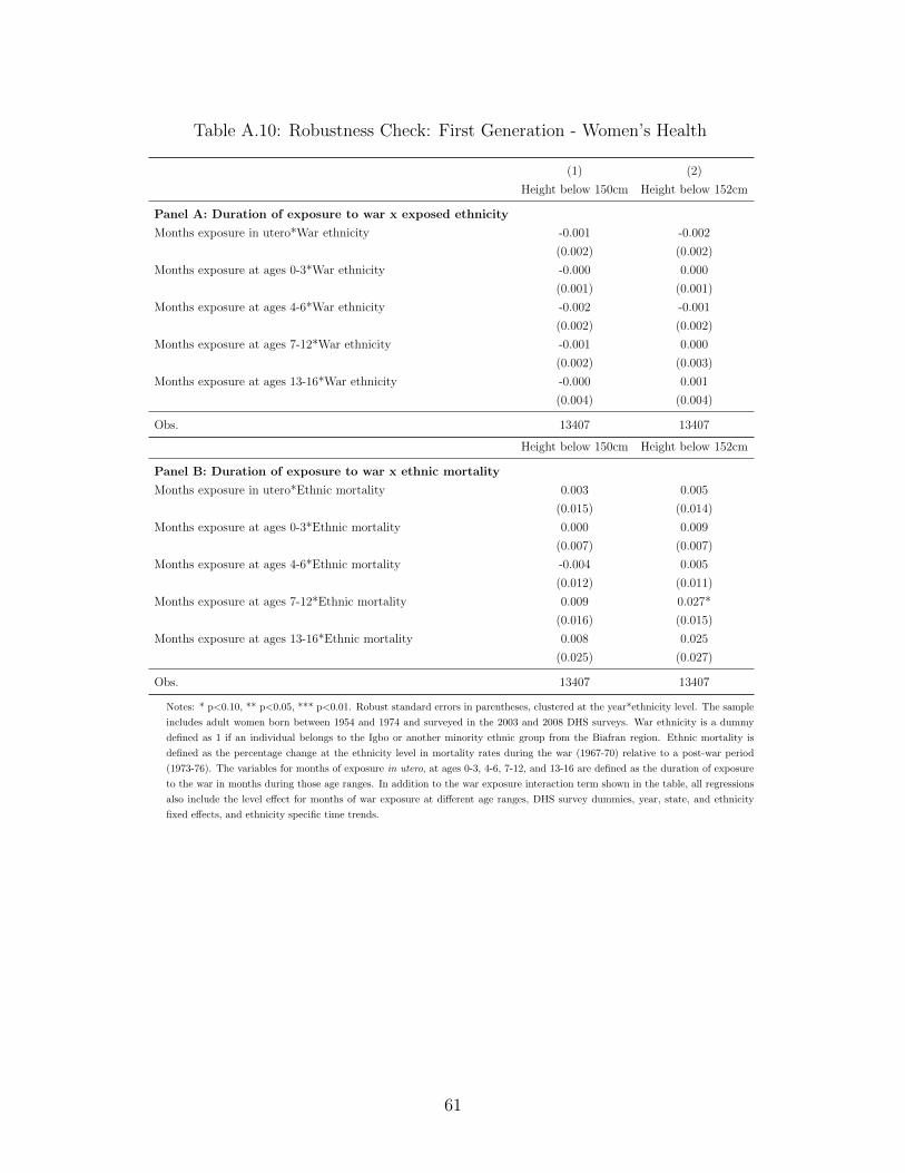
Table A.10: Robustness Check: First Generation - Women’s Health

(1) (2)

Height below 150cm Height below 152cm

Panel A: Duration of exposure to war x exposed ethnicity

Months exposure in utero*War ethnicity -0.001 -0.002

(0.002) (0.002)

Months exposure at ages 0-3*War ethnicity -0.000 0.000

(0.001) (0.001)

Months exposure at ages 4-6*War ethnicity -0.002 -0.001

(0.002) (0.002)

Months exposure at ages 7-12*War ethnicity -0.001 0.000

(0.002) (0.003)

Months exposure at ages 13-16*War ethnicity -0.000 0.001

(0.004) (0.004)

Obs. 13407 13407

Height below 150cm Height below 152cm

Panel B: Duration of exposure to war x ethnic mortality

Months exposure in utero*Ethnic mortality 0.003 0.005

(0.015) (0.014)

Months exposure at ages 0-3*Ethnic mortality 0.000 0.009

(0.007) (0.007)

Months exposure at ages 4-6*Ethnic mortality -0.004 0.005

(0.012) (0.011)

Months exposure at ages 7-12*Ethnic mortality 0.009 0.027*

(0.016) (0.015)

Months exposure at ages 13-16*Ethnic mortality 0.008 0.025

(0.025) (0.027)

Obs. 13407 13407

Notes: * p<0.10, ** p<0.05, *** p<0.01. Robust standard errors in parentheses, clustered at the year*ethnicity level. The sample

includes adult women born between 1954 and 1974 and surveyed in the 2003 and 2008 DHS surveys. War ethnicity is a dummy

defined as 1 if an individual belongs to the Igbo or another minority ethnic group from the Biafran region. Ethnic mortality is

defined as the percentage change at the ethnicity level in mortality rates during the war (1967-70) relative to a post-war period

(1973-76). The variables for months of exposure in utero, at ages 0-3, 4-6, 7-12, and 13-16 are defined as the duration of exposure

to the war in months during those age ranges. In addition to the war exposure interaction term shown in the table, all regressions

also include the level effect for months of war exposure at different age ranges, DHS survey dummies, year, state, and ethnicity

fixed effects, and ethnicity specific time trends.

61

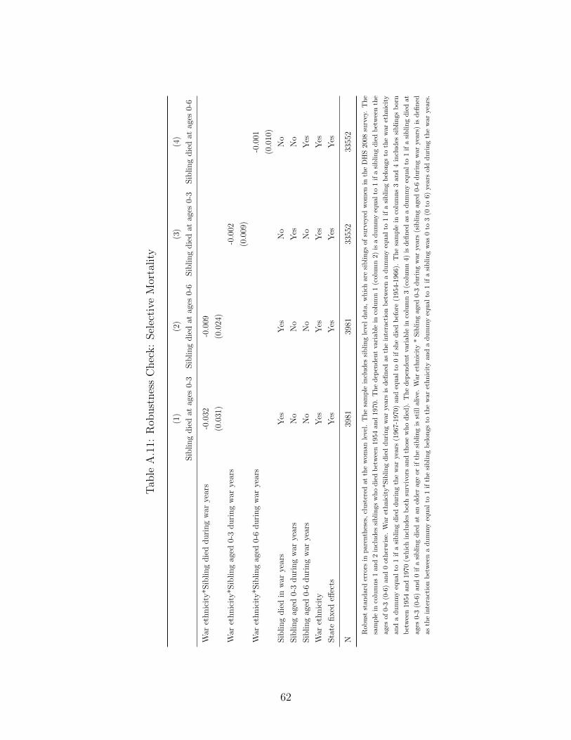
Tab

leA

.11:

Rob

ust

nes

sC

hec

k:

Sel

ecti

veM

orta

lity

(1)

(2)

(3)

(4)

Sib

ling

die

dat

ages

0-3

Sib

ling

die

dat

ages

0-6

Sib

ling

die

dat

ages

0-3

Sib

ling

die

dat

ages

0-6

War

ethnic

ity*S

ibling

die

dduri

ng

war

year

s-0

.032

-0.0

09

(0.0

31)

(0.0

24)

War

ethnic

ity*S

ibling

aged

0-3

duri

ng

war

year

s-0

.002

(0.0

09)

War

ethnic

ity*S

ibling

aged

0-6

duri

ng

war

year

s-0

.001

(0.0

10)

Sib

ling

die

din

war

year

sY

esY

esN

oN

o

Sib

ling

aged

0-3

duri

ng

war

year

sN

oN

oY

esN

o

Sib

ling

aged

0-6

duri

ng

war

year

sN

oN

oN

oY

es

War

ethnic

ity

Yes

Yes

Yes

Yes

Sta

tefixed

effec

tsY

esY

esY

esY

es

N39

8139

8133

552

3355

2

Rob

ust

stan

dar

der

rors

inp

are

nth

eses

,cl

ust

ered

atth

ew

om

an

leve

l.T

he

sam

ple

incl

ud

essi

bli

ng

leve

ld

ata

,w

hic

har

esi

bli

ngs

ofsu

rvey

edw

omen

inth

eD

HS

2008

surv

ey.

Th

e

sam

ple

inco

lum

ns

1an

d2

incl

ud

essi

bli

ngs

who

die

db

etw

een

195

4an

d197

0.T

he

dep

end

ent

vari

ab

lein

colu

mn

1(c

olu

mn

2)is

ad

um

my

equ

alto

1if

asi

bli

ng

die

db

etw

een

the

ages

of0-

3(0

-6)

and

0ot

her

wis

e.W

ar

eth

nic

ity*S

ibli

ng

die

dd

uri

ng

war

year

sis

defi

ned

as

the

inte

ract

ion

bet

wee

na

dum

my

equ

al

to1

ifa

sib

lin

gb

elon

gsto

the

war

eth

nic

ity

and

ad

um

my

equ

al

to1

ifa

sib

lin

gd

ied

du

rin

gth

ew

ar

years

(1967-1

970)

an

deq

ual

to0

ifsh

ed

ied

bef

ore

(1954

-196

6).

Th

esa

mp

lein

colu

mn

s3

and

4in

clu

des

sib

lin

gs

born

bet

wee

n195

4an

d19

70

(wh

ich

incl

ud

esb

oth

surv

ivors

and

thos

ew

ho

die

d).

Th

ed

epen

den

tva

riab

lein

colu

mn

3(c

olu

mn

4)is

defi

ned

asa

du

mm

yeq

ual

to1

ifa

sib

lin

gd

ied

at

ages

0-3

(0-6

)and

0if

asi

bli

ng

die

dat

anold

erag

eor

ifth

esi

bli

ng

isst

ill

ali

ve.

War

eth

nic

ity

*S

ibli

ng

age

d0-3

du

rin

gw

aryea

rs(s

ibli

ng

aged

0-6

du

rin

gw

aryea

rs)

isd

efin

ed

asth

ein

tera

ctio

nb

etw

een

ad

um

my

equal

to1

ifth

esi

bli

ng

bel

on

gs

toth

ew

ar

eth

nic

ity

and

ad

um

my

equ

al

to1

ifa

sib

lin

gw

as0

to3

(0to

6)ye

ars

old

du

rin

gth

ew

arye

ars.

62

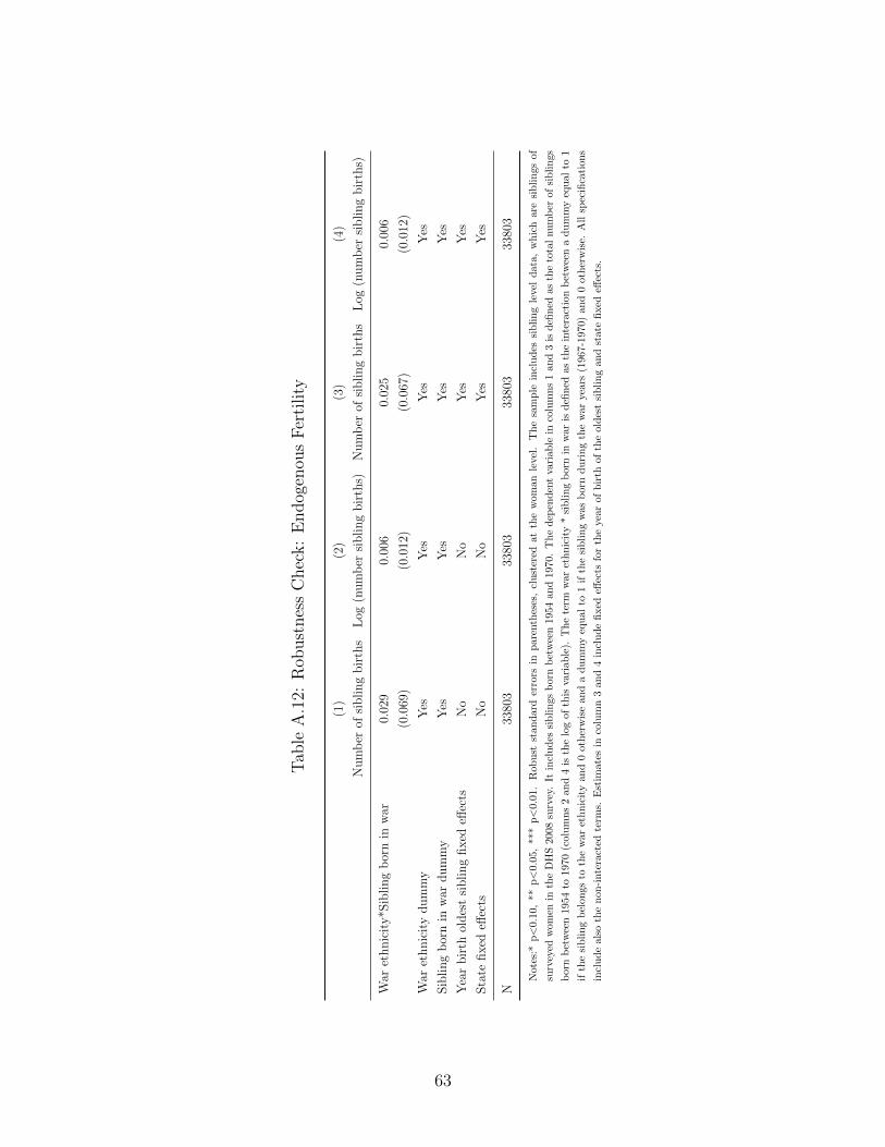
Tab

leA

.12:

Rob

ust

nes

sC

hec

k:

Endog

enou

sF

erti

lity

(1)

(2)

(3)

(4)

Num

ber

ofsi

bling

bir

ths

Log

(num

ber

sibling

bir

ths)

Num

ber

ofsi

bling

bir

ths

Log

(num

ber

sibling

bir

ths)

War

ethnic

ity*S

ibling

bor

nin

war

0.02

90.

006

0.02

50.

006

(0.0

69)

(0.0

12)

(0.0

67)

(0.0

12)

War

ethnic

ity

dum

my

Yes

Yes

Yes

Yes

Sib

ling

bor

nin

war

dum

my

Yes

Yes

Yes

Yes

Yea

rbir

thol

des

tsi

bling

fixed

effec

tsN

oN

oY

esY

es

Sta

tefixed

effec

tsN

oN

oY

esY

es

N33

803

3380

333

803

3380

3

Not

es:*

p<

0.10

,**

p<

0.0

5,

***

p<

0.01.

Rob

ust

stand

ard

erro

rsin

pare

nth

eses

,cl

ust

ered

atth

ew

om

anle

vel.

Th

esa

mp

lein

clu

des

sib

lin

gle

vel

dat

a,

wh

ich

are

sib

lin

gsof

surv

eyed

wom

enin

the

DH

S20

08su

rvey

.It

incl

ud

essi

bli

ngs

bor

nb

etw

een

195

4an

d197

0.T

he

dep

end

ent

vari

ab

lein

colu

mn

s1

and

3is

defi

ned

asth

eto

tal

nu

mb

erof

sib

lin

gs

bor

nb

etw

een

1954

to19

70

(col

um

ns

2an

d4

isth

elo

gof

this

vari

able

).T

he

term

war

eth

nic

ity

*si

bli

ng

bor

nin

war

isd

efin

edas

the

inte

ract

ion

bet

wee

na

du

mm

yeq

ual

to1

ifth

esi

bli

ng

bel

ongs

toth

ew

aret

hn

icit

yan

d0

oth

erw

ise

an

da

du

mm

yeq

ual

to1

ifth

esi

bli

ng

was

born

du

rin

gth

ew

ar

year

s(1

967-

197

0)

an

d0

oth

erw

ise.

All

spec

ifica

tion

s

incl

ud

eal

soth

en

on-i

nte

ract

edte

rms.

Est

imate

sin

colu

mn

3an

d4

incl

ud

efi

xed

effec

tsfo

rth

eye

ar

ofb

irth

ofth

eol

des

tsi

bli

ng

an

dst

ate

fixed

effec

ts.

63

B Data appendix

B.1 Data and samples

DHS survey sample

In the DHS 2008 survey, all women age 15-49 who were either permanent residents of the

households in the DHS survey sample or visitors present in the households on the night

before the survey were eligible to be interviewed. In a sub-sample of half of the households,

all men age 15-59 who were either permanent residents of the households in the 2008 sample

or visitors present in the households on the night before the survey were eligible to be

interviewed (NPC, 2009). Similarly, in the DHS 2003 (DHS 1999) survey, a probability

sample of households was selected and all women age 15-49 (10-49 in the DHS 1999 survey)

identified in the household were eligible to be interviewed. In a sub-sample of one-third of

the households selected for the survey, all men 15-59 (15-64 in the DHS 1999 survey) were

eligible to be interviewed (NPC, 2000, 2004).

First generation sample

Health outcomes : For the first generation analysis on health outcomes we use the sample

of women in the 2003 and 2008 DHS as health indicators are only collected for the sample

of women. We do not use the DHS 1999 survey for the analysis of first generation health

outcomes because the nutritional status and height of women is collected only for women who

had a birth in the 3 years prior to the survey year, which would result in a non-representative

sub-sample of interviewed women. The DHS 2003 includes women born since 1954 and the

DHS 2008 those born since 1958. We choose the 1974 birth cohort as the upper bound in

our sample in order to reduce possible confounding effects. Moreover, we need to include

adult individuals that have completed their growth process.

Education, fertility, and marriage outcomes : For the analysis of education, fertility, and

marriage outcomes, we use the sample of women and men in the three DHS surveys from

1999, 2003, and 2008. We include both women and men born between 1954 (1958 for the

2008 DHS survey) and 1974. As for the health outcomes we choose the 1974 birth cohort as

the upper bound in our sample in order to reduce possible confounding effects. Moreover,

we need to include adult individuals that have completed their education processes.

Second generation sample

We use the information on the fertility histories of mothers in the three DHS surveys from

1999, 2003, and 2008 to construct a child level sample for the analysis of second generation

64

children. The 1999 DHS survey, while not containing information on health outcomes of all

women, includes information on the year of birth and the state of residence of all women

15-49 years old. This additional dataset allows including mothers and children born in earlier

years and hence covering additional cohorts. The sample we use for the second generation

analysis includes all children born to mothers who had at least one child. The child-level

sample is based on children of mothers born between 1954 and 1974 (i.e., this is consistent

with the sample used for the first generation analysis). We further restrict the sample to

children born after 1970 to avoid any confounding effect of the war on second generation

children.

There is a likelihood of under-reporting of births and deaths of children not alive at the

time of the survey because the mother may be reluctant to talk about deceased children.

Children’ deaths in early infancy may be those most likely under reported. However, as

the proportion of neonatal deaths in our surveys is substantial, this may suggest that the

under-reporting is not severe (NPC, 2000, 2004, 2009).

Second generation sample for education outcome

Children’s educational attainment can be only retrieved in the 2003 and 2008 DHS surveys.

The 1999 DHS survey does not contain the identifier that allows one to match the household

level dataset (which contain information on education) with the child level dataset that we

use for the analysis. Only children that are listed in the household level dataset and that are

alive can be matched to the child level dataset. We further restrict the sample to children

that are aged 6-18 at the time of the survey to account for potential selection of children

that stay or leave home once they turn 18.

Couple sample

The couple sample is obtained by matching each woman in the women’s sample to her

husband in the male sample. We are only able to match men and women that live in the

same household and that are currently married. The size of the couple sample is smaller

than the full sample because, as explained above, men were only surveyed in a sub-sample of

half of the households included in the women’s sample. Men can have polygamous unions.

We include all women that could be married to the same man.

For the second generation outcomes, we match women to their children, hence restricting

the sample to women that had at least one child. For consistency with our main analysis

we further restrict the sample to women that were born between 1954 and 1974. The father

sample is further restricted to only men that were born between 1954 and 1974.

65

B.2 Variables definitions

BMI, underweight, and overweight : We look at BMI as a continuous measure and at over-

weight and underweight indicators. Pregnant women at the time of the survey are excluded

from this sample. The underweight variable is a dummy defined as equal to 1 if the BMI of

an adult woman is below 18.5 and 0 otherwise. The overweight indicator is defined as equal

to 1 if the BMI is above 25 and 0 otherwise.

Education: We look at the years of completed education and at primary and secondary

school completion. Primary school completion is a dummy defined as 1 if an individual has

completed at least primary school and 0 otherwise. Similarly, secondary school completion

is a dummy defined as 1 if an individual has completed at least secondary school and 0

otherwise. We use information on women and men. We choose for both women and men

the same sample used for the health outcomes.

Ethnic mortality exposure: The information on siblings is reported only in the 1999 and

2008 DHS surveys but not in the 2003 DHS survey. In the 2008 survey, each woman was

asked to report information on her siblings and their related date of birth and death. We

use these data to construct mortality rates of siblings at different time periods. The sibling

mortality rate at the ethnicity level during the war is calculated as the ratio of the number of

siblings who died during the war (1967-70) and the total number of siblings born before 1970.

Similarly, the mortality rate after the war is calculated as the ratio of the number of siblings

who died after the war between 1973 and 1976 and the number of siblings born before 1976.

We obtain a measure of ethnic mortality as the percentage change in siblings’ mortality rates

between the war years and post-war years as follows: ethnic mortalitye=(mortality rate in

ware - mortality rate after ware) / mortality rate after ware.

Child mortality : We construct binary variables equal to 1 x 1000 if the child died within 1

month, 12 months, and five years after birth and 0 if the child is still alive or died afterwards.

Since this sample includes children born between 1966 and 2008, we restrict the sample to

children born after 1970 to avoid including confounding effects from the war years.

Height-for-age Z-score: This nutritional status indicator is expressed in standard devia-

tion (SD) units from the median of the reference population as calculated in the NDHS/CDC/

WHO Child Growth Standards (NPC, 2000, 2004, 2009). We define the height-for-age indi-

cator as a binary variable equal to 1 if the height-for-age Z-score is below minus 2 standard

deviations from the reference population median. Children below this threshold are con-

sidered stunted and so chronically malnourished. We define the weight-for-age indicator as

a binary variable equal to 1 if the weight-for-age Z-score is below minus 2 standard devia-

tions from the reference population median. Children below this threshold are considered

underweight. Anthropometric data on height are only collected on children born in the five

66

years prior to the 2008 and 2003 DHS surveys and in the three years prior to the 1999 DHS

survey. Therefore, the sample includes children born between 1996 and 2008 from mothers

born between 1954 and 1974.

Education Z-score: The outcome we analyze is the education Z-score that is calculated

as the deviation of a child’s completed years of education from the mean years of education

and divided by its standard deviation calculated on a sample of children aged 6-18 years old.

The average and standard deviation of the completed years of education are calculated at

the DHS survey year, child age, and state level. The sample includes only children that are

aged 6-18 years old.

67