finn haugen: pid control -...

Finn Haugen: PID Control 253

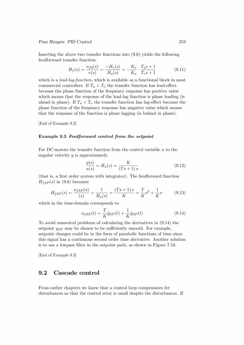
Inserting the above two transfer functions into (9.6) yields the followingfeedforward transfer function:

Hf (s) =ufd(s)

v(s)=−Hv(s)Hu(s)

= −KvKu

· Tus+ 1Tvs+ 1

(9.11)

which is a lead-lag-function, which is available as a functional block in mostcommercial controllers. If Tu > Tv the transfer function has lead-effectbecause the phase function of the frequency response has positive valuewhich means that the response of the lead-lag function is phase leading (isahead in phase). If Tu < Tv the transfer function has lag-effect because thephase function of the frequency response has negative value which meansthat the response of the function is phase lagging (is behind in phase).

[End of Example 9.2]

Example 9.3 Feedforward control from the setpoint

For DC-motors the transfer function from the control variable u to theangular velocity y is approximately

y(s)

u(s)= Hu(s) =

K

(Ts+ 1) s(9.12)

(that is, a first order system with integrator). The feedforward functionHfSP (s) in (9.6) becomes

HfSP (s) =ufSP (s)

(s)=

1

Hu(s)=(Ts+ 1) s

K=T

Ks2 +

1

Ks (9.13)

which in the time-domain corresponds to

ufSP (t) =T

KySP (t) +

1

KySP (t) (9.14)

To avoid numerical problems of calculating the derivatives in (9.14) thesetpoint ySP may be chosen to be sufficiently smooth. For example,setpoint changes could be in the form of parabolic functions of time sincethis signal has a continuous second order time derivative. Another solutionis to use a lowpass filter in the setpoint path, as shown in Figure 7.18.


9.2 Cascade control

From earlier chapters we know that a control loop compensates fordisturbances so that the control error is small despite the disturbances. If

254 Finn Haugen: PID Control

the controller has integral action the steady-state control error is zero.What more can we wish? In some applications it may be desirable if thetransient time progression of the error is faster, so that e.g. the IAE index,cf. Section 2.8, is smaller. This can be achieved by cascade control , seeFigure 9.7.

In a cascade control system there is one or more control loops inside theprimary loop, and the controllers are in cascade. There is usually one, but

Mr C1 C2 P2 P1

M2

M1

u y

v

ymSP eySP u1

Scaling

ym

y2

Sensors with scalings

DisturbancePrimary

controllerSecondarycontroller

Primary loop

Secondary loop

Secondaryoutput

Primaryoutput

Process

Figure 9.7: Cascade control system

there may be two and even three internal loops inside the primary loop.The (first) loop inside the primary loop is called the secondary loop, andthe controller in this loop is called the secondary controller (or slavecontroller). The outer loop is called the primary loop, and the controller inthis loop is called the primary controller (or master-controller). Thecontrol signal calculated by the primary controller is the setpoint of thesecondary controller.

In most applications the purpose of the secondary loop is to compensatequickly for the disturbance so that its response in the primary outputvariable of the process is small. For this to happen the secondary loop mustregister the disturbance. This is done with the sensor M2 in Figure 9.7.

In addition to getting better disturbance compensation cascade controlmay give a more linear relation between the variables u1 and y2, see Figure9.7 than with usual single loop control. In many applications process part2 (P2 in Figure 9.7) is the actuator. In this case the secondary loop can beregarded as a new actuator having better linearity (or proportionality).One example is a control valve where the secondary loop is a flow controlloop. With this secondary loop there is a more linear relation between the


control signal and the flow than without such a loop. The better linearitymay make the tuning of the primary controller (performing e.g. level ortemperature control) easier and with more robust stability properties.

The improved control with cascade control can be explained by theincreased information about the process — there is at least one moremeasurement. It is a general principle that the more information you haveabout the process to be controlled, the better it can be controlled. Notehowever, that there is still only one control variable to the process, but itis based on two or more measurements.

Since cascade control requires at least two sensors a cascade control systemis somewhat more expensive than a single loop control system. Except forcheap control equipment, commercial control equipment are typicallyprepared for cascade control, so no extra control hardware or software isrequired.

In which frequency range is the secondary loop effective for compensationfor disturbances? This is given by the bandwidth of the secondary loop. Aproper bandwidth definition here is the −11 dB-the bandwidth ωs of thesensitivity function, S2(s), of the secondary loop, cf. Chapter 6.3.4. S2(s)is

S2(s) =1

1 + L2(s)=

1

1 +Hc2(s)Hu2(s)Hm2(s)(9.15)

where L2(s) is the loop transfer function of the secondary loop. Hc2(s) isthe transfer function of the secondary controller. Hu2(s) is the transferfunction from the control variable to the secondary process output variable,y2. Hm2(s) is the measurement transfer function of the secondary sensor.

As explained above cascade control can give substantial compensationimprovement. Cascade control can also give improved tracking of a varyingsetpoint, but only if the secondary loop has faster dynamics than theprocess part P2 itself, cf. Figure 9.7, so that the primary controller “sees”a faster process. If there is a time delay in P2, the secondary loop will notbe faster than P2 (this is demonstrated in Example 9.4). In mostapplications improved compensation — not improved tracking — is the mainpurpose of cascade control.

The secondary controller is typically a P controller or a PI controller. Thederivative action is usually not needed to speed up the secondary loopsince process part 2 anyway has faster dynamics than process part 1, sothe secondary loop becomes fast enough. And in general the noise sensitivederivative term is a drawback. The primary controller is typically a PIDcontroller or a PI controller.


In the secondary controller the P- and the D-term should not have reducedsetpoint weights, cf. Section 2.7.1. Why?2

How do you tune the controllers of a cascade control? You can follow thisprocedure:

• First the secondary controller is tuned, with the primary controller inmanual mode.

• Then the primary controller is tuned, the secondary controller inautomatic mode.

Controller tuning can be made using a standard tuning method, e.g. theZiegler-Nichols’ closed loop method, cf. Section 4.4.

Example 9.4 Cascade control (simulation)

In this example the following two control systems are simulatedsimultaneously (in parallel):

• A cascade control system consisting of two control loops.

• An ordinary single loop control system, which is simulated forcomparison.

The process to be controlled is the same in both control systems, and theyhave the same setpoint, ySP , and the same disturbance, v. The processconsists of two partial processes in series, cf. Figure 9.7:

• Process P1:y(s) = HP1(s)y2(s) (9.16)

where

HP1(s) =K³

sω0

´2+ 2ζ s

ω0+ 1

e−τs (9.17)

withK = 1; ω0 = 0.2rad/s; ζ = 1; τ = 1s (9.18)

2Because attenuating or removing the time-varying setpoint (which is equal to thecontrol signal produced by the primary controller) of the secondary loop will reduce theability of the secondary loop to track these setpoint changes, causing slower tracking ofthe total control system.


• Process P2:y2(s) = HP2(s)u(s) + v(s) (9.19)

where

HP2(s) =K³

sω0

´2+ 2ζ s

ω0+ 1

e−τs (9.20)

withK = 1; ω0 = 2rad/s; ζ = 1; τ = 0.1s (9.21)

Simply stated, process P2 has ten times quicker dynamics than process P1has. The controllers have been tuned according to the Ziegler-Nichols’closed loop method with some fine-tuning to avoid too aggressive controlaction (increase of Ti from 0.69 to 1). The controller parameter settingsare as follows:

• Cascade control system: Primary controller, C1 (PID):

Kp = 2.1; Ti = 4.0; Td = 1.0 (9.22)

• Cascade control system: Secondary controller, C2 (PI):

Kp = 1.5; Ti = 1.0; Td = 0 (9.23)

• Single loop control system: Controller, C (PID):

Kp = 1.9; Ti = 4.0; Td = 1.0 (9.24)

Figure 9.8 shows simulated responses with a step in the setpoint. IAEvalues for the two control systems are shown in Table 9.1. The IAE values

Cascade control Single loop controlSetpoint step IAE = 17.18 IAE = 26.85Disturbance step IAE = 7.80 IAE = 84.13

Table 9.1: IAE values for cascade control system and for single loop controlsystem

show that the setpoint tracking is better in the cascade control system, butnot substantially better.

Figure 9.9 shows simulated responses with a step in the disturbance. TheIAE values in Table 9.1 show that the disturbance compensation is muchbetter in the cascade control system.


Figure 9.8: Example 9.4: Simulated responses with a step in the setpoint

Figure 9.9 shows that the control variable of the cascade control systemworks much more aggressively than in the single loop control system,which is due to the relatively quick secondary loop.


Cascade control is frequently used in the industry. A few examples aredescribed in the following.

Example 9.5 Cascade control of the level in wood-chip tank

Level control of a wood-chip tank has been a frequent example in thisbook. In the real level control system3 cascade control is used, althoughnot described in the previous examples. The primary loop performs levelcontrol. The secondary loop is a control loop for the mass flow on the

3at Södra Cell Tofte in Norway


Figure 9.9: Example 9.4: Simulated responses with a step in the disturbance

conveyor belt, see Figure 9.10. The mass flow is measured by a flow sensor(which actually is based on a weight measurement of the belt with chipbetween two rollers). The purpose of the secondary loop is to give a quickcompensation for disturbances in the chip flow due to variations in thechip consistency since the production is switched between spruce, pine andeucalyptus. In addition to this compensation the secondary loop gives amore linear or proportional relation between the control variable u and themass flow ws into the conveyor belt (at the flow sensor).


Example 9.6 Cascade control of a heat exchanger

Figure 9.11 shows a temperature control system for a heat exchanger. Thecontrol variable controls the opening of the hot water valve. The primaryloop controls the product temperature. The secondary loop controls theheat flow to compensate for flow variations (disturbances). The valve withflow control system can be regarded a new valve with an approximateproportional relation between the control variable and the heat flow.


There are many other examples of cascade control, e.g.:

• DC-motor:

— Primary loop: Speed control based on measurement of therotational speed using a tachometer as speed sensor.


h [m]

Wood-chip

Chiptank

u

wout [kg/min]

LTLC

ws [kg/min]

Controlvariable

FTFC

Primary loop

Secondaryloop

Conveyor belt

Screw

Figure 9.10: Example 9.5: Level control system of a wood-chip tank wherethe primary loop performs level control, and the secondary loop performs massflow control. (FT = Flow Transmitter. FC = Flow Controller. LT = LevelTransmitter. LC = Level Controller.)

— Secondary loop: Control of armature current whichcompensates for nonlinearities of the motor, which in turn maygive more linear speed control.

• Hydraulic motor:

— Primary loop: Positional control of the cylinder

— Secondary loop: Control of the servo valve position (the servovalve controls the direction of oil flow into the cylinder), whichresults in a more linear valve movement, which in turn gives amore precise control of the cylinder.

• Control valve:

— The primary loop: Flow control of the liquid or the gas throughthe valve.

— Secondary loop: Positional control of the valve stem, whichgives a proportional valve movement, which in turn may give amore precise flow control. Such an internal positional controlsystem is called positioner.


FT TC TTFC

Product(process fluid)

Hot water

Secondary loop Primary loop

Figure 9.11: Example 9.6: Cascade control of the product temperature of a heatexchanger. (TC = Temperature Controller. TT = Temperature Transmitter.FC = Flow Controller. FT = Flow Transmitter.)

9.3 Ratio control and quality and product flowcontrol

9.3.1 Ratio control

Process

FT1

FC2FT2

MULT

K (specifiedratio)

K F1 = F2SP (setpoint for F2)

F1

MeasuredF1

F2

Wild stream

FC1

Figure 9.12: Ratio control

The purpose of ratio control is to control a mass flow, say F2, so that theratio between this flow and another flow, say F1, is

F2 = KF1 (9.25)

where K is a specified ratio which may have been calculated as an optimalratio from a process model. One example is the calculation of the ratio


between oil inflow and air inflow to a burner to obtain optimal operatingcondition for the burner. Another example is the nitric acid factory whereammonia and air must be fed to the reactor in a given ratio.

Figure 9.12 shows the structure of ratio control. The setpoint of the flowF2 is calculated as K times the measured value of F1, which is denoted the“wild stream”. The figure shows a control loop of F1. The setpoint of F1(the setpoint is not shown explicitly in the figure) can be calculated from aspecified production rate of the process. The ratio control will then ensurethe ratio between the flows as specified.

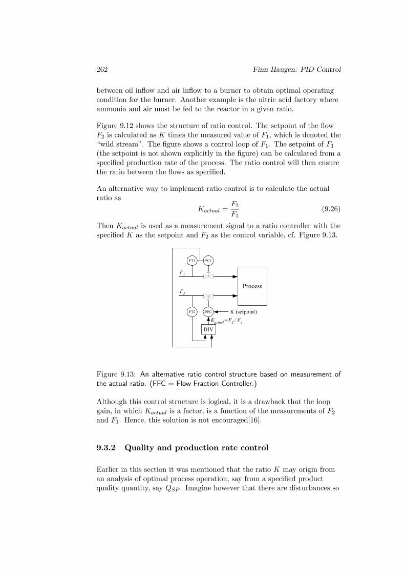
An alternative way to implement ratio control is to calculate the actualratio as

Kactual =F2F1

(9.26)

Then Kactual is used as a measurement signal to a ratio controller with thespecified K as the setpoint and F2 as the control variable, cf. Figure 9.13.

Process

FT1

FFCFT2

DIV

K (setpoint)Kactual =F2 / F1

F1

F2

FC1

Figure 9.13: An alternative ratio control structure based on measurement ofthe actual ratio. (FFC = Flow Fraction Controller.)

Although this control structure is logical, it is a drawback that the loopgain, in which Kactual is a factor, is a function of the measurements of F2and F1. Hence, this solution is not encouraged[16].

9.3.2 Quality and production rate control

Earlier in this section it was mentioned that the ratio K may origin froman analysis of optimal process operation, say from a specified productquality quantity, say QSP . Imagine however that there are disturbances so


that key components in one of or in both flows F1 or F2 vary somewhat.Due to such disturbances it may well happen that the actual productquality is different from QSP . Such disturbances may also cause the actualproduct flow to differ from a flow setpoint. These problems can be solvedby implementing

• a quality control loop based on feedback from measured quality Q tothe ratio parameter K, and

• a product flow control loop based on feedback from measured flow Fto one of the feed flows.

Figure 9.14 shows the resulting quality and production rate control system.

Process

FT1

FC2FT2

MULT

K

K F1 = F2SP

F1

MeasuredF1

F2

Wild stream

FC1

QT

QC

Quality control loop

Qualitysetpoint

QSP

FT

FCFSP

Product

Flow control loop

Figure 9.14: Control of quality and product flow. (QT = Quality Transmitter.QC = Quality Controller.)

9.4 Split-range control

In split-range control one controller controls two actuators in differentranges of the control signal span, which here is assumed to be 0 — 100%.See Figure 9.15. Figure 9.16 shows an example of split-range temperaturecontrol of a thermal process. Two valves are controlled — one for coolingand one for heating, as in a reactor. The temperature controller controls


50 % 100 %0 %

Open

Control variable, u

Closed

Valve position

Valve Vc Valve Vh

Valve VcValve Vh

Figure 9.15: Split-range control of two valves

the cold water valve for control signals in the range 0—50%, and it controlsthe hot water valve for control signals in the range 50—100%, cf. Figure9.15.

In Figure 9.15 it is indicated that one of the valves are open while theother is active. However in certain applications one valve can still be openwhile the other is active, see Figure 9.17. One application is pressurecontrol of a process: When the pressure drop compensation is small (aswhen the process load is small), valve V1 is active and valve V2 is closed.And when the pressure drop compensation is is large (as when the processload is large), valve V1 is open and valve V2 is still active.

9.5 Control of product flow and mass balance ina plant

In the process industry products are created after treatment of thematerials in a number of stages in series, which are typically unit processesas blending or heated tanks, buffer tanks, distillation columns, absorbers,reactors etc. The basic control requirements of such a production line areas follows:

• The mass flow of a key component must be controlled, that is, tofollow a given production rate or flow setpoint.


Process

TTTC

ValveVc

Vh

Cold water

Hot water

Figure 9.16: Split-range temperature control using two control valves

50 % 100 %0 %

Open

Control signal, u

Closed

Valve position

Valve V1

Valve V2

Figure 9.17: In split-range control one valve can be active while another valveis open simultaneuously.

• The mass balance in each process unit (tank etc.) must bemaintained — otherwise e.g. the tank may go full or empty.

Figure 9.18 shows the principal control system structure to satisfy theserequirements. (It is assumed that the mass is proportional to the level.)The position of the production flow control in the figure is just oneexample. It may be placed earlier (or later) in the line depending on wherethe key component(s) are added.

Note that the mass balance of an upstream tank (relative to theproduction flow control) is controlled by manipulating the mass inflow tothe tank, while the mass balance of a downstream tank is controlled bymanipulating the mass outflow to the tank.


FT

Production flow or ratesetpoint

LC

LT

LC

LT

FC

LC

LT

LC

LT

Downstream tanksUpstream tanks

Figure 9.18: Control of a production line to maintain product flow (rate) andmass balances

In Figure 9.18 the mass balances are maintained using level control. If thetanks contains vapours, the mass balances are maintained using pressurecontrol. Then pressure sensors (PT = Pressure Transmitter) takes theplaces of the level sensors (LT = Level Transmitters), and pressurecontrollers (PC = Pressure Controller) takes the place of level controllers(LC = Level Controller) in Figure 9.18.

Example 9.7 Control of production line

Figure 9.19 shows the front panel of a simulator of a general productionline. The level controllers are PI controllers which are tuned so that thecontrol loops get proper speed and stability (the parameters may becalculated as explained in Chapter 7.2.2). The production flow F is herecontrolled using a PI controller. Figure 9.19 shows how the level controlloops maintain the mass balances (in steady-state) by compensating for adisturbance which is here caused by a change of the production flow. Notethat controller LC2 must have negative gain (i.e. direct action, cf. Section2.6.8) — why?4


4Because the process has negative gain, as an increase of the control signal gives areduction of the level/level measurement.


Figure 9.19: Example 9.7: The level control loops maintain the mass balances(in steady-state).

9.6 Multivariable control

9.6.1 Introduction

Multivariable processes has more than one input variables or ore than oneoutput variables. Here are a few examples of multivariable processes:

• A heated liquid tank where both the level and the temperature shallbe controlled.

• A distillation column where the top and bottom concentration shallbe controlled.

• A robot manipulator where the positions of the manipulators (arms)shall be controlled.

• A chemical reactor where the concentration and the temperatureshall be controlled.

finn haugen: pid control -...

Documents