finite differences: parabolic problems

16.920J/SMA 5212

Numerical Methods for Partial Differential Equations

Lecture 5

Finite Differences: Parabolic Problems

B. C. Khoo

Thanks to Franklin Tan

19 February 2003

16.920J/SMA 5212 Numerical Methods for PDEs

2

OUTLINE • Governing Equation • Stability Analysis • 3 Examples • Relationship between σ and λh • Implicit Time-Marching Scheme • Summary

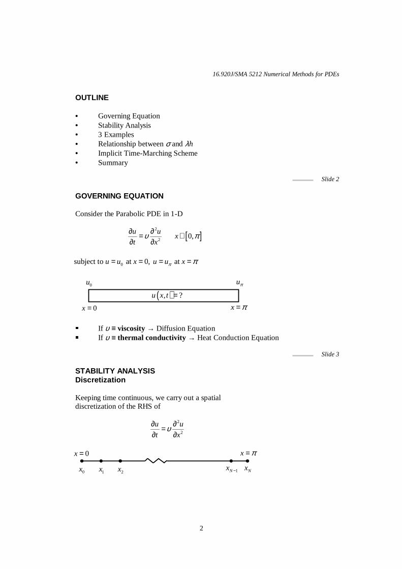
Slide 2 GOVERNING EQUATION Consider the Parabolic PDE in 1-D

� If υ ≡ viscosity → Diffusion Equation� If υ ≡ thermal conductivity → Heat Conduction Equation

Slide 3 STABILITY ANALYSIS Discretization Keeping time continuous, we carry out a spatial discretization of the RHS of

[ ]2

20,

u ux

t xυ π∂ ∂= ∈

∂ ∂

0subject to at 0, at u u x u u xπ π= = = =

0x = x π=

0u uπ

( ), ?u x t =

2

2

u u

t xυ∂ ∂=

∂ ∂

0x = x π=

0x 1x 2x 1Nx − Nx


3

Slide 4

STABILITY ANALYSIS Discretization

which is second-order accurate. • Schemes of other orders of accuracy may be constructed.

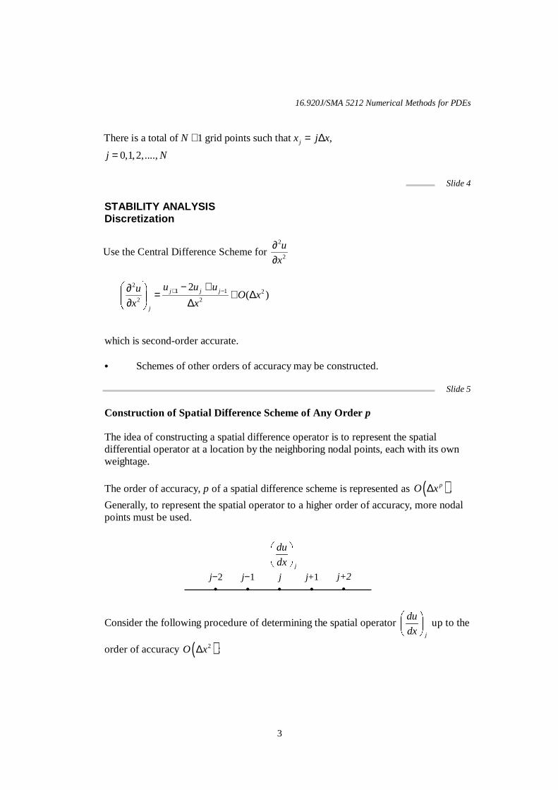
Slide 5 Construction of Spatial Difference Scheme of Any Order p The idea of constructing a spatial difference operator is to represent the spatial differential operator at a location by the neighboring nodal points, each with its own weightage.

The order of accuracy, p of a spatial difference scheme is represented as ( )pO x∆ .

Generally, to represent the spatial operator to a higher order of accuracy, more nodal points must be used.

Consider the following procedure of determining the spatial operator j

du

dx

� �� up to the

order of accuracy ( )2O x∆ :

There is a total of 1 grid points such that ,

0,1,2,....,jN x j x

j N

+ = ∆=

2

2Use the Central Difference Scheme for

u

x

∂∂

21 1 2

2 2

2( )j j j

j

u u uuO x

x x+ −− +

� �∂ = + ∆

�

∂ ∆ �

j−2 •

j−1 •

j •

j+1 •

j+2 •

j

du

dx

� � ��


4

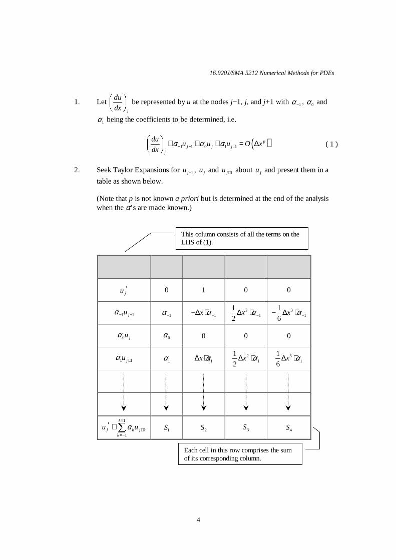
1. Let j

du

dx

� �� be represented by u at the nodes j−1, j, and j+1 with 1α− , 0α and

1α being the coefficients to be determined, i.e.

( )1 1 0 1 1p

j j jj

duu u u O x

dxα α α− − +

� �+ + + = ∆� �

2. Seek Taylor Expansions for 1ju − , ju and 1ju + about ju and present them in a

table as shown below. (Note that p is not known a priori but is determined at the end of the analysis

when the α’ s are made known.)

uj uj′′′′ uj′′′′′′′′ uj′′′′′′′′′′′′

ju ′ 0 1 0 0

1 1juα− − 1α− 1x α−−∆ ⋅ 2

1

1

2x α−∆ ⋅ 3

1

1

6x α−− ∆ ⋅

0 juα 0α 0 0 0

1 1juα + 1α 1x α∆ ⋅ 2

1

1

2x α∆ ⋅ 3

1

1

6x α∆ ⋅

1

1

k

j k j kk

u uα=

+=−

′ + � 1S 2S 3S 4S

( 1 )

This column consists of all the terms on the LHS of (1).

Each cell in this row comprises the sum of its corresponding column.


5

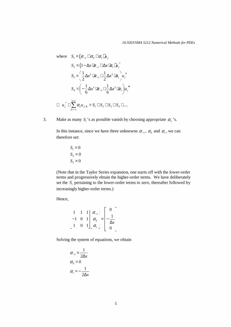
where

∴ 1

1 2 3 41

....k

j k j kk

u u S S S Sα=

+=−

′ + = + + + +�

3. Make as many iS ’ s as possible vanish by choosing appropriate kα ’ s.

In this instance, since we have three unknowns 1α− , 0α and 1α , we can

therefore set:

1

2

3

0

0

0

S

S

S

===

(Note that in the Taylor Series expansion, one starts off with the lower-order

terms and progressively obtain the higher-order terms. We have deliberately set the iS pertaining to the lower-order terms to zero, thereafter followed by

increasingly higher-order terms.) Hence,

1

0

1

01 1 1

11 0 1

1 0 10

x

ααα

−

� �� − = −� � � �

∆� ��

Solving the system of equations, we obtain

1

0

1

1

20

1

2

x

x

α

α

α

− =∆

=

= −∆

( )( )

1 1 0 1

2 1 1

2 23 1 1

3 34 1 1

1

1 1

2 2

1 1

6 6

j

j

j

j

S u

S x x u

S x x u

S x x u

α α α

α α

α α

α α

−

−

−

−

= + +

′= − ∆ ⋅ + ∆ ⋅�

′′= ∆ ⋅ + ∆ ⋅ ��

′′′= − ∆ ⋅ + ∆ ⋅ ��


6

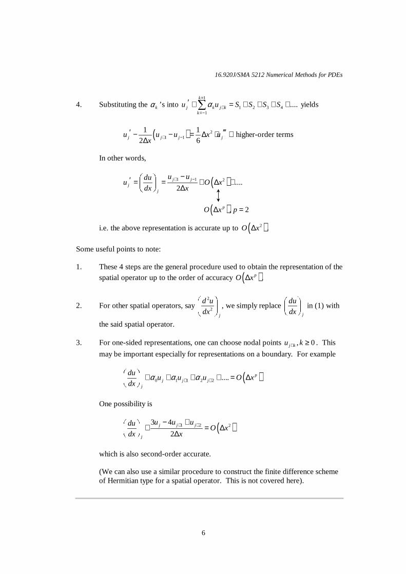
4. Substituting the kα ’ s into 1

1 2 3 41

....k

j k j kk

u u S S S Sα=

+=−

′ + = + + + +�

yields

( ) 21 1

1 1

2 6j j j ju u u x ux + −

′ ′′′− − = ∆ ⋅ +∆

higher-order terms

In other words,

( )1 1 2 ....2

j jj

j

u uduu O x

dx x+ −−

� �′ = = + ∆ +

� �∆

� �

i.e. the above representation is accurate up to ( )2O x∆ .

Some useful points to note: 1. These 4 steps are the general procedure used to obtain the representation of the

spatial operator up to the order of accuracy ( )pO x∆ .

2. For other spatial operators, say 2

2

j

d u

dx

� � � � , we simply replace

j

du

dx

�� in (1) with

the said spatial operator. 3. For one-sided representations, one can choose nodal points , 0j ku k+ ≥ . This

may be important especially for representations on a boundary. For example

( )0 1 1 2 2 .... pj j j

j

duu u u O x

dxα α α+ +

� �+ + + + = ∆� ��

One possibility is

( )1 2 23 4

2j j j

j

u u uduO x

dx x+ +− +

� �+ = ∆� �

∆� �

which is also second-order accurate. (We can also use a similar procedure to construct the finite difference scheme

of Hermitian type for a spatial operator. This is not covered here).

( ) , 2pO x p∆ =


7

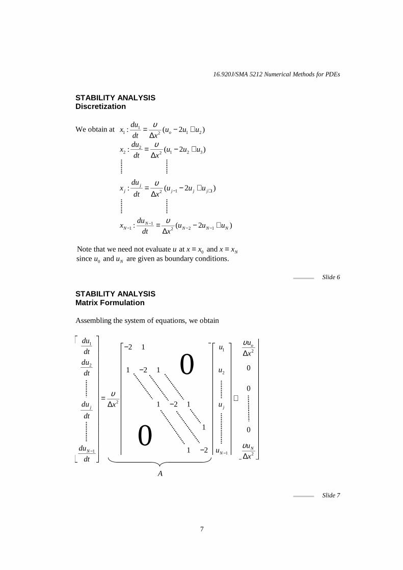
STABILITY ANALYSIS Discretization

We obtain at 11 1 22: ( 2 )o

dux u u u

dt x

υ= − +∆

22 1 2 32

: ( 2 )du

x u u udt x

υ= − +∆

1 12: ( 2 )j

j j j j

dux u u u

dt x

υ− += − +

∆

11 2 12: ( 2 )N

N N N N

dux u u u

dt x

υ−− − −= − +

∆

0

0

Note that we need not evaluate at and since and are given as boundary conditions.

N

N

u x x x xu u

= =

Slide 6

STABILITY ANALYSIS Matrix Formulation Assembling the system of equations, we obtain

Slide 7

1

1 2

2

2

2

1 1 2

2 1

01 2 1

0

1 2 1

1 0

1 2

o

jj

NN N

du uu

dt xdu

udt

udu x

dt

udu uxdt

υ

υ

υ− −

� � � �−

� �� ∆

� �� − � ��

= +� ��

−∆� ��

−� � � ��

∆� ��

��

0

0

A


8

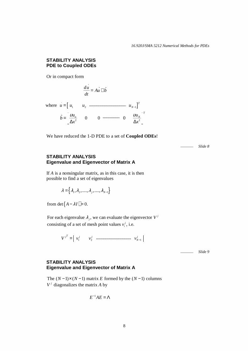
STABILITY ANALYSIS PDE to Coupled ODEs Or in compact form We have reduced the 1-D PDE to a set of Coupled ODEs!

Slide 8 STABILITY ANALYSIS Eigenvalue and Eigenvector of Matrix A If A is a nonsingular matrix, as in this case, it is then possible to find a set of eigenvalues { }1 2 1, ,...., ,....,j Nλ λ λ λ λ −=

( )from det 0.A Iλ− =

For each eigenvalue , we can evaluate the eigenvector

consisting of a set of mesh point values , i.e.

jj

ji

V

v

λ

Slide 9 STABILITY ANALYSIS Eigenvalue and Eigenvector of Matrix A The ( 1) ( 1) matrix formed by the ( 1) columns

diagonalizes the matrix byj

N N E NV A

− × − −

1E AE− = Λ

[ ]1 2 1where T

Nu u u u −=�

2 20 0 0

T

o Nu ub

x x

υ υ� �

= � �∆ ∆� �

�

duAu b

dt= +� ��

1 2 1 Tj j j j

NV v v v −

�= �


9

Slide 10

STABILITY ANALYSIS Coupled ODEs to Uncoupled ODEs

Starting from du

Au bdt

= +� ��

1Premultiplication by yieldsE−

1 1 1duE E Au E b

dt− − −= +

��

Slide 11 STABILITY ANALYSIS Coupled ODEs to Uncoupled ODEs Continuing from

1 1 1duE E u E b

dt− − −= Λ +

��

1 1Let and , we haveU E u F E b− −= =

��

1

2

1

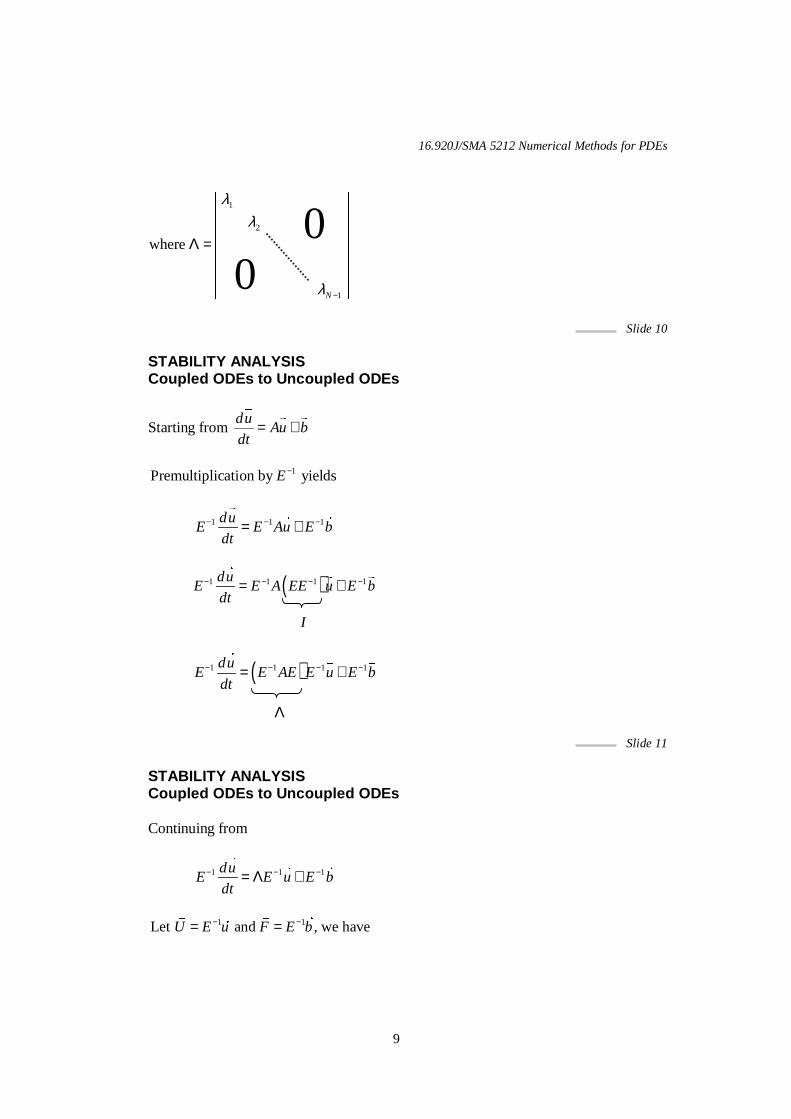
where

N

λλ

λ −

� ��

Λ = � ��

0 0

( )1 1 1 1duE E A EE u E b

dt− − − −= +

��

I

Λ

( )1 1 1 1duE E AE E u E b

dt− − − −= +


10

d

U U Fdt

= Λ +� � � �

�

which is a set of Uncoupled ODEs!

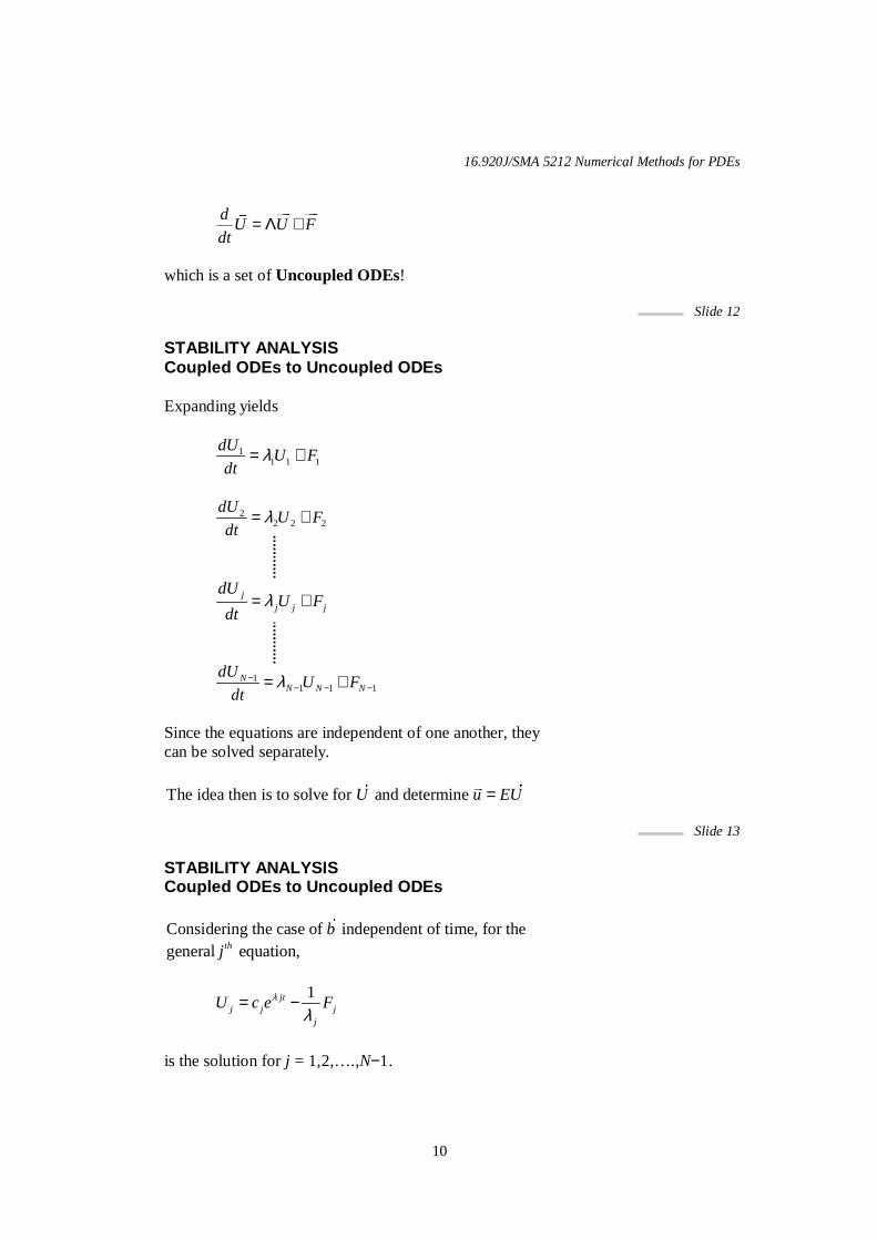
Slide 12 STABILITY ANALYSIS Coupled ODEs to Uncoupled ODEs Expanding yields

11 1 1

dUU F

dtλ= +

22 2 2

dUU F

dtλ= +

jj j j

dUU F

dtλ= +

11 1 1

NN N N

dUU F

dtλ−

− − −= +

Since the equations are independent of one another, they can be solved separately.

The idea then is to solve for and determine U u EU=� �

�

Slide 13 STABILITY ANALYSIS Coupled ODEs to Uncoupled ODEs Considering the case of independent of time, for thegeneral equation,th

bj

�

1jt

j j jj

U c e Fλ

λ= −

is the solution for j = 1,2,….,N−1.


11

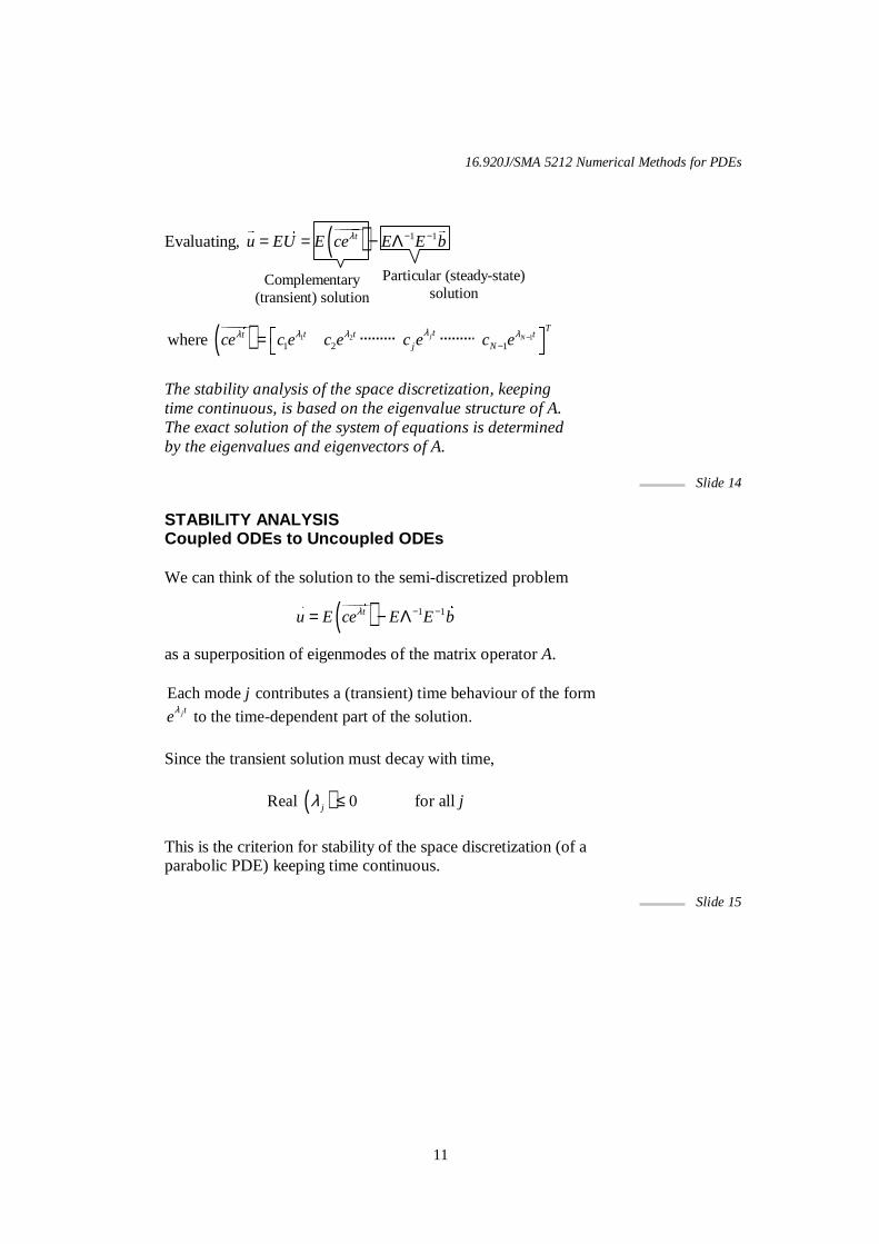
Evaluating, ( ) 1 1tu EU E ce E E bλ − −= = − Λ��

( ) 11 21 2 1where j N

Tt tt ttj Nce c e c e c e c e

λ λλ λλ −−

� �= � �

��

The stability analysis of the space discretization, keeping time continuous, is based on the eigenvalue structure of A. The exact solution of the system of equations is determined by the eigenvalues and eigenvectors of A.

Slide 14 STABILITY ANALYSIS Coupled ODEs to Uncoupled ODEs We can think of the solution to the semi-discretized problem as a superposition of eigenmodes of the matrix operator A. Each mode contributes a (transient) time behaviour of the form

to the time-dependent part of the solution.jt

j

eλ

Since the transient solution must decay with time, ( )Real 0jλ ≤ for all j

This is the criterion for stability of the space discretization (of a parabolic PDE) keeping time continuous.

Slide 15

Complementary (transient) solution

Particular (steady-state) solution

( ) 1 1tu E ce E E bλ − −= − Λ��


12

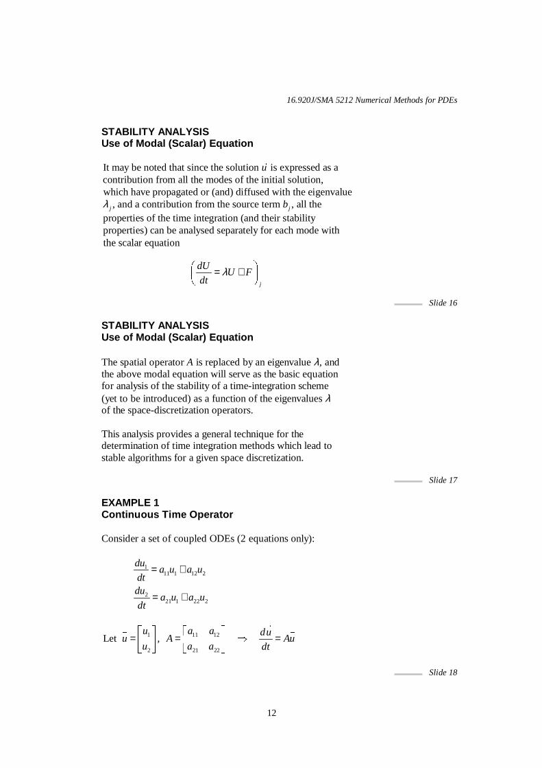
STABILITY ANALYSIS Use of Modal (Scalar) Equation It may be noted that since the solution is expressed as acontribution from all the modes of the initial solution,which have propagated or (and) diffused with the eigenvalue

, and a contribution frj

u

λ

�

om the source term , all theproperties of the time integration (and their stabilityproperties) can be analysed separately for each mode withthe scalar equation

jb

Slide 16 STABILITY ANALYSIS Use of Modal (Scalar) Equation The spatial operator A is replaced by an eigenvalue λ, and the above modal equation will serve as the basic equation for analysis of the stability of a time-integration scheme (yet to be introduced) as a function of the eigenvalues λ of the space-discretization operators. This analysis provides a general technique for the determination of time integration methods which lead to stable algorithms for a given space discretization.

Slide 17 EXAMPLE 1 Continuous Time Operator Consider a set of coupled ODEs (2 equations only):

111 1 12 2

221 1 22 2

dua u a u

dtdu

a u a udt

= +

= +

1 11 12

2 21 22

Let , u a a du

u A Auu a a dt

��

= = � =� � � ��

Slide 18

j

dUU F

dtλ

�

= +� � �


13

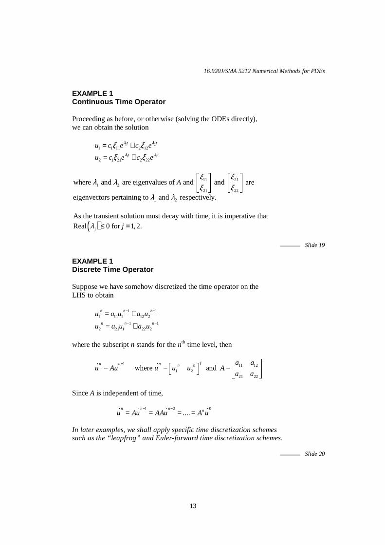
EXAMPLE 1 Continuous Time Operator Proceeding as before, or otherwise (solving the ODEs directly), we can obtain the solution

1 2

1 2

1 1 11 2 12

2 1 21 2 22

t t

t t

u c e c e

u c e c e

λ λ

λ λ

ξ ξξ ξ

= +

= +

11 211 2

21 22

1 2

where and are eigenvalues of and and are

eigenvectors pertaining to and respectively.

Aξ ξ

λ λξ ξ

λ λ

��

( )j

As the transient solution must decay with time, it is imperative thatReal 0 for 1, 2.jλ ≤ =

Slide 19

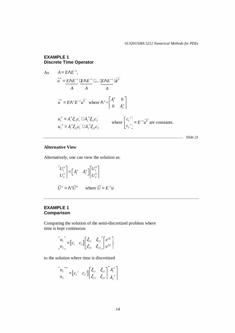
EXAMPLE 1 Discrete Time Operator Suppose we have somehow discretized the time operator on the LHS to obtain

1 1

1 11 1 12 2

1 12 21 1 22 2

n n n

n n n

u a u a u

u a u a u

− −

− −

= +

= +

where the subscript n stands for the nth time level, then

1 11 12

1 221 22

where and Tn n n n n a a

u Au u u u Aa a

− � �� = = = � � � �

Since A is independent of time,

1 2 0

....n n n nu Au AAu A u

− −= = = =� � � �

In later examples, we shall apply specific time discretization schemes such as the “ leapfrog” and Euler-forward time discretization schemes.

Slide 20


14

EXAMPLE 1 Discrete Time Operator As

1 0 1

2

0 where =

0

nn n n

nu E E u

λλ

−

� �= Λ Λ � ��

��

' '

1 1 11 1 2 12 2

' '2 1 21 1 2 22 2

n n n

n n n

u c c

u c c

λ ξ λ ξλ ξ λ ξ

= +

= + 1 1 0

2

'where are constants.

'

cE u

c−

�=

� ��

Slide 21

Alternative View Alternatively, one can view the solution as:

0

1 11 2 0

2 2

nn n

n

U U

U Uλ λ

� � � �� =

� � � ��

0 1where n nU U U E u−= Λ =

� � � �

EXAMPLE 1 Comparison Comparing the solution of the semi-discretized problem where time is kept continuous

[ ]1

2

1 11 121 2

2 21 22

t

t

u ec c

u e

λ

λ

ξ ξξ ξ

� �� = � ��

to the solution where time is discretized

[ ]1 11 12 11 2

2 21 22 2

' 'n n

n

uc c

u

ξ ξ λξ ξ λ

! �! != " #" # " #$�% $ % " #$ %

1

1 1 1 0

,

....n

A E E

u E E E E E E u

−

− − −

= Λ

= Λ ⋅ Λ ⋅ ⋅ Λ ⋅ &'& ((A A A


15

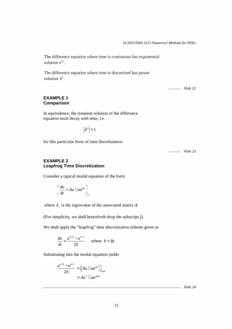
difference equation where time is continuous has exponentialsolution The

.teλ

The difference equation where time is discretized has powersolution .nλ

Slide 22

EXAMPLE 1 Comparison In equivalence, the transient solution of the difference equation must decay with time, i.e. 1nλ <

for this particular form of time discretization.

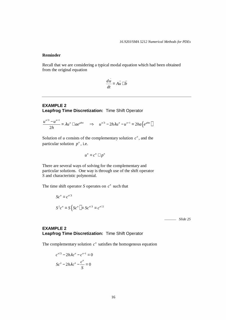
Slide 23 EXAMPLE 2 Leapfrog Time Discretization Consider a typical modal equation of the form

t

j

duu ae

dtµλ

� �

= +� ��

where is the eigenvalue of the associated matrix .j Aλ

(For simplicity, we shall henceforth drop the subscript j).

We shall apply the “ leapfrog” time discretization scheme given as

1 1

where 2

n ndu u uh t

dt h

+ −−= = ∆

Substituting into the modal equation yields

1 1

2

n nu u

h

+ −− ( )t

t nhu aeµλ

== +

n hnu aeµλ= +

Slide 24


16

Reminder Recall that we are considering a typical modal equation which had been obtained from the original equation

duAu b

dt= +��

EXAMPLE 2 Leapfrog Time Discretization: Time Shift Operator

( )1 1

1 1 2 22

n nn hn n n n hnu u

u ae u h u u ha eh

µ µλ λ+ −

+ −− = + � − − =

Solution of u consists of the complementary solution nc , and theparticular solution np , i.e. n n nu c p= + There are several ways of solving for the complementary andparticular solutions. One way is through use of the shift operator S and characteristic polynomial. The time shift operator S operates on nc such that 1n nSc c +=

( )2 1 2n n n nS c S Sc Sc c+ += = =

Slide 25

EXAMPLE 2 Leapfrog Time Discretization: Time Shift Operator The complementary solution nc satisfies the homogenous equation

1 12 0

2 0

n n n

nn n

c h c c

cSc h c

S

λ

λ

+ −− − =

− − =


17

2

2

1( 2 ) 0

( 2 1) 0

n n n

n

S c h Sc cS

cS h S

S

λ

λ

− − =

− − =

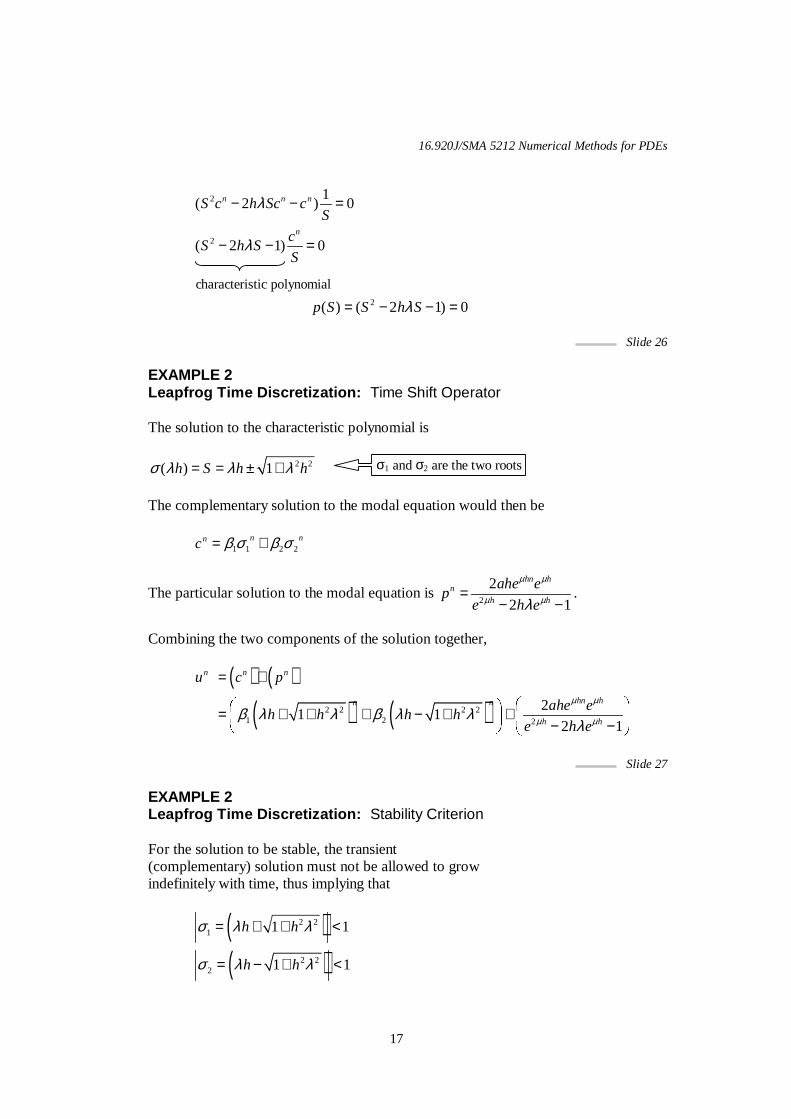
Slide 26 EXAMPLE 2 Leapfrog Time Discretization: Time Shift Operator The solution to the characteristic polynomial is

2 2( ) 1h S h hσ λ λ λ= = ± + The complementary solution to the modal equation would then be 1 1 2 2

n nnc β σ β σ= +

The particular solution to the modal equation is 2

2

2 1

hn hn

h h

ahe ep

e h e

µ µ

µ µλ=

− −.

Combining the two components of the solution together, nu ( ) ( )n nc p= +

( ) ( )2 2 2 21 2 2

21 1

2 1

hn hn n

h h

ahe eh h h h

e h e

µ µ

µ µβ λ λ β λ λλ

� �� = + + + − + + � ��

− −� � � �

Slide 27

EXAMPLE 2 Leapfrog Time Discretization: Stability Criterion For the solution to be stable, the transient (complementary) solution must not be allowed to grow indefinitely with time, thus implying that

( )( )

2 21

2 22

1 1

1 1

h h

h h

σ λ λ

σ λ λ

= + + <

= − + <

characteristic polynomial 2( ) ( 2 1) 0p S S h Sλ= − − =

σ1 and σ2 are the two roots


18

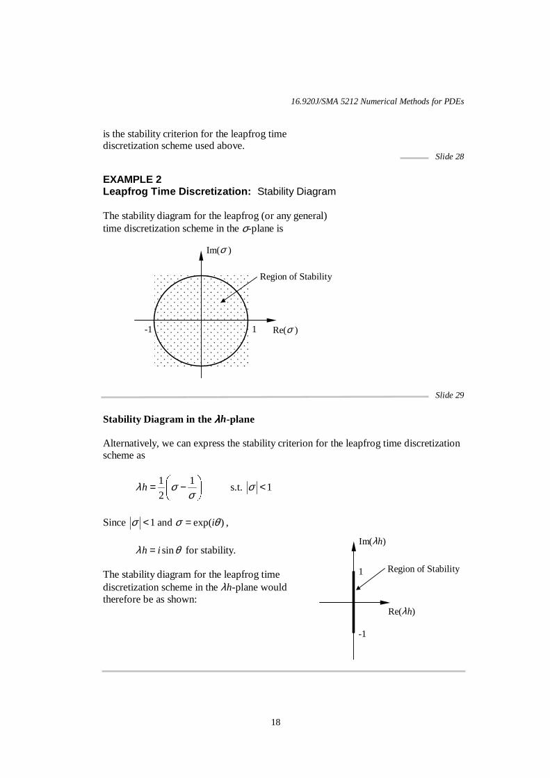
is the stability criterion for the leapfrog time discretization scheme used above.

Slide 28 EXAMPLE 2 Leapfrog Time Discretization: Stability Diagram The stability diagram for the leapfrog (or any general) time discretization scheme in the σ-plane is

Slide 29 Stability Diagram in the λλλλh-plane Alternatively, we can express the stability criterion for the leapfrog time discretization scheme as

1 1

s.t. 12

hλ σ σσ

� �

= − <� ��

Since 1 and exp( )iσ σ θ< = ,

sinh iλ θ= for stability. The stability diagram for the leapfrog time discretization scheme in the λh-plane would therefore be as shown:

Im(σ )

Re(σ ) -1 1

Region of Stability

Re(λh)

Im(λh)

-1

1 Region of Stability


19

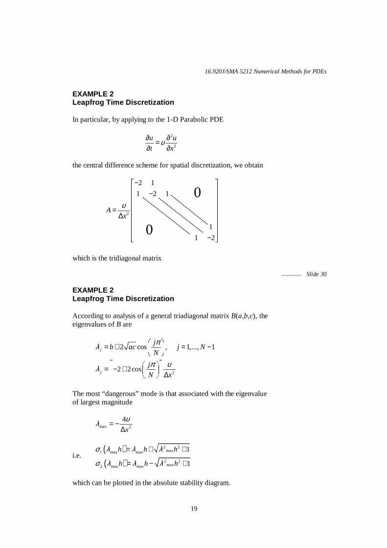
EXAMPLE 2 Leapfrog Time Discretization In particular, by applying to the 1-D Parabolic PDE

2

2

u u

t xυ∂ ∂=

∂ ∂

the central difference scheme for spatial discretization, we obtain which is the tridiagonal matrix

Slide 30 EXAMPLE 2 Leapfrog Time Discretization According to analysis of a general triadiagonal matrix B(a,b,c), the eigenvalues of B are

2

2 cos , 1,..., 1

2 2cos

j

j

jb ac j N

N

j

N x

πλ

π υλ

� �

= + = −� ��

� ��

= − + � ��

∆� � �

The most “dangerous” mode is that associated with the eigenvalue of largest magnitude

max 2

4

x

υλ = −∆

i.e. ( )( )

2 2max1 max max

2 2max2 max max

1

1

h h h

h h h

σ λ λ λ

σ λ λ λ

= + +

= − +

which can be plotted in the absolute stability diagram.

2

2 1

1 2 1

1

1 2

Ax

υ

−� � �

−� ��

=� �

∆ � ��

−� ��

0

0


20

One may note that jλ is always real and negative, thereby satisfying

the criterion for stability of the space discretization of a parabolic PDE, keeping time continuous.

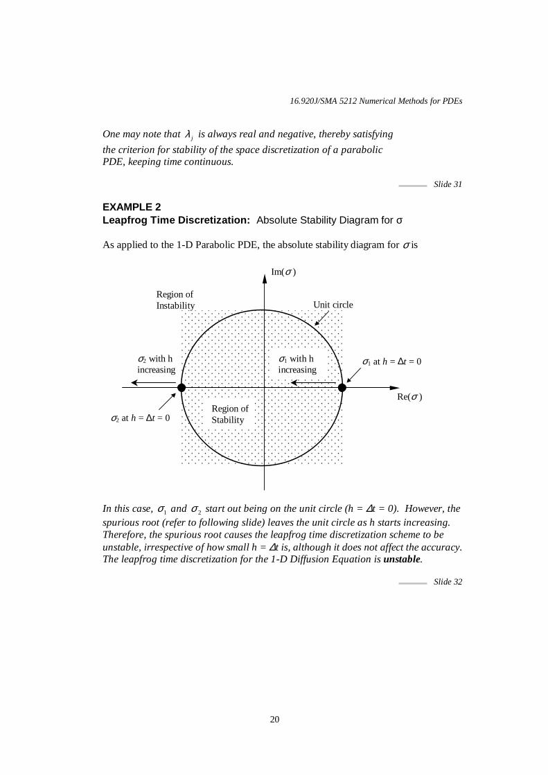
Slide 31 EXAMPLE 2 Leapfrog Time Discretization: Absolute Stability Diagram for σ As applied to the 1-D Parabolic PDE, the absolute stability diagram for σ is In this case, 1σ and 2σ start out being on the unit circle (h = ∆t = 0). However, the spurious root (refer to following slide) leaves the unit circle as h starts increasing. Therefore, the spurious root causes the leapfrog time discretization scheme to be unstable, irrespective of how small h = ∆t is, although it does not affect the accuracy. The leapfrog time discretization for the 1-D Diffusion Equation is unstable.

Slide 32

Im(σ )

Re(σ )

Unit circle

σ1 with h increasing

σ2 with h increasing

Region of Instability

Region of Stability σ2 at h = ∆t = 0

σ1 at h = ∆t = 0


21

STABILITY ANALYSIS Some Important Characteristics Deduced A few features worth considering:

1. Stability analysis of time discretization scheme can be carried out forall the different modes .

2. If the stability criterion for the time discretization scheme is

jλ

valid forall modes, then the overall solution is stable (since it is a linearcombination of all the modes).

3. When there is more than one root , then one of them is the principalroot which represents

σ

( )0

an approximation to the physical behaviour. The principal root is recognized by the fact that it tends towards oneas 0, i.e. lim 1. (The other roots are spurious, which

affect the stability h

h hλ

λ σ λ→

→ =but not the accuracy of the scheme.)

Slide 33

STABILITY ANALYSIS Some Important Characteristics Deduced

1

4. By comparing the power series solution of the principal root to ,one can determine the order of accuracy of the time discretizationscheme. In this example of leapfrog time discretization,

1

he

h

λ

σ λ= + ( ) ( )1

2 2 2 2 4 42

2 2

1

2 2

1 1.1 2 21 .

2 2!

1 ...2

and compared to

1 ...2!

is identical up to the second order of . Hence, the above schemeis said to be second-order accurate.

h

h h h h

hh

he h

h

λ

λ λ λ λ

λσ λ

λλ

λ

−+ = + + +

= + + +

= + + +

Slide 34


22

EXAMPLE 3 Euler-Forward Time Discretization: Stability Analysis Analyze the stability of the explicit Euler-forward time discretization

1n ndu u u

dt t

+ −=∆

as applied to the modal equation

du

udt

λ=

1

1

Substituting where

into the modal equation, we obtain (1 ) 0

n n

n n

duu u h h t

dt

u h uλ

+

+

= + = ∆

− + =

Slide 35

EXAMPLE 3 Euler-Forward Time Discretization: Stability Analysis Making use of the shift operator S

1 (1 ) (1 ) [ (1 )] 0n n n n nc h c Sc h c S h cλ λ λ+ − + = − + = − + = Therefore ( ) 1

and n n

h h

c

σ λ λβσ

= +=

The Euler-forward time discretization scheme is stable if 1 1hσ λ≡ + <

or bounded by 1 s.t. 1 in the -plane.h hλ σ σ λ= − <

Slide 36

characteristic polynomial


23

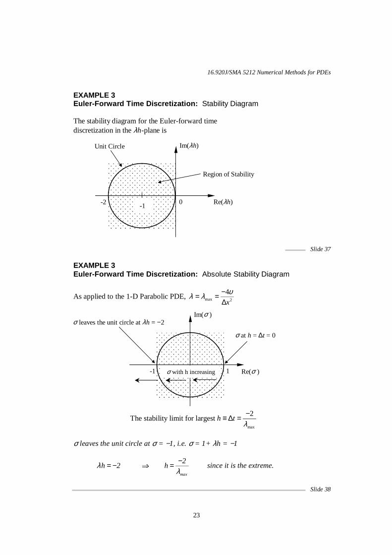
EXAMPLE 3 Euler-Forward Time Discretization: Stability Diagram The stability diagram for the Euler-forward time discretization in the λh-plane is

Slide 37 EXAMPLE 3 Euler-Forward Time Discretization: Absolute Stability Diagram

As applied to the 1-D Parabolic PDE, max 2

4

x

υλ λ −= =∆

max

2The stability limit for largest h t

λ−≡ ∆ =

σ leaves the unit circle at σ = −1, i.e. σ = 1+ λh = −1

max

2h 2 hλ

λ−= − � = since it is the extreme.

Slide 38

Im(λh)

Re(λh) -2 0

Region of Stability

-1

Unit Circle

Im(σ )

-1 1 Re(σ )

σ at h = ∆t = 0

σ leaves the unit circle at λh = −2

σ with h increasing


24

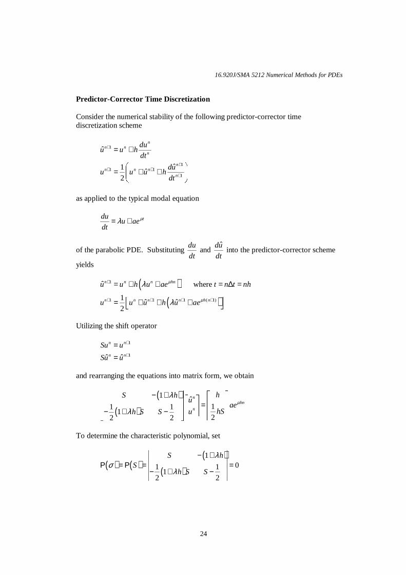
Predictor-Corrector Time Discretization Consider the numerical stability of the following predictor-corrector time discretization scheme

1

11 1

1

ˆ

ˆ1ˆ

2

nn n

n

nn n n

n

duu u h

dt

duu u u h

dt

+

++ +

+

= +� �

= + +� ��

as applied to the typical modal equation

taeudt

du µλ +=

of the parabolic PDE. Substituting dt

du and

dt

ud ˆ into the predictor-corrector scheme

yields

( )

( )

1

1 1 1 ( 1)

ˆ where

1ˆ ˆ

2

n n n hn

n n n n h n

u u h u ae t n t nh

u u u h u ae

µ

µ

λ

λ

+

+ + + +

= + + = ∆ =� �

= + + +�

Utilizing the shift operator

1

1ˆ ˆ

n n

n n

Su u

Su u

+

+

==

and rearranging the equations into matrix form, we obtain

( )

( )

1 ˆ11 1

122 2

nhn

n

hS hu

aehSuh S S

µλ

λ

�− +

�� =

� � �− + − ��

To determine the characteristic polynomial, set

( ) ( )( )

( )

101 1

12 2

S hS

h S S

λσ

λ

− +Ρ = Ρ = =

− + −


25

( ) ( ) 2 2

2 2

11 0

2

0 (trivial root)

11

2

S S S h h

h h

σ λ λ

σ

σ λ λ

� �Ρ = Ρ = − − − =

� �� =

= + +

i.e. the scheme is a one-root method. Compared to

2 211 ....

2he h hλ λ λ= + + +

the scheme is second-order accurate. To obtain the particular solution, one can perform a matrix inversion and obtain

( )

22

21

1

121

hhe

heahep

h

hhn

n

λλ

λ

µ

µµ

−−−

++=

with the complementary solution being

n

nn hhc ��

++== 22

2

11 λλββσ

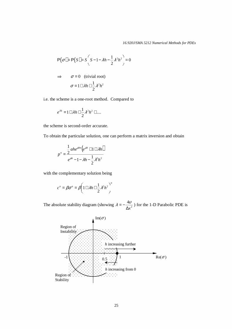
The absolute stability diagram (showing 2

4

x∆−= υλ ) for the 1-D Parabolic PDE is

Im(σ )

Re(σ ) -1 1 0.5

Region of Stabil ity

Region of Instability

h increasing from 0

h increasing further


26

When h increases from zero, σ decreases from 1.0. As h continues to increase, σ reaches a minimum of 0.5 with λh = −1 and then increases. As h increases further, σ returns to 1.0 with λh = −2. Prior to this point, the scheme is stable. Increasing h and thus σ beyond this point renders the scheme unstable. Hence, this predictor-corrector scheme is stable for small h’ s and unstable for large h’ s; the limit for stability is λh = −2 (from above). In general, we can analyze the absolute stability diagram for the predictor-corrector time discretization method in terms of

2( )

: ( ) 12

hh h

λσ σ λ λ= + +

or

: 1 2 1h hλ λ σ= − ± − λ, the eigenvalue(s) of the A matrix can take on complex forms depending on the governing equation (as opposed to negative real values for the 1-D parabolic PDE with central differencing for the spatial derivative).

RELATIONSHIP BETWEEN σσσσ AND λλλλh σσσσ = σσσσ(λλλλh) Thus far, we have obtained the stability criterion of the time discretization scheme using a typical modal equation. We can generalize the relationship between σ and λh as follows: • Starting from the set of coupled ODEs

du

Au bdt

= +�

��

• Apply a specific time discretization scheme like the

leapfrog time discretization as in Example 2

1 1

2

n ndu u u

dt h

+ −−=

Slide 39


27

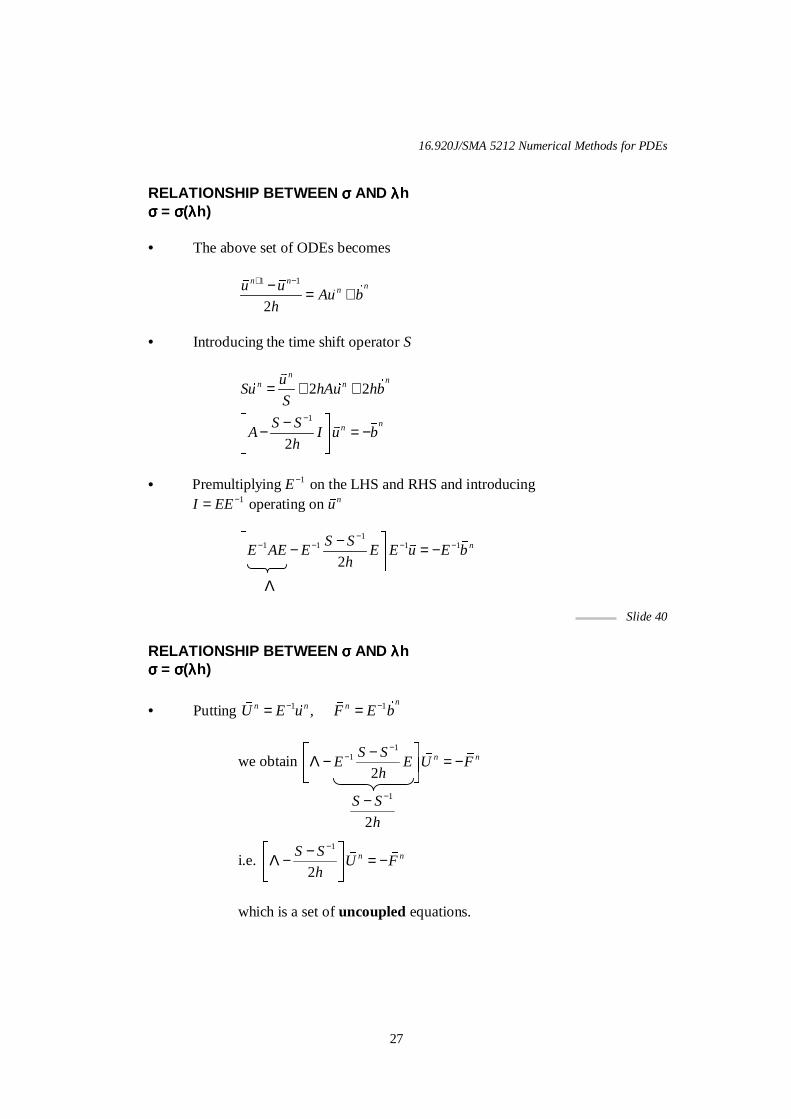
RELATIONSHIP BETWEEN σσσσ AND λλλλh σσσσ = σσσσ(λλλλh) • The above set of ODEs becomes

1 1

2

n nnnu u

Au bh

+ −− = +� � ��

• Introducing the time shift operator S

1

2 2

2

nnn n

nn

uSu hAu hb

S

S SA I u b

h

−

= + +� �

−− = −� ��

� ��

��

•

1

1 1 1 1

2nS S

E AE E E E u E bh

−− − − −

� −− = − �

� ��

Slide 40 RELATIONSHIP BETWEEN σσσσ AND λλλλh σσσσ = σσσσ(λλλλh)

• Putting 1 1,nn n nU E u F E b− −= = ��

we obtain 1

1

2n nS S

E E U Fh

−−

� �−Λ − = −

� ��

i.e. 1

2n nS S

U Fh

−� �

−Λ − = −� ��

which is a set of uncoupled equations.

1

1

Premultiplying on the LHS and RHS and introducing operating on n

EI EE u

−

−= �

Λ

1

2

S S

h

−−


28

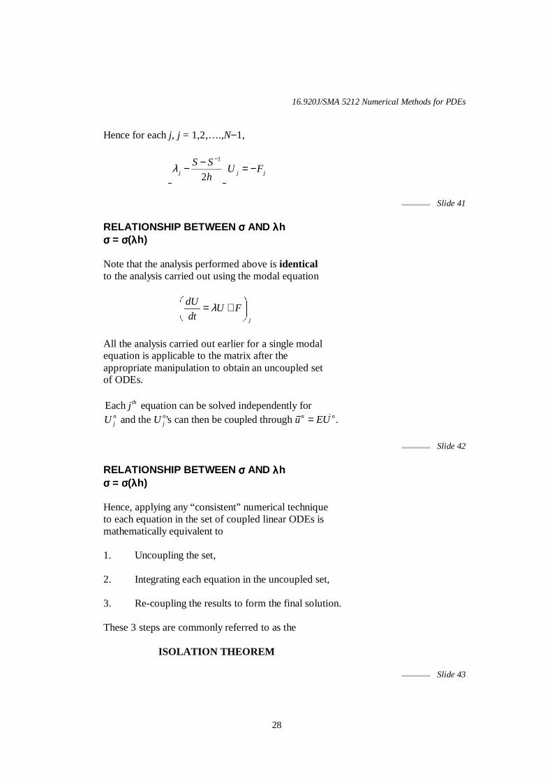
Hence for each j, j = 1,2,….,N−1,

1

2j j j

S SU F

hλ

−� �

−− = −� ��

Slide 41

RELATIONSHIP BETWEEN σσσσ AND λλλλh σσσσ = σσσσ(λλλλh) Note that the analysis performed above is identical to the analysis carried out using the modal equation

j

dUU F

dtλ

� �

= +� �

All the analysis carried out earlier for a single modal equation is applicable to the matrix after the appropriate manipulation to obtain an uncoupled set of ODEs. Each equation can be solved independently for

and the 's can then be coupled through .

th

n n n nj j

jU U u EU= ��

Slide 42

RELATIONSHIP BETWEEN σσσσ AND λλλλh σσσσ = σσσσ(λλλλh) Hence, applying any “consistent” numerical technique to each equation in the set of coupled linear ODEs is mathematically equivalent to 1. Uncoupling the set, 2. Integrating each equation in the uncoupled set, 3. Re-coupling the results to form the final solution. These 3 steps are commonly referred to as the ISOLATION THEOREM

Slide 43


29

IMPLICIT TIME-MARCHING SCHEME Thus far, we have presented examples of explicit time-marching methods and these may be used to integrate weakly stiff equations. Implicit methods are usually employed to integrate very stiff ODEs efficiently. However, use of implicit schemes requires solution of a set of simultaneous algebraic equations at each time-step (i.e. matrix inversion), whilst updating the variables at the same time. Implicit schemes applied to ODEs that are inherently stable will be unconditionally stable or A-stable.

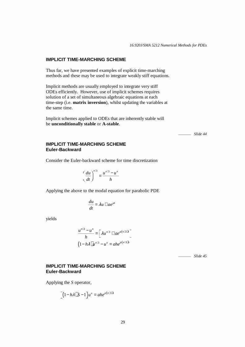
Slide 44 IMPLICIT TIME-MARCHING SCHEME Euler-Backward Consider the Euler-backward scheme for time discretization

1 1n n ndu u u

dt h

+ + −� �

=� ��

Applying the above to the modal equation for parabolic PDE

tduu ae

dtµλ= +

yields

( )

( ) ( )

111

111

n nn hn

n hn n

u uu ae

h

h u u ahe

µ

µ

λ

λ

+++

++

− � �= +�

− − =

Slide 45

IMPLICIT TIME-MARCHING SCHEME Euler-Backward Applying the S operator,

( ) ( )11 1 n hnh S u aheµλ + �

− − =�


30

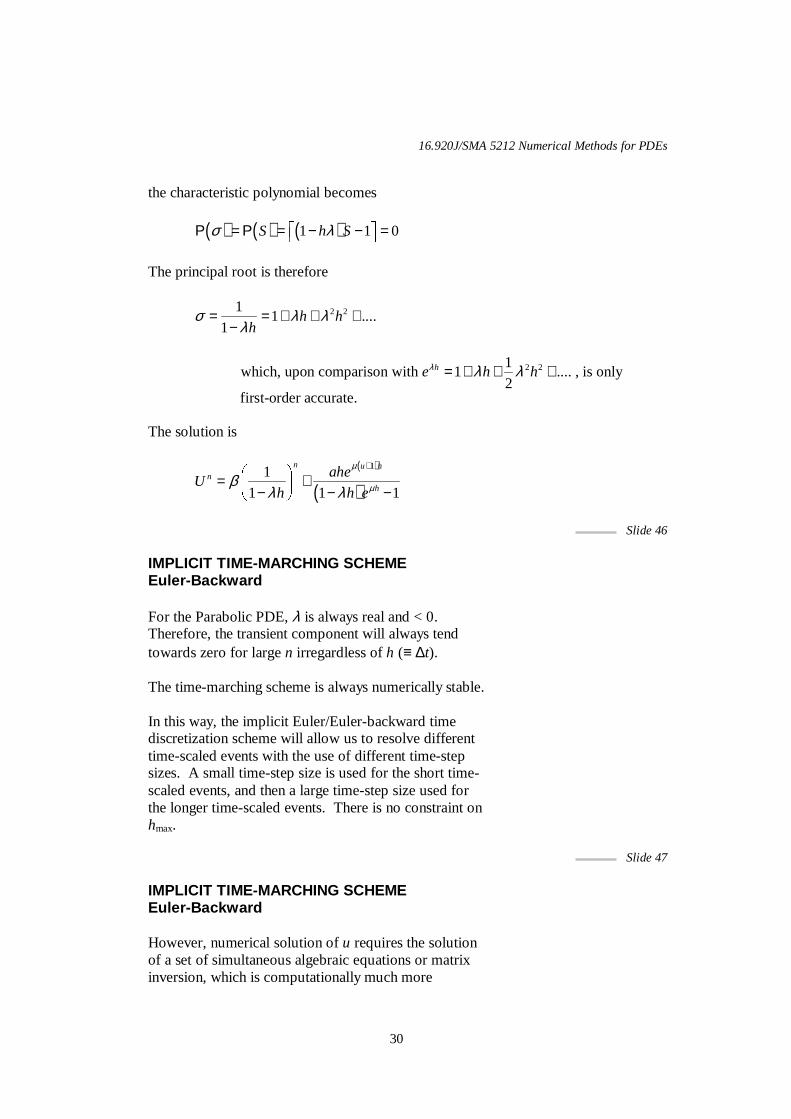
the characteristic polynomial becomes

( ) ( ) ( )1 1 0S h Sσ λ� �

Ρ = Ρ = − − =� �

The principal root is therefore

2 211 ....

1h h

hσ λ λ

λ= = + + +

−

2 21

which, upon comparison with 1 .... , is only2

first-order accurate.

he h hλ λ λ= + + +

The solution is

( )

( )11

1 1 1

n u hn

h

aheU

h h e

µ

µβλ λ

+� �

= +� �

− − −�

Slide 46

IMPLICIT TIME-MARCHING SCHEME Euler-Backward For the Parabolic PDE, λ is always real and < 0. Therefore, the transient component will always tend towards zero for large n irregardless of h (≡ ∆t). The time-marching scheme is always numerically stable. In this way, the implicit Euler/Euler-backward time discretization scheme will allow us to resolve different time-scaled events with the use of different time-step sizes. A small time-step size is used for the short time- scaled events, and then a large time-step size used for the longer time-scaled events. There is no constraint on hmax.

Slide 47 IMPLICIT TIME-MARCHING SCHEME Euler-Backward However, numerical solution of u requires the solution of a set of simultaneous algebraic equations or matrix inversion, which is computationally much more


31

intensive/expensive compared to the multiplication/ addition operations of explicit schemes.

Slide 48 SUMMARY • Stability Analysis of Parabolic PDE

� Uncoupling the set.

� Integrating each equation in the uncoupled set → modal equation.

� Re-coupling the results to form final solution.

• Use of modal equation to analyze the stability |σ(λh)| < 1. • Explicit time discretization versus Implicit time discretization.

Slide 49 Reference: Numerical Computation of Internal and External Flows, Vol I & II by C. Hirsch, 1992, Wiley Series.

finite differences: parabolic problems

Documents