Journal of Computational and Applied Mathematics 35 (1991) 133-138 North-Holland

133

Finite-difference methods for twelfth-order boundary-value problems

A. Boutayeb * and E.H. Twizell Department of Mathematics and Statistics, Brunel University, Uxbridge, Middlesex, United Kingdom UB8 3PH

Received 22 May 1990 Revised 26 November 1990

Abstract

Boutayeb, A. and E.H. Twizell, Finite-difference methods for twelfth-order boundary-value problems, Journal of Computational and Applied Mathematics 35 (1991) 133-138.

The effect of rotation acting on a layer of fluid heated from below is similar to the effect of a magnetic field acting under the same conditions: they both inhibit the onset of instability and they both elongate the cells which appear at marginal stability. However, it must not be assumed that, acting together, rotation and magnetic field reinforce each other. In fact, they have conflicting tendencies when acting together.

The effect of rotation and magnetic field together leads to a twelfth-order eigenvalue problem (Chandrasekhar (1961)) which will be addressed in a future paper.

Experience in solving high-order boundary-value problems has shown that considerable insight may be obtained by solving the special problem first. Moreover, beside the mathematical interest, the computational

aspects of the special problem need to be considered. To this end, finite-difference methods of order two and global extrapolation on two grids are proposed to solve the following special nonlinear twelfth-order boundary- value problem: w”“‘(x) = f(x, w), a < x < b, wC2’)(a) = A,,, wC2”(b) = B,,, i = 0, 1,. . . (5. A simple example is carried out to illustrate the results given by the methods.

Keywords: Twelfth-order boundary-value problems, finite-difference methods, special problem, global extrapola- tion.

1. The second-order method

Consider the special nonlinear twelfth-order boundary-value problem

w@ii)(x) =f(x, w), a<x<b, a, b, XER, (1)

~(~~)(a) = A*,, wczi)( b) = B2,, i=O,l,..., 5. (2)

It is assumed that w(x) and f( x, w) are real and as many times differentiable as required and that A*,, B2,, i=O,l,..., 5, are real finite constants.

Theorems giving the conditions for existence and uniqueness of the solution can be found in [l]. The literature on the numerical solution of twelfth-order boundary-value problems is sparse.

* Present address: Department of Mathematics, Universite Mohamed I, Oujda, Morocco.

0377-0427/91/$03.50 0 1991 - Elsevier Science Publishers B.V. (North-Holland)

134 A. Boutayeb, E.H. TwizeN / Finite-difference methods

Such problems are contained implicitly in [4], although those authors concentrated on numerical methods for fourth-order boundary-value problems. Sixth-order boundary-value problems are solved in [5,6]. The book [3] contains high-order eigenvalue problems with their physical meaning, but no numerical methods are given therein.

One method of solving the above problem is to use second-order replacements of the derivatives directly in (1). This method, which is second-order convergent, can be extrapolated to give higher-order convergence. However, the solution is obtained by solving a nonlinear algebraic system involving a mesh step h raised to the power 12 and the method is likely to suffer from rounding errors [2]. To overcome the word-length problem, the differential equation (1) will be written as a system of six second-order equations:

w,+,(x)=w,“(x), i=l,..., 5, (3)

w;‘(x) =f(x, w,). (4)

The boundary conditions are deduced from (2), (3); they are given by

W,(U) =‘2r-2, w;(b) =Bzi-z> i=l >..a, 6. (5)

Consider, first, the mesh G, obtained by discretizing the interval a < x < b into N + 1 subintervals each of width h = (b - a)/( N + 1) where N is a positive integer. The solution wi( x) will be computed at the mesh points xil) = a + nh, n = 1, 2,. . . , N, of G, and the notation w$) will be adopted to denote the solution of an approximating difference scheme at the grid point x(i) Clearly w;,~ - n *

(1) -A 2i_-2 and w$+i = B2i_2, i = l,.. .,6.

The second-order convergent method (for i = 1,. . . ,6) is given by

- w,“,_i + 2w,(‘,’ - wi”,‘,, + h*w,‘,“’ = 0, (6)

which has local truncation error given by

t_ 1.n

= _ lh4WW 12 r,n - ‘h6w$’ + 0( h*). 360 (7)

Using (6) and the boundary values given in (5), the solution vector W/i) = [ w$), w$,y, . . . , wj,‘,$]‘,

T denoting transpose, is obtained by solving the systems

JiW;” + h*f(‘)( x, I#‘/‘)) = @‘, (8)

J w,(l) + h*W”’ = b(l) 1 I rtl i 3 i=l ,**., 5. (9)

In (8), (9), J, is the familiar tridiagonal matrix of order N given by

2 -1 -1 2 -1

J,= -.f-._-.e

-1 2 -1 -1 2_

(10)

for which 11 Jim’ I( = i( N + 1)2 (the norm referred to throughout this paper is the L, norm). The constant vectors b, are obtained from (5); they are given by bi = ( A2i_2, 0,. . . ,O, B2i_2)T, i = 1 , . . . ,6, and the vector f of order N has the form f(l) = [f{“, fi”‘, . . . , f#‘]‘.

Equations (8), (9) can also be combined to give

J;f,f7;” _ h’*f (1)(x, w;l)) = b(l), 01)

A. Boutayeb, E.H. Twizell / Finite-difference methods 135

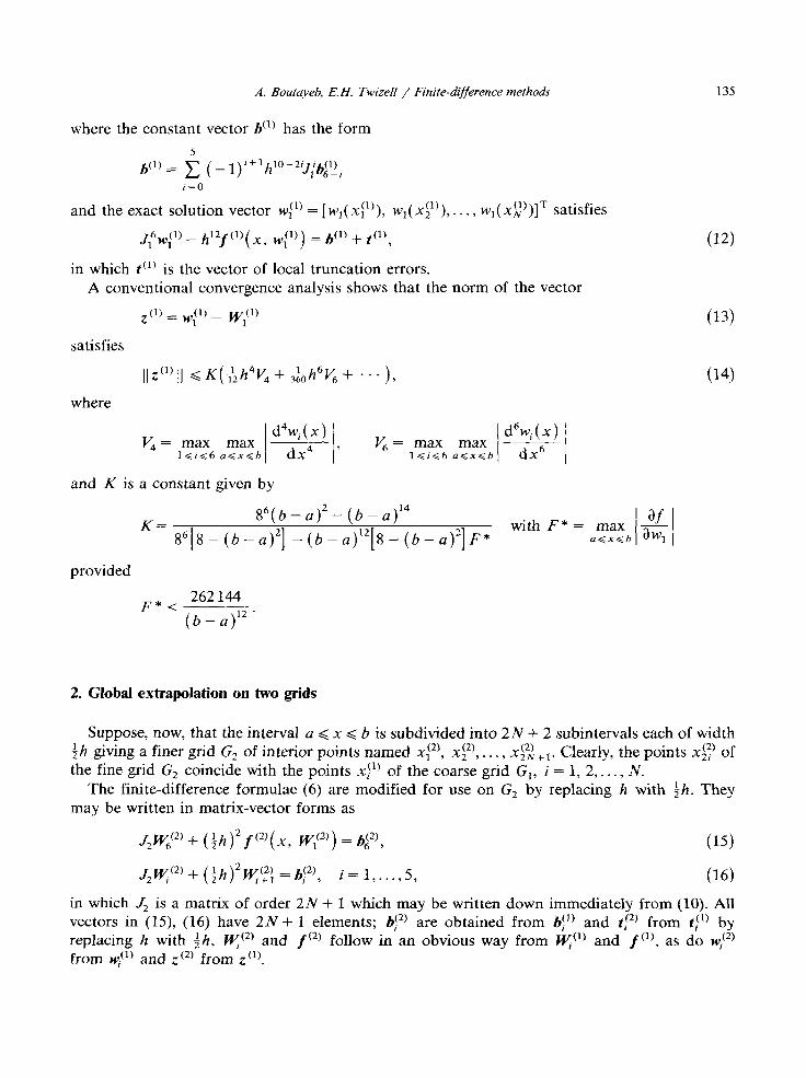
where the constant vector 6(‘) has the form

/p = c ( _ l)‘+‘p2~;p;

i=o

and the exact solution vector w1(t) = [ wl( xl(l)), wl( xi’)), . . . , w,( x!‘)]~ satisfies

~6~0) 1 1

- /!pf(U( .$, wp) = @ + tm,

in which t(‘) is the vector of local truncation errors. A conventional convergence analysis shows that the norm of the vector

z(1) = W,(l) _ wto’

satisfies

where

V, = max max d4wi(x)

i i l&i<6 agx<b dx4 ’ V, = max max

1 ,ci<6 a<x<b

and K is a constant given by

d6w,(x) I I dx6

af with F* = max - a<x<b i I awl

(12)

(13)

04)

provided

F*< 262144

(b - a)12 .

2. Global extrapolation on two grids

Suppose, now, that the interval a < x < b is subdivided into 2N + 2 subintervals each of width ih giving a finer grid G2 of interior points named x,(2), xp’, . . . , x;%+~. Clearly, the points xg’ of the fine grid G2 coincide with the points xj’) of the coarse grid Gt, i = 1, 2,. . . , N.

The finite-difference formulae (6) are modified for use on G, by replacing h with ih. They may be written in matrix-vector forms as

J2W$2) + (+h)’ fc2’( x, W;“) = 6i2’,

J2yc2)+ ($h)‘q$ =!J:~), i= l,..., 5,

(15)

(16)

in which J2 is a matrix of order 2N + 1 which may be written down immediately from (10). All vectors in (15), (16) have 2N+ 1 elements; bt2’ are obtained from b!” and t(‘) from to) by replacing h with $h, wt2) and f (*) follow in’an obvious way from k(l) and ’ f(l), as do w,‘~) from w/l) and zc2) from z(l).

136 A. Boutayeb, E.H. Twizell / Finite-difference methods

In the convergence analysis on G,, zc2) satisfies

11z(2)lj <K(:,($z)2V,+ $&h)“V,+ 0.0).

Introduce, now, an extrapolation vector zcE) of order N defined by

ZCE) = ql;,2z(2) + (1 - q)2”‘,

07)

where I;,2 is a fine-to-coarse grid restriction operator with

I;,2z(2) = [ zi2), zp’, . . . , zizlT and 1j,2W{2) = [ w1(fd, ~$2.. . ~$fl~]~.

Using (1 It,2 II= 1, it follows that

II zCE) II G 4 II zC2) II + (1 - 4) IV) II and that

11 ZCE) 1) = o( h4)

provided

q= $. (18)

The global extrapolation vector

W{E’ = qIj$2Wp + (1 - q) Fp

is thus of order four also.

09)

The nonlinear systems giving the solution of the second-order method and its global extrapola- tion (equations (8), (9) and (15) (16), respectively) are of the form

JF&+ (Q2f(x, tit) =&, (20)

fq+ (&)2e+, =ii, i= l,..., 6, (21)

where f is a matrix of order N or 2N + 1, having the form given by (lo), the vectors q, si, i=l,..., 6, and f* are also of order N or 2 N + 1 and h” takes the value h or ih.

Newton’s method for nonlinear systems may be used to solve (20), (21). Alternatively, these systems can be solved sequentially, using the one-point iteration scheme

.W(k+“+Pj?+, F+(k)) =S, k=O, l).‘. . (22)

To this end, the following algorithm is proposed:

(1) Let W - (‘I be an initial estimate of *. (2) Compute 6 x,_ F+‘)). (3) Estimate S =_66 - g2f”(x, I@(‘)). (4) Solve J”ti = S. (5) Let i = 5. (6) Estimate s”=j, - i2F@. (7) Solve J”ti = S. (8) i=i- 1. (9) If i >P go to_(6).

(10) If II w (O) - w Il < 6 stop. (11) F@(O) = @ and start again with (2).

A. Boutayeb, E.H. Twirell / Finite-difference methods 137

In fact, the implementation of the iteration scheme (22) is more convenient and cheaper than Newton’s method.

3. Numerical results

The following problem was used to test the numerical methods discussed in Sections 1 and 2.

Problem 1.

~(“~~)(x)=ll!*exp{-12w(x)}-2*ll!*(l+x)-~~, 0<x<e’/3-l,

with boundary conditions

and

for which

w(0) = 0, w(e’13 - 1) = $, W(2i)(o) = - (2i - l)!,

W(2i) (e ‘I’-l)=exp(-+i)kvC2’)(0), i=1,...,5,

the theoretical solution is

w(x) = ln(1 +x).

The interval 0 < x G e113 - 1 was divided into N + 1 subintervals each of width h = (e113 -

l)/( N + 1) with N having the values 15, 31 and 63. The results were obtained using the iteration scheme (22) on a Pyramid 9820 computer using FORTRAN with double-precision arithmetic.

For the numerical solutions IV, the error-norm 11 W, - W, (1 was computed for each value of N. The results are given in Table 1 from which it can be seen that decreasing the mesh size improves the results but not as well as does the global extrapolation on two grids.

4. Summary

A second-order finite-difference method and its global extrapolation on two grids have been proposed for the numerical solution of special nonlinear twelfth-order boundary-value problems. The numerical results obtained were seen to be consistent with the orders of convergence of the two formulations.

Table 1 Error norms for the second-order method and its global extrapolation

N Second-order Fourth-order method extrapolation

15 0.195.10-5 0.226.10-* 31 0.492.10-6 0.141.10-9 63 0.123-10-6 0.881.10-”

138 A. Boutayeb, E.H. Twizell / Finite-difference methods

References

[l] R.P. Agarwal, Boundary Value Problems for High Order Differential Equations (World Scientific, Singapore and Philadelphia, 1986).

[2] A. Boutayeb, Numerical methods for high order boundary-value problems, Ph.D. Thesis, Brunel Univ., 1990. [3] S. Chandrasekhar, Hydrodynamic and Hydromagnetic Stability (Clarendon Press, Oxford, 1961); also (Dover, New

York, 1981). [4] M.M. Chawla and C.P. Katti, Finite difference methods for two point boundary-value problems involving higher

order differential equations, BIT 19 (1979) 27-33. [5] E.H. Twizell, Numerical methods for sixth-order boundary-value problems, in: R.P. Agarwal, Y.M. Chow and S.J.

Wilson, Eds., Numerical Mathematics Singapore 1988 (Birkhauser, Basel, 1988) 495-506. [6] E.H. Twizell and A. Boutayeb, Numerical methods for the solution of special and general sixth-order boundary-

value problems, with applications to Btnard layer eigenvalue problems, Proc. Roy. Sot. London Ser. A 431 (1990)

433-450.