finance model guide - energy saving trust · finance model guide ... ‘construction costs’...

Developed by Ricardo-AEA Revision 1 1

Wales Community Renewable Energy Toolkit

Finance Model Guide This guide will enable users to understand and carry out assessments of the indicative financial performance of community renewable energy projects using the Ynni’r Fro Renewables Toolkit Project Finance Model.

Introduction: the Ynni’r Fro Renewables Toolkit Project Finance Model

The Ynni’r Fro Renewables Toolkit Project Finance Model is an indicative early stage financial model to help communities understand the potential profitability of renewable projects, before deciding whether it is worth undertaking further technical and financial due diligence to develop the idea further. At this later stage it will be common for communities to employ their own financial adviser who may assist communities in approaching financiers.

Disclaimer

This model is copyright of the Energy Saving Trust (EST), and is based on an original model developed for the Scottish Government (CARES Model – copyright Scottish Government). With the permission of the Scottish

Government, EST’s consultant, Ricardo-AEA, has adapted the CARES model to produce a model for EST that gives an indicative early stage financial model to help community groups understand the potential profitability of

community renewable investments. Any information and results derived from the use of the EST model are subject to the accuracy of data inputs supplied by the user. All results should be checked and challenged before any reliance, publication or use. This EST model has not been subject to any external independent audit. EST

and Ricardo-AEA hold no liability for any subsequent adjustment or amendments made to the EST model or any loss or damage arising from any reliance on or use of the information generated by the EST model by any

community group, lender, investor or other interested parties.

An additional outcome of filling out the model is that communities will have gathered in a clear format a lot of the necessary financial and project spend information that potential financiers commonly require in their assessments.

Sample data that can be used as a starting point to give a first indication of the scale of the costs and returns that can be expected from a project are provided in Section 0. It does not include sample data for all inputs to the model, only those which must be tailored to each project. The default values for all other inputs can be used at this early stage1. Throughout the development of the project as better estimates become available they should be updated within the model and comments added within the model to reflect this. It would be very unusual for any of the costs outlined below to be present in the final version of the model that is being used to determine if the project is financially viable.

How to use the Ynni’r Fro Renewables Toolkit Finance Model

The sample data that can be used as a starting point to give a first indication of the scale of the costs and returns that can be expected from a project are provided herewith.

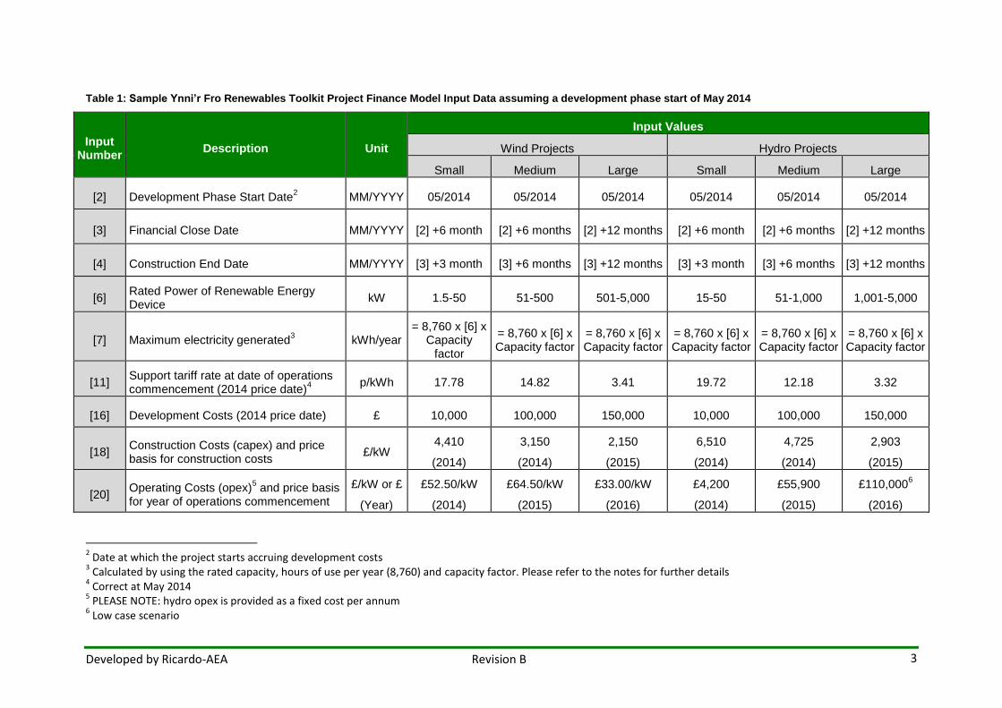
Table 1 provides a summary of inputs to the model for a small (50kW), medium (500kW) and large (1,500kW) wind turbine. There are also inputs for a small (50kW), medium (500kW) and large (2,500kW) hydro project. The figures are aligned with the numbered input cells to the Ynni’r Fro Renewables Toolkit Project Finance Model. Further information is provided below as to how to recalculate these inputs for different installation capacities. The relevant technology section of the Ynni’r Fro Renewables Project Development Toolkit provides

1 The default value for availability factor (input [8]) is discussed later in Section 2.


information on how to go about obtaining actual figures with more representative input data for a project, so that it is not necessary to rely on estimates.

The sample data provided here was taken from a report produced for the Department of Energy and Climate Change (DECC) to update the cost and performance inputs of DECC’s model for the UK Feed-In Tariff (FIT) (Update of non-PV data for Feed in Tariff). This report contains the detailed methodology used in evaluating the costs and performance data which is taken from a number of sources including:

• market intelligence received from DECC (both formal responses to the consultation on Phase 2B of the FITs Comprehensive Review and data received through other channels);

• data on actual capital costs for recent installations, and recent quotes for proposed installations, sourced from a number of different companies; and

• consultation with experts from the industry, including installers, manufacturers, and industry associations.

The DECC report was published in July 2012, and presents cost data in 2012 prices. The Ynni’r Fro Renewables Toolkit Project Finance Model requires all capital costs and development costs to be entered as the actual estimated costs that will be incurred, i.e. taking account of any inflationary cost increases. It also requires operating costs to be entered as the operating costs in the first year of operations (which could rise in a year or two’s time) again taking account of any inflationary increases between now and operations commencement.

As a simplification, it has been assumed that capital and operating costs have risen by 5% between 2012 and 2014. As the first year of operations may be a year or two after the development phase of a project starts it is assumed that if the first year of operations is in 2015 then operating costs will be 7.5% above 2012 prices, and if 2016 is the first year of operations these costs will be 10% above 2012 prices. Communities will obtain more accurate estimates when their project is sufficiently advanced to start engaging with possible providers of renewable energy technologies.

https://www.gov.uk/government/uploads/system/uploads/attachment_data/file/42912/5900-update-of-nonpv-data-for-feed-in-tariff-.pdf

3 Developed by Ricardo-AEA Revision B

Table 1: Sample Ynni’r Fro Renewables Toolkit Project Finance Model Input Data assuming a development phase start of May 2014

Input Number

Description Unit

Input Values

Wind Projects Hydro Projects

Small Medium Large Small Medium Large

[2] Development Phase Start Date2 MM/YYYY 05/2014 05/2014 05/2014 05/2014 05/2014 05/2014

[3] Financial Close Date MM/YYYY [2] +6 month [2] +6 months [2] +12 months [2] +6 month [2] +6 months [2] +12 months

[4] Construction End Date MM/YYYY [3] +3 month [3] +6 months [3] +12 months [3] +3 month [3] +6 months [3] +12 months

[6] Rated Power of Renewable Energy Device

kW 1.5-50 51-500 501-5,000 15-50 51-1,000 1,001-5,000

[7] Maximum electricity generated3 kWh/year

= 8,760 x [6] x Capacity

factor

= 8,760 x [6] x Capacity factor





[11] Support tariff rate at date of operations commencement (2014 price date)

4

p/kWh 17.78 14.82 3.41 19.72 12.18 3.32

[16] Development Costs (2014 price date) £ 10,000 100,000 150,000 10,000 100,000 150,000

[18] Construction Costs (capex) and price basis for construction costs

£/kW 4,410

(2014)

3,150

(2014)

2,150

(2015)

6,510

(2014)

4,725

(2014)

2,903

(2015)

[20] Operating Costs (opex)

5 and price basis

for year of operations commencement

£/kW or £

(Year)

£52.50/kW

(2014)

£64.50/kW

(2015)

£33.00/kW

(2016)

£4,200

(2014)

£55,900

(2015)

£110,0006

(2016)

2 Date at which the project starts accruing development costs

3 Calculated by using the rated capacity, hours of use per year (8,760) and capacity factor. Please refer to the notes for further details

4 Correct at May 2014

5 PLEASE NOTE: hydro opex is provided as a fixed cost per annum

6 Low case scenario


Summary of Input Data for Wind Projects

The following input values can be used in an early stage, high level wind project assessment. These cells are highlighted in green in column B of the ‘Inputs’, ‘Development Costs’ and ‘Construction Costs’ worksheet of the Ynni’r Fro Renewables Toolkit Project Finance Model spreadsheet and must be populated for the model to complete a calculation. For all others cells, highlighted in orange, the default value is sufficient. The numbers assume a development phase start of May 2014. For later start dates higher costs may be appropriate to take account of inflationary increases.

For a detailed financial assessment of the project, all relevant green and orange cells need to be populated with project specific values.

Model input number [2]: Development Phase Start Date (‘Inputs’ worksheet)

This is the first date the project starts incurring development costs. The model assumes the Development Phase starts on the last day of a month to avoid interest costs in that month. Enter the date in the MM/YYYY format and the actual end month date is automatically calculated (shown in cell E7 of worksheet ‘Inputs’).

Model input number [3]: Financial Close Date (‘Inputs’ worksheet)

This is the date when all development costs have been finalised and construction is commenced. The model assumes Financial Close, the date the project documents all get signed and banks offer loans on the main project, occurs on the last day of a month to avoid interest costs in that month. Enter the date in the MM/YYYY format and the actual end month date is automatically calculated (shown in cell E9 of the ‘Inputs’ worksheet).

Depending on the size of the turbine (see Model input number [6] below) this date can be calculated from the Development Phase Start Date using the following assumptions:

Category Duration (months)

Small 67

Medium 6

Large 12+

For example, when calculating the Financial Close Date of a medium size (60kW) project that has the Development Phase Start Date at 05/2014, the Financial Close Date will be 11/2014.

Model input number [4]: Construction End Date (‘Inputs’ worksheet)

The Construction End Date of the project, when commissioning is completed, is assumed to occur at the end of a month. Enter the date in the MM/YYYY format and the actual end month date is automatically calculated (shown in cell E11 of the ‘Inputs’ worksheet). The next day, operations start.

This date can be calculated from the Financial Close Date using the same methodology as for Model input number [3] above and the values in the table below.


Small 3

7 Note that the development duration will vary greatly depending on the capacity size. For example, a 5kW

which would not require planning would have a duration of 1 month


Medium 6

Large 12+

The model assumes typical development period and construction periods will be evaluated. As a result

the maximum total development and construction period is limited to 5 years and 7 months.

Model input number [6]: Rated Power of Renewable Energy Device (kW) (‘Inputs’ worksheet)

The input required here is the capacity of the renewable energy device in kW. The Ynni’r Fro Renewables Toolkit Wind Module provides further information on how to obtain a representative estimate before employing specialist support.

The rated power of projects has been used to create a set of bandings to enable categorisation of projects. This banding is used throughout this document and is categorised using the following bandings:

Category Band

Small 1.5 – 50kW

Medium 51 – 500kW

Large 501 –

5,000kW

These bandings have been created, to align with the estimates of capital costs taken from the source material.

For further information and greater breakdown on project sizing and bandings please refer to the DECC report: Update of non-PV data for Feed in Tariff.

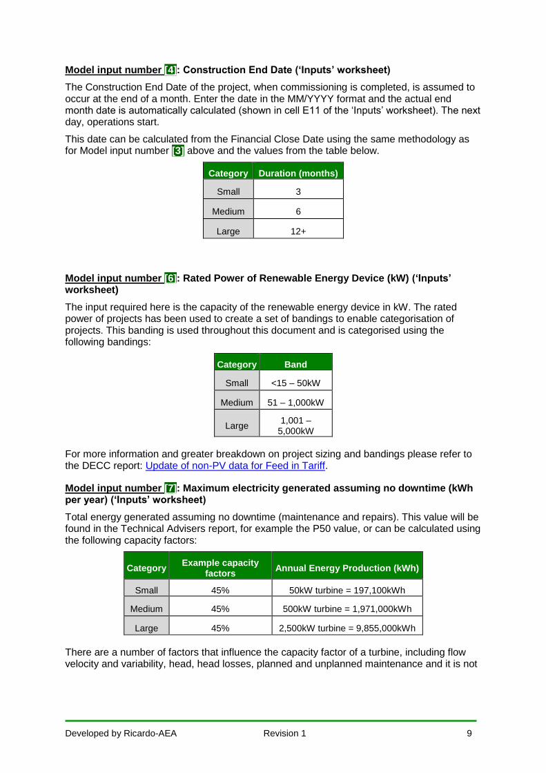
Model input number [7]: Maximum electricity generated assuming no downtime (kWh per year) (‘Inputs’ worksheet)

Total annual electricity generated is the amount of annual electricity that would be generated assuming no downtime (for planned or unplanned maintenance). This value will be found in the Technical Advisers report, for example look for the P50 value. If these figures are not available, an estimate using the following example capacity factors (CF) can be made:

Category Example capacity

factors Annual Energy Production (kWh)

Small 26% (@ 6.5 m/s) 50kW turbine = 113,880kWh

Medium 27% (@ 6.5 m/s) 500kW turbine = 1,182,600kWh

Large 32% (@ 6.5 m/s) 1,500kW turbine = 4,204,800kWh

These will give a rough indicative estimate of the total annual energy generated at a site by a small, medium of large wind turbine. If you know the size of your turbine and the capacity factor, you can calculate the annual electricity generated.

There are a significant number of factors that influence the capacity factor of a turbine, including turbine planned and unplanned maintenance, wind speed, direction and variability, turbine location and turbine height and it is not possible to give an accurate indication of the



capacity factor to enter into the finance model without this information. Hence the figures provided in the table are rough estimates taken from a DECC report8.

For more detailed information and greater breakdown on capacity factors at different wind speeds and for different cases please refer to the DECC report: Update of non-PV data for Feed in Tariff.

To calculate the electricity generation for a turbine of a different rating than ratings above, the following equation should be employed:

𝐺𝑒𝑛𝑒𝑟𝑎𝑡𝑖𝑜𝑛 (𝑘𝑊ℎ) = 𝑅𝑎𝑡𝑒𝑑 𝑐𝑎𝑝𝑎𝑐𝑖𝑡𝑦 (𝑘𝑊) ∗ 8,760(ℎ𝑜𝑢𝑟𝑠) ∗ 𝐶𝐹(%)

Therefore, to calculate the generation in kWh of a system sized 50kW, the calculation would be 50 x 8,760 x 0.28 = 122,640kWh (given the CF of 28% from the table above).

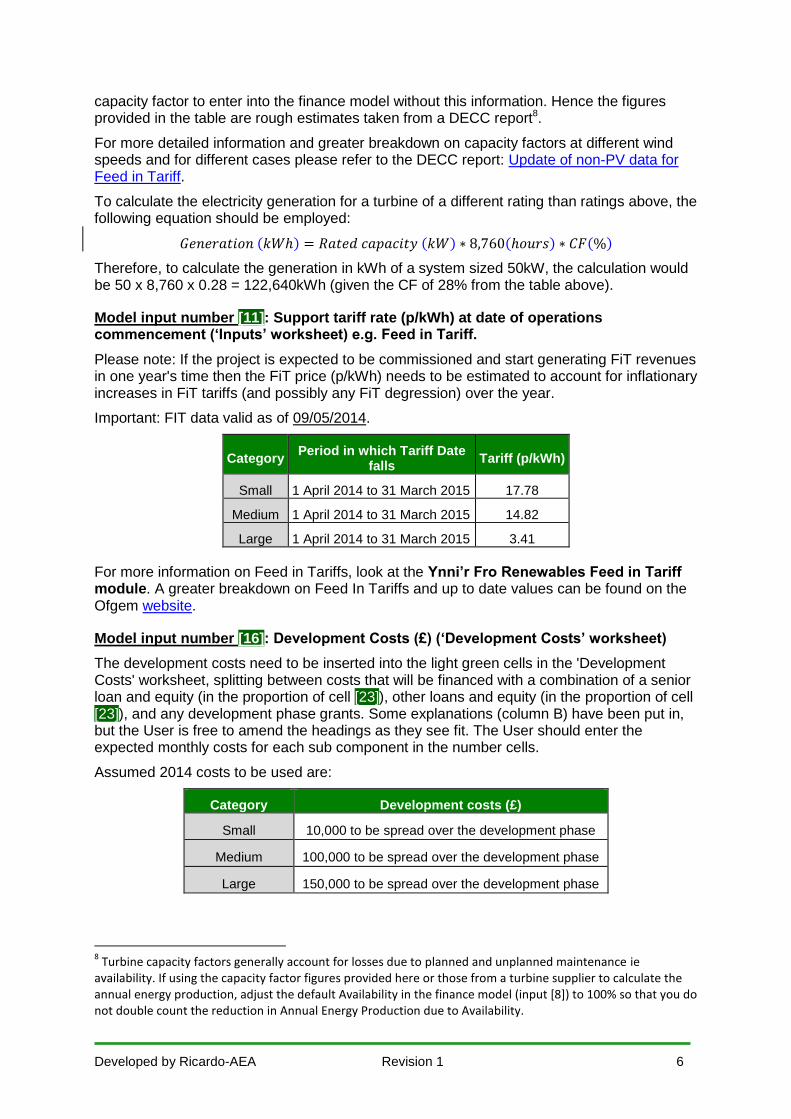
Model input number [11]: Support tariff rate (p/kWh) at date of operations commencement (‘Inputs’ worksheet) e.g. Feed in Tariff.

Please note: If the project is expected to be commissioned and start generating FiT revenues in one year's time then the FiT price (p/kWh) needs to be estimated to account for inflationary increases in FiT tariffs (and possibly any FiT degression) over the year.

Important: FIT data valid as of 09/05/2014.

Category Period in which Tariff Date

falls Tariff (p/kWh)

Small 1 April 2014 to 31 March 2015 17.78

Medium 1 April 2014 to 31 March 2015 14.82

Large 1 April 2014 to 31 March 2015 3.41

For more information on Feed in Tariffs, look at the Ynni’r Fro Renewables Feed in Tariff module. A greater breakdown on Feed In Tariffs and up to date values can be found on the Ofgem website.

Model input number [16]: Development Costs (£) (‘Development Costs’ worksheet)

The development costs need to be inserted into the light green cells in the 'Development Costs' worksheet, splitting between costs that will be financed with a combination of a senior loan and equity (in the proportion of cell [23]), other loans and equity (in the proportion of cell [23]), and any development phase grants. Some explanations (column B) have been put in, but the User is free to amend the headings as they see fit. The User should enter the expected monthly costs for each sub component in the number cells.

Assumed 2014 costs to be used are:

Category Development costs (£)

Small 10,000 to be spread over the development phase

Medium 100,000 to be spread over the development phase

Large 150,000 to be spread over the development phase

8 Turbine capacity factors generally account for losses due to planned and unplanned maintenance ie

availability. If using the capacity factor figures provided here or those from a turbine supplier to calculate the annual energy production, adjust the default Availability in the finance model (input [8]) to 100% so that you do not double count the reduction in Annual Energy Production due to Availability.



https://www.ofgem.gov.uk/environmental-programmes/feed-tariff-fit-scheme/tariff-tables


Please note: this worksheet automatically updates dates from development phase start to the date of financial close. Please ensure that no numbers appear outside the green box. This will mean that if the Development Phase Start Date [2] or Financial Close Date [3] changes in a scenario this worksheet will need to be updated.

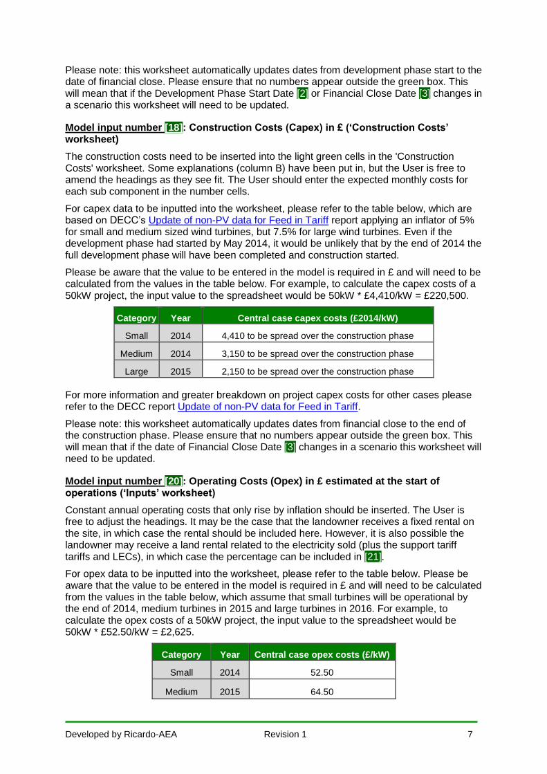
Model input number [18]: Construction Costs (Capex) in £ (‘Construction Costs’ worksheet)

The construction costs need to be inserted into the light green cells in the 'Construction Costs' worksheet. Some explanations (column B) have been put in, but the User is free to amend the headings as they see fit. The User should enter the expected monthly costs for each sub component in the number cells.

For capex data to be inputted into the worksheet, please refer to the table below, which are based on DECC’s Update of non-PV data for Feed in Tariff report applying an inflator of 5% for small and medium sized wind turbines, but 7.5% for large wind turbines. Even if the development phase had started by May 2014, it would be unlikely that by the end of 2014 the full development phase will have been completed and construction started.

Please be aware that the value to be entered in the model is required in £ and will need to be calculated from the values in the table below. For example, to calculate the capex costs of a 50kW project, the input value to the spreadsheet would be 50kW * £4,410/kW = £220,500.

Category Year Central case capex costs (£2014/kW)

Small 2014 4,410 to be spread over the construction phase

Medium 2014 3,150 to be spread over the construction phase

Large 2015 2,150 to be spread over the construction phase

For more information and greater breakdown on project capex costs for other cases please refer to the DECC report Update of non-PV data for Feed in Tariff.

Please note: this worksheet automatically updates dates from financial close to the end of the construction phase. Please ensure that no numbers appear outside the green box. This will mean that if the date of Financial Close Date [3] changes in a scenario this worksheet will need to be updated.

Model input number [20]: Operating Costs (Opex) in £ estimated at the start of operations (‘Inputs’ worksheet)

Constant annual operating costs that only rise by inflation should be inserted. The User is free to adjust the headings. It may be the case that the landowner receives a fixed rental on the site, in which case the rental should be included here. However, it is also possible the landowner may receive a land rental related to the electricity sold (plus the support tariff tariffs and LECs), in which case the percentage can be included in [21].

For opex data to be inputted into the worksheet, please refer to the table below. Please be aware that the value to be entered in the model is required in £ and will need to be calculated from the values in the table below, which assume that small turbines will be operational by the end of 2014, medium turbines in 2015 and large turbines in 2016. For example, to calculate the opex costs of a 50kW project, the input value to the spreadsheet would be 50kW * £52.50/kW = £2,625.

Category Year Central case opex costs (£/kW)

Small 2014 52.50

Medium 2015 64.50




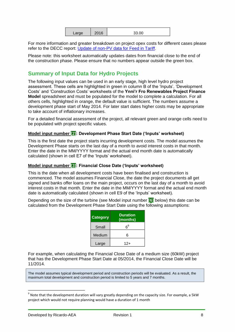
Large 2016 33.00

For more information and greater breakdown on project opex costs for different cases please refer to the DECC report: Update of non-PV data for Feed in Tariff.

Please note: this worksheet automatically updates dates from financial close to the end of the construction phase. Please ensure that no numbers appear outside the green box.

Summary of Input Data for Hydro Projects

The following input values can be used in an early stage, high level hydro project assessment. These cells are highlighted in green in column B of the ‘Inputs’, ‘Development Costs’ and ‘Construction Costs’ worksheets of the Ynni’r Fro Renewables Project Finance Model spreadsheet and must be populated for the model to complete a calculation. For all others cells, highlighted in orange, the default value is sufficient. The numbers assume a development phase start of May 2014. For later start dates higher costs may be appropriate to take account of inflationary increases.

For a detailed financial assessment of the project, all relevant green and orange cells need to be populated with project specific values.

Model input number [2]: Development Phase Start Date (‘Inputs’ worksheet)

This is the first date the project starts incurring development costs. The model assumes the Development Phase starts on the last day of a month to avoid interest costs in that month. Enter the date in the MM/YYYY format and the actual end month date is automatically calculated (shown in cell E7 of the ‘Inputs’ worksheet).

Model input number [3]: Financial Close Date (‘Inputs’ worksheet)

This is the date when all development costs have been finalised and construction is commenced. The model assumes Financial Close, the date the project documents all get signed and banks offer loans on the main project, occurs on the last day of a month to avoid interest costs in that month. Enter the date in the MM/YYYY format and the actual end month date is automatically calculated (shown in cell E9 of the ‘Inputs’ worksheet).

Depending on the size of the turbine (see Model input number [6] below) this date can be calculated from the Development Phase Start Date using the following assumptions:


Small 69

Medium 6

Large 12+

For example, when calculating the Financial Close Date of a medium size (60kW) project that has the Development Phase Start Date at 05/2014, the Financial Close Date will be 11/2014.

The model assumes typical development period and construction periods will be evaluated. As a result, the maximum total development and construction period is limited to 5 years and 7 months.

9 Note that the development duration will vary greatly depending on the capacity size. For example, a 5kW

project which would not require planning would have a duration of 1 month



Model input number [4]: Construction End Date (‘Inputs’ worksheet)

The Construction End Date of the project, when commissioning is completed, is assumed to occur at the end of a month. Enter the date in the MM/YYYY format and the actual end month date is automatically calculated (shown in cell E11 of the ‘Inputs’ worksheet). The next day, operations start.

This date can be calculated from the Financial Close Date using the same methodology as for Model input number [3] above and the values from the table below.


Small 3

Medium 6

Large 12+

Model input number [6]: Rated Power of Renewable Energy Device (kW) (‘Inputs’ worksheet)

The input required here is the capacity of the renewable energy device in kW. The rated power of projects has been used to create a set of bandings to enable categorisation of projects. This banding is used throughout this document and is categorised using the following bandings:

Category Band

Small <15 – 50kW

Medium 51 – 1,000kW

Large 1,001 –

5,000kW

For more information and greater breakdown on project sizing and bandings please refer to the DECC report: Update of non-PV data for Feed in Tariff.

Model input number [7]: Maximum electricity generated assuming no downtime (kWh per year) (‘Inputs’ worksheet)

Total energy generated assuming no downtime (maintenance and repairs). This value will be found in the Technical Advisers report, for example the P50 value, or can be calculated using the following capacity factors:

Category Example capacity

factors Annual Energy Production (kWh)

Small 45% 50kW turbine = 197,100kWh

Medium 45% 500kW turbine = 1,971,000kWh

Large 45% 2,500kW turbine = 9,855,000kWh

There are a number of factors that influence the capacity factor of a turbine, including flow velocity and variability, head, head losses, planned and unplanned maintenance and it is not



possible to give an accurate indication of the capacity factor has to enter into the finance model without this information. Hence the figures provided in the table are rough estimates10.

For more information and greater breakdown on capacity factors for different cases please refer to the DECC report: Update of non-PV data for Feed in Tariff.

To calculate the electricity generation from the capacity factors above, the following equation should be employed:

𝐺𝑒𝑛𝑒𝑟𝑎𝑡𝑖𝑜𝑛 (𝑘𝑊ℎ) = 𝑅𝑎𝑡𝑒𝑑 𝑐𝑎𝑝𝑎𝑐𝑖𝑡𝑦 (𝑘𝑊) ∗ 8760(ℎ𝑜𝑢𝑟𝑠) ∗ 𝐶𝐹(%)

Therefore, to calculate the generation in kWh of a system sized 50kW, the calculation would be 50 x 8,760 x 0.45 = 197,100kWh (given the CF of 45% from the table above).

Model input number [11]: Support tariff rate (p/kWh) at date of operations commencement (‘Inputs’ worksheet) e.g. Feed in Tariff

Please note: if the project is expected to be commissioned and start generating FiT revenues in one year's time then the FiT price (p/kWh) needs to be estimated to account for inflationary increases in FiT tariffs (and possibly any FiT degression) over the year.

Important: FIT data valid as of 09/05/2014.

Category Period in which Tariff Date

falls Tariff (p/kWh)

Small 1 April 2014 to 31 March 2015 19.72

Medium 1 April 2014 to 31 March 2015 12.18

Large 1 April 2014 to 31 March 2015 3.32

For more information and greater breakdown on Feed In Tariffs and up to date values please refer to the Ofgem website.

Model input number [16]: Development Costs (‘Development Costs’ worksheet)

The development costs need to be inserted into the light green cells in worksheet 'Development Costs', splitting between costs that will be financed with a combination of a senior loan and equity (in the proportion of cell [23]), other loans and equity (in the proportion of cell [23]), and any development phase grants. Some explanations (column B) have been put in, but the User is free to amend the headings as they see fit. The User should enter the expected monthly costs for each sub component in the number cells.

Assumed 2014 costs to be used are:

Category Development costs (£)

Small 10,000 to be spread over the development

phase

Medium 100,000 to be spread over the development

phase

Large 150,000 to be spread over the development

phase

10

Turbine capacity factors generally account for losses due to planned and unplanned maintenance ie availability. If using the capacity factor figures provided here or those from a turbine supplier to calculate the annual energy production, adjust the default Availability in the finance model (input [8]) to 100% so that you do not double count the reduction in Annual Energy Production due to Availability.


https://www.ofgem.gov.uk/environmental-programmes/feed-tariff-fit-scheme/tariff-tables


Please note: this worksheet automatically updates dates from development phase start to the date of financial close. This will mean that if the Development Phase Start Date [2] or Financial Close Date [3] changes in a scenario this worksheet will need to be updated. Please ensure that no numbers appear outside the green box

Model input number [18]: Construction Costs (Capex) (‘Construction Costs’ worksheet)

The construction costs need to be inserted into the light green cells in the 'Construction Costs' worksheet. Some explanations (column B) have been put in, but the User is free to amend the headings as they see fit. The User should enter the expected monthly costs for each sub component in the number cells.

For capex data to be inputted into the worksheet, please refer to the table below, which are based on DECC’s Update of non-PV data for Feed in Tariff report applying an inflator of 5% for small and medium sized hydro projects turbines, but 7.5% for large hydro projects. Even if the development phase had started by May 2014, it would be unlikely that by the end of 2014 the full development phase will have been completed and construction started.

Please be aware that the value to be entered in the model is required in £ and will need to be calculated from the values in the table below. For example, to calculate the capex costs of a 50kW project, the input value to the spreadsheet would be 50kW * £6,510/kW = £325,500.

Category Year Central case capex costs (£/kW)

Small 2014 6,510 to be spread over the construction phase

Medium 2014 4,725 to be spread over the construction phase

Large 2015 2,903 to be spread over the construction phase

For more information and greater breakdown on project capex costs for other cases please refer to the DECC report: Update of non-PV data for Feed in Tariff.

Please note: this worksheet automatically updates dates from financial close to the end of the construction phase. This will mean that if the date of Financial Close Date [3] changes in a scenario this worksheet will need to be updated. Please ensure that no numbers appear outside the green box.

Model input number [20]: Operating Costs (Opex) estimated at the start of operations (‘Inputs’ worksheet)

Constant annual operating costs that only rise by inflation should be inserted. The User is free to adjust the headings. It may be the case that the landowner receives a fixed rental on the site, in which case the rental should be included here, which assumes that small hydro projects will be operational by the end of 2014, medium sized hydro projects in 2015 and large hydro projects in 2016. However, it is also possible that the landowner may receive a land rental related to the electricity sold (plus the support tariffs and LECs), in which case the percentage can be included in [21].

For opex data to be inputted into the worksheet, please refer to the table below. Please be aware that the values given here are

fixed costs per installation and can be inputted directly into the model.




Category Year Opex costs

(£/installation/year) 11

Small 2014 4,200

Medium 2015 55,900

Large 2016 110,000

For more information and greater breakdown on project opex costs for different cases please refer to the DECC report: Update of non-PV data for Feed in Tariff.

Please note: this worksheet automatically updates dates from financial close to the end of the construction phase. Please ensure that no numbers appear outside the green box.

11

Opex costs vary considerably between different hydro schemes, dependent upon whether they are low head or high head. When completing sensitivity analysis, this should be taken into account.



Model Outputs

The Ynni’r Fro Renewables Toolkit Project Finance Model provides a number of outputs in the ‘Outputs’ worksheet that can be useful to understand the scale of the costs and returns that can be expected from the proposed project.

For information, some Users may find that when they change input numbers there are no visible changes in ‘Outputs’ worksheet. This is probably because different computers have different default settings for whether Excel will automatically calculate numbers. If the numbers do not change pressing the [F9] function key should calculate the numbers in the ‘Outputs’ worksheet and other worksheets.

The three outputs that are most relevant for communities are:

Does the model have enough money to pay off banks and meet all the bank covenants?

Bank loan agreements normally stipulate a number of covenants, which are requirements that need to be met for loans to be offered. A very common covenant is to pass defined Debt Service Cover Ratio (DSCR) tests. The DSCR is the ratio of cash available for debt service divided by the interest and principal repayments in that period. For more information on definitions please refer to the Ynni’r Fro Renewables Toolkit Finance Glossary.

If the ratio is ever less than one this means that the project would not have enough money in a period to pay a bank the money it owes, and would default on its loan. To give banks comfort that projects will have enough cash to service the loan banks will typically require DSCRs between 1.3 and 1.5 in every loan period. Whilst Users can enter in the required number in Input number [34], the default value is 1.3.

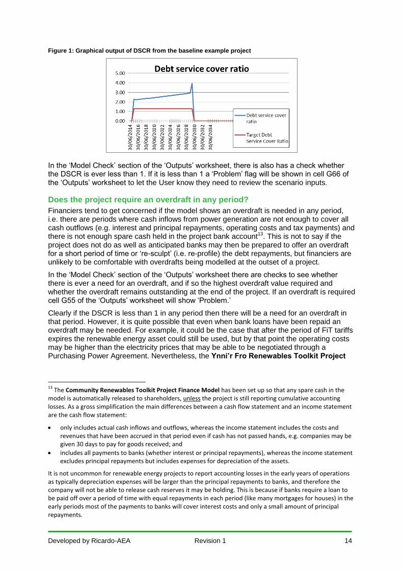
With a defined value Users should look at the DSCR graph to see if the DSCR is above the target DSCR value. If it is not above the target value in all periods it is still possible that a bank may be prepared to lend to a project so long as the average DSCR is above the target value and the DSCR is only below the target value in a few periods. To accept this, banks may agree to ‘sculpt’ the repayment profile, which means changing the repayment profile. It is even possible banks may agree to sculpt the repayment profile (or offer a smaller loan) if the average DSCR is below the target value. The DSCR in the Ynni’r Fro Renewables Toolkit Project Finance Model is shown in Figure 1. The baseline is a P50 scenario which is showing the average annual energy yield predicted for a project, i.e. the annual energy output that is most likely to occur in an ‘average’ year. The example is based on a hypothetical 200kW wind project, with an estimated 788.4MWh annual output and an old 18.4 p/kWh Feed-in-Tariff (FiT) rate. It assumes shareholders contribute £193,213 and a bank lends £608,273.12 The project operation costs are assumed to be £19,500 per year at the start of operations, development costs of £76,000 spread over 6 months and construction costs of £662,000 spread over 12 months.

12

Note that the model default is that 75% of costs are financed by debt and 25% by equity. However, this is before interest incurred in the construction phase is added to the total loan amount, which explains why at the end of the construction phase the ratio of debt to equity is slightly different at 75.9% : 24.1%.


Figure 1: Graphical output of DSCR from the baseline example project

In the ‘Model Check’ section of the ‘Outputs’ worksheet, there is also has a check whether the DSCR is ever less than 1. If it is less than 1 a ‘Problem’ flag will be shown in cell G66 of the ‘Outputs’ worksheet to let the User know they need to review the scenario inputs.

Does the project require an overdraft in any period?

Financiers tend to get concerned if the model shows an overdraft is needed in any period, i.e. there are periods where cash inflows from power generation are not enough to cover all cash outflows (e.g. interest and principal repayments, operating costs and tax payments) and there is not enough spare cash held in the project bank account13. This is not to say if the project does not do as well as anticipated banks may then be prepared to offer an overdraft for a short period of time or ‘re-sculpt’ (i.e. re-profile) the debt repayments, but financiers are unlikely to be comfortable with overdrafts being modelled at the outset of a project.

In the ‘Model Check’ section of the ‘Outputs’ worksheet there are checks to see whether there is ever a need for an overdraft, and if so the highest overdraft value required and whether the overdraft remains outstanding at the end of the project. If an overdraft is required cell G55 of the ‘Outputs’ worksheet will show ‘Problem.’

Clearly if the DSCR is less than 1 in any period then there will be a need for an overdraft in that period. However, it is quite possible that even when bank loans have been repaid an overdraft may be needed. For example, it could be the case that after the period of FiT tariffs expires the renewable energy asset could still be used, but by that point the operating costs may be higher than the electricity prices that may be able to be negotiated through a Purchasing Power Agreement. Nevertheless, the Ynni’r Fro Renewables Toolkit Project

13

The Community Renewables Toolkit Project Finance Model has been set up so that any spare cash in the model is automatically released to shareholders, unless the project is still reporting cumulative accounting losses. As a gross simplification the main differences between a cash flow statement and an income statement are the cash flow statement:

only includes actual cash inflows and outflows, whereas the income statement includes the costs and revenues that have been accrued in that period even if cash has not passed hands, e.g. companies may be given 30 days to pay for goods received; and

includes all payments to banks (whether interest or principal repayments), whereas the income statement excludes principal repayments but includes expenses for depreciation of the assets.

It is not uncommon for renewable energy projects to report accounting losses in the early years of operations as typically depreciation expenses will be larger than the principal repayments to banks, and therefore the company will not be able to release cash reserves it may be holding. This is because if banks require a loan to be paid off over a period of time with equal repayments in each period (like many mortgages for houses) in the early periods most of the payments to banks will cover interest costs and only a small amount of principal repayments.


Finance Model has been structured with the default assumption that the asset life of the renewable energy asset is the same as the FiT tariff period.

What is the equity return?

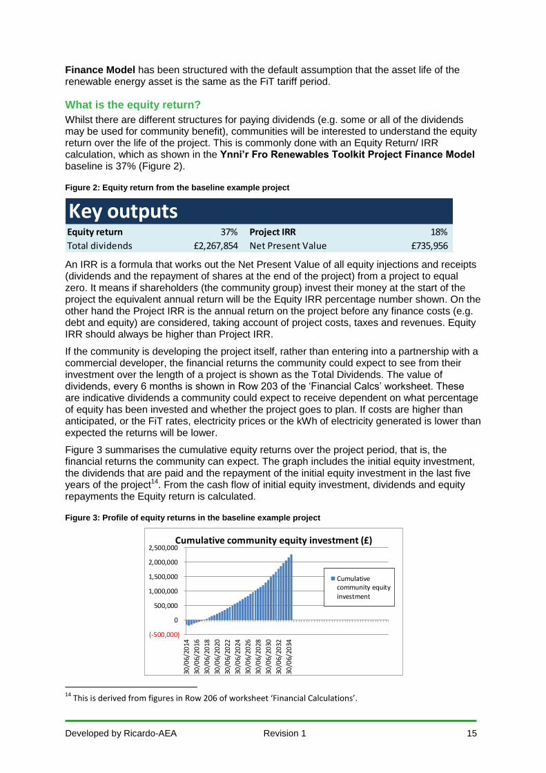
Whilst there are different structures for paying dividends (e.g. some or all of the dividends may be used for community benefit), communities will be interested to understand the equity return over the life of the project. This is commonly done with an Equity Return/ IRR calculation, which as shown in the Ynni’r Fro Renewables Toolkit Project Finance Model baseline is 37% (Figure 2).

Figure 2: Equity return from the baseline example project

An IRR is a formula that works out the Net Present Value of all equity injections and receipts (dividends and the repayment of shares at the end of the project) from a project to equal zero. It means if shareholders (the community group) invest their money at the start of the project the equivalent annual return will be the Equity IRR percentage number shown. On the other hand the Project IRR is the annual return on the project before any finance costs (e.g. debt and equity) are considered, taking account of project costs, taxes and revenues. Equity IRR should always be higher than Project IRR.

If the community is developing the project itself, rather than entering into a partnership with a commercial developer, the financial returns the community could expect to see from their investment over the length of a project is shown as the Total Dividends. The value of dividends, every 6 months is shown in Row 203 of the ‘Financial Calcs’ worksheet. These are indicative dividends a community could expect to receive dependent on what percentage of equity has been invested and whether the project goes to plan. If costs are higher than anticipated, or the FiT rates, electricity prices or the kWh of electricity generated is lower than expected the returns will be lower.

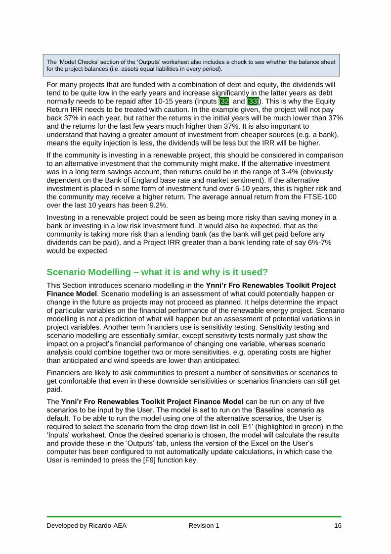
Figure 3 summarises the cumulative equity returns over the project period, that is, the financial returns the community can expect. The graph includes the initial equity investment, the dividends that are paid and the repayment of the initial equity investment in the last five years of the project14. From the cash flow of initial equity investment, dividends and equity repayments the Equity return is calculated.

Figure 3: Profile of equity returns in the baseline example project

14

This is derived from figures in Row 206 of worksheet ‘Financial Calculations’.

Equity return 37% Project IRR 18%

Total dividends £2,267,854 Net Present Value £735,956

Key outputs

(-500,000)

0

500,000

1,000,000

1,500,000

2,000,000

2,500,000

30/0

6/20

14

30/0

6/20

16

30/0

6/20

18

30/0

6/20

20

30/0

6/20

22

30/0

6/20

24

30/0

6/20

26

30/0

6/20

28

30/0

6/20

30

30/0

6/20

32

30/0

6/20

34

Cumulative community equity investment (£)

Cumulativecommunity equityinvestment


The ‘Model Checks’ section of the ‘Outputs’ worksheet also includes a check to see whether the balance sheet for the project balances (i.e. assets equal liabilities in every period).

For many projects that are funded with a combination of debt and equity, the dividends will tend to be quite low in the early years and increase significantly in the latter years as debt normally needs to be repaid after 10-15 years (Inputs [32] and [33]). This is why the Equity Return IRR needs to be treated with caution. In the example given, the project will not pay back 37% in each year, but rather the returns in the initial years will be much lower than 37% and the returns for the last few years much higher than 37%. It is also important to understand that having a greater amount of investment from cheaper sources (e.g. a bank), means the equity injection is less, the dividends will be less but the IRR will be higher.

If the community is investing in a renewable project, this should be considered in comparison to an alternative investment that the community might make. If the alternative investment was in a long term savings account, then returns could be in the range of 3-4% (obviously dependent on the Bank of England base rate and market sentiment). If the alternative investment is placed in some form of investment fund over 5-10 years, this is higher risk and the community may receive a higher return. The average annual return from the FTSE-100 over the last 10 years has been 9.2%.

Investing in a renewable project could be seen as being more risky than saving money in a bank or investing in a low risk investment fund. It would also be expected, that as the community is taking more risk than a lending bank (as the bank will get paid before any dividends can be paid), and a Project IRR greater than a bank lending rate of say 6%-7% would be expected.

Scenario Modelling – what it is and why is it used?

This Section introduces scenario modelling in the Ynni’r Fro Renewables Toolkit Project Finance Model. Scenario modelling is an assessment of what could potentially happen or change in the future as projects may not proceed as planned. It helps determine the impact of particular variables on the financial performance of the renewable energy project. Scenario modelling is not a prediction of what will happen but an assessment of potential variations in project variables. Another term financiers use is sensitivity testing. Sensitivity testing and scenario modelling are essentially similar, except sensitivity tests normally just show the impact on a project’s financial performance of changing one variable, whereas scenario analysis could combine together two or more sensitivities, e.g. operating costs are higher than anticipated and wind speeds are lower than anticipated.

Financiers are likely to ask communities to present a number of sensitivities or scenarios to get comfortable that even in these downside sensitivities or scenarios financiers can still get paid.

The Ynni’r Fro Renewables Toolkit Project Finance Model can be run on any of five scenarios to be input by the User. The model is set to run on the ‘Baseline’ scenario as default. To be able to run the model using one of the alternative scenarios, the User is required to select the scenario from the drop down list in cell ‘E1’ (highlighted in green) in the ‘Inputs’ worksheet. Once the desired scenario is chosen, the model will calculate the results and provide these in the ‘Outputs’ tab, unless the version of the Excel on the User’s computer has been configured to not automatically update calculations, in which case the User is reminded to press the [F9] function key.


Example of Scenario modelling with the Ynni’r Fro Renewables Toolkit Project Finance Model

Figure 4 provides a screenshot of some of the cells in the Ynni’r Fro Renewables Toolkit Project Finance Model (covered in Section 3). To this four other scenarios have been added, by copying exactly the same numbers as in the Baseline Column G in the ‘Inputs’ worksheet into columns H, I and J, and then changing some of the numbers. The four scenarios are:

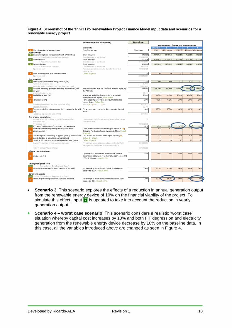
Scenario 1: This scenario illustrates the effects of capital costs being 10% higher than the baseline assumption. The way to reflect this in the model is by updating input variable [19] shown in the blue circle in Figure 4 from 100% to 110%.

However, Users should note that if they want to show a sensitivity where the profile of the construction costs changes (or the construction period becomes shorter or longer) they will need to change the numbers in the ‘Construction Costs’ worksheet. After doing this all scenarios will show this revised profile. Therefore, Users should save different versions of the model if they want to change profiles and timings of construction costs, but input variable [19] allows for simple uniform changes.

Scenario 2: This scenario considers a reduction, or degression of the Feed-in-Tariff, by 10% before FiT contracts can be signed. This is achieved by altering the input variable [11].

FIT levels are subject to regular review and, as of 1 April 2014, the Government is using an approach called ‘contingent degression’ to calculate what the reduction in the FiT rate should be. It is based on the generation capacity of installations pre-accredited and registered for the FiT for each technology the each tariff in the preceding time period.

The level of degression can be from 2.5% to 20%, with a standard reduction of 5%. For example, if a buoyant market for wind projects below 100kW results in 13.1MW of installed capacity or more pre-accredited and registered, this will trigger a 20% reduction in future FiT levels for new wind projects below 100kW in the following period.

For more information on the non-PV degression thresholds, please refer to the Monthly MCS and ROOFIT degression statistics dataset. This dataset provides up to date monthly data on accredited installation on the Microgeneration Certification Scheme (MCS) Installation Database and installations with a total installed capacity accredited through the ROO-FIT scheme.15 The dataset provides the thresholds for solar PV and non-solar PV installations as well as the degression applicable to technologies due to installed capacity meeting these thresholds.

15

The MCS database (http://www.microgenerationcertification.org/about-us/about-us) registers microgeneration products producing electricity (up to 50kW) and heat (up to 45kW) from renewable sources whilst the ROO-FIT scheme (https://www.ofgem.gov.uk/environmental-programmes/feed-tariff-fit-scheme/applying-feed-tariff/roo-fit) accredits solar PV and wind installations that have a declared net capacity greater than 50kW and up to and including 5MW and all anaerobic digestion and hydro installations up to and including 5MW.

https://www.gov.uk/government/statistical-data-sets/monthly-mcs-and-roofit-statistics

https://www.gov.uk/government/statistical-data-sets/monthly-mcs-and-roofit-statistics

http://www.microgenerationcertification.org/about-us/about-us

https://www.ofgem.gov.uk/environmental-programmes/feed-tariff-fit-scheme/applying-feed-tariff/roo-fit

https://www.ofgem.gov.uk/environmental-programmes/feed-tariff-fit-scheme/applying-feed-tariff/roo-fit


Figure 4: Screenshot of the Ynni’r Fro Renewables Project Finance Model input data and scenarios for a renewable energy project

Scenario 3: This scenario explores the effects of a reduction in annual generation output from the renewable energy device of 10% on the financial viability of the project. To simulate this effect, input [7] is updated to take into account the reduction in yearly generation output.

Scenario 4 – worst case scenario: This scenario considers a realistic ‘worst case’ situation whereby capital cost increases by 10% and both FiT degression and electricity generation from the renewable energy device decrease by 10% on the baseline data. In this case, all the variables introduced above are changed as seen in Figure 4.

Scenario choice (dropdown) Baseline

<--------------- Scenarios ---------------->Comments Baseline 1 2 3 4

1 Short description of scenario basis Free-flow text box Worst case P50 +10% capex -10% FiT -10% gen Worst case

Project timings

2 Development phase start (potentially with CARES loan) Enter mm/yyyy 08/2013 08/2013 08/2013 08/2013 08/2013 08/2013

---------> Actual development phase start date Calculates end of month date 31/08/2013

3 Financial close Enter mm/yyyy 01/2014 01/2014 01/2014 01/2014 01/2014 01/2014

---------> Actual financial close date Calculates end of month date 31/01/2014

4 Construction end Enter mm/yyyy 12/2014 12/2014 12/2014 12/2014 12/2014 12/2014

---------> Actual construction end Calculates end of month date 31/12/2014

Operations start Assumes operations start the day after the end of

construction

01/01/2015

5 Asset lifespan (years from operations start) Default 20 years 20 20 20 20 20 20

Operations end 31/12/2034

Energy output

6 Rated power of renewable energy device (kW) 300 300 300 300 300 300

Number of hours in a year 8,760

Maximum power production per year (kWh per year) 2,628,000

7Maximum electricity generated assuming no downtime (kWh

per year)

This value comes from the Technical Advisers report, eg.

the P90 value

709,560 788,400 788,400 788,400 709,560 709,560

Implied utilisation of plant 27.0%

8Availability of plant (%) Warranted availability from supplier to account for

maintenance and repairs. Default 95%

95.0% 95.0% 95.0% 95.0% 95.0% 95.0%

9Parasitic load (%) Percentage of power that is used by the renewable

energy device. Default 0%

0.0% 0.0% 0.0% 0.0% 0.0% 0.0%

Available power output per year (kWh per year) This is [7] * [8]% * (1 - [9]%) 674,082

Capacity factor (%) 25.7%

10Percentage of electricity generated that is exported to the grid

(%)

Some power may be used by the community. Default

100%

100% 100% 100% 100% 100% 100%

Electricity exported per year (kWh) 674,082

Energy price assumptions

Number of months to obtain signed FiT contract after

operations start

It is assumed the FiT contract is pre-accredited before

operations start

0

FiT contract start 01/01/2015

11 FiT rate (p/kWh) at date of operations commencement 16.56 18.4 18.4 16.56 18.4 16.56

12

Electricity export tariff (p/kWh) at date of operations

commencement

Price for electricity exported to the grid (shown in [10])

through a Purchasing Power Agreement (PPA). Default

4.5p/kWh.

4.5 4.5 4.5 4.5 4.5 4.5

13Levy Exemption Certificate (LEC) price (p/kWh) for electricity

exported at date of operations commencement

LEC price if not included within export price in [12].

Default 0.4 p/kWh.

0.4 0.4 0.4 0.4 0.4 0.4

14 Length of FiT contract from date of operations start (years) Default 20 years. 20 20 20 20 20 20

Signed FiT contract in April-March price basis FiT contract prices adjust by inflation on the 1st April

each year as do all other inflation assumptions

01/04/2014

First FiT annual inflation change 01/04/2015

Inflation rate assumptions

15 Inflation rate (%)

Operating cost inflation rate with the same inflation

assumptions applying to FiT, electricity export prices and

LECs (if relevant). Default 2.5%.

2.5% 2.5% 2.5% 2.5% 2.5% 2.5%

Development phase costs

16 -----> See worksheet 'Development Costs'

17Sensitivity (percentage of developments cost modelled) For example to model a 5% increase in development

costs enter 105%. Default 100%.

100% 100% 100% 100% 100% 100%

Construction costs

18 -----> See worksheet 'Construction Costs'

19Sensitivity (percentage of construction cost modelled) For example to model a 5% decrease in construction

costs enter 95%. Default 100%.

110% 100% 110% 100% 100% 110%


Results of scenario modelling with the Ynni’r Fro Renewables Toolkit Project Finance Model

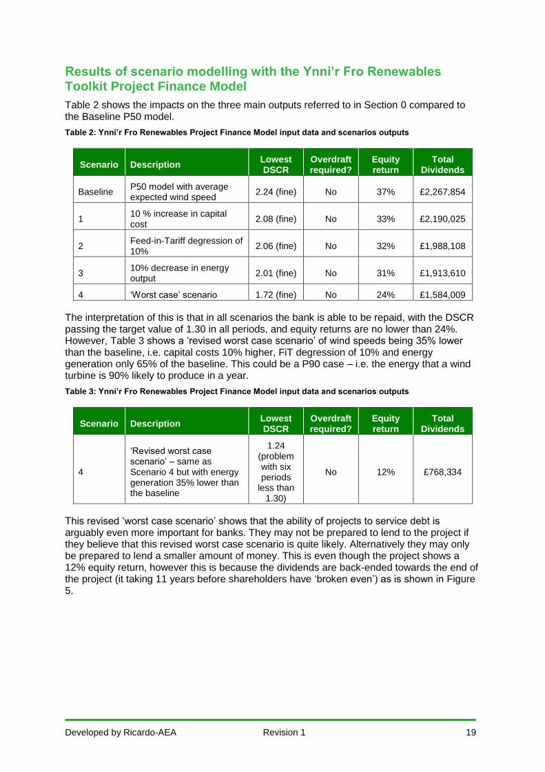
Table 2 shows the impacts on the three main outputs referred to in Section 0 compared to the Baseline P50 model.

Table 2: Ynni’r Fro Renewables Project Finance Model input data and scenarios outputs

Scenario Description Lowest DSCR

Overdraft required?

Equity return

Total Dividends

Baseline P50 model with average expected wind speed

2.24 (fine) No 37% £2,267,854

1 10 % increase in capital cost

2.08 (fine) No 33% £2,190,025

2 Feed-in-Tariff degression of 10%

2.06 (fine) No 32% £1,988,108

3 10% decrease in energy output

2.01 (fine) No 31% £1,913,610

4 ‘Worst case’ scenario 1.72 (fine) No 24% £1,584,009

The interpretation of this is that in all scenarios the bank is able to be repaid, with the DSCR passing the target value of 1.30 in all periods, and equity returns are no lower than 24%. However, Table 3 shows a ‘revised worst case scenario’ of wind speeds being 35% lower than the baseline, i.e. capital costs 10% higher, FiT degression of 10% and energy generation only 65% of the baseline. This could be a P90 case – i.e. the energy that a wind turbine is 90% likely to produce in a year.

Table 3: Ynni’r Fro Renewables Project Finance Model input data and scenarios outputs

Scenario Description Lowest DSCR

Overdraft required?

Equity return

Total Dividends

4

‘Revised worst case scenario’ – same as Scenario 4 but with energy generation 35% lower than the baseline

1.24 (problem with six periods

less than 1.30)

No 12% £768,334

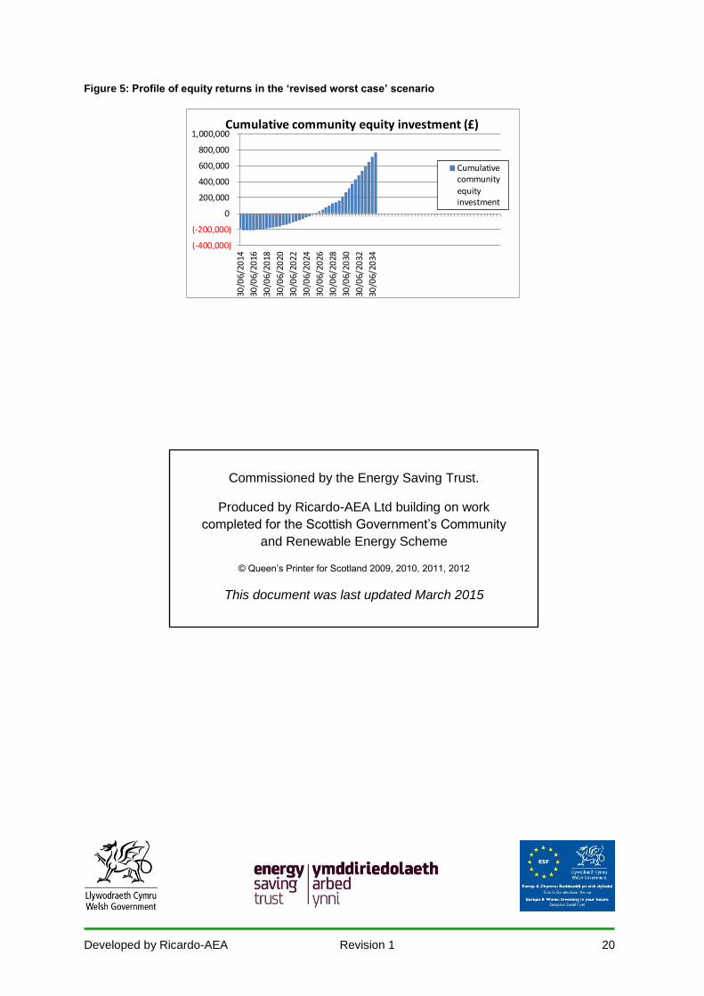
This revised ‘worst case scenario’ shows that the ability of projects to service debt is arguably even more important for banks. They may not be prepared to lend to the project if they believe that this revised worst case scenario is quite likely. Alternatively they may only be prepared to lend a smaller amount of money. This is even though the project shows a 12% equity return, however this is because the dividends are back-ended towards the end of the project (it taking 11 years before shareholders have ‘broken even’) as is shown in Figure 5.


Figure 5: Profile of equity returns in the ‘revised worst case’ scenario

(-400,000)

(-200,000)

0

200,000

400,000

600,000

800,000

1,000,000

30/0

6/20

14

30/0

6/20

16

30/0

6/20

18

30/0

6/20

20

30/0

6/20

22

30/0

6/20

24

30/0

6/20

26

30/0

6/20

28

30/0

6/20

30

30/0

6/20

32

30/0

6/20

34

Cumulative community equity investment (£)

Cumulativecommunityequityinvestment

Commissioned by the Energy Saving Trust.

Produced by Ricardo-AEA Ltd building on work

completed for the Scottish Government’s Community

and Renewable Energy Scheme

© Queen’s Printer for Scotland 2009, 2010, 2011, 2012

This document was last updated March 2015

finance model guide - energy saving trust · finance model guide ... ‘construction costs’...

Documents