1

Independent Component Analysis Techniques for Source

Separation

Sumanapala D.R. (E/10/347)

Sumanapala D.R. (E/10/348)

Thushan S. (E/10/361)

Supervised by,

Dr. Godaliyadda G.M.R.I.

Dr. Suraweera S.A.H.A.

Dr. Wijayakulasooriya J.V.

Group 15

i

Abstract

Utilization of Blind Source Separation (BSS) techniques to extract and interpret

data from various types of multi-sensory systems is recognized as a highly

demanding area of modern day research and studies. The significance is that, BSS

techniques do not rely on the information related to the source signals which are

totally unknown and yet to be extracted. Further, the sensor measurements are

always noisy in practice making this a noise reduction problem coupled with a

source separation problem. And also, most source signals in a noisy mixture have

overlapping bandwidths making it impossible to use standard filtering techniques

to separate the sources. In our project, we show that the Independent Component

Analysis (ICA) [1, 2] based adaptive method can be used to overcome this problem

to extract source signals effectively from a given over-determined source signal

mixture.

Due to the fact that ICA utilizes higher order statistics such as mutual

independence, kurtosis, entropy etc., it has the capacity to extract sources with

overlapping spectral contents as well.

This blind source separation (BSS) technique we propose can be applicable to a wide

array of applications including but not limited to acoustics, communication, context

aware networks, computer vision, defense and security systems and bio-medicine.

We have analyzed a brute force approach for source separation through the

identification of local maxima points for the mixtures. Due to its limitations in

higher dimensions, a gradient based adaptive approach was proposed. The

adaptation process attempts to converge to a local maximum (in the super Gaussian

case) through a gradient ascent approach.

We conducted a detailed analysis of the kurtosis based gradient ascent ICA

algorithm in the weight vector normalized subspace and the adaptation path and

the variation of the weight vector are depicted. This enabled us to understand the

behavior of the kurtosis surface gradient in the reduced space and realize its

limitations as a convergence criterion. Thus, a method based on stability of the

ii

weight vector was proposed as the convergence criterion for the adaptation process.

The proposed adaptation method was extended for sub Gaussian and super-sub

Gaussian mixtures as well.

Later we explored the complex valued ICA [3, 4] for the blind source separation

from complex valued mixtures which involves complex valued kurtosis. This method

was more accurate and fast compared to the real valued algorithm. Further, the

complex valued algorithm was improved to a frequency domain algorithm [5] which

can be effectively used to extract sources from non-linearly mixed source signals.

The implemented algorithms were used for different applications including acoustic

source extraction and image restoration problems to get a solid verification and to

mark the significance of ICA based BSS methods.

iii

Acknowledgements

We would like to gratefully acknowledge the supportive and enthusiastic

supervision by Dr. G.M.R.I. Godaliyadda, Dr. J.V. Wijayakulasooriya, Dr. S.A.H.A.

Suraweera and Dr. M.P.B. Ekanayake. Their vision, comments and the cooperation

helped us to take our project really high. The guidance, encouragement,

enlightenment and the cooperation they made in the course of this project have

been invaluable for us. None of this will be successful without their immense help

they made by sacrificing hours of their valuable time to discuss matters, solutions

and improvements that we had to make during the time of this undergraduate

project.

And also we hereby thank Prof. J.B. Ekanayake, Head of the Department of

Electrical and Electronic Engineering, University of Peradeniya, for his cooperation

as the subject coordinator of EE548.

Instructors and all the other staff members of the department of electrical and

electronic engineering who supported us in many ways should be thanked here as

well.

Last but not least, we wish to thank all our friends and colleagues who always

encouraged and helped us one way or the other to make our project even more

successful.

iv

Contents

Chapter 1: Introduction ............................................................................................ 1

1.1 Overview ............................................................................................................... 1

1.2 Objective ................................................................................................................ 4

1.3 Signals used for the preliminary study ............................................................... 5

Chapter 2: Independent Component Analysis and Strategies for Blind

Source Separation ...................................................................................................... 6

2.1 Introduction .......................................................................................................... 6

2.2 Mathematical representation of signals .............................................................. 7

2.3 Comparing Signal mixtures and sources graphically. ........................................ 8

2.3.1 Using the Scatter Plot .................................................................................... 8

2.3.2 Using the Histogram ...................................................................................... 8

2.4 Mixing of signals ................................................................................................... 9

2.5 Un-mixing of signals ........................................................................................... 10

Chapter 3: Kurtosis Based Blind Source Separation through the Brute

Force approach ......................................................................................................... 12

3.1 Introduction ........................................................................................................ 12

3.2 Mathematical model ........................................................................................... 14

3.2.1 Dimension Reduction Process ...................................................................... 14

3.2.2 Unmixing Process ......................................................................................... 17

3.2.3 Un-mixing sources from a mixture of four signals ...................................... 18

3.3 Conclusions: Limitations for the Brute force method ....................................... 21

Chapter 4: Source Extraction by Gradient based Algorithms........................ 23

4.1 Introduction ........................................................................................................ 23

4.2 The convergence criteria ................................................................................... 26

4.2.1 Minimum gradient ........................................................................................ 26

4.2.2 Minimum kurtosis difference between two adjacent points ....................... 26

4.2.3 Checking the stability of the weight vector ................................................. 27

4.3 Preliminary work ................................................................................................ 27

4.3.1 Gradient Ascent: Un-mixing a super Gaussian source signal .................... 28

4.3.2 Gradient Descent: Un-mixing a sub Gaussian source signal ..................... 29

4.4 Results and conclusions ...................................................................................... 31

v

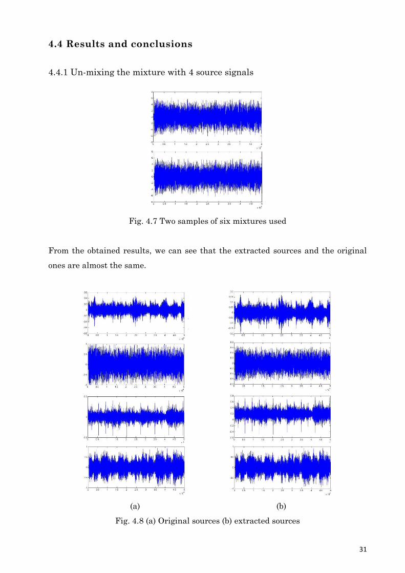
4.4.1 Un-mixing the mixture with 4 source signals ............................................. 31

Chapter 5: Extension of ICA for Complex Valued Mixtures ........................... 33

5.1 Complex kurtosis and its gradient ..................................................................... 33

5.2 Gradient of Kurtosis ........................................................................................... 33

5.2.1 Definition: Wirtinger Differential Operator ................................................ 34

5.3 Update equation ................................................................................................. 36

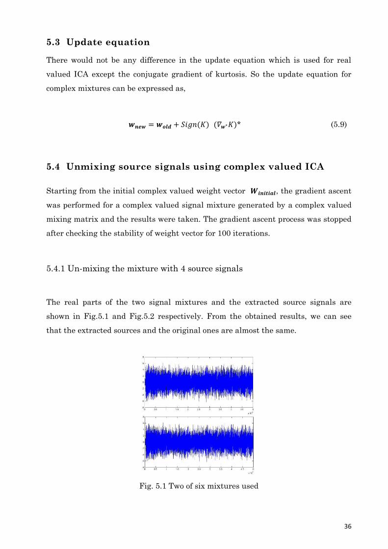
5.4 Unmixing source signals using complex valued ICA ....................................... 36

5.4.1 Un-mixing the mixture with 4 source signals ............................................. 36

Chapter 6: Frequency domain ICA for source extraction in frequency

domain ........................................................................................................................ 38

6.1 Unmixing source signals using frequency domain ICA .................................... 38

6.1.1 Un-mixing the mixture with 4 source signals ............................................. 39

Chapter 7: Application of ICA for acoustic signal mixtures ........................... 40

7.1 Possible applications ........................................................................................... 40

7.2 Extracting sources from linear acoustic signal mixtures .................................. 40

7.2.1 Results ........................................................................................................... 40

7.2.2 Performance of three algorithms for linear acoustic signal mixtures ........ 41

7.3 Extracting sources from non-linear acoustic signal mixtures .......................... 42

7.3.1 Process of extraction ..................................................................................... 42

Chapter 8: Application of ICA for extracting sources from image mixtures

...................................................................................................................................... 45

8.1 Application of ICA techniques for image mixtures ........................................... 45

8.2 Image inverting problem ................................................................................... 46

8.3 Applying ICA to linear image mixtures ............................................................. 48

8.4 Removing reflections using this concept ............................................................ 50

8.5 Extracting sources from non-linear image mixtures ......................................... 51

8.6 Extracting background using frequency domain ICA ....................................... 53

8.7 Conclusion .......................................................................................................... 54

Chapter 9: Enhancing images using complex valued ICA ............................... 56

9.1 Image enhancement process and results comparison ..................................... 56

9.2 Selecting the best equalized image ................................................................... 59

9.3 Conclusions ......................................................................................................... 60

Chapter 10: Conclusions ......................................................................................... 61

References .................................................................................................................. 63

vi

vii

List of figures

Fig. 1. 1 Histograms (a) for one source, (b) for two sources (c) for three source 3

Fig. 1. 2 Application of Blind Source Separation 4

Fig. 1.3 Four acoustic source signals used 5

Fig. 2.1 (a) Scatter plot for two mixtures. (b) Scatter plot for two source signals 8

Fig. 2.2 (a) Histogram for a source signal (b) Histogram for a mixture of 4

sources 8

Fig. 2.3 The basic model for the blind source separation process based on ICA 11

Fig. 3.1 Reduced space for two signal mixtures 13

Fig. 3.2 Variance distribution of the principal components 15

Fig. 3.3 Logarithmic variance distribution of the principal components 16

Fig. 3.4 Variance distribution of logarithmic signal power of the first n

Principal components 16

Fig. 3.5 Derivative of variance distribution of logarithmic signal power of

the first n principal components 16

Fig. 3.6 Original sources 18

Fig. 3.7 Two of six sample mixtures 18

Fig. 3.8 Polar plot for the kurtosis variance of last two source mixtures 18

Fig. 3.9 Extracted source signals 19

Fig. 3.10 Comparison of the original sources and the extracted ones 20

Fig. 3.11 Kurtosis variation for a three source case 21

Fig. 4.1 Reaching the maximum kurtosis by the gradient ascent 27

Fig. 4.2 Kurtosis variation for the gradient ascent 27

Fig. 4.3 Variation of first component of the weight vector for the

gradient ascent 28

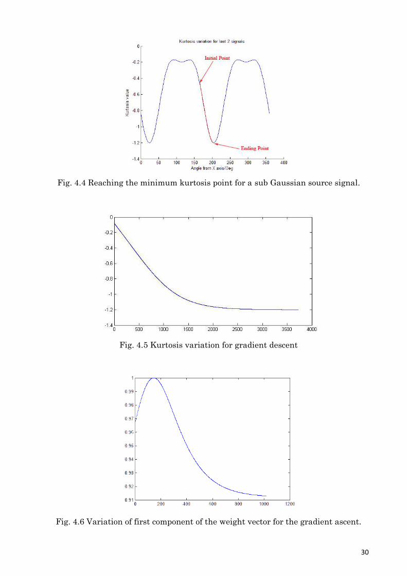
Fig. 4.4 Reaching the minimum kurtosis point for a sub Gaussian source signal 29

Fig. 4.5 Kurtosis variation for gradient descent 29

viii

Fig. 4.6 Variation of first component of the weight vector for the

gradient ascent 29

Fig. 4.7 Two samples of six mixtures used 30

Fig. 4.8 (a) Original sources (b) extracted sources 30

Fig. 5.1 Two of six mixtures used 35

Fig. 5.2 (a) Original sources (b) extracted sources using complex valued ICA 36

Fig. 6.1 Two of six mixtures used 38

Fig. 6.2 (a) Original sources (b) extracted sources using frequency domain ICA 38

Fig. 7.1 (a) Original sources, extracted sources using (b) real valued ICA,

(c) complex valued ICA, (d) frequency domain ICA 40

Fig. 7.2 Original source signal 42

Fig. 7.3 Three samples of eight distorted acoustic signals 42

Fig. 7.4 Sample of extracted sources using time domain complex

Valued algorithm 43

Fig. 7.5 Extracted source using frequency domain complex valued algorithm 43

Fig. 8.1 Converting image to a signal 45

Fig. 8.2 Unwrapped signal of a (a) un-inverted image (b) inverted image 46

Fig. 8.3 Source images used for generating the mixtures 47

Fig. 8.4 Four samples of the image mixtures 47

Fig. 8.5 Extracted sources for real valued ICA with ŋ = 0.1 and Stabilizing w

for 5 decimal points 48

Fig. 8.6 Extracted sources for complex valued time domain ICA with ŋ = 1 and

stabilizing w for 4 decimal points 48

Fig. 8.7 Extracted sources for complex valued frequency domain ICA

With ŋ = 1 and stabilizing w for 4 decimal points 48

Fig. 8.8 Sample images with two different levels of reflections 49

Fig. 8.9 (a) Extracted background, (b) extracted refection part 49

Fig. 8.10 (a) Source images (b) extracted sources from the time domain complex

valued ICA (c) extracted sources from the frequency domain complex

valued ICA 51

ix

Fig. 8.11 (a) Extracted background image from complex valued time domain ICA

(b) Extracted background image from the frequency domain Complex

valued ICA 51

Fig. 8.12 Three samples of the 10 occluded source images 53

Fig. 8.13 Extracted image using time domain complex valued ICA algorithm 53

Fig. 8.14 Extracted image using frequency domain complex valued

ICA algorithm 53

Fig. 9.1 Original image used for equalization 56

Fig. 9.2 (a) Red component of the image (b) Green component of the image (c) Blue

component of the image 56

Fig. 9.3 Extracted images from RGB components using complex ICA algorithm 56

Fig. 9.4 RGB images obtained by replacing value component of HSV image with the

extracted independent components (a), (b), (c) separately 56

Fig. 9.5 Image obtained by averaging RGB components of the original image 57

Fig. 9.6 RGB image obtained by replacing value component of the HSV

representation of the image 57

Fig. 9.7 Results obtained for frequency domain ICA 58

Fig. 9.8 Waveforms of the images when they are ordered according to variance in

descending order with (a) largest, (b) second largest and (c) smallest variance

waveform 59

Fig. 9.9 Images corresponding to (a), (b) and (c) of Fig.9.8 59

1

Chapter 1

Introduction

1.1 Overview

In today’s world, information plays a vital role. Day by day, the ability to access

data is improving and many problems arise when we try to extract out only the

important information from a given collection of data. Most often, that collection of

data can be too noisy or it can be originated from a mixture of unknown sources. If

the information comes in the form of signals, it would be a problem of extracting

source signals from a set of noisy signals mixtures. The process of extracting those

unknown source signals is called Blind Source Separation (BSS). [1] As the name

implies, BSS methods do not rely on the information related to the source signals

which are to be extracted. Generally, the number of mixtures is kept higher than

the possible number of sources to be extracted. In that case, the problem is said to

be over-determined.

In this project, our target is to introduce a reliable BSS method based on

Independent component Analysis (ICA) to extract sources from over-determined

signal mixtures. And also with our algorithms, we are trying to make that

extraction process faster and solid keeping the processing power at a lower level.

Also we associate some mathematical concepts such as Principal Component

Analysis (PCA) throughout the process. [6]

ICA is widely used in many applications including biomedical applications (ECG,

EEG [7], MRI and fMRI [8] etc.), face and speech recognition [9], finance, traffic

sensor systems and wireless communication.

A key concept that constitutes the foundation of independent component analysis is

statistical independence. To simplify the above statement, consider the case of two

different random variables s1 and s2. The random variable s1 is independent of s2,

if the information about the value of s1 does not provide any information about the

2

value of s2, and vice versa. Here, s1 and s2 could be random signals originating

from two different physical processes that are not related to each other.

In natural processes, basically the signal mixtures are formed by adding up each of

the independent source signals together by different proportions. This way, each

source can be assigned with some weightage. This weightage can be considered as a

mixing coefficient. By putting up those coefficients in to a matrix we get the mixing

matrix.[1] This kind of a mixing process is called a linear mixing process.

The sampled signals are written in the form of matrices or vectors. Their entries

form distributions that can be statistically analyzed, and in this project we compare

the statistical independency of the sources vs. mixtures. Statistical independence

associates with the Gaussianity of data points and the parameter kurtosis can give

a decent numerical value to measure how the sources are statistically independent

when the mixtures are not. The kurtosis can be calculated by the simple equation,

∑

∑

.

(1.1)

Source signals have their kurtosis values maximally higher (negatively or

positively) according to the nature of the signal. Gaussian signals have zero

kurtosis. Super-Gaussian signals have positive kurtosis value and it will be

negative for sub-Gaussian signals.[1]

When the source signals keep adding up mixing together by different proportions,

Gaussianity increases and the magnitude of the kurtosis becomes smaller. This

concept can be theoretically proved by the well-known central limit theorem and

also can be clearly observed by looking at the distributions of the related entries.

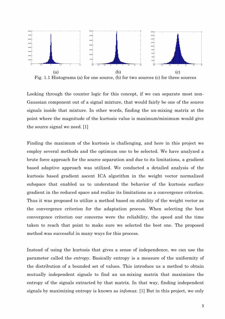
Fig.1.1 illustrates how the Gaussianity increases when more and more source

signals are added together.

3

(a) (b) (c)

Fig. 1.1 Histograms (a) for one source, (b) for two sources (c) for three sources

Looking through the counter logic for this concept, if we can separate most non-

Gaussian component out of a signal mixture, that would fairly be one of the source

signals inside that mixture. In other words, finding the un-mixing matrix at the

point where the magnitude of the kurtosis value is maximum/minimum would give

the source signal we need. [1]

Finding the maximum of the kurtosis is challenging, and here in this project we

employ several methods and the optimum one to be selected. We have analyzed a

brute force approach for the source separation and due to its limitations, a gradient

based adaptive approach was utilized. We conducted a detailed analysis of the

kurtosis based gradient ascent ICA algorithm in the weight vector normalized

subspace that enabled us to understand the behavior of the kurtosis surface

gradient in the reduced space and realize its limitations as a convergence criterion.

Thus it was proposed to utilize a method based on stability of the weight vector as

the convergence criterion for the adaptation process. When selecting the best

convergence criterion our concerns were the reliability, the speed and the time

taken to reach that point to make sure we selected the best one. The proposed

method was successful in many ways for this process.

Instead of using the kurtosis that gives a sense of independence, we can use the

parameter called the entropy. Basically entropy is a measure of the uniformity of

the distribution of a bounded set of values. This introduce us a method to obtain

mutually independent signals to find an un-mixing matrix that maximizes the

entropy of the signals extracted by that matrix. In that way, finding independent

signals by maximizing entropy is known as infomax. [1] But in this project, we only

-1 -0.5 0 0.5 1 1.50

1000

2000

3000

4000

5000

6000

7000

8000

-20 -15 -10 -5 0 5 10 15 200

500

1000

1500

2000

2500

3000

3500

-30 -20 -10 0 10 20 300

200

400

600

800

1000

1200

1400

1600

1800

4

focus on ICA based on kurtosis since it has many advantages compared with the

infomax approach. Unlike the kurtosis based method, infomax method can only

separate source signals from super-super Gaussian mixtures. It won’t work with the

sub-sub Gaussian and super-sub mixtures and that is a major drawback of that

method. On the other hand, infomax method is much complex. In this method,

matrix is bigger. That makes the related calculations computationally exhaustive.

Here we need to know the number of sources we have in the mixture which is

impractical in some cases. The other thing is, for infomax method, we need to use a

model pdf for sources and that would definitely add some errors. The good thing

about infomax is it extracts every source signal at once, so that no iterative process

to be followed. And also this process is pretty much systematic and orderly. After

considering all these aspects, it was easy to decide that kurtosis based method is

the most suitable method for our project.

1.2 Objective

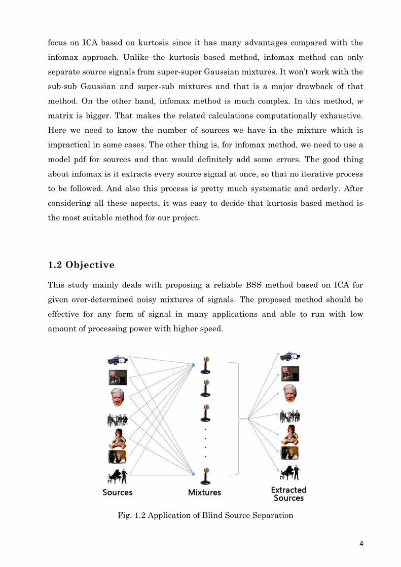
This study mainly deals with proposing a reliable BSS method based on ICA for

given over-determined noisy mixtures of signals. The proposed method should be

effective for any form of signal in many applications and able to run with low

amount of processing power with higher speed.

Fig. 1.2 Application of Blind Source Separation

5

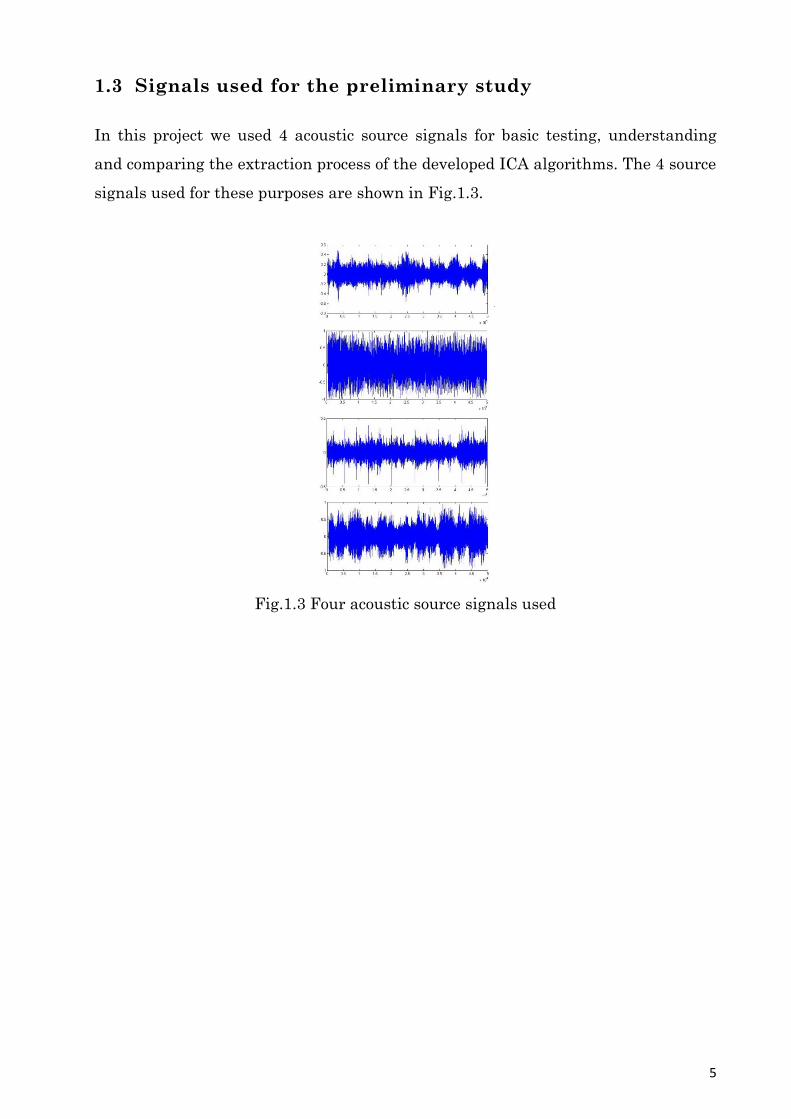
1.3 Signals used for the preliminary study

In this project we used 4 acoustic source signals for basic testing, understanding

and comparing the extraction process of the developed ICA algorithms. The 4 source

signals used for these purposes are shown in Fig.1.3.

Fig.1.3 Four acoustic source signals used

6

Chapter 2

Independent Component Analysis

and Strategies for Blind Source

Separation

2.1 Introduction

ICA has been applied in many fields related to signal processing which can be

diverse as speech processing, brain imaging (eg. fMRI [8] and Optical Imaging),

electrical brain systems (Eg. EEG signals) telecommunications and the stock

market prediction. [1]

ICA is based on simple, generic and physically realistic assumption that if different

signals are from different physical processes (natural or artificial), then those

signals are statistically independent. ICA takes advantage of the fact that the

implication of this assumption can be reversed, leading to a new assumption that is

proven to be practically true by numerous observations in practice. This new

assumption nicely points out that if statistically independent signals can be

extracted from signal mixtures, then these extracted signals must be from different

physical processes. Accordingly, ICA separates signal mixtures in to statistically

independent signals. If the assumptions of statistical independence is valid, then

each of the signals extracted by the independent component analysis should have

been generated by a different physical process, and therefore be a desired signal. [1]

As we discussed earlier, the mutual independence of the sources can be measured

using another parameter called the entropy. However same argument as it is

mentioned in the above paragraph can be adapted for the mutual independence.[1]

If the extracted signals have their entropy maximized, we can approximate that

they are very closer to the sources (that we need to extract) with a high certainty

level. This method is called the infomax.

7

ICA has its own model for the signals and the systems and the related operations

and calculations on them. The preceding content of this chapter represent those

facts.

2.2 Mathematical representation of signals

Mathematical representation of a sampled signal would be in matrix form as a row

vector.

S = (s1, s2, s3,…………, sn) (2.1)

This includes the amplitude values for each time step from 1 to n.

For “m” number of signals,

S1 = (

)

S2 = (

)

. . . . . . . . . . . . . . . . . . .

Sm = (

)

Including all the values of signals together in to one matrix having size of m×n,

(

)

For easiness of representation, we will take the ith column of this matrix as

Si = [

]T, so that the collection of signals would be the matrix S,

where S = [ S1 S2 S3 ………. Sn ].

8

2.3 Comparing Signal mixtures and sources graphically.

2.3.1 Using the Scatter Plot

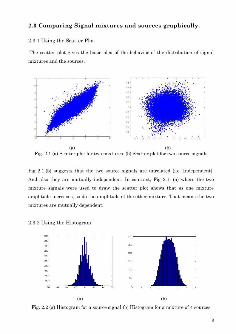
The scatter plot gives the basic idea of the behavior of the distribution of signal

mixtures and the sources.

(a) (b)

Fig. 2.1 (a) Scatter plot for two mixtures. (b) Scatter plot for two source signals

Fig 2.1.(b) suggests that the two source signals are unrelated (i.e. Independent).

And also they are mutually independent. In contrast, Fig 2.1. (a) where the two

mixture signals were used to draw the scatter plot shows that as one mixture

amplitude increases, so do the amplitude of the other mixture. That means the two

mixtures are mutually dependent.

2.3.2 Using the Histogram

(a) (b)

Fig. 2.2 (a) Histogram for a source signal (b) Histogram for a mixture of 4 sources

9

Fig. 2.2 shows that the histogram of any source signal is more non-Gaussian (i.e.

peaky) than the histogram of any signal mixture containing that source signal.

2.4 Mixing of signals

The fact that the outputs of the sensors compromise of some proportions of each

source signal presumably with some added noise, leads to the idea of mixing

coefficients. For a simple case of two signals mixing together, the following model is

proposed. [1]

We denote a signal mixture taken from a sensor we deploy as x1 and the two sources

are S1 and S2. And also the relative proportion of each signal is a and b. We specify

the magnitude of the mixture at the time t as .

= a×

+ b× (2.2)

If we consider x1, s1 and s2 over all n time indices then,

) = a ×

) + b ×

) (2.3)

This can be written more succinctly as,

x1 = a×s1 + b×s2 (2.4)

As we are concerned here un-mixing a set of two signal mixtures, a second mixture

can be given as,

x2 = c×s1 + d×s2 (2.5)

where the mixing coefficient c and d are different from a and b because the two

sensors mix the sources in a different manner.

10

If there are more sources we need same number of mixtures and this forms a

mixing matrix of the system. We denote it as .

A = (

) (2.6)

so that,

(

) (

) (

) (2.7)

or,

x = As (2.8)

It is possible to extend these equations in case of having any number of sources and

mixtures.

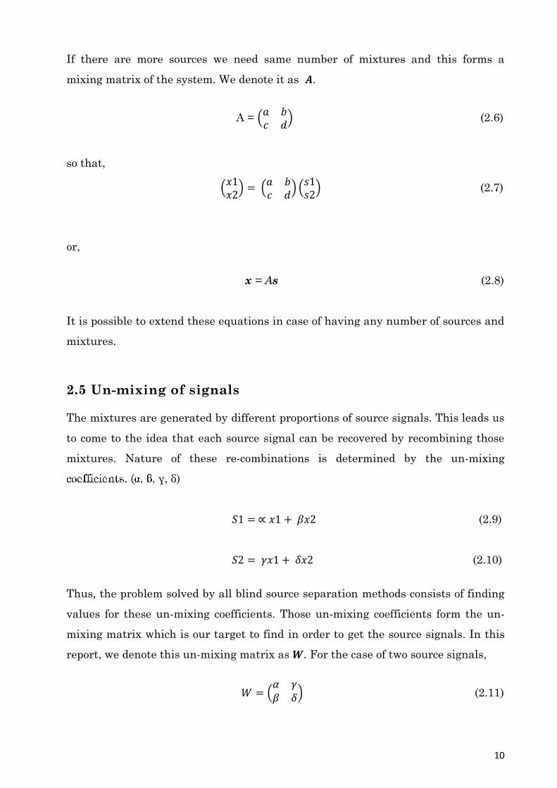
2.5 Un-mixing of signals

The mixtures are generated by different proportions of source signals. This leads us

to come to the idea that each source signal can be recovered by recombining those

mixtures. Nature of these re-combinations is determined by the un-mixing

γ, δ)

(2.9)

(2.10)

Thus, the problem solved by all blind source separation methods consists of finding

values for these un-mixing coefficients. Those un-mixing coefficients form the un-

mixing matrix which is our target to find in order to get the source signals. In this

report, we denote this un-mixing matrix as . For the case of two source signals,

( ) (2.11)

11

so that extraction of the signal represent in the mathematical sense, it would be,

(

) (

) (

) (2.12)

or,

s = x

(2.13)

Begining from an initial random un-mixing matrix, our aim is to tune up the matrix

until we get the source signals. In kurtosis based approach, we tune this for the

maximum kurtosis and in infomax we tune this for maximum entropy. [1] However,

both methods will extract some signals which can be effectively considered as

statistically independent sources.

Fig. 2.3 The basic model for the blind source separation process based on ICA

12

Chapter 3

Kurtosis Based Blind Source

Separation through the Brute

Force approach

3.1 Introduction

Brute force method is the simplest approach to find the un-mixing matrix where the

maximum or the minimum kurtosis occurs, and that point is to be tracked by

considering kurtosis values for all the weight vectors one by one. This is because

theoretically, each and every maxima or the minima should represent a source

signal which can be extracted. Here the maximum points will always extract out the

super Gaussian source signals and in case of the sub-Gaussian source signals, it

would be the minimum points. [1]

The Kurtosis can be calculated using the following equation. Here the kurtosis

plays a role as the measure of non-Gaussianity. Kurtosis can be expressed as,

∑

∑

(3.1)

It is known that the separated sources using ICA can be a scalar-multiplied version

of the original source signals. That means, there can always be a multiplication

factor and that would be a scalar quantity. This happens because the scalar

multiplication of the signal does not make any difference in its kurtosis value.

Therefore, all the weight vectors can be multiplied by different scalars. But their

direction keeps un-changed. Irrelevant of the magnitude, it is enough to know the

direction specified to proceed with the source extraction process. [1]

13

Therefore, it is only the direction of weight vector that matters for the ICA process,

because we don’t care how much the extracted sources are attenuated or amplified

compared to the original sources. We can later amplify or attenuate the extracted

sources depending on the requirement. Here, the problem is to somehow extract the

sources at any amplitude level. For our convenience, we extract the source signals

in the basis of having the un-mixing matrix , which has a unit modulus or a norm.

Note that in case of extracting one source signal, is a vector.

We keep = 1 for all randomly generated un-mixing matrices. Hence, the norm

of the un-mixing matrix is always equal to 1. That means, for 2 signal mixtures, we

are only considering WT vectors related to the points on the circumference of the

unit circle | |=1 from the entire space made by the coefficients of the un-mixing

matrix. That will be a subspace of the space made up by the coefficients of the un-

mixing matrix or the weight vector. For an example, three source cases generate

unit sphere. Two source cases generate a unit circle. In this case, the points in

consideration are only the ones on the circumference of this unit circle drawn on the

X−Y plane.

Fig. 3.1 Reduced space for two signal mixtures

Fig.3.1 depicts the unit circle drawn in the space defined by the un-mixing

coefficients along x and y directions. Note that if there are more source signals, un-

mixing coefficients would form complex multi-dimensional space.

14

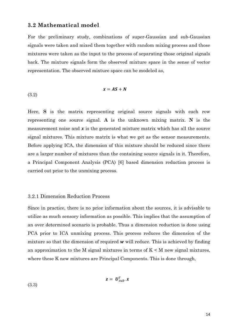
3.2 Mathematical model

For the preliminary study, combinations of super-Gaussian and sub-Gaussian

signals were taken and mixed them together with random mixing process and those

mixtures were taken as the input to the process of separating those original signals

back. The mixture signals form the observed mixture space in the sense of vector

representation. The observed mixture space can be modeled as,

(3.2)

Here, S is the matrix representing original source signals with each row

representing one source signal. A is the unknown mixing matrix. N is the

measurement noise and is the generated mixture matrix which has all the source

signal mixtures. This mixture matrix is what we get as the sensor measurements.

Before applying ICA, the dimension of this mixture should be reduced since there

are a larger number of mixtures than the containing source signals in it. Therefore,

a Principal Component Analysis (PCA) [6] based dimension reduction process is

carried out prior to the unmixing process.

3.2.1 Dimension Reduction Process

Since in practice, there is no prior information about the sources, it is advisable to

utilize as much sensory information as possible. This implies that the assumption of

an over determined scenario is probable. Thus a dimension reduction is done using

PCA prior to ICA unmixing process. This process reduces the dimension of the

mixture so that the dimension of required will reduce. This is achieved by finding

an approximation to the M signal mixtures in terms of K < M new signal mixtures,

where these K new mixtures are Principal Components. This is done through,

(3.3)

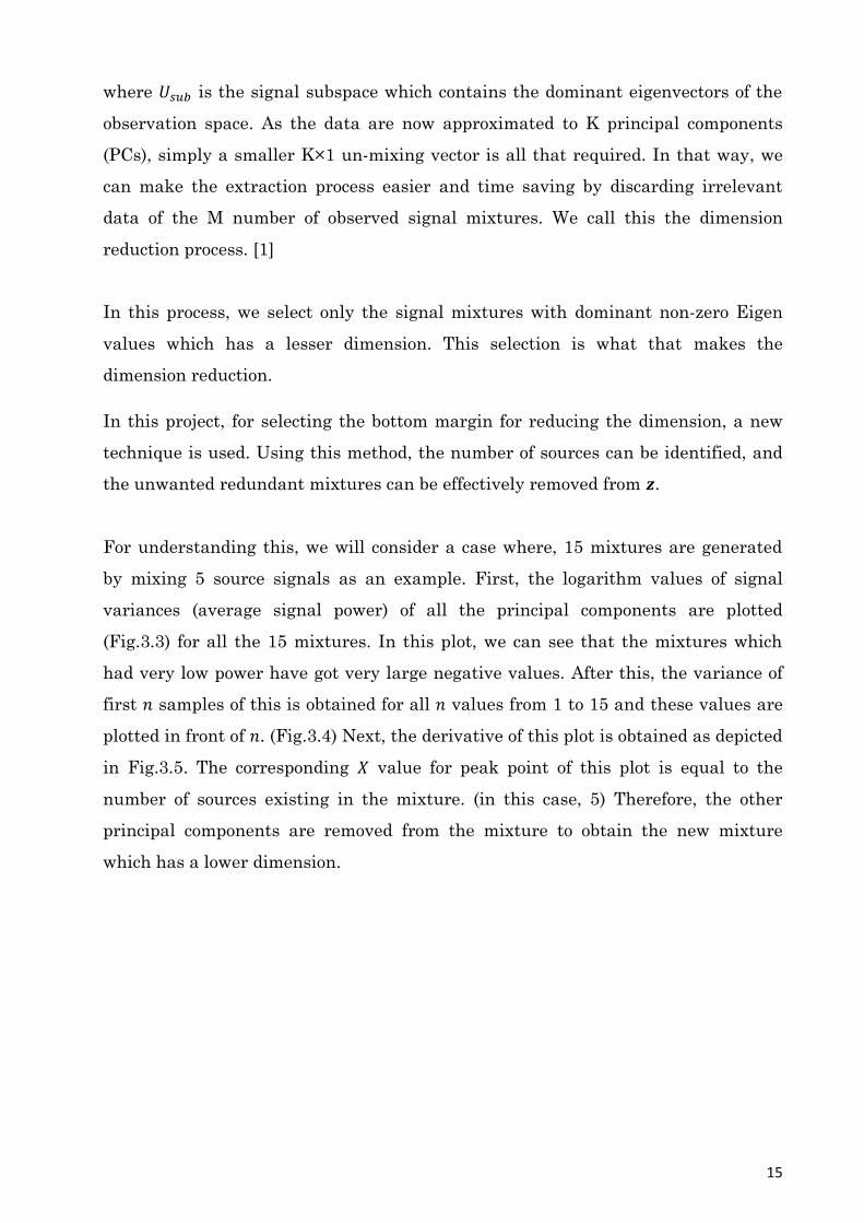
15

where is the signal subspace which contains the dominant eigenvectors of the

observation space. As the data are now approximated to K principal components

(PCs), simply a smaller K×1 un-mixing vector is all that required. In that way, we

can make the extraction process easier and time saving by discarding irrelevant

data of the M number of observed signal mixtures. We call this the dimension

reduction process. [1]

In this process, we select only the signal mixtures with dominant non-zero Eigen

values which has a lesser dimension. This selection is what that makes the

dimension reduction.

In this project, for selecting the bottom margin for reducing the dimension, a new

technique is used. Using this method, the number of sources can be identified, and

the unwanted redundant mixtures can be effectively removed from .

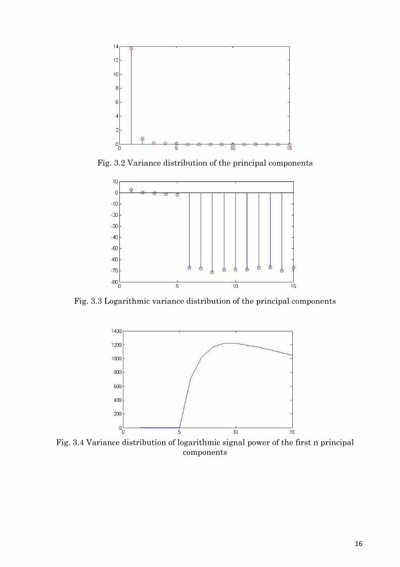
For understanding this, we will consider a case where, 15 mixtures are generated

by mixing 5 source signals as an example. First, the logarithm values of signal

variances (average signal power) of all the principal components are plotted

(Fig.3.3) for all the 15 mixtures. In this plot, we can see that the mixtures which

had very low power have got very large negative values. After this, the variance of

first samples of this is obtained for all values from 1 to 15 and these values are

plotted in front of . (Fig.3.4) Next, the derivative of this plot is obtained as depicted

in Fig.3.5. The corresponding value for peak point of this plot is equal to the

number of sources existing in the mixture. (in this case, 5) Therefore, the other

principal components are removed from the mixture to obtain the new mixture

which has a lower dimension.

16

Fig. 3.2 Variance distribution of the principal components

Fig. 3.3 Logarithmic variance distribution of the principal components

Fig. 3.4 Variance distribution of logarithmic signal power of the first n principal

components

17

Fig. 3.5 Derivative of variance distribution of logarithmic signal power of the first n

principal components

3.2.2 Unmixing Process

An unmixing weight vector is applied to the dimension reduced mixture of for

source extraction. It is tuned such that the kurtosis of the resultant output signal is

maximized for a super-Gaussian source (or minimized for sub-Gaussian source).

For a mixture with 2 source signals, after dimension reduction, the normalized

weight vector to be tuned takes the form,

(

), (3.4)

where is the independent variable in the brute force approach. This satisfies the

basis of having | | as well. (According to the identity,√ )

Using the Kurtosis as a measure of non-Gaussianity, we can now examine how the

kurtosis of a signal y = extracted from a set of K < M mixtures vary with the

weight vector . Note that here, is the dimension reduced space where you have

the un-correlated set of signal mixtures.

Z =

(3.5)

(3.6)

18

Weight vector is rotated around the origin with respect to For each value of ,

the associated kurtosis is plotted as a distance from the origin in the direction of ,

giving a continuous curve. We called this plot the polar plot for the kurtosis

variation.

3.2.3 Un-mixing sources from a mixture of four signals

Four acoustic source signals containing different music were used as the sources. As

shown in the Fig.3.3 they were mixed randomly and modeled exactly the same way

as it is discussed in equation 3.2. Our target was to extract the original sources back

without using any of the information related to those source signals.

Fig. 3.6 Original sources

19

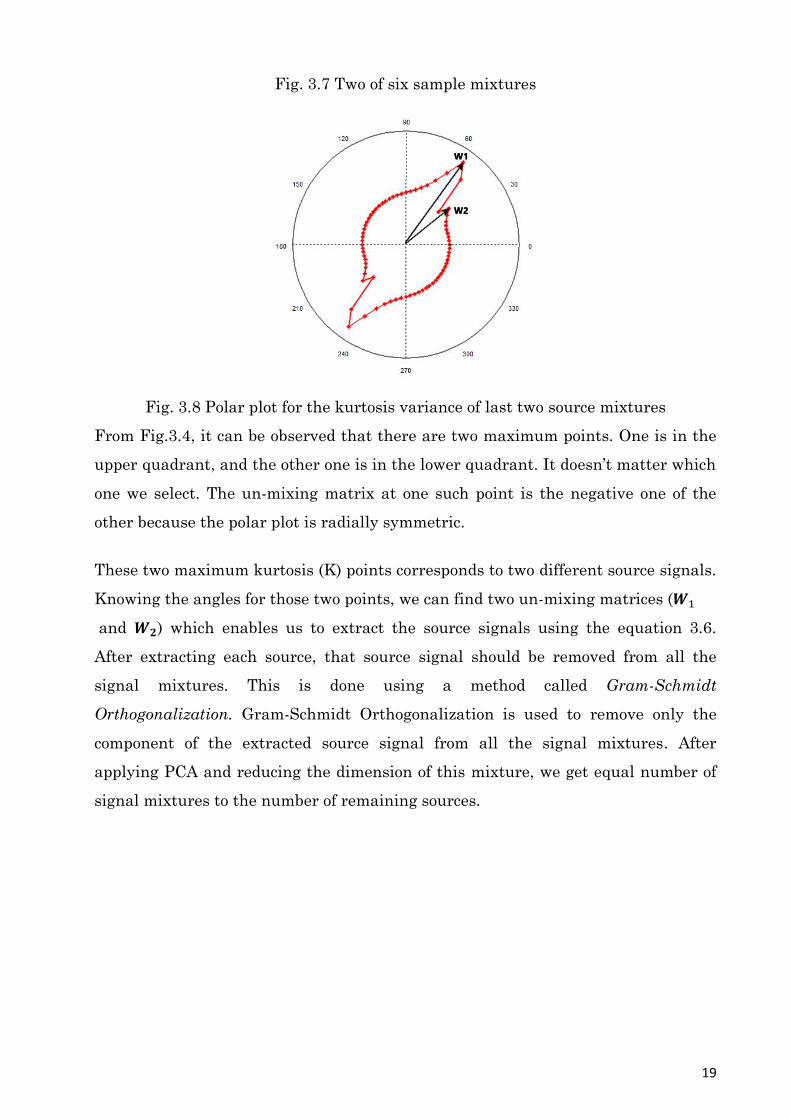
Fig. 3.7 Two of six sample mixtures

Fig. 3.8 Polar plot for the kurtosis variance of last two source mixtures

From Fig.3.4, it can be observed that there are two maximum points. One is in the

upper quadrant, and the other one is in the lower quadrant. It doesn’t matter which

one we select. The un-mixing matrix at one such point is the negative one of the

other because the polar plot is radially symmetric.

These two maximum kurtosis (K) points corresponds to two different source signals.

Knowing the angles for those two points, we can find two un-mixing matrices (

and ) which enables us to extract the source signals using the equation 3.6.

After extracting each source, that source signal should be removed from all the

signal mixtures. This is done using a method called Gram-Schmidt

Orthogonalization. Gram-Schmidt Orthogonalization is used to remove only the

component of the extracted source signal from all the signal mixtures. After

applying PCA and reducing the dimension of this mixture, we get equal number of

signal mixtures to the number of remaining sources.

20

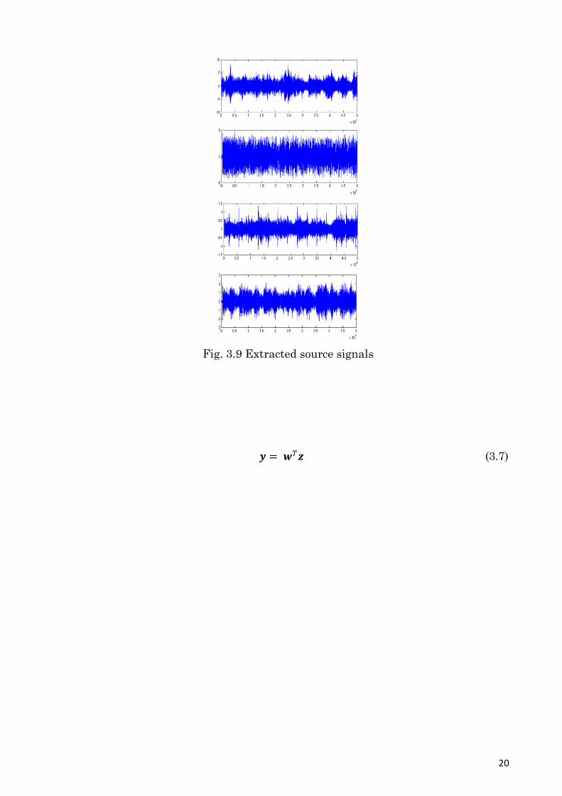
Fig. 3.9 Extracted source signals

(3.7)

21

Fig. 3.10 Comparison of the original sources and the extracted ones

It can be seen that the extracted signals are mostly the same as the original source

signals before mixing process.

3.3 Conclusions: Limitations for the Brute force method

Generally, the brute force approach would give us good results. But, finding the

maximum/ minimum points on the kurtosis surface is computationally exhaustive

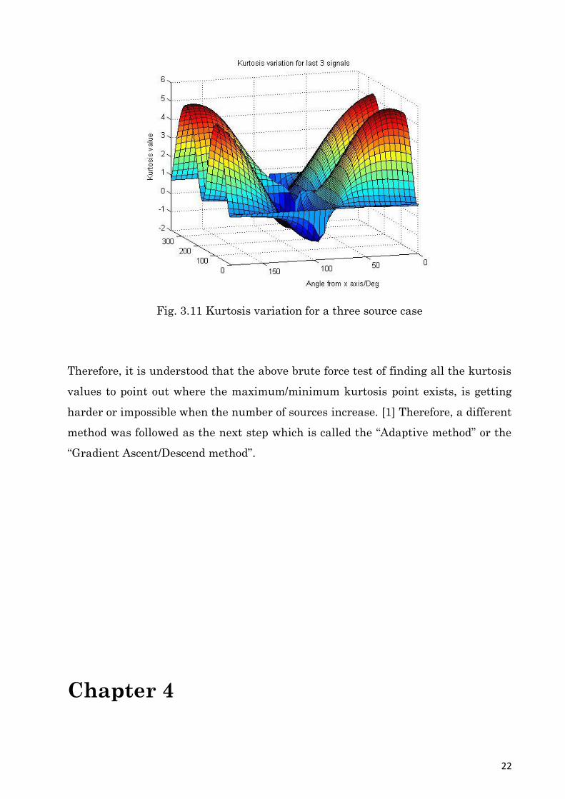
task to accomplish. For three signal mixtures, the kurtosis variation will be a 3-

dimensional surface as shown in Fig 3.6. For n number of signals, this will be an n-

dimensional surface. Therefore, in this approach, the computational complexity

increases exponentially with the number of source signals. On the other hand, this

method is less accurate since it is not practically possible to check for all the

possible weight vectors because there is infinite number of possibilities for the

weight vector in the n-dimensional space.

22

Fig. 3.11 Kurtosis variation for a three source case

Therefore, it is understood that the above brute force test of finding all the kurtosis

values to point out where the maximum/minimum kurtosis point exists, is getting

harder or impossible when the number of sources increase. [1] Therefore, a different

method was followed as the next step which is called the “Adaptive method” or the

“Gradient Ascent/Descend method”.

Chapter 4

23

Source Extraction by Gradient

based Algorithms

4.1 Introduction

We know that, in practice, the statistical independence can be used to separate

sources from a set of noisy mixtures. The more independent the extracted signals

are, the more likely they are to be the required source signals. Yet, we haven’t

considered a method for maximizing such measures like independence other than

by the brute force method which we discussed in Chapter 3. Brute force method

becomes an exhaustive exercise to deal with as the number of source signals

increase beyond four. Moreover, it wastes the time and the processing power which

can be vital in practical cases. Therefore, we have to have several alternative

methods which bring us better search strategies to accomplish the task.

Due to these reasons, the gradient ascend/descend method is introduced. This

method is based on the observation that if it is desired to reach the top of the hill or

the very bottom of the hill, the one simple strategy is to keep moving until there is

no more uphill (for gradient ascend) or no more downhill (for the gradient descend)

left. Therefore, our ultimate destination should be the peak point or the bottom

point.[1]

The kurtosis measures the non-Gaussianity. And also we know that the

independence means more non-Gaussianity. The height of the surface corresponds

to the amount of kurtosis. And the weight vector corresponds to different values of

the two un-mixing coefficients. We increase the kurtosis to pick the un-mixing

coefficients related to any super-Gaussian signal we want to extract. For a sub-

Gaussian source we should go down to a local minimum of the kurtosis surface to

pick the related coefficients.

Starting from the initial point on the kurtosis surface, we move in the direction of

the steepest slope or the gradient of the surface. Along the direction of gradient, one

24

step down assures the kurtosis of the extracted signal become less whereas one step

uphill assures an extracted signal with a higher kurtosis.

The most efficient method to find the direction of steepest slope at a given point is

to calculate the rate of change or the derivative of the local kurtosis with respect to

each un-mixing coefficient. At a given point, the gradient of kurtosis is different for

each un-mixing coefficient. Together, their combined gradients define the direction

on the ground plane. As a fact, this direction corresponds to a direction of

ascend/descend on the kurtosis surface. The gradient of the kurtosis surface with

respect to the weight vector is given by,

[ ] (4.1)

In order to make the step to the next point on the kurtosis surface, we add a

multiplier of this gradient to the previous We use proven recurrence formulae to

perform the gradient ascent with respect to the un-mixing parameters.

(4.2)

Here, is sufficiently small value to make sure the convergence at the top point of

the hill. In this method, is guaranteed to extract a signal with a higher

kurtosis than the signal extracted by .

In the same manner, for the gradient descent, the recurrence formulae will be in the

form,

(4.3)

Now we can make our step to a new point along the direction of the steepest

gradient using the recurrence formulae. Then again we have to find the direction to

proceed in the same way that we have done calculations for the previous point.

Likewise, beginning from an initial point, we can follow the direction along the

steepest gradient and finally stop at a local maximum or a local minimum point on

the kurtosis surface.

25

Note that the gradient descent will work only for the sub-Gaussian signals. For the

mixtures which have only the sub-Gaussian signals in it, we can straight away use

gradient descent.

At the same time, the gradient ascent will work only for the super-Gaussian

signals. For the mixtures which have only the super-Gaussian signals in it, we can

straight away use gradient ascent.

What if there are both super-Gaussian and sub-Gaussian sources are available in

the mixtures?

As we know, the gradient ascent method extract super-Gaussian source signals

whereas the gradient descent method extract sub-Gaussian sources from the given

signal mixtures. But real world signal mixtures comprise of both type of source

signals. Therefore, we cannot use only one method straight away for source

extraction from such mixtures. Accordingly, before we start this gradient based

adaptive method, we have to make sure which kind of a source signal is going to be

extracted in the first place.

It is a known thing that the sub-Gaussian signals have negative kurtosis value and

super-Gaussian signals have positive kurtosis value. Thus, the sign of the K gives

us the impression which kind of a signal we are dealing with. Here, our criterion is

the sign of the kurtosis at the initial point where we start the gradient based

algorithm. We have added a simple modification to our gradient based recurrence

formulae to make it easier.

(4.4)

Note that we calculate K at the initial point. Our logic is that if the initial K value is

positive, there should be at least one super-Gaussian signal, and if the initial K

value is negative, there should be at least one sub-Gaussian source signal within

the mixture.

26

To summarize, if the kurtosis at the initial point on the kurtosis surface is positive,

our algorithm switches to the normal gradient ascent algorithm. Otherwise, it

switches to the gradient descend algorithm.

Note that the critical points (maxima and minima) corresponding to the sources are

local ones. Each local maxima/minima corresponds to a source signal to be

extracted. In order to make sure we reach a maximum or the minimum point of the

kurtosis surface, we need an effective convergence criterion.

4.2 The convergence criteria

It is understood that we can use different criteria or else combinations of them to

seek the best one for testing the convergence. At the end of the day, what we need is

the un-mixing coefficients which can extract the source signals with a minimum

error. We stop the gradient ascend/descend process when we reach the convergence

point. There are the three basic criteria that we can count on.

4.2.1 Minimum gradient

This is with the simple argument that, if the gradient value is zero (or very close to

zero), that point should be a critical point (maxima or minima). Practically, we

cannot assure that we reach the critical point exactly. Therefore, the gradient value

may or may not be zero. Here we have some tolerance level.

Gradient can be calculated as follows. Note that Z is for the sphered mixtures and y

is what we extracted from this process.

Gradient wK =

(4.5)

4.2.2 Minimum kurtosis difference between two adjacent points

Whenever we get closer to a critical point on a surface, the kurtosis difference of two

adjacent points should be clearly decreasing. In that way we can fairly approximate

27

the critical point. For example, when the kurtosis difference is less than 0.00001 it

can be assumed that we have reached the critical point.

4.2.3 Checking the stability of the weight vector

Above two methods have their own drawbacks since if the kurtosis value of the

source signal is relatively small, it is difficult to get accurate extraction of the

source since this kurtosis difference or the gradient value can be always very small

for such case even if the weight vector has not reached closer to the peak point of

the kurtosis surface.

To counter this problem, weight vector stability checking method is proposed. When

we get closer to a critical point on the kurtosis surface, changing speed of the weight

vector becomes smaller. This means, when the weight vector becomes constant, we

can stop the gradient ascent/descent process. The stability of the weight vector can

be checked only for a certain number of decimal points. This is because, even after

reaching the local maxima or minima, there will be very small changes in the

weight vector because practically, we cannot assure that the weight vector reaches

the maximum point exactly.

This method is the preferable as this method uses the weight vector to identify the

convergence. Weight vector is what that determines the extracted source signal.

Therefore, if the weight vector is stationary, there is no point of continuing the

gradient ascent/descent process because the extracted sources will be the same.

4.3 Preliminary work

Before the gradient ascent process, the basic pre-processing of signal mixtures

should be done. First, the signal mixtures should be normalized. After that, we do

the dimension reduction process using PCA and again the normalizing is done.

After that, we do the sphering and then again normalize the resulting mixtures.

After that, the mixtures are ready for the gradient ascent or the descent process.

28

4.3.1 Gradient Ascent: Un-mixing a super Gaussian source signal

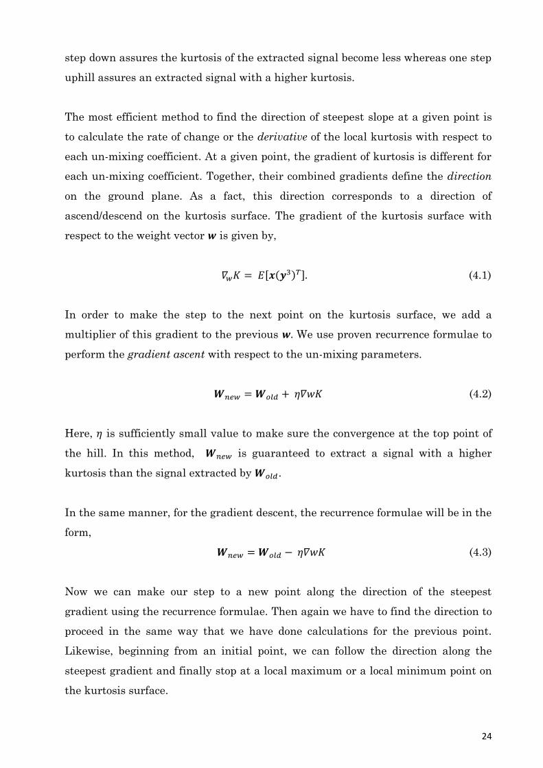
Starting from the initial weight vector , the gradient ascent was performed

and the results were taken. Note that here we are following a reduced space where

‖ ‖ = 1. We stopped after checking the stability of the weight vector for 100

iterations. We took that point as a local maximum point of the kurtosis surface.

Fig. 4.1 Reaching the maximum kurtosis by the gradient ascent

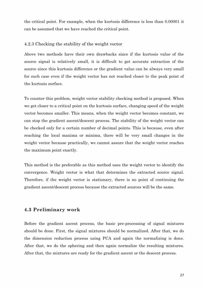
Fig. 4.2 Kurtosis variation for the gradient ascent.

29

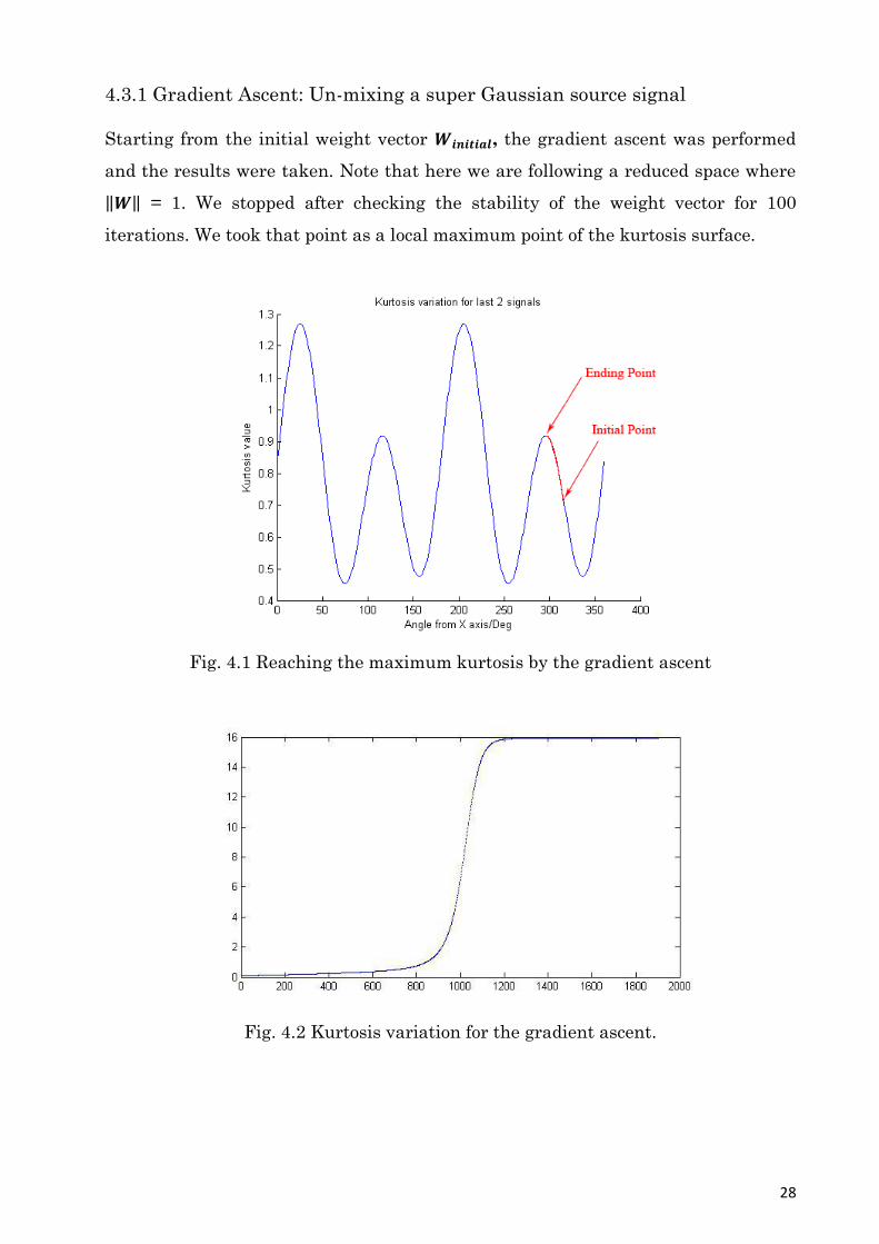
Fig. 4.3 Variation of first component of the weight vector for the gradient ascent.

When we extract source signals one at a time converging to the corresponding local

maximum points, there is a possibility to get the same source signal again and

again. Specially, when there are many source signals inside the mixtures, it is

probable this repetition occurs more often. Therefore, once we get a source, we have

to remove it from the mixtures and then continue with the gradient ascent. In this

scenario, we use Gram-Schmidt orthogonalization which we discussed in previous

chapter under brute force approach as well.

4.3.2 Gradient Descent: Un-mixing a sub Gaussian source signal

Same procedure was followed as for the gradient ascent but here we try to catch the

corresponding local minima points by moving in the negative gradient direction. For

this, equation 4.3 is utilized. We went downwards along the kurtosis surface to

achieve the un-mixing matrix at the kurtosis minima. Once we extracted a source,

set of new mixtures were sorted out by using Gram-Schmidt Orthogonalization.

Throughout the whole process, we used each and every step, normalization,

dimension reduction, sphering and finally the Gram-Schmidt Orthogonalization to

get the results.

30

Fig. 4.4 Reaching the minimum kurtosis point for a sub Gaussian source signal.

Fig. 4.5 Kurtosis variation for gradient descent

Fig. 4.6 Variation of first component of the weight vector for the gradient ascent.

31

4.4 Results and conclusions

4.4.1 Un-mixing the mixture with 4 source signals

Fig. 4.7 Two samples of six mixtures used

From the obtained results, we can see that the extracted sources and the original

ones are almost the same.

(a) (b)

Fig. 4.8 (a) Original sources (b) extracted sources

32

So that we can conclude that this gradient based adaptive method is successful and

it has many advantages like easier calculations, better approximation of the

sources, ability to apply for all super-super, super-sub and sub-sub cases for the

source signals. And we do not want to know any of the information related to the

source signals. But in this kurtosis based approach, we have to extract sources one

by one. And we cannot predict the order in which the source signals are extracted.

33

Chapter 5

Extension of ICA for Complex

Valued Mixtures

For real signals mixed through a real gain matrix, the above real valued ICA

method reliably works for super Gaussian, sub Gaussian or super-sub coupled

mixtures and for any number of sources as long as they are independent and non-

Gaussian. But in some scenarios, the real sources can be mixed through a certain

complex valued gain so that the mixtures are complex valued. Under such cases, it

is necessary to extend the ICA algorithm for a complex kurtosis based algorithm [4].

This complex valued ICA method is just a generalization of real valued algorithm so

that this algorithm can be used for both cases when the mixing matrix is real

valued as well as when the mixing matrix is complex valued. To extend the ICA

algorithm for a complex valued algorithm, we need to determine complex kurtosis

and its gradient.

5.1 Complex kurtosis and its gradient

Kurtosis of a complex valued signal is still a real number. The kurtosis of a complex

valued signal can be written as,

[ ] [ ] [ ] . (5.1)

5.2 Gradient of Kurtosis

Although the signals are complex, the objective of ICA is same. In particular, even

for complex valued signals, the Gaussianity implies zero kurtosis, super-

Gaussianity implies positive kurtosis and sub-Gaussianity implies negative

kurtosis. Therefore, un-mixing an independent signal from a set of complex valued

measurement signals given by , would involve finding a complex valued weight

34

vector such that the unmixed complex valued signal would yield a source. This

involves optimizing the kurtosis of over as before. In principle, it should be

possible to use a gradient based algorithm for this optimization process similar to

that in the real valued case.

Under the classical definition of the complex differentiation, is not differentiable

in as it is a real valued function of complex variable. However, it is possible to

utilize Wirtinger calculus [4] to find the gradient of over . Wirtinger calculus is a

popular choice in many complex valued signal processing applications including

adaptive signal processing [10].

5.2.1 Definition: Wirtinger Differential Operator

Let is a complex number with x and y being the real and imaginary parts

respectively. Then, the Wirtinger Differential operator is denoted by

and written

as,

, (5.2)

where and are arbitrary constants. Typically they are set to

and

.

With this definition, using above a1 and a2, and when is the conjugate

of , we can immediately write down,

. (5.3)

If is a scalar function of a complex vector , we can extend the

Wirtinger derivative operator to obtain the gradient of kurtosis in terms of

analogous to the real counterpart:

. (5.4)

As defined in (5.1), the kurtosis of the extracted signal consists of three parts:

[ ] [ ] and [ ] where . Therefore, we need the gradient of

35

each of these components with respect to the complex variable . In particular, it is

needed to find [ ] [ ] and [ ] .

Using the definitions (5.2), (5.3), and (5.4) it can be shown that,

[ ] ( [ ]

[ ]

)

,

[ ] [ ]. (5.5)

[ ] ( [ ]

[ ]

)

,

[ ] [ ] [ ] (5.6)

Furthermore, since

[ ]

[ ] [ ]

,

[ ]

[ ] [ ] . (5.7)

We get,

[ ] [ ] [ ] [ ]

[ ] [ ] [ ]. (5.7)

Combining these results the gradient of the complex kurtosis described in (5.1) can

be expressed as,

[ ] [ ] [ ]

[ ] [ ] [ ] [ ] [ ]. (5.8)

36

5.3 Update equation

There would not be any difference in the update equation which is used for real

valued ICA except the conjugate gradient of kurtosis. So the update equation for

complex mixtures can be expressed as,

* (5.9)

5.4 Unmixing source signals using complex valued ICA

Starting from the initial complex valued weight vector , the gradient ascent

was performed for a complex valued signal mixture generated by a complex valued

mixing matrix and the results were taken. The gradient ascent process was stopped

after checking the stability of weight vector for 100 iterations.

5.4.1 Un-mixing the mixture with 4 source signals

The real parts of the two signal mixtures and the extracted source signals are

shown in Fig.5.1 and Fig.5.2 respectively. From the obtained results, we can see

that the extracted sources and the original ones are almost the same.

Fig. 5.1 Two of six mixtures used

37

(a) (b)

Fig. 5.2 (a) Original sources (b) extracted sources using complex valued ICA

So that we can conclude that the gradient based adaptation method for complex

valued ICA is successful for extraction of source signals mixed through a complex

valued mixing matrix.

38

Chapter 6

Frequency domain ICA for source

extraction in frequency domain

As we have discussed previously, the complex valued ICA method can be effectively

used for extraction of independent source signals from signal mixtures which are

mixed using a complex valued mixing matrix. But for non-linear mixing processes,

it is not possible to use complex valued algorithm to extract sources. This is

because, when the mixture is convolutive (non-linear), the source extraction cannot

be done in time domain. Therefore, complex valued ICA algorithm cannot be

directly used to extract non-linearly mixed source signals. Therefore, a frequency

domain unmixing process should be used to extract sources under these conditions

[5]. To extend the complex valued ICA algorithm to a frequency domain unmixing

algorithm, the mixture matrix is converted to frequency domain by applying the

Fast Fourier transform [11] to each row of the matrix separately. Then, the same

complex valued ICA process is carried out for extracting sources while remaining in

the frequency domain. After extracting the source signals, the output matrix is

again converted back to time domain by applying the inverse Fast Fourier

transform operation. The real or imaginary part of the resulting vectors will

represent the sources.

6.1 Unmixing source signals using frequency domain ICA

Starting from the initial complex valued weight vector , the gradient ascent

was performed in frequency domain for a complex valued signal mixture generated

using a complex valued mixing matrix. The gradient ascent process was stopped

after checking the stability of weight vector for 100 iterations, and the results were

obtained.

39

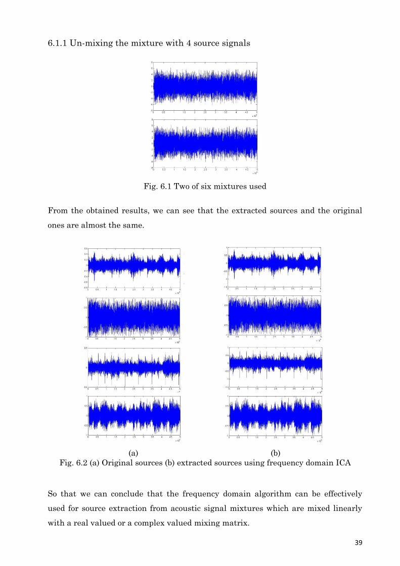
6.1.1 Un-mixing the mixture with 4 source signals

Fig. 6.1 Two of six mixtures used

From the obtained results, we can see that the extracted sources and the original

ones are almost the same.

(a) (b)

Fig. 6.2 (a) Original sources (b) extracted sources using frequency domain ICA

So that we can conclude that the frequency domain algorithm can be effectively

used for source extraction from acoustic signal mixtures which are mixed linearly

with a real valued or a complex valued mixing matrix.

40

Chapter 7

Application of ICA for acoustic

signal mixtures

7.1 Possible applications

Generally, ICA has been applied to countless applications in vast array of fields

related to signal processing, neuroimaging, face recognition [9], mobile phone

communications and even for analyzing and predicting the stock market prices.

The algorithms and the theory developed in this project can be directly use for some

applications. We targeted our algorithms for two types of cases. They are, for

acoustic signals and images. As discussed in the previous chapters, all three

algorithms were capable of effectively extracting sources from a mixture of linearly

mixed acoustic source signals. In this chapter, first, the performance of the three

algorithms for linear acoustic signal mixtures is compared.

7.2 Extracting sources from linear acoustic signal mixtures

7.2.1 Results

As we discussed previously, two time domain algorithms and frequency domain

algorithm could extract sources successfully from acoustic signal mixtures which

were mixed linearly. All the results produced by the three algorithms for linear

acoustic signal mixtures and used original source signals are shown in Fig.7.1.

41

(a) (b) (c) (d)

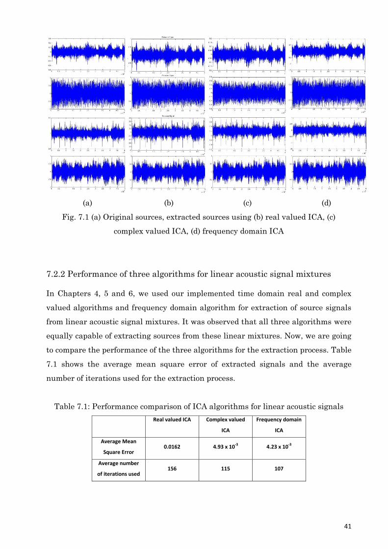
Fig. 7.1 (a) Original sources, extracted sources using (b) real valued ICA, (c)

complex valued ICA, (d) frequency domain ICA

7.2.2 Performance of three algorithms for linear acoustic signal mixtures

In Chapters 4, 5 and 6, we used our implemented time domain real and complex

valued algorithms and frequency domain algorithm for extraction of source signals

from linear acoustic signal mixtures. It was observed that all three algorithms were

equally capable of extracting sources from these linear mixtures. Now, we are going

to compare the performance of the three algorithms for the extraction process. Table

7.1 shows the average mean square error of extracted signals and the average

number of iterations used for the extraction process.

Table 7.1: Performance comparison of ICA algorithms for linear acoustic signals

Real valued ICA Complex valued

ICA

Frequency domain

ICA

Average Mean

Square Error 0.0162 4.93 x 10

-3 4.23 x 10

-3

Average number

of iterations used 156 115 107

42

These results clearly indicate that the complex valued time domain algorithm and

frequency domain algorithm have better accuracy for extracted sources from linear

acoustic signal mixtures. Out of the two complex valued algorithms, frequency

domain algorithm showed slightly better results. When it comes to speed, frequency

domain algorithm was the fastest while real valued algorithm being the slowest.

Both complex valued algorithms are equally capable of extracting sources when the

source signal mixtures are real valued or complex valued. But the real valued

algorithm is only capable of extracting sources when they are mixed with a real

valued mixing matrix.

7.3 Extracting sources from non-linear acoustic signal

mixtures

Due to linear time domain unmixing process, the time domain ICA algorithms are

highly limited to applications where the mixing process is assumed to be linear.

When the mixing process is non-linear, these algorithms fail to produce desirable

results. Therefore, it is important to go for the frequency domain algorithm which

can capture these non-linearities so that convoluted temporal signals generated by

non-linear mixing processes can be extracted.

Blind source separation of convoluted acoustic signals is of great interest for many

categories of applications such as audio editing, speech recognition, hands-free

telephony or hearing devices. Due to the convolutive mixing process, the unmixing

process should be done in frequency domain. This is done via the frequency domain

complex valued ICA algorithm. In this project, only one kind of a non-linearity is

discussed and reliable extraction of sources is demonstrated.

7.3.1 Process of extraction

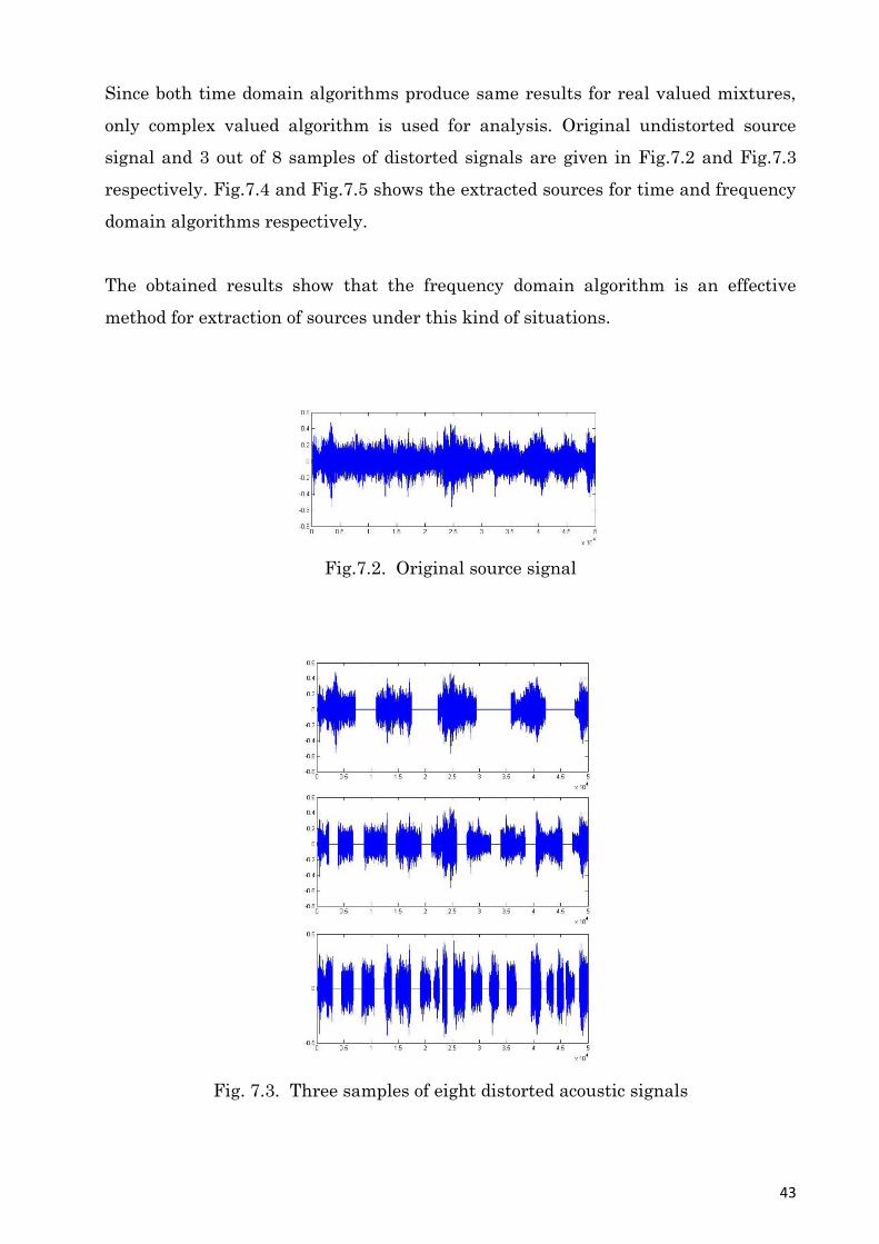
We will take 8 acoustic signals in which all the signals are distorted by making

randomly selected regions zero such that there is no single sound signal which

represents the complete source signal. These 8 signals were used as the rows of the

mixture matrix and the time and frequency domain algorithms were applied.

43

Since both time domain algorithms produce same results for real valued mixtures,

only complex valued algorithm is used for analysis. Original undistorted source

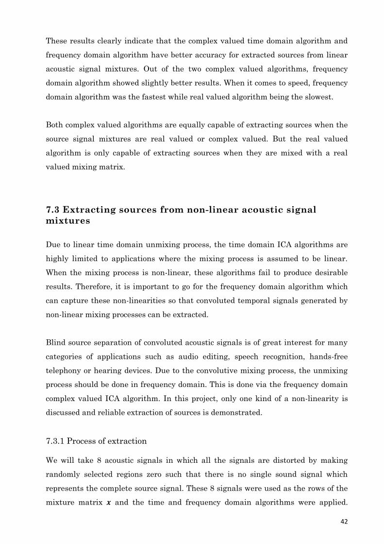
signal and 3 out of 8 samples of distorted signals are given in Fig.7.2 and Fig.7.3

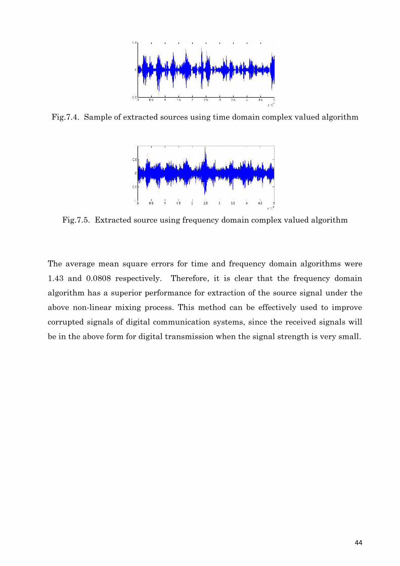
respectively. Fig.7.4 and Fig.7.5 shows the extracted sources for time and frequency

domain algorithms respectively.

The obtained results show that the frequency domain algorithm is an effective

method for extraction of sources under this kind of situations.

Fig.7.2. Original source signal

Fig. 7.3. Three samples of eight distorted acoustic signals

44

Fig.7.4. Sample of extracted sources using time domain complex valued algorithm

Fig.7.5. Extracted source using frequency domain complex valued algorithm

The average mean square errors for time and frequency domain algorithms were

1.43 and 0.0808 respectively. Therefore, it is clear that the frequency domain

algorithm has a superior performance for extraction of the source signal under the

above non-linear mixing process. This method can be effectively used to improve

corrupted signals of digital communication systems, since the received signals will

be in the above form for digital transmission when the signal strength is very small.

45

Chapter 8

Application of ICA for extracting

sources from image mixtures

Image restoration based blind source separation techniques are widely used in

many applications such as, vision based surveillance applications, face recognition

[9], MRI etc. The above ICA algorithms can be directly use for extraction of sources

from a set of images.

As we discussed above, conventional time domain ICA algorithms assume the signal

mixtures to be linear. Therefore, time domain algorithms cannot be effectively used

when the mixtures are non-linear convoluted mixtures. These, non-linearities

include phase delays, occlusion, distortion of the waveform/ image etc. The

frequency domain implementation of the algorithm enables reliable separation of

occluded content under various foreground disturbance conditions. In this chapter,

the performance of the frequency domain algorithm is analyzed and compared for

image restoration with the time domain ICA algorithms.

8.1 Application of ICA techniques for image mixtures

For application of the ICA algorithm to images, first the images should be converted

to one-dimensional signals. Therefore, before applying ICA, the images are

converted into 1-dimensional signals by breaking up the rows of the image and

stacking or concatenating them together as shown by the Fig 8.1. After this, the

resulting vectors can be arranged as rows of the matrix where each row

representing one unwrapped image and each column represents a particular pixel’s

value for all the images.

46

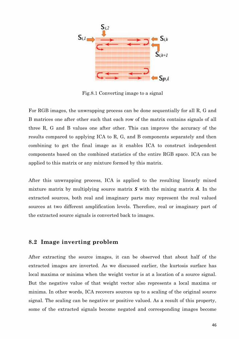
Fig.8.1 Converting image to a signal

For RGB images, the unwrapping process can be done sequentially for all R, G and

B matrices one after other such that each row of the matrix contains signals of all

three R, G and B values one after other. This can improve the accuracy of the

results compared to applying ICA to R, G, and B components separately and then

combining to get the final image as it enables ICA to construct independent

components based on the combined statistics of the entire RGB space. ICA can be

applied to this matrix or any mixture formed by this matrix.

After this unwrapping process, ICA is applied to the resulting linearly mixed

mixture matrix by multiplying source matrix with the mixing matrix . In the

extracted sources, both real and imaginary parts may represent the real valued

sources at two different amplification levels. Therefore, real or imaginary part of

the extracted source signals is converted back to images.

8.2 Image inverting problem

After extracting the source images, it can be observed that about half of the

extracted images are inverted. As we discussed earlier, the kurtosis surface has

local maxima or minima when the weight vector is at a location of a source signal.

But the negative value of that weight vector also represents a local maxima or

minima. In other words, ICA recovers sources up to a scaling of the original source

signal. The scaling can be negative or positive valued. As a result of this property,

some of the extracted signals become negated and corresponding images become

47

inverted. Therefore, a method for detecting and re-correcting the inverted images is

required. In order to detect the inverted images, a new method was proposed in this

work. For understanding this method, let’s take a look at the waveforms of inverted

and un-inverted 8-bit images shown in Fig 8.2 (a) and (b) respectively.

(a) (b)

Fig.8.2 Unwrapped signal of a (a) un-inverted image (b) inverted image

From the waveforms, it can be observed that in the waveform of un-inverted image,

most of the pixel values are below 255/2, and for the inverted image, most of the

pixel values are above 255/2. Therefore, the number of pixels is counted for two

cases where the pixel value is larger than 255/2 and smaller than 255/2 for all three

R, G and B matrices of the image. If the number of pixels which have higher value

than 255/2 is greater than the number of pixels which have lower value than 255/2,

then the image is considered to be inverted.

This method can be generalized based on context where for each application the

general unwrapped images statics such as RGB mean etc. are analyzed to detect

inverted images.

After finding the inverted images using this method, those images are inverted back

in the algorithm to get proper un-inverted images. Any image under normal

lighting conditions can be detected using this method.

48

8.3 Applying ICA to linear image mixtures

In order to test the algorithms for a linear mixture of images, the matrix

containing four images are mixed through a real valued mixing matrix . Note that

here, a real valued mixing matrix is used for testing purposes since the real valued

time domain algorithm is only capable of handling real valued mixtures. The

complex valued algorithm is equally capable of handling real valued mixtures as

well as complex valued mixtures.

The obtained results show that, both real and complex valued ICA algorithms

produce the same results, except that the complex valued ICA algorithm was much

faster and accurate compared to the real valued algorithm. It was also observed

that the frequency domain ICA algorithm failed to produce desirable results when

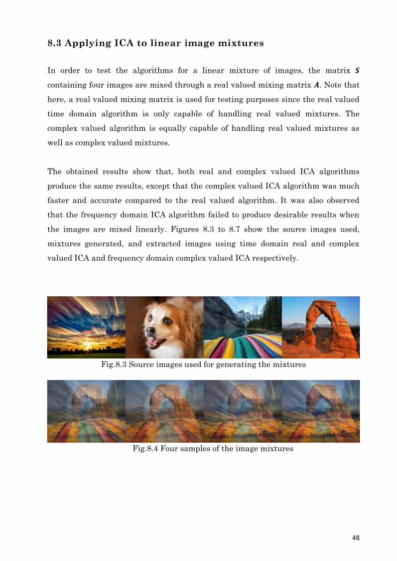
the images are mixed linearly. Figures 8.3 to 8.7 show the source images used,

mixtures generated, and extracted images using time domain real and complex

valued ICA and frequency domain complex valued ICA respectively.

Fig.8.3 Source images used for generating the mixtures

Fig.8.4 Four samples of the image mixtures

49

Fig.8.5 Extracted sources for real valued ICA with ŋ = 0.1 and stabilizing w for

5 decimal points

Fig.8.6 Extracted sources for complex valued time domain ICA with ŋ = 1 and

stabilizing w for 4 decimal points

Fig.8.7 Extracted sources for complex valued frequencydomain ICA with ŋ = 1

and stabilizing w for 4 decimal points

As can be observed from the obtained results in Fig.8.5, 8.6 and 8.7, it is clear that

the complex valued time domain ICA algorithm has superior performance compared

with the real valued time domain algorithm even when lower number of decimal

points is used for stabilizing the weight vector for the complex valued ICA

algorithm. Therefore, complex valued ICA algorithm has better performance in

terms of both speed and the accuracy. The real and complex valued algorithms took

231 and 122 average number of iterations respectively for extraction of the four

images. Another fact is that in the real valued ICA algorithm, as ŋ is increased, the

accuracy of the obtained results goes down. But for the complex valued time domain

ICA algorithm, as ŋ is increased, both the accuracy and the speed of the extraction

process increase. But if ŋ is increased too much, sometimes there is a problem for

50

convergence so that it takes longer time to extract the sources. This property helps

to successfully manipulate the parameter to get the best performance from the

complex valued algorithm.

The obtained results for frequency domain algorithm (Fig. 8.7.) clearly shows that

the frequency domain algorithm does not produce desirable results for linearly

mixed image mixtures as linear mixing in time domain implies convoluted mixing

in frequency domain.

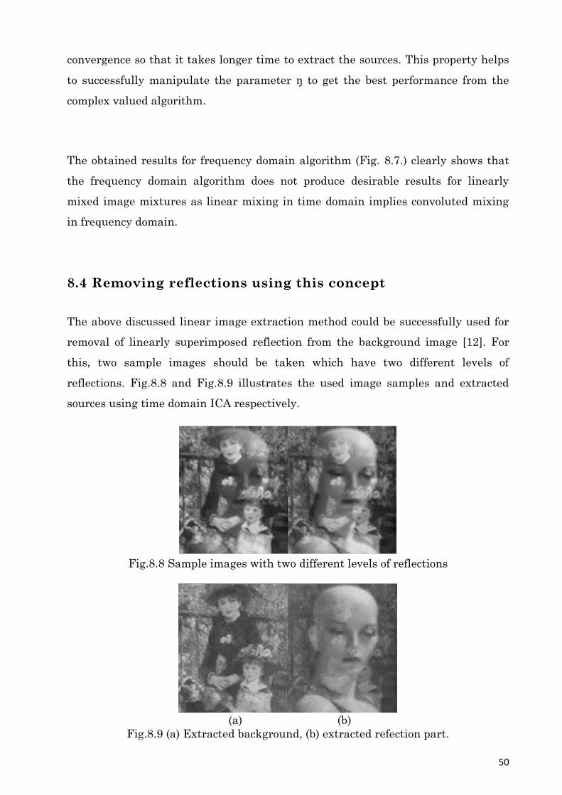
8.4 Removing reflections using this concept

The above discussed linear image extraction method could be successfully used for

removal of linearly superimposed reflection from the background image [12]. For

this, two sample images should be taken which have two different levels of

reflections. Fig.8.8 and Fig.8.9 illustrates the used image samples and extracted

sources using time domain ICA respectively.

Fig.8.8 Sample images with two different levels of reflections

(a) (b)

Fig.8.9 (a) Extracted background, (b) extracted refection part.

51

Two different levels of reflections as in this example can be practically obtained by

placing a polarizing filter in front of the camera lens before taking the photograph.

For most modern cameras, a circular polarizer is typically used. Since reflections

tend to be at least partially linearly-polarized, a linear polarizer can be used to

change the balance of the light in the photograph so that the reflection level in the

photograph can be changed accordingly. The rotational orientation of the filter can

be adjusted for the preferred effect in the photograph and two different levels of

reflections can be obtained from the photograph exactly as explained in this

example.

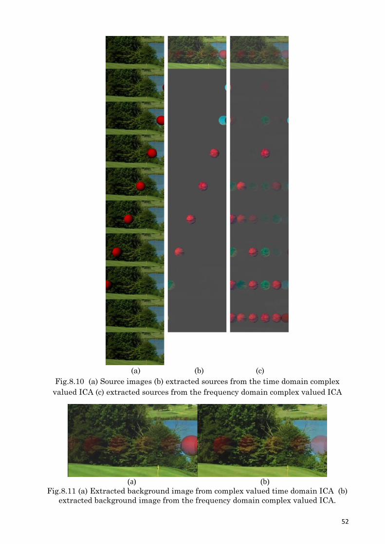
8.5 Extracting sources from non-linear image mixtures

As examples for non-linear image mixtures, two examples were taken where the

background of the image is occluded by foreground disturbances. These kinds of

occlusions are a result of non-linear mixing process of images. This means this kind

of images cannot be represented as a linear superposition of two or more images.

But in above discussed examples, all the mixtures were linear super-positions of the

source images required to be extracted.

In order to represent an occluded example, first, a sample image set was taken

where a ball passes across the background. The image set consists of ten image

frames where in each image the ball moves a little bit through the background

scene. In the set of ten images, there are two images which have completely visible

background without any occlusion caused by the ball in the foreground. Source

images and the obtained results for both time domain and frequency domain

complex valued ICA algorithms are given in Fig. 8.10 (a), (b), and (c) respectively.

Fig. 8.11 compares the obtained background image.

52

(a) (b) (c)

Fig.8.10 (a) Source images (b) extracted sources from the time domain complex

valued ICA (c) extracted sources from the frequency domain complex valued ICA

(a) (b)

Fig.8.11 (a) Extracted background image from complex valued time domain ICA (b)

extracted background image from the frequency domain complex valued ICA.

53

This case is taken as non-linear since the ball and the background image is not a

linear superposition of two or more images unlike in earlier cases. As can be

observed from the obtained results, it is possible to state that the complex valued

time domain ICA algorithm could separate the foreground ball and the background

scene of the image clearly. But the frequency domain algorithm could not extract

the foreground ball properly. This shows that, for this kind of situations, complex

valued time domain method is better for foreground extraction as a complex mixing

in the time domain is more representative for this scenario. But as depicted in

Fig.8.11. (a) and (b) it can be seen that the frequency domain algorithm yields

better results for the separated image of the background.

As mentioned above, in the above example, the input source image set contains two

images in which the background is completely visible without any foreground

occlusion. This makes it easier for the algorithms to separate the background and

foreground of the image set.

8.6 Extracting background using frequency domain ICA

As mentioned above, in the above example, the input source image set contains two

images in which the background is completely visible without any foreground

occlusion. This makes it easier for the algorithms to separate the background and

foreground of the image set.

Therefore, next we will consider an example in which the source image set does not

contain any image that the background is completely visible. This means all the

images are occluded by some foreground disturbance. For this, a black line grid is

used to cover the background of an image. And for each image, the foreground grid

is shifted horizontally by a small amount randomly. Target was to extract the

background of the image using ICA. The used source image samples, extracted

sources using time and frequency domain ICA algorithms are given in Fig 8.12, 8.13

and 8.14 respectively. Note that the position of the foreground grid used in the

source images are not the same. This is a typical case in surveillance applications.

54

Fig.8.12 Three samples of the 10 occluded source images

Fig.8.13 Extracted image using time domain complex valued ICA algorithm

Fig.8.14 Extracted image using frequency domain complex valued ICA algorithm

The obtained results clearly show that only the frequency domain algorithm is

capable of extracting the background image as the time domain complex valued

algorithm does not produce a proper extraction of the background.

8.7 Conclusion

For most image mixtures, real valued ICA algorithm and the time domain complex

valued algorithm reliably estimates the sources if the underlying mixing process is

linear and real valued. However, the complex valued ICA algorithm showed faster

convergence and more accurate results compared to the time domain real valued

55

algorithm. When the mixing process is complex valued, the real valued time domain

algorithm cannot be used for source extraction. It is also possible to say that when

the mixing process is linear, the frequency domain algorithm cannot be used for

extracting the sources properly as a result of convoluted frequency domain mixing.

However, the linear image extraction method was successfully used to remove a

foreground reflection using time domain ICA when the reflection is linearly

superimposed on the background image. When the mixing process is non-linear,

such as in the occluded case discussed above, it was observed that the time domain

algorithms were incapable of providing desirable results. Therefore, the frequency

domain implementation of ICA should be used for source extraction under non-

linear occlusive mixtures.

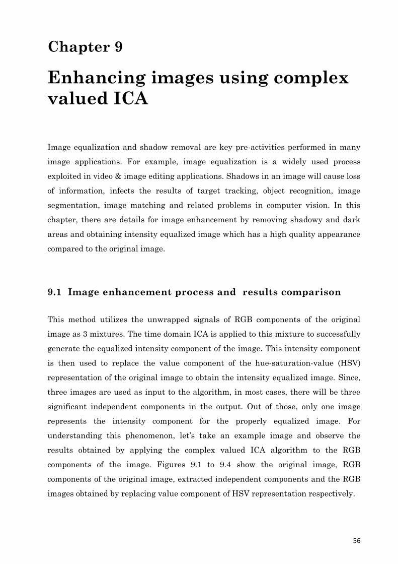
56

Chapter 9

Enhancing images using complex

valued ICA

Image equalization and shadow removal are key pre-activities performed in many

image applications. For example, image equalization is a widely used process

exploited in video & image editing applications. Shadows in an image will cause loss

of information, infects the results of target tracking, object recognition, image

segmentation, image matching and related problems in computer vision. In this

chapter, there are details for image enhancement by removing shadowy and dark

areas and obtaining intensity equalized image which has a high quality appearance

compared to the original image.

9.1 Image enhancement process and results comparison

This method utilizes the unwrapped signals of RGB components of the original

image as 3 mixtures. The time domain ICA is applied to this mixture to successfully

generate the equalized intensity component of the image. This intensity component

is then used to replace the value component of the hue-saturation-value (HSV)

representation of the original image to obtain the intensity equalized image. Since,

three images are used as input to the algorithm, in most cases, there will be three

significant independent components in the output. Out of those, only one image

represents the intensity component for the properly equalized image. For

understanding this phenomenon, let’s take an example image and observe the

results obtained by applying the complex valued ICA algorithm to the RGB

components of the image. Figures 9.1 to 9.4 show the original image, RGB

components of the original image, extracted independent components and the RGB

images obtained by replacing value component of HSV representation respectively.

57

Fig.9.1: Original image used for equalization

(a) (b) (c)

Fig.9.2: (a) Red component of the image. (b) Green component of the image. (c)

Blue component of the image.

(a) (b) (c)

Fig.9.3: Extracted images from RGB components using complex ICA algorithm

(a) (b) (c)

Fig.9.4: RGB images obtained by replacing value component of HSV image with

the extracted independent components (a), (b), (c) separately

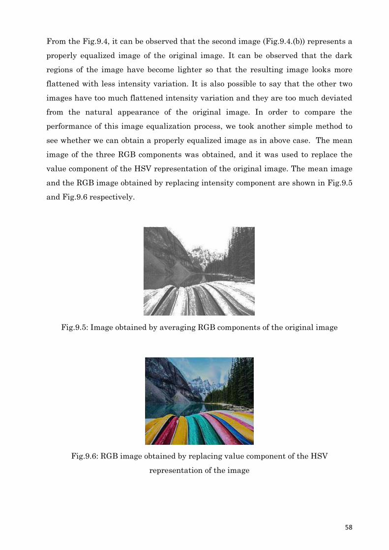
58

From the Fig.9.4, it can be observed that the second image (Fig.9.4.(b)) represents a

properly equalized image of the original image. It can be observed that the dark

regions of the image have become lighter so that the resulting image looks more

flattened with less intensity variation. It is also possible to say that the other two

images have too much flattened intensity variation and they are too much deviated

from the natural appearance of the original image. In order to compare the

performance of this image equalization process, we took another simple method to

see whether we can obtain a properly equalized image as in above case. The mean

image of the three RGB components was obtained, and it was used to replace the

value component of the HSV representation of the original image. The mean image

and the RGB image obtained by replacing intensity component are shown in Fig.9.5

and Fig.9.6 respectively.

Fig.9.5: Image obtained by averaging RGB components of the original image

Fig.9.6: RGB image obtained by replacing value component of the HSV

representation of the image

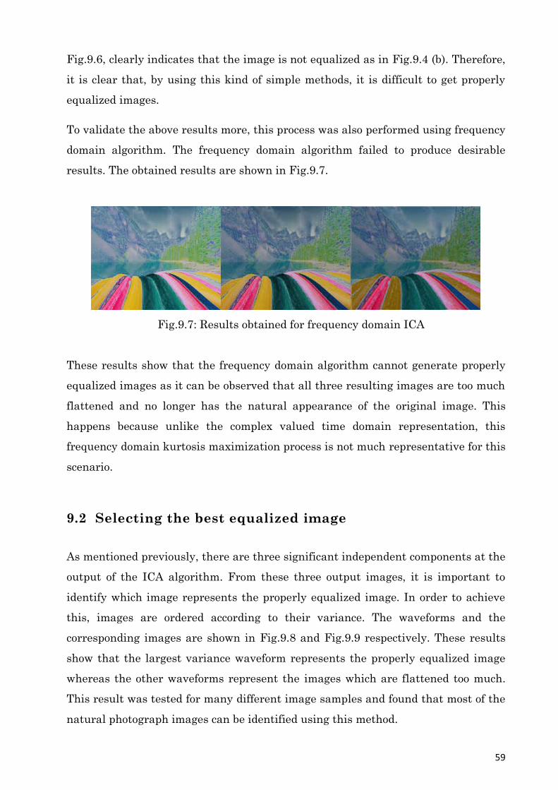
59

Fig.9.6, clearly indicates that the image is not equalized as in Fig.9.4 (b). Therefore,

it is clear that, by using this kind of simple methods, it is difficult to get properly

equalized images.

To validate the above results more, this process was also performed using frequency

domain algorithm. The frequency domain algorithm failed to produce desirable

results. The obtained results are shown in Fig.9.7.

Fig.9.7: Results obtained for frequency domain ICA

These results show that the frequency domain algorithm cannot generate properly

equalized images as it can be observed that all three resulting images are too much

flattened and no longer has the natural appearance of the original image. This

happens because unlike the complex valued time domain representation, this

frequency domain kurtosis maximization process is not much representative for this

scenario.

9.2 Selecting the best equalized image

As mentioned previously, there are three significant independent components at the

output of the ICA algorithm. From these three output images, it is important to

identify which image represents the properly equalized image. In order to achieve

this, images are ordered according to their variance. The waveforms and the

corresponding images are shown in Fig.9.8 and Fig.9.9 respectively. These results

show that the largest variance waveform represents the properly equalized image

whereas the other waveforms represent the images which are flattened too much.

This result was tested for many different image samples and found that most of the

natural photograph images can be identified using this method.

60

(a) (b) (c)

Fig.9.8: Waveforms of the images when they are ordered according to variance

in descending order with (a) largest, (b) second largest and (c) smallest variance

waveform.

(a) (b) (c)

Fig.9.9: Images corresponding to (a), (b) and (c) of Fig.9.8.

9.3 Conclusions

Complex valued time domain ICA is capable of generating intensity equalized

images when photographed or natural images are used. But the frequency domain

algorithm could not produce properly equalized images. Furthermore, the proposed

variance based method can be successfully used to identify the correct independent

components.

61

Chapter 10

Conclusions

In this project, time domain real and complex valued ICA algorithms and a complex

valued frequency domain algorithm were implemented for source extraction from

linear and non-linear acoustic signal mixtures and image mixtures. For acoustic

signals, both time and frequency domain algorithms were effective for extracting

sources if the mixing process is linear. But only frequency domain algorithm was

successful for source extraction from the discussed non-linear corrupted acoustic

signal mixture. This was because of the convoluted time domain mixing behavior of

the non-linear mixtures. However, the complex valued ICA algorithm showed faster

convergence and more accurate results compared to the time domain real valued

algorithm. The algorithms were also used for source extraction from linear and non-

linear image mixtures which can be used for some synthetic and typical image

restoration problems. For most image mixtures, real valued ICA algorithm and the

time domain complex valued algorithm reliably estimates the sources if the

underlying mixing process is linear and real valued. When the mixing process is

complex valued, the real valued time domain algorithm cannot be used for source

extraction. It is also possible to say that when the mixing process is linear, the

frequency domain algorithm cannot be used for extracting the sources from images

properly, as a result of convoluted frequency domain mixing. However, the linear

image extraction method was successfully used to remove a foreground reflection

using time domain ICA when the reflection is linearly superimposed on the

background image. When the mixing process is non-linear, such as in the occluded

case discussed in this project, it was observed that the time domain algorithms were

incapable of providing desirable results. Therefore, the frequency domain

implementation of ICA is used for source extraction under non-linear occlusive

mixtures and the reliable extraction of sources under such cases was demonstrated

for image restoration. Finally, a new image equalizing method was proposed and it

was found that the ICA time domain implementations are capable of generating

intensity equalized images when photographed or natural images are used.

Furthermore, the proposed variance based method can be successfully used to

62

identify the correct independent component from three intensity components

extracted using time domain ICA.

Finally, we can conclude that the proposed ICA based BSS methods in this project

perform really well in many different applications and they are highly competitive

and feasible ways of separating independent source signals out of a mixture.

63

References

[1] James V Stone, Independent component analysis; a tutorial, 2nd ed., Bradford

book, The MIT press, England, 2002.

[2] Hyva¨rinen,nE. Oja, “Independent Component Analysis: Algorithms and

Applications”，Neural Networks, vol.13,pp. 411- 430,2000.

[3] J. C. Rajapakse and W. Chen, “Complex ICA-R,” in Neural Networks (IJCNN),

The 2010 International Joint Conference on, 2010, pp. 1–8.

[4] W. V. D. Wijesinghe, G. Godaliyadda, M. P. B. Ekanayake, and H. K. Garg,

“Department of Electrical and Electronic Engineering, University of Peradeniya,

Sri Lanka,” in Industrial and Information Systems (ICIIS), 2013 8th IEEE

International Conference on, 2013, pp. 144–149.

[5] P. Smaragdis, "Blind Separation of convolved mixtures in the frequency

domain," Neurocomputing, Vol. 22, pp.21-34, 1998.

[6] I.T. Jolliffe. Principal Component Analysis. Springer-Verlag,1986

[7] Anemüller, Jörn, Terrence J. Sejnowski, and Scott Makeig. “Complex

Independent Component Analysis of Frequency-Domain

Electroencephalographic Data.” Neural Networks 16, no. 9 (November 2003):

1311–23. doi:10.1016/j.neunet.2003.08.003.

[8] Biswal, Bharat B.; Ulmer, John L., “Blind Source Separation of Multiple Signal

Sources of fMRI Data Sets Using Independent Component Analysis”, Journal of

Computer Assisted Tomography: March/April 1999.

[9] Kinage, Kishor S., and S. G. Bhirud. “Face Recognition Using Independent

Component Analysis of GaborJet (GaborJet-ICA).” In Signal Processing and Its

64

Applications (CSPA), 2010 6th International Colloquium on, 1–6. IEEE, 2010.

http://ieeexplore.ieee.org/xpls/abs_all.jsp?arnumber=5545318.

[10] Farhang -Boroujeny, B., Adaptive Filters Theory and Applications, John Wiley

and Sons, Chichester, UK, 1998.

[11] Mateer, Todd. “Fast Fourier Transform Algorithms with Applications.”

Clemson University, 2008. http://cr.yp.to/f2mult/mateer-thesis.pdf.

[12] M. Bronstein, M. M. Bronstein, M. Zibulevsky, and Y. Y. Zeevi, “Blind

separation of reflections using sparse ica,” in Proc. Int. Conf. ICA2003, Nara,

Japan, 2003, pp. 227–232.