General rights Copyright and moral rights for the publications made accessible in the public portal are retained by the authors and/or other copyright owners and it is a condition of accessing publications that users recognise and abide by the legal requirements associated with these rights.

• Users may download and print one copy of any publication from the public portal for the purpose of private study or research. • You may not further distribute the material or use it for any profit-making activity or commercial gain • You may freely distribute the URL identifying the publication in the public portal

If you believe that this document breaches copyright please contact us providing details, and we will remove access to the work immediately and investigate your claim.

Downloaded from orbit.dtu.dk on: Sep 06, 2018

Field calibration of cup anemometers

Kristensen, Leif; Jensen, G.; Hansen, A.; Kirkegaard, P.

Publication date:2001

Document VersionPublisher's PDF, also known as Version of record

Link back to DTU Orbit

Citation (APA):Kristensen, L., Jensen, G., Hansen, A., & Kirkegaard, P. (2001). Field calibration of cup anemometers.(Denmark. Forskningscenter Risoe. Risoe-R; No. 1218(EN)).

Risø–R–1218(EN)

Field Calibration of Cup Anemome-ters

Leif Kristensen,Gunnar Jensen,Ar ent Hansen,and Peter Kirk egaard

RisøNational Laboratory , Roskilde,Denmark

January 2001

Abstract�

An outdoorcalibrationfacility for cupanemometers,wherethesignalsfrom10 anemometersof which at leastone is a referencecan be can be recordedsimulta-neously, hasbeenestablished.The resultsare discussedwith specialemphasison thestatisticalsignificanceof thecalibrationexpressions.It is concludedthat themethodhasthe advantagethat many anemometerscanbe calibratedaccuratelywith a minimum ofwork andcost.Theobviousdisadvantageis that thecalibrationof a setof anemometersmaytakemorethanonemonthin orderto havewind speedscoveringasufficiently largemagnituderangein awind directionsectorwherewecanbesurethattheinstrumentsareexposedto identical,simultaneouswind flows. Anothermainconclusionis that statisti-cal uncertaintymustbe carefully evaluatedsincethe individual 10 minutewind-speedaveragesarenot statisticallyindependent.

ISBN 87–550–2772–5; ISBN 87–550–2773–3(Internet)ISSN0106–2840

Print:DankaServicesInternationalA/S, 2001

Contents

1 Intr oduction 5

2 Calibration Setup 6

3 Statistical Considerations 6

3.1 GainandOffsetby OrthogonalFitting 8

3.2 StatisticalUncertainties 11

4 Data Analysis 20

5 Conclusion 24

Appendices 28

A Regressionwith Curvature 28

B Monte Carlo Simulations 29

C DiscreteSampling 32

D Intermittent Sampling 34

Acknowledgements 40

References 41

Risø–R–1218(EN) 3

1 Intr oduction

Themostaccurateinstrumentfor measuringthemean-windspeedhasso-farbeenthecupanemometer. It wasinventedin 1846by theIrish astronomerT.R. Robinson(Middleton1969,Wyngaard1981)andthe original instrumentshadfour cups.Until the endof the1920smuch researchwent into experimentingwith the numberof cupsand the armlengths.Brazier(1914)andPatterson(1926)found that shorterarmsimprovedthe lin-earity of the calibrationand that a three-armcup rotor is optimal with respectto sen-sitivity andsuppressionof the unevennessin the rotation(“wobbling”). A moderncupanemometeris shown in Fig. 1.

Figure 1. TheRisøanemometer. Thediameterof theconicalcupsin the three-cupplastrotor is 7 cm. The body is madeof anodizedaluminum.The height of the instrumentfrom thebottomto thecenterof the rotor is 24.7cm.Theoutputsignal,generatedby amagneticallyactivatedswitch, is a train of electricpulses,two for each rotor revolution.By countingpulsesover a certain period one obtainsa numbercorrespondingto themean-windspeedfor this period.

Thecupanemometernow appearsto bethepreferredinstrumentfor measuringthemean-wind speedin thewind-energy community, mainly becauseof thelinearity, theaccuracyandthestabilityof thecalibration.But alsothefactthatthisinstrumentis omnidirectionalandeasyto mountmakes it attractive for routinemeasurements.Therehasbeensomediscussionaboutthe importanceof theso-called“overspeeding”which is causedby theasymmetricresponseto instantaneousincreasesand decreasesin the wind speedandwhich,incidentally, is anecessarypropertyfor thecupanemometerto startrotatingwhenexposedto a wind, i.e. to functionat all (Kristensen1998).Someof thosewho believethatoverspeedingis a problemhave preferredto usea propeller-vaneinstrumentwhichis consideredsymmetricin its responseto oppositewind directions.Theproblemis herethat thepropellersignaldependson the instantaneousanglebetweenthewind directionandthepropelleraxis.Thevaneof the instrument,which tries to align theaxiswith thewind direction,will alwayslagbehind.Theresultis thattherewill alwaysbeasystematicerrorof themeasuredmeanwind. Thiserroris in generalexacerbatedby thefactthatthepropellerwill performits own motionsinceit is seldommounteddirectlyovertheverticalaxis of the vane(Kristensen1994).Also, on basisof the studiesby Kristensen(1998),Kristensen(1999),andKristensen(2000)theadverseeffectsof theasymmetricresponseof the cupanemometerseemexaggerated.Thusthe choiceto usecupanemometersforroutinemeasurementsis asoundone.

In thefollowing we discussanoutdoorcalibrationsetupfor a numberof cupanemome-terswhich aresimultaneouslyexposedto the samewind. In principlewe canlet oneof

Risø–R–1218(EN) 5

the� anemometersbe“the standard”andthenintercalibrateby comparingtheoutputsig-nals.This standardanemometeris assumedto have beencalibratedin a “certified” wayaccordingto anapproved,well-describedmethodby meansof a goodwind tunnelwithlittle turbulenceandaflat profile.It couldbearguedthatananemometermountedoutdooris exposedto wind flowswhichchangesinstantaneouslyin bothwind speedandwind di-rectionwhereastheflow in awind tunnelis alwaysin thesamedirection.However, sincethe cup anemometerallegedly measuresthe instantaneouscomponent� we really com-paremeansignalsfrom theseoutdooranemometersthroughwhich the same“length ofair” haspassed,just aswe would have donewhenusinga wind tunnel.Theonly reser-vationonecanhave is that the non-idealangularresponseto verticalwind componentsmayproducea biasdueto thefluctuatingverticalwind component,but, asdemonstratedby Kristensen(1994),this canrelatively easilybequantifiedif necessary. Hereit is notconsidereda seriousproblem.

First we describethe calibrationsite.Thenwe discussthe statisticaldataanalysisand,finally, we illustratethemethodby analyzingrealdatafrom thecalibrationinstallation.

2 Calibration Setup

The calibrationsetupis locatedbehindthe beachat the southwesternpart of the Risøpeninsula,just north of the pier, asFig. 2 shows. The distanceto the water line is ap-proximately12m andtheorientationof thecalibrationboomwherethetenanemometersaremountedabout10 m over thesurroundingterrainis 19� –199� . This meansthatwindfrom the direction289� will have travelled over a water fetch of about7 km beforeitsimultaneouslyreachesall theanemometer. Acceptingadirectionsectorof � 45� around289� , thewaterfetchwill beat least3 km. In otherwords,thesitehasbeenchosento bewell-exposedfor windsfrom thepredominantwind directionin Denmark.

The calibrationboomis mountedon the top of two steel lattice mastswith triangularcrosssectionswith thesidelength0.25m. Fig. 3 showsasketchandaphotographof themeasuringsetup.

Thedatarecordingis carriedout with anAanderaadataloggerwith 12 ten-bit channels.Numberingthesefrom 1 to 12, channel1 is thetemperaturechannelandchannel12 thedirectionchannel.Channelsfrom 2 to 11areusedfor theanemometeroutputs.To preventthe signal from the Risøanemometerwith two countsper revolution from causingthe10-bit channelsto overflow during the countingperiod of 10 minutes,the numbersinthe registersarescaleddown by the factor25 � 32. Usually we have two positionsforreferenceanemometers.The rest of the positionsare test positions.Table 1 gives the“names”of thetenpositions.

Thiscalibrationconfiguration,whereuninterrupted,consecutive10-minuteaverageshavebeenmeasured,hasbeenoperatingsince1996.

3 Statistical Considerations

Thecalibrationprocedureimpliesthatwe comparetwo almostidenticalresponsesto thesamesignal.For symmetryreasonswe adopta methodwherethe meansquareof the�

Actually, averagedover onefull rotor rotation.

6 Risø–R–1218(EN)

Figure2.Mapof theRisøpeninsula.Thecalibrationsiteis shownin a little moredetail inthecircular blow-up.Thedirectionperpendicularto thecalibrationboom,which parallelto thecoastline, is 289 � . Whenthewindis fromthisdirectionthemutualflowdisturbancebetweentheanemometers is at minimum.

Figure 3. Calibration setupat Risø,in the left framedrawnto thescale1:190.Theori-entationof the boomwith the ten cup anemometers is 19 � –199� . Thelower boomis aserviceboomusedfor mountingthe instruments.Thewind directionis measuredat theendof a 1.8 m long boom,pointing in the direction319 � . Thethermometeris mountedona boomat 2 mover theground.Thetwo supportingmastsare triangular latticemastswith thesidelength25 cm.

Risø–R–1218(EN) 7

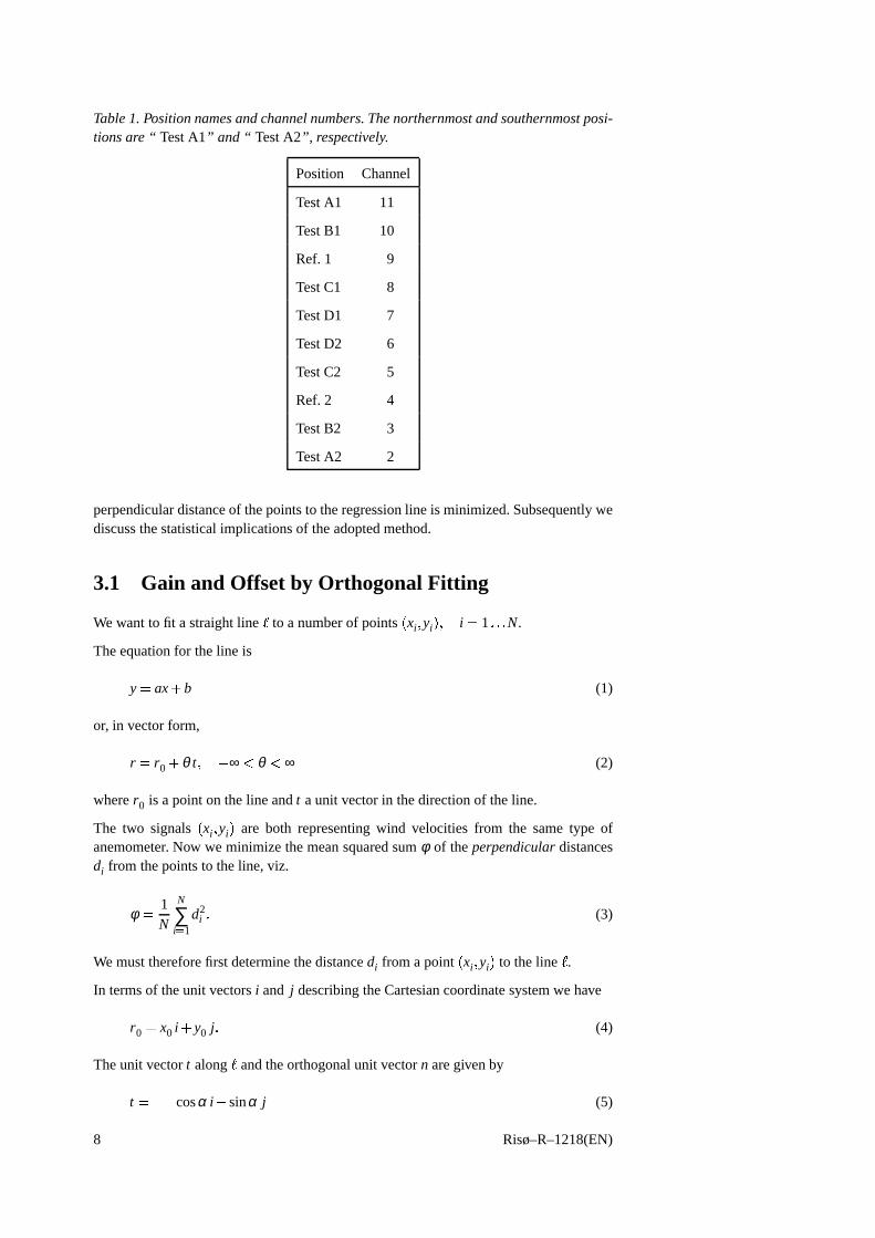
Table1. Positionnamesandchannelnumbers.Thenorthernmostandsouthernmostposi-tionsare “ TestA1” and“ TestA2”, respectively.

Position Channel

TestA1 11

TestB1 10

Ref.1 9

TestC1 8

TestD1 7

TestD2 6

TestC2 5

Ref.2 4

TestB2 3

TestA2 2

perpendiculardistanceof thepointsto theregressionline is minimized.Subsequentlywediscussthestatisticalimplicationsof theadoptedmethod.

3.1 Gain and Offset by Orthogonal Fitting

We wantto fit a straightline � to a numberof points � xi yi � i � 1 � � � N.

Theequationfor theline is

y � ax � b (1)

or, in vectorform,

r � r0 � θ t �� ∞ � θ � ∞ (2)

wherer0 is a point on theline andt aunit vectorin thedirectionof theline.

The two signals � xi yi are both representingwind velocities from the sametype ofanemometer. Now we minimizethemeansquaredsumφ of theperpendiculardistancesdi from thepointsto theline, viz.

φ � 1N

N

∑i � 1

d2i � (3)

We mustthereforefirst determinethedistancedi from a point � xi yi to theline � .In termsof theunit vectorsi and j describingtheCartesiancoordinatesystemwe have

r0� x0 i � y0 j � (4)

Theunit vectort along � andtheorthogonalunit vectorn aregivenby

t � cosα i � sinα j (5)

8 Risø–R–1218(EN)

and�n � � sinα i � cosα j (6)

whereα is theanglefrom thex-axisto � .Thesigneddistancedi from agivenpoint

r i� xi i � yi j (7)

to theline � is

di��� r i � r0 ��� n � � � xi � x0 sinα ��� yi � y0 cosα � (8)

Thedefinitionsof thequantitiesweuseareillustratedin Fig. 4.

�

�

�� �� �!

#"$ "%

&�')(+*-,/.103254

6

7

67 89 :;

Figure 4. Illustration of the calculationof the distancedi of onepoint to the regressionline with offsetb andslopea � tanα.

Equation(3) now becomes

φ � 1N

N

∑i � 1 < � � xi � x0 sinα ��� yi � y0 cosα = 2 � (9)

We want to determinethe valuesof r0 and α that minimize φ . In fact, thereare onlytwo independentparametersof which theangleα mustbeone.Sincewe expectα to bedifferentfrom n > π ? 2,wecanfix eitherof x0 ory0 andusetheotherasafitting parameter.Let usfix x0. In principle,thereis noboundson its value,but it seemspracticalto choosex0� x wheretheaveragesymbolstandsfor theoperation

z � 1N

N

∑i � 1

zi � (10)

Risø–R–1218(EN) 9

To@ find y0 wedemand

0 � ∂φ∂y0

� 1N

N

∑i � 1

2 A � � xi � x0 sinα ��� yi � y0 cosα BC� � cosα � 2cosα AD�E� x � x0 sinα � � y � y0 cosα B� � 2 � y � y0 cos2α (11)

which impliesthaty0� y.

For practicalreasonsweintroducenew coordinatesby moving theorigin to � x y andjustmake thefollowing replacements:FG H xi

yi

I JK : � FG H xi � x

yi � y

I JK (12)

sothat

φ � 1N

N

∑i � 1 < � xi sinα � yi cosα = 2 � (13)

To determineα we demandthat∂φ ? ∂α � 0:

0 � 2N

N

∑i � 1 < � xi sinα � yi cosα = < � xi cosα � yi sinα =� 2

N

N

∑i � 1 < � xi

2 � yi2 � cosα sinα � xiyi

� cos2α � sin2α � =� 2 LNM x2 � y2 O cosα sinα � xy � cos2α � sin2α �QP � (14)

Thesolutionto (14) is

tan2α � 2xy

x2 � y2(15)

or

tanα � 12xy

Ry2 � x2 �TS M y2 � x2 O 2 � 4xy

2 U � (16)

We seethat thereare two solutionsand that their productis � 1. This correspondstoslopeswhich minimize ( � solution)andmaximize( � solution)φ andwhich pertaintolineswhichareperpendicularto oneanother. We mustusethe � solution.

Introducing

δ � 12

ln V x2

y2 W (17)

10 Risø–R–1218(EN)

and�ε � 1

2ln XY x2 y2

xy2 Z[ � � ln �]\ ρ \ � (18)

where

ρ � xyM x2 y2 O 1̂ 2(19)

is thesamplecorrelationcoefficient,thenthesolution(16)canbewritten

a _ tanα � sign� xya`�b 1 ��� eε sinhδ 2 � eε sinhδ cd� (20)

and

b � y0 � ax0� y � ax � (21)

In appendixA wegeneralizetheapproachto allow for a slight curvature.

3.2 Statistical Uncertainties

In the following we will make repeateduseof the so-callederror-propagationformulaand,to setthe stageanddefinethe notation,we will reiterateits meaningandcontent.Then we will determinethe statisticaluncertaintiesof a and b and functionsof thesetwo quantities.Finally, we will determineif all theN realizationscanbeconsideredsta-tistically independentin the presentcontext or whetherwe mustreducethe degreesoffreedom.

Err or Propagation

Let

z � � z1 z2 �]� � zM (22)

be one realizationof a set of M ordered,randomvariableswhich may or may not beinter-correlated.†

Theensembleaveragesandvariancesof theM variablesof zare �]e z1 f e z2 f �]� � e zM f and�]g � z1 � e z1 f 2 h g � z2 � e z2 f 2 h � � � g � zM � e zM f 2 h � , respectively.

We may now considera smoothfunction f � z andconsiderits ensembleaverageandvariance.Expandingf � z to secondorder, we obtaine f � z fji f � e zf � 1

2

M

∑i � 1

M

∑j � 1

f k ki j �]e zf ml � zi � e zi f M zj � e zj f Oon (23)

†It is importantto notethat thesubscriptsheredenoteM differentstochasticprocessesandnot asin othercontexts thenumberof oneof theN realizationsor trials.

Risø–R–1218(EN) 11

and� l � f � zp� e f � z f 2 n i M

∑i � 1

f ki � e zf M

∑j � 1

f kj � e zf ql � zi � e zi f M zj � e zj f Oon (24)

whereprimesindicatepartialdifferentiationwith respectto thevariablewith thenumbersin thelower indices.

Thelastequationshowsthemechanismof errorpropagation:thestatisticaluncertaintyofasinglerandomvariablez is oftenrepresentedby avariance,theso-callederrorvariance(see,e.g.Lenschow et al. (1994)).Theerrorvarianceof a function f � z of z will thenbedeterminedbyl � f � zp� e f � z f 2 n i f k 2 � e zf e � z � e zf 2 f � (25)

Whentherearemorethanonerandomvariablethe uncertaintyof eachvariablezi mayagainbedeterminedby its errorvariancewhereastheuncertaintyof a functionof thesevariableswill includeall the possiblecovariancesof pairsof zi andzj . For example,inthecaseof two randomvariableswehave

l � f � z1 z2 p� e f � z1 z2 f � 2 ni f k12 � e z1 f e z2 f e]� z1 � e z1 f 2 f � f k22 � e z1 f e z2 f e]� z2 � e z2 f 2 f� 2 f k1 � e z1 f e z2 f f k2 �]e z1 f e z2 f e]� z1 � e z1 f e � z2 � e z2 f f � (26)

A straightforwardgeneralizationof (24) to covariancesbetweentwo functions f � z andg � z will alsobeneededin thefollowing.

er� f � zq� e f � z f � g � zp� e g � z f fi M

∑i � 1

f ki � e zf M

∑j � 1

gk j � e zf l � zi � e zi f M zj � e zj f Oon � (27)

BasicStatisticsfor Pairs

We assumethat the pairs � xi yi , i � 1 2 � �]� N are independentand identically dis-tributed.Without lossof generalitywe may alsoassumethat they have zeroensemblemeans.

Theensemblevariancesarethene x2 f _se x2i f (28)

and e y2 f _se y2i f � (29)

We thereforehavethefollowing relationse xix j f � e x2 f δi j (30)

12 Risø–R–1218(EN)

e yiy j f � e y2 f δi j (31)

and e xiy j f �st e x2 f e y2 f ρ0 δi j (32)

whereρ0 is thecorrelationcoefficient.

Theensemblemeanscanof courseonly beestimatedby thesamplemeans.We have

x � 1N

N

∑i � 1

xi (33)

and

y � 1N

N

∑i � 1

yi (34)

andweassumethatN is solargethatwemayconsiderx i y i 0 goodapproximationstotheensemblemeans.

Thestatisticaluncertaintiesmeasuredin termsof thevariancesof thesamplesmeansarel � x � e xf 2 n � e x2 fN

(35)

and l � y � e yf 2 n � e y2 fN� (36)

Theensemblevariancesentering(35)and(36)areestimatedby thesamplevariances

x2 � 1N

N

∑i � 1

x2i (37)

and

y2 � 1N

N

∑i � 1

y2i � (38)

Similarly, thecovarianceof xi andyi andthecorrelationcoefficientareapproximatedby

xy � 1N

N

∑i � 1

xiyi (39)

and

ρ0� e xyfe x2 f 1̂ 2 e y2 f 1̂ 2 i xy

x21̂ 2y21̂ 2

� ρ � (40)

In order to determinethe variancesof x2, y2, and their covariancewe assumethat theprobabilitydensityof � xi yi is joint Gaussian.

Risø–R–1218(EN) 13

Wu

e� thenobtainv M x2 � g x2 h O 2 w � 2e x2 f 2

N (41)v M y2 � g y2 h O 2 w � 2e y2 f 2

N (42)

and l M x2 � g x2 h O M y2 � g y2 h Oon � 2e x2 f e y2 f

Nρ2

0 � (43)

Statistical Uncertaintiesof a and b

Now we have the tools for determiningthe statisticaluncertaintiesof a andb givenby(20)and(21).

In thepresentapplicationthetwo variablesx andy arehighly correlatedwith acorrelationcoefficientcloseto unity. They arealsoverycloseto beingidenticalwhichmeansthattheabsolutevalueof δ is muchsmallerthanone.This impliesthat(20) in erroranalysescansafelybeapproximatedby

a i 1 � δ � (44)

Using(26)with

f � z1 z2 � 1 � 12

ln ` z1

z2c (45)

with therandomvariablesFG H z1

z2

I JK � FG H x2

y2

I JK (46)

wehave

f k1 � z1 z2 � � 12z1

(47)

and

f k2 � z1 z2 � 12z2

(48)

sothatthevarianceof a becomes

σ2 A a Bx_ l � f � z1 z2 p� e f � z1 z2 f � 2 n� 14 y 2

N � 22ρ2

0

N� 2

N z � 1 � ρ20

N i 21 � ρ0

N� (49)

14 Risø–R–1218(EN)

This{ equationhasbeenconfirmedby a Monte Carlo simulationasdiscussedin the ap-pendixB.

Thevalueof a is in our casevery closeto one.We canthereforesimplify theexpressionfor b whencalculatingtheerrorvarianceof b asfollows

b � y � ax i y � x � (50)

In this case

f � z1 z2 � z2 � z1 (51)

with FG H z1

z2

I JK � FG H x

y

I JK (52)

sothat

σ2 A b B � e x2 f ��e y2 f � 2 e xyfN i x2 � y2 � 2xy

N� (53)

Finally, to beableto evaluatethestatisticaluncertaintyof functionsof a andb we needto determinethecovariance

µ A a b B �gQ� f � z1 z2 z3 z4 p� e f � z1 z2 z3 z4 f � � g � z1 z2 z3 z4 p� e g � z1 z2 z3 z4 f � h (54)

where F|||||||G |||||||H z1

z2

z3

z4

I |||||||J|||||||K �F|||||||G |||||||H x2

y2

x

y

I |||||||J|||||||K (55)

andwhere

f � z1 z2 z3 z4 � a � 1 � 12

ln ` z1

z2c (56)

and

g � z1 z2 z3 z4 � b � z4 � f � z1 z2 z3 z4 z3� z4 � z3 � z3

2ln ` z1

z2c}� (57)

Again,applying(27)we find thata andb areuncorrelated,thatis

µ A a b B � 0 � (58)

Risø–R–1218(EN) 15

Effecti~ veNumber of Degreesof Freedom

Until now we have assumedthat all the trials � xi yi are statistically independent.Asa consequencethe numberof degreesof freedomhasbeensetequalto the numberNof trials. In generalthis assumptionis not true and in particularin our casewe musttake into accountthat a pair of ten-minuteaveragesof wind speedis not independentof the precedingpairs of ten-minuteaverages.The recordswe usehave a “memory”which is convenientlydescribedby the integral timescale � , definedby the integral oftheautocorrelationfunctionρ � τ of thetime series,in our casea stationary, continuousrecordof running10-minuteaveragesof a wind speed.We usethedefinition� � ∞�

0

ρ � τ dτ (59)

where

ρ � τ � e � x � t p� e xf�� � x � t � τ p� e xf���f ? g x2 h � (60)

We seefrom thesetwo equationsthat theshorterthememory, the fasterρ � τ decreaseswith theseparationtime τ, andthesmallertheintegralscale.

We considerthe stationaryandcontinuoustime seriesx � t with the time average(33)with the summationindex i representingthe orderof the observation time. As justifiedlater, we dealwith a separation∆t betweenobservationsso small that summationscanbereplacedby integrations.For completeness,themoregeneralcasewhere∆t cannotbeconsideredsmall is discussedin appendixC. Thuswe have

x � 1N

N

∑i � 1

xi _ 1N

N

∑i � 1

x � i∆t ∆i�������� 1� 1N

N

∑i � 1

x � i∆t ∆i∆t

∆t i 1T

T�0

x � t dt (61)

whereT � N∆t is theobservationtime.

With this simplificationtheensemblevarianceof x—theerrorvariance—becomes

σ2 A x B�_ l � x � e xf 2 n � e x2 fT

T�0

dt k 1T

T�0

dt k k ρ � t k k � t k � 2 e x2 fT

T�0

L 1 � τT P ρ � τ dτ � (62)

A comparisonbetween(62) and(35) leadsusto defineaneffectivenumberof degreesoffreedomby

1Neff

� σ2 A x Be x2 f � 2T

T�0

L 1 � τT P ρ � τ dτ � (63)

16 Risø–R–1218(EN)

To@ determinethis numberwe mustknow the autocorrelationfunction ρ � τ . This is ob-tainedby themodel

ρ � τ � e��� τ � ^�� � (64)

Thepowerspectrumthenbecomes

S� f � ∞�� ∞

ρ � τ e� 2π i f τdτ � 2 �1 ��� 2π � f 2 � (65)

We have analyzedanalmost17-yearlong time seriesof 10-minuteaveragedwind speedsignalmeasuredat the top of a 40 m mastin Tystofte in southernZealand(Denmark).Detailsaboutthesedatacanbefoundin Kristensenet al. (1999).

Using a standardFFT routine(FastFourier Transform),we calculatedS� f . This spec-trum is shown in Fig. 5 in anarea-conserving,log-linearplot. We fitted (65) to this spec-trum andfound � i 20� 2 h. � �N��� �����

� ���o���� ¡¢£ ¡¤

¥ �Q¦�§¥N¨o©�©�ª¥¬«®­�¯D°²±¥ § © ¦�³

¥ �¥�C´ ¥��´ � ¥��´ ��� ¥��´ ����� ¥Figure 5. Powerspectrumof thehorizontalwind speedat Tystoftein southernZealand.Thedataconsistedof almost17yearsof ten-minuteaveragesandwereobtainedbya cupanemometerat theheightof 40mover rural terrain. Theannualanddiurnal periodsarequitepronouncedalthoughthecorrespondingpeakscompriseonly about5% of thetotalvariance. Thesolid line is a fit of theform(65) to thespectrumwithoutthesetwo peaks.

Sincethetotalnumberof observationsN is givenby T ? ∆t, where∆t � 10min is thetimebetweenobservations,theexpressionfor theeffectivenumberof degreesof freedom(63)cannow beevaluatedasa functionof N with q � �µ? ∆t asparameter:

Neff

N� 1

2q L 1 � qNM 1 � e� N ^ q O P � (66)

In our casewherewe areconcernedwith 10-minuteaveragesof wind speedthevalueoftheparameterq is fixedandequalto about20� 2 h ?¶� 1 ? 6 h i 121.Therearetwo limitingcases:

Neff

N · FG H 1N L 1 � N

3q P N ¸ q

12q < 1 � q

N = N ¹ q � (67)

Risø–R–1218(EN) 17

º»½¼¿¾ ÀoÁÂÀ

ÃÄÆÅÇÈ Ä

ɶÊËÊËÊɶÊËÊɶÊÉ

ÉQÊ ÉÊÍÌÎÉÊÍÌÏÊ�ÉÊ�ÌÏÊËÊ�ÉFigure6. Theratio Neff ? N asa functionof N for q � �Ð? ∆t � 121.

TheratioNeff ? N asa functionof N with q � 121is shown in Fig. 6.

The resultfor N ¹ q in (67) is actuallymoregeneralascanbe seenby inspecting(62)for T Ñ ∞. In view of thedefinition(59)we get

σ2 A x B i 2 e x2 f �T (68)

from whichthesecondline of (67) followsdirectly. Thisgeneralexpressionis equivalentto

σ2 A x B � e x2 f S� 0T (69)

which caneasilybeshown by meansof (59)andthefirst partof (65).

Since � representsa time interval within which thecorrelationof thevaluesof thetimeseriesat two timescannotbeneglected,we would expectthatNeff would beequalto Nif just ∆t ¹Ò� . This is in fact thecase,but in orderto dealwith this situationthemoregeneralapproachin appendixC mustbeapplied.

Sofar we have discussedtheeffective degreesof freedompertainingtheensemblevari-anceof thesamplemeanx. Whenit comesto theensemblevarianceof thesamplevari-ancethe equationfor Neff is no longer valid. However, as shown by Lenschow et al.(1994), the error variancein this casecanbe determinedif the skewnessand the kur-tosisof the time seriesx � t areknown. The samedatafrom which the power spectrumFig. 5 wascalculatedshowedthatskewnessandkurtosisare0.6 and3.6.ThetheorybyLenschow et al. (1994)thenpredictsthat the effective numberof degreesof freedomisreducedto about0 � 75 > Neff for thevarianceof thesamplevariance.

We may test in anotherway that thereis a reductionin degreesof freedomwhen thesamplesarecorrelated,namelyby calculatingdirectlywhatin theturbulencecommunitycouldbecalledthe“one-stepstructurefunction”

d2 � 1N � 1

N

∑i � 2� xi � xi � 1 2 � (70)

18 Risø–R–1218(EN)

The{ ensemblemeanof thisquantitybecomes

g d2 h � 1N � 1

N

∑i � 2

g � xi � xi � 1 2 h� 1N � 1

N

∑i � 2

g x2ih � 1

N � 1

N

∑i � 2

g x2i � 1h � 2

N � 1

N

∑i � 2

g xi xi � 1h� 2 g x2 h < 1 � ρ1 = (71)

whereρ1 is thecorrelationcoefficientbetweentwo successiveobservations.

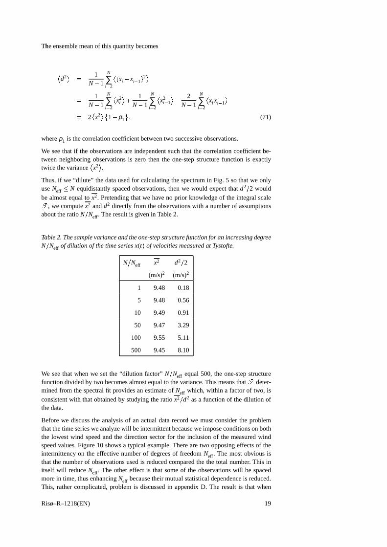
We seethat if the observationsareindependentsuchthat the correlationcoefficient be-tweenneighboringobservationsis zero then the one-stepstructurefunction is exactlytwice thevarianceg x2 h .Thus,if we “dilute” thedatausedfor calculatingthespectrumin Fig. 5 sothatwe onlyuseNeff Ó N equidistantlyspacedobservations,thenwe would expectthatd2 ? 2 would

bealmostequalto x2. Pretendingthatwe have no prior knowledgeof the integral scale� , we computex2 andd2 directly from theobservationswith a numberof assumptionsabouttheratioN ? Neff . Theresultis givenin Table2.

Table2.Thesamplevarianceandtheone-stepstructurefunctionfor anincreasingdegreeN ? Neff of dilution of thetimeseriesx � t of velocitiesmeasuredat Tystofte.

N ? Neff x2 d2 ? 2(m/s)2 (m/s)2

1 9.48 0.18

5 9.48 0.56

10 9.49 0.91

50 9.47 3.29

100 9.55 5.11

500 9.45 8.10

We seethat whenwe setthe “dilution factor” N ? Neff equal500, the one-stepstructurefunctiondividedby two becomesalmostequalto thevariance.Thismeansthat � deter-minedfrom thespectralfit providesanestimateof Neff which, within a factorof two, is

consistentwith thatobtainedby studyingtheratio x2 ? d2 asa functionof thedilution ofthedata.

Beforewe discussthe analysisof an actualdatarecordwe mustconsiderthe problemthatthetimeseriesweanalyzewill beintermittentbecauseweimposeconditionsonboththe lowestwind speedandthe directionsectorfor the inclusionof the measuredwindspeedvalues.Figure10 shows a typical example.Therearetwo opposingeffectsof theintermittency on the effective numberof degreesof freedomNeff . The mostobvious isthat thenumberof observationsusedis reducedcomparedthe the total number. This initself will reduceNeff . The othereffect is that someof the observationswill be spacedmorein time, thusenhancingNeff becausetheirmutualstatisticaldependenceis reduced.This, rathercomplicated,problemis discussedin appendixD. The result is that when

Risø–R–1218(EN) 19

the� total observationtime T is muchlargerthanthe integral time scale � thentheerrorvariance,i.e. theensemblevarianceof theintermittentlysampledmeanof x � t , becomes

σ2 A x B � 2 e x2 f �T F|||G |||H 1 � σ2χ ?¶e χ f 2

1 � η �σ2

χ � 1 � 2σ2χ I |||J|||K (72)

where e χ f andσ2χ arethe ensemblemeanandvarianceof the time seriesχ � t which is

onewhenthesignalx � t is fulfilling theinclusioncriteriaandzerootherwise,andwhereη is theaveragerateof changefrom χ � t � 1 to χ � t � 0.

By comparing(72) with (68) we seethat σ2 A x B is the usualerror variancefor the en-tire time serienswith a correctionfactor. Insteadof the lower equationin (67) whichessentiallystatesNeff ? N � ∆t ?m� 2 � we have

Neff

N� ∆t

2 � > F|||G |||H 1 � σ2χ ?me χ f 2

1 � η �σ2

χ � 1 � 2σ2χ I |||J|||K � 1 � (73)

4 Data Analysis

Thedata-analysisprocessis hereillustratedin acasewhereall theanemometersareRisøanemometersof thetypeshown in Fig. 1.

It is ageneralexperiencewith cupanemometersthatbelow acertain,anemometer-dependentwind speedthecalibrationceasesto belinear. In fact,theminimumwind speedat whichananemometerstartsrotationneednotbethesameatwhichit stopswhenthewind speedis decreasing.For mostcup anemometersthe wind speedbelow which thesecomplica-tionsareimportantis about1 m/s.Herewe choosea minimum3 m/swind speed.Thisdecisionis alsoinfluencedby the fact that in the wind tunnelswherereferencecalibra-tionsarecarriedout, thelowestwind speedis setto about4 m/s.We have alsochosenamaximumwind speedof 16 m/s,equalto thatusedin wind-tunnelcalibration.This lastchoiceis of little consequencebecausesuchhighwind speedsarequiteuncommonat theRisøcalibrationsite(Figs.2 and3).

In theperiodfrom themorningof June13 throughthemorningof July 11,2000we hadaratherlongperiodwith wind comingfrom west,overwater. The10wind-speedrecordsareshown in Fig. 7.

TheanemometerP300in positionRef1 wasusedasreference.Thisanemometerhasbeenwind-tunnelcalibratedby WINDTEST KWK GmbH (KWK in the following) in Ham-burg. Thefollowing linearrelationbetweenthewind speedU andthepulsefrequency f0in Hz wasobtained:

U � A0 > f0 � B0 (74)

whereA0� 0 � 61602m andB0

� 0 � 255m/s.

The cup anemometersP470.. .P477in the test positionswere also first calibratedbyKWK andthis gaveustheopportunityto comparethesecalibrationswith thoseobtained

20 Risø–R–1218(EN)

ÔÖÕ�×�Ø)Ù]Ú ÔÖÕ�×�ØÜÛ�Ý ÔÖÕ�×�ØÜÛßÞ Ô�Õ�àâá¬Ý�ã ÔÖÕ�à á�ÙÖÙä ÙåÍÙæ�زçèÙé ÙêëÙêoÛé Ûæ�زçpÛå�Ûä Û

ìpã�ÞÖÞìpã�Þ�íìîÚÖÝÖÝìpã�Þ�ïìpã�Þrãìpã�Þ�Úìpã�Þ�Ûìpãðï�ñìpã�ÞðÙìpã�Þ�Ý

Figure 7. Records of 10-minuteaveragesof the raw anemometersignalsfrom the cali-bration period fromJune13, 2000,10:45until July 11, 2000,10:05.Signalvaluescor-respondingto 3 m/sor lessareexcluded.Thiscorrespondsto 74%of thedata.Therangein each of the10 records is 0–1024.To the left are shownthepositionnamesandto theright theanemometercodenames.

from theboommeasurements(Fig.7) by comparingtheirsignalswith thesignalfrom thereferenceanemometerP300.

Thetechniquewasto fit theraw dataloggersignalsof theeight testanemometersto theraw referencesignalaccordingto themethoddescribedin section3. Convertingtherawsignalsto meanfrequenciesby multiplying by 32 anddividing by 600s (seesection2),wedeterminea andb in theequation

f0� a > f � b (75)

wherethefrequency f pertainsto thereferenceanemometer.

Thecalibrationexpressionfor thetestanemometeris

U � A > f � B (76)

and,sincethetestanemometerandthereferenceanemometersupposedlyhave beenex-posedto thesamewind history, wehave

A > f � B_ A0 > f0 � B0� A0 � a > f � b � B0 (77)

which implies

A � aA0 (78)

and

B � B0 � bA0 � (79)

First we selecteddatain 30� sectorsaround-60� , -30� , 0� , 30� , and60� . The result isshown in Fig. 8.

By inspectingFig. 8, weseethattheboomcalibrationsarein reasonableagreementwiththe wind-tunnelcalibrationswhen the wind comesfrom west in a broad150� sector.

Risø–R–1218(EN) 21

ò ó ô õ òò ó ô õ öò ó ô ÷ òò ó ô ÷ öò ó ô ø ò ùûúÏü ý þ ý úÏÿ������Îù�����ò ó ÷ ò òò ó ÷ ÷ òò ó ÷ � òò ó ÷ ô òò ó ÷ òò ó ø ò ò ��� ò � ô ò � � ø ò � ò � � ø ò � � ô ò � � � ò �

� � � � �� � � � �� � � � �� � � � �� � � � � ����� � � ��!#"%$'&��)(*�+-,

� � � � �� � � � �� � � . �� � � � �� � � / �� � � � �

0�1 � 2 � � 2 0 � � 2 � 2 3 � � 2 3 � � 2 3 1 � 2

4 5 6 7 44 5 6 7 84 5 6 9 44 5 6 9 84 5 6 : 4 ;�<= > ? > <@BADC�EF;�G�H�C�I

4 5 9 4 44 5 9 9 44 5 9 J 44 5 9 6 44 5 9 K 44 5 : 4 4

L�M 4 N 6 4 N L : 4 N 4 N O : 4 N O 6 4 N O M 4 N

P Q R S PP Q R S TP Q R U PP Q R U TP Q R V P W�X�Y Z [ Z X\#]_^�`FW)ab�c'd

P Q U P PP Q U U PP Q U e PP Q U R PP Q U f PP Q V P P

g�h P i R P i g V P i P i j V P i j R P i j h P i

k l m n kk l m n ok l m p kk l m p ok l m q k r�s�t u v u sw#xzy-{Fr)|}-|�~

k l p k kk l p p kk l p � kk l p m kk l p � kk l q k k

��� k � m k � � q k � k � � q k � � m k � � � k �

� � � � �� � � � �� � � � �� � � � �� � � � � ���� � � � ��B���-�F���������

� � � � �� � � � �� � � � �� � � � �� � � � �� � � � �

��� � � � � � � � � � � � � � � � � � � � � � � �

�   ¡ ¢ ��   ¡ ¢ £�   ¡ ¤ ��   ¡ ¤ £�   ¡ ¥ � ¦�§�¨ © ª © §�«#¬D­�®�¦)¯°±�²

�   ¤ � ��   ¤ ¤ ��   ¤ ³ ��   ¤ ¡ ��   ¤ ´ ��   ¥ � �

µ�¶ � · ¡ � · µ ¥ � · � · ¸ ¥ � · ¸ ¡ � · ¸ ¶ � ·

¹ º » ¼ ¹¹ º » ¼ ½¹ º » ¾ ¹¹ º » ¾ ½¹ º » ¿ ¹ À�ÁÂ Ã Ä Ã ÁÅ�ÆÈÇ-ÉFÀ�ÊËË�Ì

¹ º ¾ ¹ ¹¹ º ¾ ¾ ¹¹ º ¾ Í ¹¹ º ¾ » ¹¹ º ¾ Î ¹¹ º ¿ ¹ ¹

Ï�Ð ¹ Ñ » ¹ Ñ Ï ¿ ¹ Ñ ¹ Ñ Ò ¿ ¹ Ñ Ò » ¹ Ñ Ò Ð ¹ Ñ

Figure 8. Comparisonbetweenwind-tunnelcalibrationsand boomcalibrations.Thesewind-speeddata are divided into five different 30� direction sectors. The anemometerP300in positionRef1 is usedasreferencefor P470.. .P477. There is oneframefor eachof theseanemometers where the uppersubframepertainsto the slopeA and the lowerto theoffsetB. Theeightanemometers,P470.. .P477, havebeenwind-tunnelcalibratedon thesameday, June14,2000,andtheresultis shownasthreehorizontallinesindicat-ing the meanin the middlewhile the other two are the mean � onestandard deviation(68%confidencelimits). Theresultsfromthe boomcalibrationswith P300as referenceare shownas pointswith standard deviations for each directionsector. This referenceanemometerhasbeencalibratedin thesamewind tunnel,but on March 1, 2000.

However, the valuesof A in particularseemto fall below the wind-tunnelvalues.Thistendency could be causedby the fact that the eight testanemometersare wind-tunnelcalibratedon anotherdatethanthereferenceanemometer. We have testedif this shouldbethecasebyusingtheanemometerP475in positionC1asreference.Theresultisshownin Fig. 9. The tendency for A to be a little too small seemsto have disappeared(exceptfor P300now considereda testanemometer),but otherwisethe degreeof consistencybetweenboomcalibrationandwind-tunnelcalibrationappearsto be the sameaswhenP300is thereference.

Beingslightly cautious,wewill usedatafrom thesector0� � 45� in thefollowing.Figure10 shows how muchof the datais usedin the intercalibrationin oneparticularcase.Italsogivesanindicationof thedistributionanddurationof periodswhereχ � t is one.Thetotal time is 51% so that e χ f � 0 � 51 andσ2

χ� 0 � 25. The averagerateof changefrom

χ � t � 1 to χ � t � 0 is η � 2 � 4 d� 1. As shown in the previous section,thesedataareimportantfor determiningthestatisticaluncertaintyof thecalibrationparameters.

At thispoint it seemsnaturalto testwhethertheflow aroundaparticularcupanemometeris influencedby theneighborinstrumentson theboomfrom which it is separatedby thedistance0.75m. If theflow mustbeconsidereddisturbedwe would of courseexpectthedisturbanceto bemostpronouncedwhenthewind directionis far from beingperpendic-ular to theboom.To investigatethisproblemwecomparedaspecialsetof data,recordedin the period from August8, 2000until August28, 2000. In this period the positionsA2, B2, C2,andD2 wereunoccupiedwhereasRisøanemometerswereoccupying for alltheotherwere6 positions.Justasin thefirst measuringperiodin June-July, 2000,P458

22 Risø–R–1218(EN)

Ó Ô Õ Ö ÓÓ Ô Õ Ö ×Ó Ô Õ Ø ÓÓ Ô Õ Ø ×Ó Ô Õ Ù Ó Ú�ÛÜ Ý Þ Ý Ûß�à�á�âFÚ�ãäå�æ

Ó Ô Ø Ó ÓÓ Ô Ø Ø ÓÓ Ô Ø ç ÓÓ Ô Ø Õ ÓÓ Ô Ø è ÓÓ Ô Ù Ó Ó

é�ê Ó ë Õ Ó ë é Ù Ó ë Ó ë ì Ù Ó ë ì Õ Ó ë ì ê Ó ë

í î ï ð íí î ï ð ñí î ï ò íí î ï ò ñí î ï ó í ô�õ�ö ÷ ø ÷ õ�ù#ú%û'ü�ô)ýþ�ÿ��

í î ò í íí î ò ò íí î ò � íí î ò ï íí î ò � íí î ó í í

��� í � ï í � � ó í � í � � ó í � � ï í � � � í �

� � � � � � � � � � ����� � � � ����������� ��!"��#

� � � � $ � � � % �

&�' ( � ( & � ( ( ) � ( ) � ( ) ' (

* + , - ** + , - .* + , / ** + , / .* + , 0 * 1�2"3 4 5 4 2�687:9�;�1=<�>"?A@

* + / * ** + / / ** + / B ** + / , ** + / C ** + 0 * *

D�E * F , * F D 0 * F * F G 0 * F G , * F G E * F

H I J K HH I J K LH I J M HH I J M LH I J N H O�P"Q R S R P�T8UWV�X�O=Y�Z�Y�[

H I M H HH I M M HH I M \ HH I M J HH I M ] HH I N H H

^�_ H ` J H ` ^ N H ` H ` a N H ` a J H ` a _ H `

b c d e bb c d e fb c d g bb c d g fb c d h b i�j"k l m l j�n�oqpsrut"v�i=w"x�x�y

b c g b bb c g g bb c g z bb c g d bb c g { bb c h b b

|�} b ~ d b ~ | h b ~ b ~ � h b ~ � d b ~ � } b ~

� � � � �� � � � �� � � � �� � � � �� � � � � ���"� � � � ���8���"���=�������

� � � � �� � � � �� � � � �� � � � �� � � � �� � � � �

��� � � � � � � � � � � � � � � � � � � � � � � �

� � � � �� � � � �� � � � �� � � � �� � �   � ¡�¢�£ ¤ ¥ ¤ ¢�¦¨§ª©�«�¡ ¬�­�­�®

� � � � �� � � � �� � � ¯ �� � � � �� � � ° �� �   � �

±�² � ³ � � ³ ±   � ³ � ³ ´   � ³ ´ � � ³ ´ ² � ³

Figure9. SameasFig. 8, but with P475in positionC1 asreference.

µ·¶¨¸¨¹»ºq¼ µ·¶¨¸¨¹¾½À¿ µ·¶¨¸¨¹¾½WÁ µÀ¶¨ÂsÃÄ¿ÀÅ µ·¶¨Â Ãƺ·ºÇ ºÈɺ

Ê˹ÍÌÎºÏ ºÐѺÐÒ½Ï ½

Ê˹ÍÌÓ½ÈË½Ç ½

ÔÓŪÁ·ÁÔÓŪÁ:ÕÔÖ¼·¿·¿ÔÓŪÁÀ×ÔÓŪÁ�ÅÔÓŪÁ:¼ÔÓŪÁÀ½ÔÓÅØ×ÀÙÔÓŪÁغÔÓŪÁ:¿

Figure10.Recordsof 10-minuteaveragesof therawanemometersignalsin thedirectionsector0� � 45� fromthecalibrationperiodfromJune13,2000,10:45until July 11,2000,10:05.Signalvaluescorrespondingto 3 m/sor lessare excluded.Now51%of thedatafulfill thespeedanddirectionselectioncriteria.

andP300occupiedpositionsRef 2 andRef 1, respectively, but now the distancefromP458to the nearestanemometerin positionD1 was2.25 m (seeFig. 3). The resultofthecomparisonbetweenP458andthereferenceanemometerP300is shown in Fig. 11,whereboththefirst datasetwith all positionsoccupiedandthelastsetof datafrom Au-gustareused.If therewereno influenceon theflow from thedisturbancefrom neighboranemometers,bothconstantsA andB shouldbethesamein thetwo instruments.Theseconstantsareshown with their68%confidencelimits and,apparently, thevaluesof A aremorein agreementthanthevaluesof B. We see,however, thatthedependenceof thedis-agreementon wind directionis not pronounced.Using datafrom a 90� directionsectorcenteredaround0� , we find A � 0 � 6196� 0 � 0026m andB � 0 � 2442� 0 � 0104m/s fortheJunedataandA � 0 � 6175� 0 � 0040m andB � 0 � 2703� 0 � 0106m/sfor thoseof Au-

Risø–R–1218(EN) 23

gust.Ú Applying theso-calledZ-testfor two samplemeansto bethesame(Kanji 1999)atα � 5%,wefind thatZ � � 0 � 45for A andZ � 2 � 5 for B. Theα � 0 � 05limit for rejectionis Z � 1 � 96 sowe concludethat thecalibrationoffsetB is influencedby flow distortionfrom neighborinstrumentswhereaswe shouldnot rejectthatgainA is thesamewhetherit hasacloseneighborinstrumentor not.Whenthewind speedis morethanafew metersper secondthe accuracy of the gain is muchmoreimportantthanthe offset for reliablewind-speedmeasurements.In otherwords,thesystematicerroronB, whichmayamountto about0.02m/s,canin mostsituationsbeneglected.

ÛWÜ ÝWÞ Û

ÛWÜ ÝWÞ=ß

ÛWÜ Ý�àqÛ

ÛWÜ Ý�à�ß

ÛWÜ Ýqá�Û

âäã�å¾æ

çéèÓêªë�ì¨ë�èîíðïòñôóöõø÷ÒçöùÎúüûþý

ÛWÜ àuÛ�ÛÛWÜ àqàqÛÛWÜ àÍÿ:ÛÛWÜ àuÝ�ÛÛWÜ à���ÛÛWÜ áqÛ�Û

��� Û�� Ý�Û � � á�Û�� Û � � á�Û � � Ý�Û � � � Û �� ã å�� æ

Figure 11. Comparisonbetweencalibrationsof cupanemometerP458in positionRef2whenall boompositionsare occupied(period June2000)and whenpositionsA2, B2,C2,andD2 areempty, i.e. whenP458hasnocloseneighbors(August2000).In theupperframethevaluesof A fromtheJuneperiodare larger thanthosepertainingto theAugustperiod,exceptwhenthecenterdirectionis � 60� . For thevaluesof B it is justtheopposite.The68%confidencelimits are shownat each point.

5 Conclusion

It hasnow beendemonstratedhow it is possibleto simultaneouslycalibrateseveralcupanemometersin openair with asingleanemometerasthereference.It requiresthatall theanemometers,includingthe reference,areexposedto thesamewind flow. To guaranteethis, caremustbe taken that theanemometersdo not interferewith eachotherandthat,in general,the upstreamconditionsshouldlook the samefor all the anemometers.TheRisøcalibrationfacility is,asdescribedin section2,aboomwith 10anemometermounts,erectedparallelto thewestcoastof RoskildeFjord andwith a several-kilometerfetchofwatersurfacein a broaddirectionsectortowardswest.

Comparedto wind-tunnelcalibration,thereareadvantagesanddisadvantages.

Obviously it is advantageousto be ableto calibratemany anemometerssimultaneouslyat low labor cost.In particularwhenthe anemometersare later to be usedfor accuratecomparisonof wind fieldsat differentlocations,i.e. alonga verticalmastin caseswherereliablewindprofilesarerequired.Anotherbonusis thatnew cupanemometerscanbeop-

24 Risø–R–1218(EN)

erated� in thefield beforethey aredeployedfor realfield measurements:acupanemometerneedssometime,typically onemonth,to be“brokenin” if anew rotorwith new bearingshasbeeninstalled.

Onedisadvantageis that themethodobviously doesnot provide anabsolutecalibrationwith referenceto a certifiedwind tunnel.Sucha calibrationis often requiredby windturbinemanufacturesandownersfor themto beableto settleif a particularwind turbinehasproducedtheexpectedelectricenergy. Anotherdisadvantageis that it maytake verylong time to obtainacalibrationbecausetherearelimits to bothdirectionandmagnitudeof thefreewind.

In the analysisof datafrom the testfacility we found it naturalto useorthogonalmeansquarefitting insteadof the usual linear fitting with one independentand one depen-dentvariable.This is sobecausethesignalsfrom all theinstruments,includingreferenceanemometers,arealmostequal.Section3 andtheappendicesB, C,andD containaratherdetaileddiscussionof thefitting procedureandthestatisticalsignificanceof the results.Oneitem of particularimportanceis that, in contrastto measurementsin wind tunnels,consecutive setsof datacannotbeconsideredstatisticallyindependent.In fact,the timescale(or memory)of ten-minutewind speedaveragesis shown to beabout20 hours.Inprinciplethis meansthatdatasetsmustbeseparatedin timemorethanabout40hourstobeconsideredstatisticallyindependent.

We have testedwhetherthe flow arounda particularanemometeris disturbedby thepresenceof theneighboranemometersandwe foundthat thecalibrationgainA appearsunaffectedwhereastheoffsetB seemsinfluencedin asystematicway. However, whenthewind speedis morethana few meterspersecondtheoffset,beingitself about0.2m/s,isof little importance.

Thequestionis if thefield calibrationis really preferableto wind tunnelcalibration.Tocalibratea cupanemometerwill in the lastcasetypically take abouthalf anhour. Theremight be a slight overheadfor settingup a calibrationstand,but altogethera setof 10anemometerscan be calibratedin the courseof one day. It can also be arguedthat agenerallyapproved calibrationcanbe obtainedonly by useof a certifiedwind tunnel.Theproblemwith this is of coursethat thereareseveralcertifiedwind tunnelsandthatthey do not alwaysgive thesamecalibrationfor thesameanemometer.

This is probablysobecausethereferencewind speedin a tunnelis determinedby mea-suringthevery smallpressuredifferences(about0.1HPa or less)from a Pitot tube.Thepressuredetectoris temperaturesensitive andoutmostcaremustbetakenby monitoringthetemperatureof theair in thewind tunnel.Eventhenthereseemsto beproblemsandto illustratethis point we have hadtheeightcupanemometerscalibratednot only in theKWK wind tunnel,but alsoin thewind tunnelof SvendOleHansenAps(SOH).Thefirstcalibrationtook placeon June14,2000,thesecondon August23,2000.Thecalibrationresultsaresummarizedin Table3. We seethat for all eight anemometersthe measuredgainsA arelarger in the SOH tunnelwhereasthe oppositeis the casefor the offsetsB.In fact, the differencesof the last areall between0.1 m/s and0.2 m/s. Judgingby theconfidencelimits, thedifferencesdonot seemto bewithin thestatisticalvariability.

To illustratehow muchthe differencein the two calibrationsinfluencethe actualmea-suredwind speeds,we have plottedthe velocity differencewith 68% confidencelimitsovera rangeof about0 to 20m/sfor oneof thecupanemometers,P475.This is shown inFig. 12.We seethat thecalibrationsagreewithin � 0 � 05 m/sin a wind speedrangefromabout7 m/sto about12 m/s.This relatively pooragreementin calibrationsseemssome-whatdisappointingin view of thehigh quality of theanemometersin termsof long-termstabilityof thecalibration.

Perhapsthebestsolutionto obtainreliablecalibrationsof cupanemometersis to modify

Risø–R–1218(EN) 25

Table3. Comparisonbetweenwind tunnelcalibrationsat KWK andSOH. ThegainsAandtheoffsetsB are givenwith 68%confidencelimits.

KWK SOH

A (m) B (m/s) A (m) B (m/s)

P470 0.6213 � 0.0007 0.247 � 0.012 0.6299 � 0.0007 0.118 � 0.011

P471 0.6213 � 0.0008 0.253 � 0.013 0.6299 � 0.0007 0.109 � 0.010

P472 0.6214 � 0.0005 0.244 � 0.008 0.6289 � 0.0007 0.152 � 0.011

P473 0.6230 � 0.0007 0.231 � 0.010 0.6303 � 0.0011 0.121 � 0.016

P474 0.6223 � 0.0005 0.248 � 0.008 0.6284 � 0.0009 0.144 � 0.014

P475 0.6203 � 0.0005 0.263 � 0.008 0.6282 � 0.0011 0.138 � 0.016

P476 0.6218 � 0.0005 0.265 � 0.010 0.6298 � 0.0012 0.148 � 0.017

P477 0.6218 � 0.0005 0.262 � 0.008 0.6288 � 0.0011 0.157 � 0.016

thewind-tunnelcalibrationprocedureby usinga“standard”cupanemometer, ratherthana Pitot-tube,asreferenceanemometer. ���������

� �������

� ��! "$#%

&(')+*)�'*

,-*,.'&.*&/')+*)�'*'

0 '213)�*0 '213)!'0 '214'.*'214'/'5 '216'-*5 '217)�'5 '217)+*

Figure12.Comparisonbetweencalibrationsof cupanemometerP475in theKWK windtunneland theSOHwind tunnel.Thesolid, thick line is thewind speedcalculatedwiththeKWK calibrationparametersminusthewindspeedcalculatedwith theSOHcalibra-tion asfunctionof frequencyf . Thecorrespondingwind speed,usingtheaverage of thetwo calibrationsis shownalong the upperabscissa.Thedashedlines indicatethe 68%confidencelines.

26 Risø–R–1218(EN)

A Regressionwith Curvature

We wantto investigatetheorthogonalregressionto a curvewhich is “almost” straight.

We use(2) in thegeneralizedform

r � r0 � θ t � θ � (A1)

Theparameterθ is the lengthof thechordfrom a referencepoint r0� x0i � y0 j on the

curveto thecurvepoint r � θ � xi � yj.

Theexpression(5) for theunit vectort maystill beusedif weconsiderα afunctionof θ .

From FG H x

y

I JK � FG H x0 � θ cos� α � θ y0 � θ sin� α � θ I JK (A2)

weobtain

θ 2 � � x � x0 2 ��� y � y0 2 � (A3)

We consideronly smallcurvaturesandassumetheapproximation

cos� α � θ i cosα0 � α k0θ sinα0

sin� α � θ ] i sinα0 � α k0θ cosα0 (A4)

whereα0� α � 0 is thedirectionof thetangentin thereferencepoint r0 andα k0 � α k � 0

its derivative.

This impliesthat(A2) canbewritten

x � x0� θ cosα0 � α k0θ 2sinα0

y � y0� θ sinα0 � α k0θ 2cosα0 (A5)

or, by using(A3) to eliminateθ 2,� x � x0 � α k0 8 � x � x0 2 ��� y � y0 2 9 sinα0� θ cosα0� y � y0 p� α k0 8 � x � x0 2 ��� y � y0 2 9 cosα0� θ sinα0 � (A6)

Multiplying thefirst equationby sinα0 andthesecondby cosα0 andsubtracting,we getthefollowing equationfor thecurve` x � x0 � sinα0

2α k0 c 2 � ` y � y0 � cosα0

2α k0 c 2 � ` 12α k0 c 2 (A7)

which is the equationfor a circle with radiusequalto 1?m\ 2α k0 \ andcenterin the point� x0 � sinα0 ?¶� 2α k0 � y0 � cosα0 ?¶� 2α k0 � .It is now very simpleto determinethe perpendicular(signed)distancedi from a pointwith the coordinates� xi yi to the curve. It is simply the distanceto the centerof thecircleminustheradius.

28 Risø–R–1218(EN)

di� : ` xi � x0 � sinα0

2α k0 c 2 � ` yi � y0 � cosα0

2α k0 c 2 � 12 \α k0 \i 1

2 \α k0 \ < 1 � 2α k0 8 � xi � x0 sinα0 � � yi � y0 cosα09� 2α k02 8 � xi � x0 2 �T� yi � y0 2 9� 2α k02 8 � xi � x0 sinα0 � � yi � y0 cosα09 2 � 1 P� α k0\α k0 \<; � xi � x0 sinα0 � � yi � y0 cosα0� α k0 < � xi � x0 cosα0 �T� yi � y0 sinα0 = 2 = � (A8)

For N points � xi yi , i � 1 2 �]� � N wecalculatethedistancesdi to thecircleandminimize

φ � 1N

N

∑i � 1

d2i (A9)

to obtainthe bestfit to the circle (A7) in termsof the parametersx0, y0, α0, andα k0 ofwhich only threeareindependent.

At thispointweassumethatwecandetermineα k0 with sufficientaccuracy by first findingx0, y0, andα0 underthe assumptionthat the line is straightandthencalculatingα k0 bysolving ∂φ ? ∂α k0 � 0 with respectto α k0, with x0, y0, andα0 assumedknown. Herewehave thefreedomto set � x0 y0 � � 0 0 andconsequentlyobtainthesolution

α k0 � � � xsinα0 � ycosα0 � xcosα0 � ysinα0 � 2� xcosα0 � ysinα0 � 4 � (A10)

We cannow studyhow theslopea � a � θ � tan� α varies.We have

a � tan� α0 � α k0θ � i tanα0 � � 1 � tan2α0 � α k0θ � (A11)

To comparethechangeof a with θ with a itself wemustselectarange∆θ of θ . Wehavechosenthesquarerootof samplevarianceof θ asthis range:

∆θ � t θ 2 � b x2 � y2 � (A12)

Thecorrespondingchangein a is then

∆a _ a � tanα0� � 1 � tan2α0 � α k0∆θ i � 1 � a2 α k0∆θ � (A13)

B Monte Carlo Simulations

We have madeMonteCarlosimulationsin orderto establisha numericalverificationof(49),andalsoto studythequalityof theapproximationbehindthis formula,for aselectedsequenceof ρ0-values.

Risø–R–1218(EN) 29

To@ carryout this taskweneededaprocedurefor producingstandardizednormalvariates,assumingthata supplyof independent,uniformly distributed(pseudo)randomnumbersξi > U � 0 1 areavailable from the computer. Sucha methodwasdesignedby Box &Muller (1958)whoproposedto generatepairsof independentvaluesby therecipe

x � � � 2lnξ1 1̂ 2cos� 2πξ2 (B1)

and

y � � � 2lnξ1 1̂ 2sin� 2πξ2 � (B2)

It is easyto verify that

x > N � 0 1� (B3)

y > N � 0 1� (B4)

andthat

Cov � x y� � 0 � (B5)

First we notethat(B1) producespositive andnegativenumberswith equalprobabilities.We maythereforeconsiderpositivevaluesonly andthusreplace(B1) by

x � � � 2lnξ1 1̂ 2cos� 12πξ2 � uv� (B6)

Let f , g, h bedensityfunctionsfor x, u, v, respectively, andF , G correspondingdistribu-tion functions.Thenwehave

F � x � � 1

0h � v G M x

vO dv (B7)

or

f � x � � 1

0h � v g M x

vO dv

v� (B8)

Now

g � u �@???? dξ1

du???? � ue� 1

2u2(B9)

and

h � v �A???? dξ2

dv???? � 2

π1B

1 � v2(B10)

Thus

f � x � 2π

� 1

0

x

v2B

1 � v2exp `�� 1

2x2

v2 c dv� (B11)

This integralcanbeevaluatedby substitutingv � x? B x2 � u2. Theresultis

f � x � 21B2π

e� 12x2

(B12)

30 Risø–R–1218(EN)

which{ is thedoubleof thenormaldensity, asit shouldbe.Now (B4) followsimmediatelyfrom (B3), and(B5) followsby symmetryreasonsC .

Whatwe neednext is a methodfor generatingcorrelatedpairsof normaldeviates,sam-pled for a given correlationcoefficient ρ0. We first generate� x y asin (B1) and(B2).Thenwe take` xk

yk c � ` cB

1 � c2B1 � c2 c

c ` xyc (B13)

wherec is a parameterin theinterval � � 1 1� . From(B13) wefind thecovariancematrix

D � ` cB

1 � c2B1 � c2 c

c 2 � ` 1 2cB

1 � c2

2cB

1 � c2 1c � (B14)

We mustrequire

2c t 1 � c2 � ρ0 (B15)

or

c2 � 1 � b 1 � ρ20

2� (B16)

Now we are in a position to simulatepairs � xi yi , i � 1 �]� � N suchthat xi > N � 0 1 ,yi > N � 0 1 , andCov � xi yi � � ρ0. Our choiceV � xi � � V � yi � � 1 is naturalin view of ourknowledgethatV � xi �¶i V � yi � . Next we compute

s2x� x2

i s2y� y2

i sxy� xiyi (B17)

and,accordingto (17)and(18),

δ � 12

ln V s2x

s2y W (B18)

ε � 12

ln V s2xs2

y

s2xy W (B19)

and finally a by (20). We repeatthe simulationfor j � 1 � �]� M, eachtime recordinga � a j . In this way we cancomputethesamplevariances2 � a of a. Finally we comparetheresultwith (49).

Weusedafixednumberof M � 100repetitions,andwith thisweransimulationsfor N �10,100,1000,and10000.For eachN we took ρ0

� 0.9,0.99,and0.999.Theresultsareshown in thefollowing tables:

N � 10

ρ0 2 � 1 � ρ0 ? N s2 � a0.9 2 � 00� 10� 2 2 � 74� 10� 2

0.99 2 � 00� 10� 3 3 � 23� 10� 3

0.999 2 � 00� 10� 4 2 � 30� 10� 4

Risø–R–1218(EN) 31

N � 100

ρ0 2 � 1 � ρ0 ? N s2 � a0.9 2 � 00� 10� 3 2 � 94� 10� 3

0.99 2 � 00� 10� 4 1 � 75� 10� 4

0.999 2 � 00� 10� 5 1 � 96� 10� 5

N � 1000

ρ0 2 � 1 � ρ0 ? N s2 � a0.9 2 � 00� 10� 4 2 � 80� 10� 4

0.99 2 � 00� 10� 5 2 � 05� 10� 5

0.999 2 � 00� 10� 6 2 � 17� 10� 6

N � 10000

ρ0 2 � 1 � ρ0 ? N s2 � a0.9 2 � 00� 10� 5 2 � 44� 10� 5

0.99 2 � 00� 10� 6 2 � 21� 10� 6

0.999 2 � 00� 10� 7 2 � 09� 10� 7

Not surprisingly, theagreementis bestfor ρ0 closeto 1.

C DiscreteSampling

Wearehereconsideringtheerrorvariancein thecasewhereweincludethelimit ∆t ¹ � .

We replace(61)and(62)by

x � 1N

N � 1

∑D � 0

x � � ∆t (C1)

and

σ2 A x B � l � x � e xf 2 n� 1N

N � 1

∑DFE � 0

1N

N � 1

∑D7E E � 0

gQ� x ��� k ∆t p� e xf � � x � � k k ∆t q� e xf � h� e x2 f 1N

N � 1

∑DFE � 0

1N

N � 1

∑DFE E � 0

ρ � � � k k � � k ∆t � (C2)

wherewehaveused(60) for thelaststep.

By comparing(C2)and(62),weseethatthelastis apoorapproximationto thefirst when∆t ¹Ò� sincethe smallest,non-zeroincrementin the summation(C2) is thenso largethatthecorrespondingchangein ρ � τ cannotbeconsideredsmall.

Applying theFouriertransform

ρ � τ � ∞�� ∞

S� f eqπ i f τd f (C3)

32 Risø–R–1218(EN)

to (C2),we get

σ2 A x B � e x2 f 1N

N � 1

∑D E � 0

1N

N � 1

∑D E E � 0

∞�� ∞

S� f exp � 2π i f ∆t � � k k � � k � d f� e x2 f ∞�� ∞

S� f d f????? 1N N � 1

∑D � 0

e2π i f ∆tD ?????

2

� e x2 f ∞�� ∞

HN � f S� f d f (C4)

where

HN � f � sin2 � π f N∆t N2sin2 � π f ∆t � (C5)

We areconcernedwith situationswhereN � T ? ∆t ¹ 1 in which limit HN � f becomesproportionalto aso-calleddelta-comb,whichis asumof equidistantlyspaceddeltafunc-tions:

HN � f · limN G ∞

HN � f � 1T

∞

∑m� � ∞

δ M f � m∆tO � (C6)

We thusobtainthegeneralexpression

σ2 A x B � e x2 fT

∞

∑m� � ∞

∞�� ∞

S� f δ M f � m∆tO d f � e x2 f

T

∞

∑m� � ∞

S M m∆tO (C7)

valid whenN ¹ 1.

In thelimit ∆t Ñ 0 thereis only onetermin thesum(C7) andwe get

σ2 A x B � e x2 f S� 0T (C8)

which is identicalto (69).

In theotherlimit, ∆t Ñ ∞, thesumbecomesanintegral:

σ2 A x B � e x2 fT

∞

∑m� � ∞

S M m∆tO δm�������H 1� e x2 f ∆t

T

∞

∑m� � ∞

S M m∆tO δ M m

∆tO

· e x2 f ∆tT

∞�� ∞

S� f d f� ��� �� 1

� e x2 fN� (C9)

We seethatnow Neff becomesequalto N asexpected.

Risø–R–1218(EN) 33

D Intermittent Sampling

In orderto analyzeintermittenttimeseries,wefirst consideranuninterruptedtimeseriesx0 � t from whichwe canobtainanintermittenttime seriesby

x � t � χ � t x0 � t Ö (D1)

wherethetwo-valuedindex functionχ � t canattainthevaluesoneandzero.

Let usconsidera moregeneralsystemwhich canonly exist in two states,anupperstateanda lower. Theprobabilitythatthesystemflips from onestateto theotherat leastoncein a given,small time interval is proportionalto theduration∆t of this interval. Let thisprobability be k∆t, wherek is a constant.Consequently, the probability that the systemhasnot changedbecomes1 � k∆t. Theprobability that thesystemhasnot changedstatein thefixed,finite time T � N∆t becomes

p � T � limN G ∞

L � 1 � k∆t N P � limN G ∞

R ` 1 � kTNc N U � e� kT � (D2)

Thesystemwe want to discusshasin generaltwo differentdecayconstantskI andk� ,characterizingflips from the upperto the lower and from the lower to the upperstate,respectively.

We considera systemat start time t � 0 andseekthe probability that the systemis inthesamestateastheoriginal oneat time t J 0,in otherwordsthat it hasflippedanevennumberof times.Let usstartwith thesystemin theupperstate.Thentheprobabilityforno flips is

PI/I0 � t � e� kK t � (D3)

Theprobabilityfor thesystemto bein thelowerstateat time t afteroneflip is

PI �1 � t � t�

0

e� kK t1 kI dt1e� kL�M t � t1 N � (D4)

Continuingthis process,the probability for beingbackin the upperstateafter just twoflips becomes

PI/I2 � t � t�

0

e� kK t1 kI dt1

t�t1

e� kL+M t2 � t1 N k� dt2PI(I0 � t � t2 � (D5)

We thusobtainthefollowing recursionrelationfor n O 1

PI/I2n � t � t�

0

e� kK t1 kI dt1

t�t1

e� kL+M t2 � t1 N k� dt2PI(I2n � 2 � t � t2 � kI k� t�

0

e� M kK � kL N t1 dt1

t�t1

e� kL t2 PI/I2n � 2 � t � t2 dt2� kI k�

kI � k� t�0

L e� kL t1 � e� kK t1 P PI/I2n � 2 � t � t1 dt1 (D6)

34 Risø–R–1218(EN)

where{ wehaveappliedintegrationby partsto obtainthelastexpression.

We maynow sumup all theseprobabilities:

PI/I � t _ ∞

∑n� 0

PI(I2n � t � e� kK t � ∞

∑n� 1

PI/I2n � t � (D7)

Inserting(D6) we getthefollowing integralequationfor PI(I � t :

PI/I � t � e� kK t � kI k�

kI � k� t�0

L e� kL t1 � e� kK t1 P PI(I � t � t1 dt1 � (D8)

Thisis aVolterraintegralequationof thesecondkind andit caneasilybesolvedby meansof Laplacetransforms.Writing P I(I � s _RQÒA PI/I � t B we obtain

P I/I � s � 1s � kI � kI k�

kI � k� P I/I � s y 1s � k� � 1

s � kIEz (D9)

with thesolution

P I/I � s � 1kI � k� y k�

s� kI

s � kI � k� z � (D10)

Transformingbackto time domainyields

PI/I � t � k� � kI e� M kK I kL N t

kI�� k� � (D11)

This result could have beenobtainedin a simplerway, aspointedout by Jakob Mann(2000,privatecommunication),namelyasthesolutionto thefirst-orderdifferentialequa-tion

dPI(I

dt� � kI P

I(I � t � k� � 1 � PI(I � t � � (D12)

However, we have adoptedthe methoddescribedherebecauseit hasprovideda usefulinsightin the‘mechanismof flips’.

Theprobability that thesystemis in the lower statewhenit is at theupperat t � 0 is ofcourse

PI � � t � 1 � P

I/I � t � kI � kI e� M kK I kL N tkI®� k� � (D13)

Similarly, we canstartin thelower stateandthecorrespondingprobabilitiesP�p� � t andP� I � t areobtainedby interchangingkI andk� in (D11)and(D13).

We maynow proceedto determinetheexpectednumberof doubleflips in thetime t. Apriori we would expectthis numberto beproportionalto t, but we needa rigorousproofthatthis is indeedthecase.Let usagainconsiderthesystemin theupperpositionat timet � 0. Thenthe numberN

I � t of doubleflips canbe expressedin termsof PI(I � t as

follows:

NI � t � ∞

∑n� 0

nPI(I2n � t � P

I/I2 � t � ∞

∑n� 2

nPI(I2n � t � (D14)

Risø–R–1218(EN) 35

InsertingS (D6) we get

NI � t � P

I/I2 � t �kI k�

kI � k� t�0

L e� kL M t � θ N � e� kK M t � θ N P dθ∞

∑n� 2

nPI/I2n � 2 � θ � (D15)

Thesumin theintegral canberearrangedasfollows

∞

∑n� 2

nPI(I2n � 2 � θ � ∞

∑n� 2

� n � 1 PI/I2n � 2 � θ � ∞

∑n� 2

PI/I2n � 2 � θ � N

I � θ � PI(I � θ p� P

I(I0 � θ (D16)

and,applyingthisexpression,(D15)becomes

NI � t � kI k�

kI � k� t�0

L e� kL+M t � θ N � e� kK+M t � θ N P < N I � θ � PI/I � θ = dθ (D17)

wherewehaveused(D6) for n � 1. AgainwetaketheLaplacetransform,use(D10),andsolve for T I � s _UQÒA N I � t B . Thus

T I � s � kI k� � kI � k� � kI � k� 3 y 1s � 1

s � kI � k� z� kI k�� kI®� k� 2 y k�s2 � kI� s � kIÂ� k� 2 z (D18)

with theinversetransform

NI � t � kI k� � kI � k� � kI�� k� 3 L 1 � e� M kK I kL N t P� kI k�� kI�� k� 2 L k� t � kI te� M kK I kL N t P (D19)

Similarly, the averagenumberof doubleflips if the systemstartsin the lower statebe-comes

N �ë� t � kI k� � k� � kI � kI�� k� 3 L 1 � e� M kK I kL N t P� kI k�� kI � k� 2 L kI t � k� te� M kK I kL N t P � (D20)

The total expectednumberN � t of doubleflips, irrespective of the initial statecanbedeterminedfrom (D19)and(D20)by addingthem,afterweightingthemwith theapriori

36 Risø–R–1218(EN)

probabilities@ Π I andΠ I for being in the upperstateandthe lower state,respectively.SinceΠ I k � � Π � k � they become

РI � k�kI�� k� (D21)

and

Π � � kIkI � k� � (D22)

Theresultis

N � t � k�kI®� k� N

I � t � kIkI®� k� N �Ü� t � kI k�� kI®� k� 3 L � k2I®� k2� � t � 2kI k� te� M kK I kL N t P� kI k� � kI � k� 2� kIÂ� k� 4 L 1 � e� M kK I kL N t P � (D23)

Weseethatonly for largevaluesof t cantheaveragenumberof doubleflips beconsideredproportionalto t:

N � t · kI k� � k2I � k2� � t� kIÂ� k� 3 � kI®� k� t ¹ 1 � (D24)

Whent is smallwe get

N � t · 12

kI k� t2 � kI®� k� t ¸ 1 � (D25)

We now assignthe value1 to the upperstateand0 to the lower. In order to relatethedecayconstantskI andk� to observablequantitieswe calculatetheensemblemeanandensemblevarianceof thecorresponding,stationarytimeseriesχ � t . We havee χ � t f � Π

I > 1 � � > 0 � k�kI�� k� (D26)

and

σ2χ _Ðe]� χ � t p� e χ � t f 2 f ��� Π

I > 1 � e χ � t f 2 f � kI k�� kI®� k� 2 � (D27)

We mayuseobservationof χ � t overa long time to determinekI andk� in termsof σ2χ

andthelong-termrateof doubleflips

η � kI k� � k2I�� k2� �� kI � k� 3 � (D28)

Solving the two equations(D27) and (D28) with respectto kI and k� , we get, if weassumethatk� J kI :

kV � η

2σ2χ M 1 � 2σ2

χO L 1 W b 1 � 4σ2

χ P � (D29)

Risø–R–1218(EN) 37

The{ auto-covariancefunctionfor χ � t is

Rχ � t2 � t1 _ gQ� χ � t1 p� e χ f � � χ � t2 q� e χ f � h� g χ � t1 χ � t2 h � e χ f 2 � Π I PI(I � t2 � t1 p� e χ f 2� kI k�� kI � k� 2 e� M kK I kL N � t2 � t1 � � (D30)

We now definethetotal time Θ duringwhich χ � t is equalto oneduringtheobservationtimeT by

Θ � T � T�0

χ � t dt � (D31)

Thisdefinitionimmediatelyimpliesthate Θ � T f � k� T

kI�� k� � (D32)

Thevariancebecomes

σ2Θ � T _ l � Θ � T p� e Θ � T f 2 n� X T�

0

� χ � t1 p� e χ f � dt1

T�0

� χ � t2 p� e χ f � dt2 Y� T�0

dt1

T�0

dt2Rχ � t2 � t1 � kI k�� kI�� k� 2 T�0

dt1

T�0

dt2e� M kK I kL N � t2 � t1 �� 2kI k� T� kI � k� 3 R 1 � 1 � e� M kK I kL N T� kI � k� T U � (D33)

Since

σΘ � T e Θ � T f · : 2kI�? k�� kI�� k� T (D34)

when � kIÂ� k� T ¹ 1, wefind thatΘ � T , givenby (D31), in this limit is agoodapprox-imationto theensembleaveragee Θ � T f .Thesamplemeanof x � t � χ � t x0 � t asgivenin (D1 now becomes

x � 1Θ

T�0

x � t dt � 1Θ

T�0

χ � t x0 � t dt � (D35)

38 Risø–R–1218(EN)

AlthoughZ this is certainlynot truein generalwe assume—inorderto capturein a simpleway the essenceof the consequencesof conditionalsampling—χ � t andx0 � t uncorre-lated.

Consequently, theensemblemeanof x becomes

e xf � X 1Θ

T�0

χ � t x0 � t dt Y� T�0

vχ � t Θw g x0 � t h dt � g x0

ha� 0 � (D36)

For thevarianceof x weget

σ2 A x B � g � x � e xf 2 h �AX 1Θ

T�0

χ � t1 x0 � t1 dt11Θ

T�0

χ � t2 x0 � t2 dt2 Y· 1

Θ

T�0

dt11Θ

T�0

dt2 e x20 f ρ0 � t2 � t1 e χ � t1 χ � t2 f� e x2

0 fΘ

T�0

dt11Θ

T�0

dt2 ρ0 � t2 � t1 < e χ f 2 � Rχ � t2 � t1 = (D37)

whereρ0 � t is theautocorrelationfunctionfor x0 � t .Combiningthis equationwith (D26), (D27), (D30),and(D32),weseethat

σ2 A x B � e x20 f

T

T�0

dt11T

T�0

dt2 ρ0 � t2 � t1 y 1 � kIk� e� M kK I kL N � t2 � t1 � z � (D38)

Assuming

ρ0 � t � e��� t � ^�� (D39)

theerrorvariancebecomesin thelimit where � kI®� k� T ¹ 1 aswell asT ?Q� ¹ 1

σ2 A x B � 2 e x20 f �T y 1 � kIÍ? k�

1 ��� kI � k� � z� 2 e x20 f �T F|||G |||H 1 � σ2

χ ?¶e χ f 21 � η �

σ2χ � 1 � 2σ2

χ I |||J|||K (D40)

wheretheparametersin the lastexpression,definedby (D26), (D27) and(D28), canbederiveddirectly from themeasuredrecordχ � t .Risø–R–1218(EN) 39

Acknowledgements

We would like to expressourgratitudeto ourcolleaguesJanNielsenfor helpingwith theillustrationof thecalibrationfacility, JakobMannfor discussingandproviding assistancein theevaluationof theinfluenceonthestatisticsof dataintermittence,LarsLandberg forhis encouragement.

40 Risø–R–1218(EN)

References

Box, G. E. P. & Muller, M. E. (1958),‘A noteon thegenerationof randomnormaldevi-ates’,Ann.Math.Statist.29, 610–611.

Brazier, C. E. (1914),Recherchesexpérimentalessur les moulenetsanémometrique,in‘Ann. Bur. Centr. Météorol.France’,pp.157–300.

Kanji, G. K. (1999),100 StatisticalTests, SagePublications,London,ThousandOaks,andNew Delhi.

Kristensen,L. (1994),Cups,propsandvanes,TechnicalReportR–766(EN),RisøNa-tionalLaboratory.

Kristensen,L. (1998),‘Cup anemometerbehavior in turbulentenvironments’,J. Atmos.Ocean.Technol.15, 5–17.

Kristensen,L. (1999),‘The perennialcupanemometer’,Wind Energy2, 59–75.

Kristensen,L. (2000),‘Measuringhigher-ordermomentswith a cupanemometer’,J. At-mos.Ocean.Technol.17, 1139–1148.

Kristensen,L., Rathmann,O.& Hansen,S.O. (1999),Extremewindsin Denmark,Tech-nicalReportR–1068(EN),RisøNationalLaboratory.

Lenschow, D. H., Mann, J. & Kristensen,L. (1994), ‘How long is long enoughwhenmeasuringfluxesandotherturbulencestatistics’,J. Atmos.Ocean.Technol.11, 661–673.

Middleton,W. E.K. (1969),Inventionof Meteorological Instruments, TheJohnsHopkinsPress,Baltimore,MD.

Patterson,J. (1926),‘The cupanemometer’,Trans.Roy. Soc.Canada,Ser. III 20, 1–54.

Wyngaard,J. C. (1981),‘Cup, propeller, vane,andsonicanemometersin turbulencere-search’,Ann.Rev. Fluid Mech. 13, 399–423.

Risø–R–1218(EN) 41

Bibliographic[ Data Sheet Risø–R–1218(EN)

Title andauthor(s)

FieldCalibrationof CupAnemometers

Leif Kristensen,GunnarJensen,Arent Hansen,andPeterKirkegaard

ISBN

87–550–2772–5;87–550–2773–3(Internet)

ISSN

0106–2840

Dept.or group

Departmentof Wind Energy

Date

January23,2001

Groupsown reg. number(s)

1105016–00

Project/contractNo.

1105-16-00

Sponsorship

Pages

42

Tables

3

Illustrations

12

References

12

Abstract(Max. 2000char.)

An outdoorcalibrationfacility for cupanemometers,wherethesignalsfrom10anemome-tersof which at leastoneis a referencecanbecanberecordedsimultaneously, hasbeenestablished.Theresultsarediscussedwith specialemphasisonthestatisticalsignificanceof thecalibrationexpressions.It is concludedthatthemethodhastheadvantagethatmanyanemometerscanbecalibratedaccuratelywith a minimumof work andcost.Theobvi-ousdisadvantageis that thecalibrationof a setof anemometersmaytake morethanonemonth in order to have wind speedscovering a sufficiently large magnituderangein awind directionsectorwherewe canbesurethattheinstrumentsareexposedto identical,simultaneouswind flows.Anothermainconclusionis thatstatisticaluncertaintymustbecarefully evaluatedsincethe individual 10 minutewind-speedaveragesarenot statisti-cally independent.

DescriptorsINIS/EDB

WIND; VELOCITY; ANEMOMETER;CALIBRATION; FIELD TESTS;DATA ANALYSIS

Availableonrequestfrom InformationServiceDepartment,RisøNationalLaboratory(Afdelingenfor Informationsservice,ForskningscenterRisø),P.O. Box 49,DK–4000Roskilde,Denmark.Phone+4546 7740 04,Fax +454677 4013,E-mail infserv@risoe.dk