feedforward neural networks: an …catalogimages.wiley.com/images/db/pdf/0471349119.01.pdf · 1...

1FEEDFORWARD

NEURAL NETWORKS: AN INTRODUCTION

Simon Haykin

1

A neural network is a massively parallel distributed processor thathas a natural propensity for storing experiential knowledge andmaking it available for use. It resembles the brain in two respects(Haykin 1998):

1. Knowledge is acquired by the network through a learningprocess.

2. Interconnection strengths known as synaptic weights are usedto store the knowledge.

Basically, learning is a process by which the free parameters (i.e.,synaptic weights and bias levels) of a neural network are adaptedthrough a continuing process of stimulation by the environment inwhich the network is embedded. The type of learning is determinedby the manner in which the parameter changes take place.In a generalsense, the learning process may be classified as follows:

• Learning with a teacher, also referred to as supervised learning• Learning without a teacher, also referred to as unsupervised

learning

1.1 SUPERVISED LEARNING

This form of learning assumes the availability of a labeled (i.e.,ground-truthed) set of training data made up of N input—outputexamples:

(1.1)

where xi = input vector of ith exampledi = desired (target) response of ith example, assumed to be

scalar for convenience of presentationN = sample size

Given the training sample T, the requirement is to compute the freeparameters of the neural network so that the actual output yi of theneural network due to xi is close enough to di for all i in a statisticalsense. For example, we may use the mean-square error

(1.2)

as the index of performance to be minimized.

1.1.1 Multilayer Perceptrons and Back-Propagation Learning

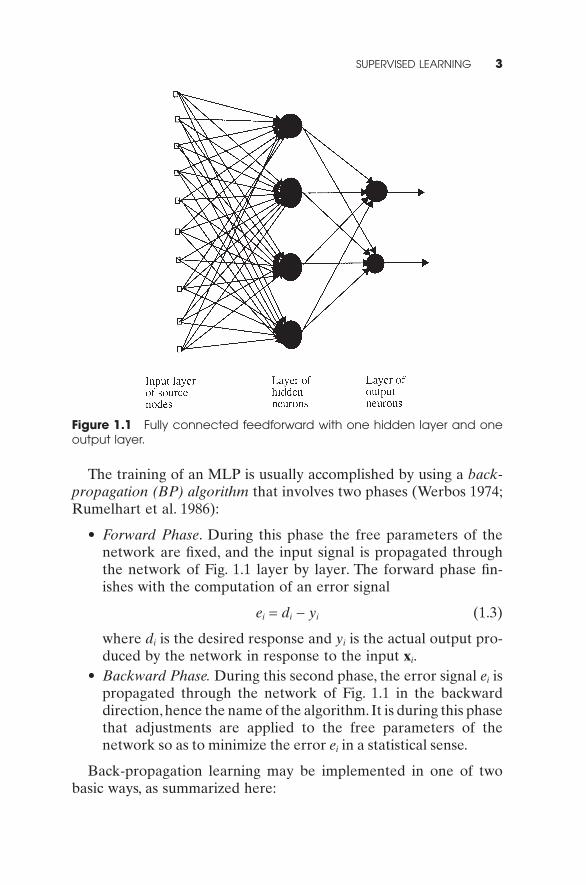
The back-propagation algorithm has emerged as the workhorse forthe design of a special class of layered feedforward networks knownas multilayer perceptrons (MLP). As shown in Fig. 1.1, a multilayerperceptron has an input layer of source nodes and an output layerof neurons (i.e., computation nodes); these two layers connect thenetwork to the outside world. In addition to these two layers,the multilayer perceptron usually has one or more layers of hiddenneurons, which are so called because these neurons are not directlyaccessible. The hidden neurons extract important features containedin the input data.

E n

Nd yi i

i

N

( ) = -( )=Â1 2

1

T di i i

N= ( ){ } =x , 1

2 FEEDFORWARD NEURAL NETWORKS: AN INTRODUCTION

The training of an MLP is usually accomplished by using a back-propagation (BP) algorithm that involves two phases (Werbos 1974;Rumelhart et al. 1986):

• Forward Phase. During this phase the free parameters of thenetwork are fixed, and the input signal is propagated throughthe network of Fig. 1.1 layer by layer. The forward phase fin-ishes with the computation of an error signal

ei = di - yi (1.3)

where di is the desired response and yi is the actual output pro-duced by the network in response to the input xi.

• Backward Phase. During this second phase, the error signal ei ispropagated through the network of Fig. 1.1 in the backwarddirection,hence the name of the algorithm. It is during this phasethat adjustments are applied to the free parameters of thenetwork so as to minimize the error ei in a statistical sense.

Back-propagation learning may be implemented in one of twobasic ways, as summarized here:

SUPERVISED LEARNING 3

Figure 1.1 Fully connected feedforward with one hidden layer and oneoutput layer.

1. Sequential mode (also referred to as the on-line mode or sto-chastic mode): In this mode of BP learning, adjustments aremade to the free parameters of the network on an example-by-example basis. The sequential mode is best suited for patternclassification.

2. Batch mode: In this second mode of BP learning, adjustmentsare made to the free parameters of the network on an epoch-by-epoch basis, where each epoch consists of the entire set oftraining examples. The batch mode is best suited for nonlinearregression.

The back-propagation learning algorithm is simple to implement andcomputationally efficient in that its complexity is linear in the synap-tic weights of the network. However, a major limitation of the algo-rithm is that it does not always converge and can be excruciatinglyslow, particularly when we have to deal with a difficult learning taskthat requires the use of a large network.

We may try to make back-propagation learning perform better byinvoking the following list of heuristics:

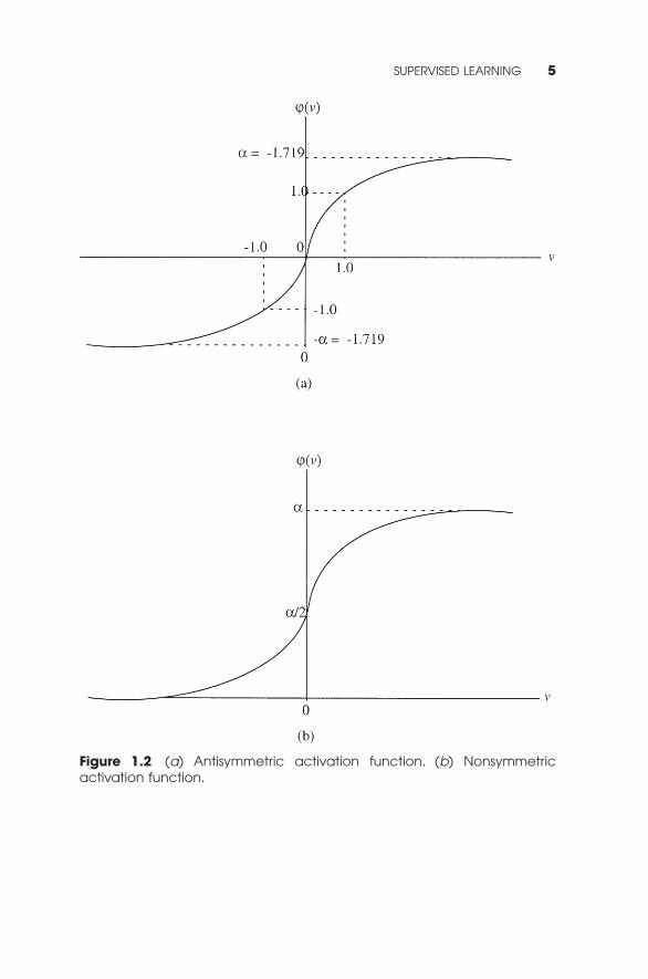
• Use neurons with antisymmetric activation functions (e.g.,hyperbolic tangent function) in preference to nonsymmetricactivation functions (e.g., logistic function). Figure 1.2 showsexamples of these two forms of activation functions.

• Shuffle the training examples after the presentation of eachepoch; an epoch involves the presentation of the entire set oftraining examples to the network.

• Follow an easy-to-learn example with a difficult one.• Preprocess the input data so as to remove the mean and decor-

relate the data.• Arrange for the neurons in the different layers to learn at essen-

tially the same rate. This may be attained by assigning a learn-ing rate parameter to neurons in the last layers that is smallerthan those at the front end.

• Incorporate prior information into the network design when-ever it is available.

One other heuristic that deserves to be mentioned relates to thesize of the training set,N, for a pattern classification task.Given a mul-tilayer perceptron with a total number of synaptic weights includingbias levels, denoted by W, a rule of thumb for selecting N is



Figure 1.2 (a) Antisymmetric activation function. (b) Nonsymmetric activation function.

(1.4)

where O denotes “the order of,” and e denotes the fraction of clas-sification errors permitted on test data. For example, with an errorof 10% the number of training examples needed should be about 10times the number of synaptic weights in the network.

Supposing that we have chosen a multilayer perceptron to betrained with the back-propagation algorithm, how do we determinewhen it is “best” to stop the training session? How do we select thesize of individual hidden layers of the MLP? The answers to theseimportant questions may be gotten though the use of a statisticaltechnique known as cross-validation, which proceeds as follows(Haykin 1999):

• The set of training examples is split into two parts:• Estimation subset used for training of the model• Validation subset used for evaluating the model performance

• The network is finally tuned by using the entire set of trainingexamples and then tested on test data not seen before.

1.1.2 Radial-Basis Function Networks

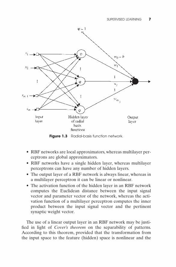
Another popular layered feedforward network is the radial-basisfunction (RBF) network which has important universal approxima-tion properties (Park and Sandberg 1993), and whose structure isshown in Fig. 13. RBF networks use memory-based learning for theirdesign. Specifically, learning is viewed as a curve-fitting problem inhigh-dimensional space (Broomhead and Lowe 1989; Poggio andGirosi 1990):

1. Learning is equivalent to finding a surface in a multidimen-sional space that provides a best fit to the training data.

2. Generalization (i.e., response of the network to input data notseen before) is equivalent to the use of this multidimensionalsurface to interpolate the test data.

RBF networks differ from multilayer perceptrons in some funda-mental respects:

N O

W= ÊË

ˆ¯e


• RBF networks are local approximators, whereas multilayer per-ceptrons are global approximators.

• RBF networks have a single hidden layer, whereas multilayerperceptrons can have any number of hidden layers.

• The output layer of a RBF network is always linear, whereas ina multilayer perceptron it can be linear or nonlinear.

• The activation function of the hidden layer in an RBF networkcomputes the Euclidean distance between the input signalvector and parameter vector of the network, whereas the acti-vation function of a multilayer perceptron computes the innerproduct between the input signal vector and the pertinentsynaptic weight vector.

The use of a linear output layer in an RBF network may be justi-fied in light of Cover’s theorem on the separability of patterns.According to this theorem, provided that the transformation fromthe input space to the feature (hidden) space is nonlinear and the


Figure 1.3 Radial-basis function network.

dimensionality of the feature space is high compared to that of theinput (data) space, then there is a high likelihood that a nonsepara-ble pattern classification task in the input space is transformed intoa linearly separable one in the feature space.Another analytical basisfor the use of RBF networks (and multilayer perceptrons) in classi-fication problems is provided by the results in Chapter 2, where (asa special case) it is shown that a large family of classification prob-lems in �n can be solved using nonlinear static networks.

Design methods for RBF networks include the following:

1. Random selection of fixed centers (Broomhead and Lowe1998)

2. Self-organized selection of centers (Moody and Darken 1989)3. Supervised selection of centers (Poggio and Girosi 1990)4. Regularized interpolation exploiting the connection between

an RBF network and the Watson–Nadaraya regression kernel(Yee 1998).

1.2 UNSUPERVISED LEARNING

Turning next to unsupervised learning, adjustment of synapticweights may be carried through the use of neurobiological principlessuch as Hebbian learning and competitive learning. In this sectionwe will describe specific applications of these two approaches.

1.2.1 Principal Components Analysis

According to Hebb’s postulate of learning, the change in synapticweight Dwji of a neural network is defined by

Dwji = hxiyj (1.5)

where h = learning-rate parameterxi = input (presynaptic) signalyi = output (postsynaptic) signal

Principal component analysis (PCA) networks use a modified formof this self-organized learning rule. To begin with, consider a linearneuron designed to operate as a maximum eigenfilter; such a neuron is referred to as Oja’s neuron (Oja 1982). It is characterizedas follow:


(1.6)

where the term -hy2j wji is added to stabilize the learning process. As

the number of iterations approaches infinity, we find the following:

1. The synaptic weight vector of neuron j approaches the eigen-vector associated with the largest eigenvalue l max of the corre-lation matrix of the input vector (assumed to be of zero mean).

2. The variance of the output of neuron j approaches the largesteigenvalue l max.

The generalized Hebbian algorithm (GHA), due to Sanger (1989),is a straightforward generalization of Oja’s neuron for the extractionof any desired number of principal components.

1.2.2 Self-Organizing Maps

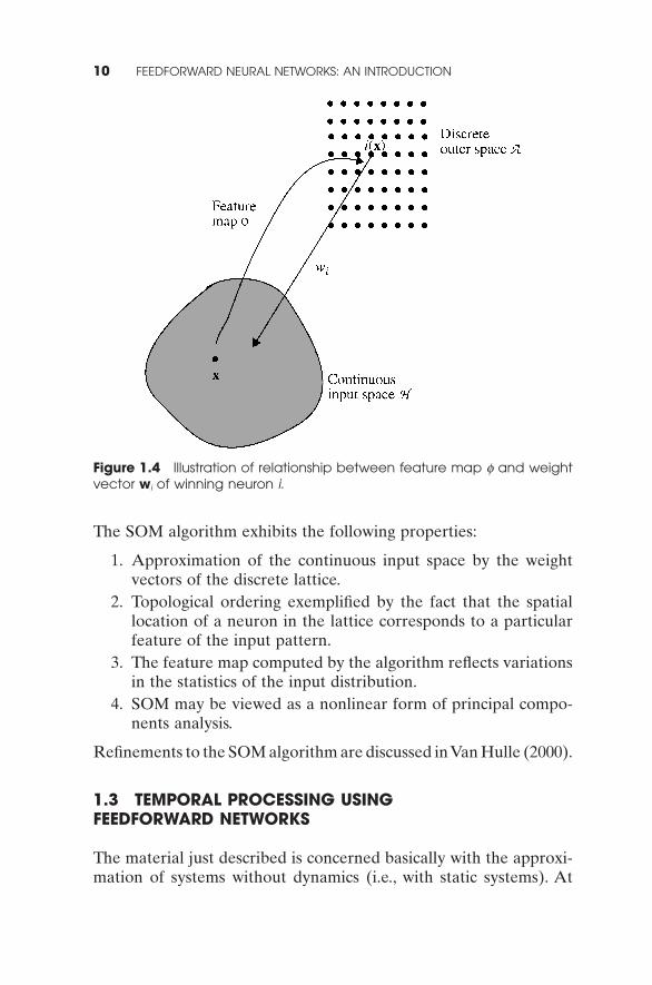
In a self-organizing map (SOM), due to Kohonen (1997), the neuronsare placed at the nodes of a lattice, and they become selectivelytuned to various input patterns (vectors) in the course of a compet-itive learning process. The process is characterized by the formationof a topographic map in which the spatial locations (i.e., coordinates)of the neurons in the lattice correspond to intrinsic features of theinput patterns. Figure 1.4 illustrates the basic idea of a self-organiz-ing map, assuming the use of a two-dimensional lattice of neurons asthe network structure.

In reality, the SOM belongs to the class of vector-coding algo-rithms (Luttrell, 1989). That is, a fixed number of codewords areplaced into a higher-dimensional input space, thereby facilitatingdata compression.

An integral feature of the SOM algorithm is the neighborhoodfunction centered around a neuron that wins the competitiveprocess. The neighborhood function starts by enclosing the entirelattice initially and is then allowed to shrink gradually until it encom-passes the winning neuron.

The algorithm exhibits two distinct phases in its operation:

1. Ordering phase, during which the topological ordering of theweight vectors takes place

2. Convergence phase, during which the computational map is finetuned

Dw y x y wji j i j ji= -( )h

UNSUPERVISED LEARNING 9

The SOM algorithm exhibits the following properties:

1. Approximation of the continuous input space by the weightvectors of the discrete lattice.

2. Topological ordering exemplified by the fact that the spatiallocation of a neuron in the lattice corresponds to a particularfeature of the input pattern.

3. The feature map computed by the algorithm reflects variationsin the statistics of the input distribution.

4. SOM may be viewed as a nonlinear form of principal compo-nents analysis.

Refinements to the SOM algorithm are discussed in Van Hulle (2000).

1.3 TEMPORAL PROCESSING USING FEEDFORWARD NETWORKS

The material just described is concerned basically with the approxi-mation of systems without dynamics (i.e., with static systems). At


Figure 1.4 Illustration of relationship between feature map f and weightvector wi of winning neuron i.

about the same time as the appearance of the early universal-approximation theorems for static neural networks there began(Sandberg 1991a) a corresponding study (see Chapter 2) of the neuralnetwork approximation of approximately-finite-memory maps andmyopic maps. It was found that large classes of these maps can be uni-formly approximated arbitrarily well by the maps of certain simplenonlinear structures using, for example, sigmoidal nonlinearities orradial basis functions. The approximating networks are two-stagestructures comprising a linear preprocessing stage followed by amemoryless nonlinear network. Much is now known about the prop-erties of these networks,and examples of these properties are given inthe following.

From another perspective, time is an essential dimension of learning. We may incorporate time into the design of a neuralnetwork implicitly or explicitly.A straightforward method of implicitrepresentation of time1 is to add a short-term memory structure inthe input layer of a static neural network (e.g., multilayer percep-tron).The resulting configuration is sometimes called a focused time-lagged feedforward network (TLFN).

The short-term memory structure may be implemented in one oftwo forms, as described here:

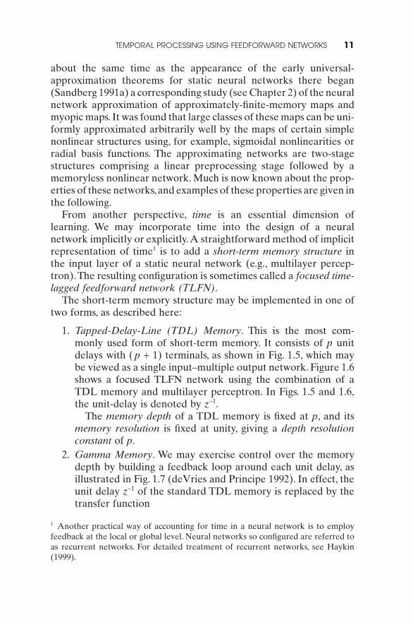
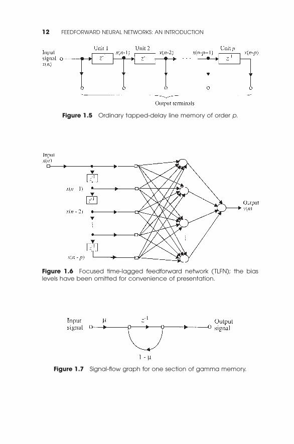
1. Tapped-Delay-Line (TDL) Memory. This is the most com-monly used form of short-term memory. It consists of p unitdelays with ( p + 1) terminals, as shown in Fig. 1.5, which maybe viewed as a single input–multiple output network. Figure 1.6shows a focused TLFN network using the combination of aTDL memory and multilayer perceptron. In Figs. 1.5 and 1.6,the unit-delay is denoted by z-1.

The memory depth of a TDL memory is fixed at p, and itsmemory resolution is fixed at unity, giving a depth resolutionconstant of p.

2. Gamma Memory. We may exercise control over the memorydepth by building a feedback loop around each unit delay, asillustrated in Fig. 1.7 (deVries and Principe 1992). In effect, theunit delay z-1 of the standard TDL memory is replaced by thetransfer function

TEMPORAL PROCESSING USING FEEDFORWARD NETWORKS 11

1 Another practical way of accounting for time in a neural network is to employfeedback at the local or global level. Neural networks so configured are referred toas recurrent networks. For detailed treatment of recurrent networks, see Haykin(1999).


Figure 1.5 Ordinary tapped-delay line memory of order p.

Figure 1.6 Focused time-lagged feedforward network (TLFN); the biaslevels have been omitted for convenience of presentation.

Figure 1.7 Signal-flow graph for one section of gamma memory.

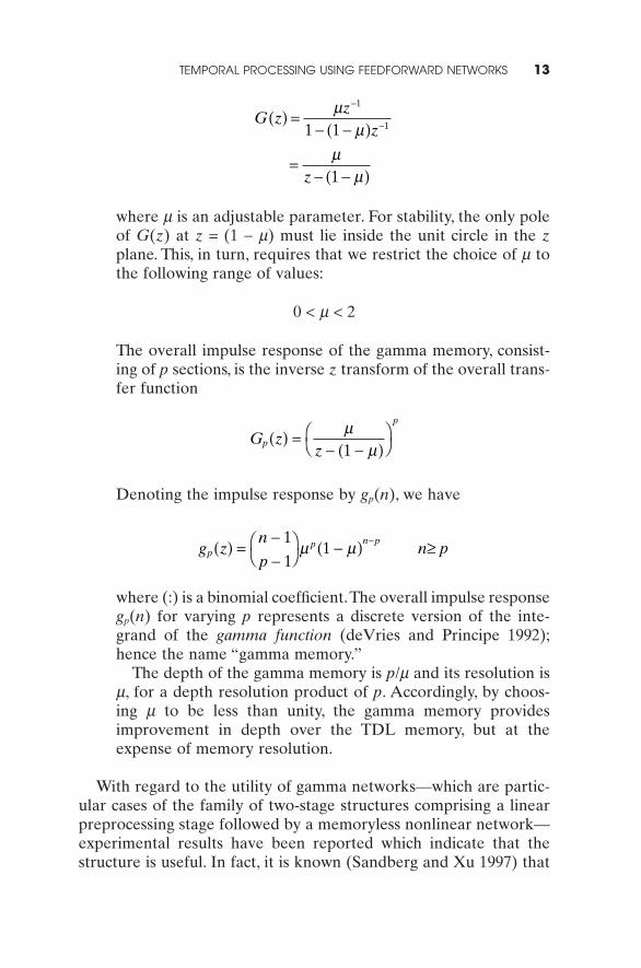
where m is an adjustable parameter. For stability, the only poleof G(z) at z = (1 - m) must lie inside the unit circle in the zplane. This, in turn, requires that we restrict the choice of m tothe following range of values:

0 < m < 2

The overall impulse response of the gamma memory, consist-ing of p sections, is the inverse z transform of the overall trans-fer function

Denoting the impulse response by gp(n), we have

where (:) is a binomial coefficient.The overall impulse responsegp(n) for varying p represents a discrete version of the inte-grand of the gamma function (deVries and Principe 1992);hence the name “gamma memory.”

The depth of the gamma memory is p/m and its resolution ism, for a depth resolution product of p. Accordingly, by choos-ing m to be less than unity, the gamma memory providesimprovement in depth over the TDL memory, but at theexpense of memory resolution.

With regard to the utility of gamma networks—which are partic-ular cases of the family of two-stage structures comprising a linearpreprocessing stage followed by a memoryless nonlinear network—experimental results have been reported which indicate that thestructure is useful. In fact, it is known (Sandberg and Xu 1997) that

g z

n

pn pp

p n p( ) =--

ÊË

ˆ¯ -( ) ≥-1

11m m

G z

zp

p

( ) =- -( )

ÊË

ˆ¯

mm1

G zz

z

z

( ) =- -( )

=- -( )

-

-

mm

mm

1

11 1

1

TEMPORAL PROCESSING USING FEEDFORWARD NETWORKS 13

for a large class of discrete-time dynamic system maps H, and forany choice of m in the interval (0, 1), there is a focused gammanetwork that approximates H uniformly arbitrarily well. It is knownthat tapped-delay-line networks (i.e., networks with m = 1) also havethe universal approximation property (Sandberg 1991b).

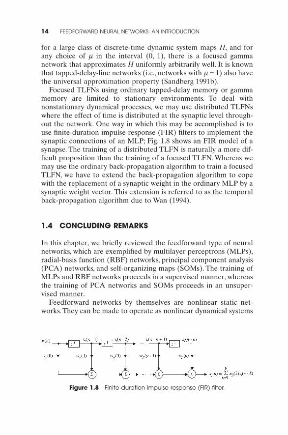
Focused TLFNs using ordinary tapped-delay memory or gammamemory are limited to stationary environments. To deal with nonstationary dynamical processes, we may use distributed TLFNswhere the effect of time is distributed at the synaptic level through-out the network. One way in which this may be accomplished is touse finite-duration impulse response (FIR) filters to implement thesynaptic connections of an MLP; Fig. 1.8 shows an FIR model of asynapse. The training of a distributed TLFN is naturally a more dif-ficult proposition than the training of a focused TLFN. Whereas wemay use the ordinary back-propagation algorithm to train a focusedTLFN, we have to extend the back-propagation algorithm to copewith the replacement of a synaptic weight in the ordinary MLP by asynaptic weight vector. This extension is referred to as the temporalback-propagation algorithm due to Wan (1994).

1.4 CONCLUDING REMARKS

In this chapter, we briefly reviewed the feedforward type of neuralnetworks, which are exemplified by multilayer perceptrons (MLPs),radial-basis function (RBF) networks, principal component analysis(PCA) networks, and self-organizing maps (SOMs). The training ofMLPs and RBF networks proceeds in a supervised manner, whereasthe training of PCA networks and SOMs proceeds in an unsuper-vised manner.

Feedforward networks by themselves are nonlinear static net-works. They can be made to operate as nonlinear dynamical systems


Figure 1.8 Finite-duration impulse response (FIR) filter.

by incorporating short-term memory into their input layer. Twoimportant examples of short-term memory are the standard tapped-delay-line and the gamma memory that provides control over attain-able memory depth. The attractive feature of nonlinear dynamicalsystems built in this way is that they are inherently stable.

BIBLIOGRAPHY

Anderson, J. A., 1995, Introduction to Neural Networks (Cambridge, MA:MIT Press).

Barlow, H. B., 1989, “Unsupervised learning,” Neural Computation, vol. 1,pp. 295–311.

Becker, S., and G. E. Hinton, 1982, “A self-organizing neural network thatdiscovers surfaces in random-dot stereograms,” Nature (London), vol.355, pp. 161–163.

Broomhead, D. S., and D. Lowe, 1988, “Multivariable functional inter-polation and adaptive networks,” Complex Systems, vol. 2, pp. 321–355.

Comon, P., 1994,“Independent component analysis:A new concept?” SignalProcessing, vol. 36, pp. 287–314.

deVries, B., and J. C. Principe, 1992, “The gamma model—A new neural model for temporal processing,” Neural Networks, vol. 4, pp.565–576.

Haykin, S., 1999, Neural Networks: A Comprehensive Foundation, 2nd ed.(Englewood Cliffs, NJ: Prentice-Hall).

Moody and Darken, 1989, “Fast learning in networks of locally-tuned pro-cessing unites,” Neural Computation, vol. 1, pp. 281–294.

Oja, E., 1982, “A simplified neuron model as a principal component ana-lyzer,” J. Math. Biol., vol. 15, pp. 267–273.

Park, J., and Sandberg, I. W., 1993, “Approximation and radial-basis func-tion networks,” Neural computation, vol. 5, pp. 305–316.

Poggio, T., and F. Girosi, 1990, “Networks for approximation and learning,”Proc. IEEE, vol. 78, pp. 1481–1497.

Rumelhart, D. E., G. E. Hinton, and R. J. Williams, 1986, “Learning internalrepresentations by error propagation,” in D. E. Rumelhart and J. L.McCleland, eds. (Cambridge, MA: MIT Press), vol. 1, Chapter 8.

Sandberg, I. W., 1991a, “Structure theorems for nonlinear systems,” Multi-dimensional Sys. Sig. Process. vol. 2, pp. 267–286. (Errata in 1992, vol. 3,p. 101.)

Sandberg, I. W., 1991b, “Approximation theorems for discrete-timesystems,” IEEE Trans. Circuits Sys. vol. 38, no. 5, pp. 564–566, May 1991.

BIBLIOGRAPHY 15

Sandberg, I. W., and Xu, L., 1997, “Uniform approximation and gamma net-works,” Neural Networks, vol. 10, pp. 781–784.

Van Hulle, M. M., 2000, Faithful Representations and Topographic Maps:From Distortion-to-Information-Based Self Organization (New York:Wiley).

Wan, E. A., 1994, “Time series prediction by using a connectionist networkwith internal delay lines,” in A. S. Weigend and N. A. Gershenfield, eds.,Time Series Prediction: Forecasting the Future and Understanding the Past(Reading, MA: Addison-Wesley), pp. 195–217.

Werbos, P. J., 1974, “Beyond regression: New tools for prediction and analy-sis in the behavioral sciences,” Ph.D. Thesis, Harvard University,Cambridge, MA.

Werbos, P. J., 1990, “Backpropagation through time: What it does and howto do it,” Proc. IEEE, vol. 78, pp. 1550–1560.

Yee, P. V., 1998, “Regularized radial basis function networks: Theory andapplications to probability estimation, classification, and time series pre-diction,” Ph.D. Thesis, McMaster University, Hamilton, Ontario.


feedforward neural networks: an …catalogimages.wiley.com/images/db/pdf/0471349119.01.pdf · 1...

Documents