faster joins, self-joins and multi-way joins using join indices
TRANSCRIPT

ELSEVIER Data & Knowledge Engineering 29 (1999) 179-200
I DATA & KNOWLEDGE ENGINEERING
Faster joins, self-joins and multi-way joins using join indices r . a 1 2
H u i L e l ' ' , K e n n e t h A . R o s s * ' b
alBM T.J. Watson Research Center, Route 134, Yorktown Heights, New York, NY 10598, USA bDepartment of Computer Science, Columbia University, New York, NY 10027, USA
Accepted 1 July 1998
A b s t r a c t
We propose a new algorithm, called Stripe-join, for performing a join given a join index. Stripe-join is inspired by an algorithm called 'Jive-join' developed by Li and Ross. Stripe-join makes a single sequential pass through each input relation, in addition to one pass through the join index and two passes through a set of temporary files that contain tuple identifiers but no input tuples. Stripe-join performs this efficiently even when the input relations are much larger than main memory, as long as the number of blocks in main memory is of the order of the square root of the number of blocks in the participating relations. Stripe-join is particularly efficient for self-joins. To our knowledge, Stripe-join is the first algorithm that, given a join index and a relation significantly larger than main memory, can perform a self-join with just a single pass over the input relation and without storing input tuples in intermediate files. Almost all the I/O is sequential, thus minimizing the impact of seek and rotational latency. The algorithm is resistant to data skew. It can also join multiple relations while still making only a single pass over each input relation. Using a detailed cost model, Stripe-join is analyzed and compared with competing algorithms. For large input relations, Stripe-join performs significantly better than Valduriez's algorithm and hash join algorithms. We demonstrate circumstances under which Stripe-join performs significantly better than Jive-join. Unlike Jive-join, Stripe-join makes no assumptions about the order of the join index. © 1999 Elsevier Science B.V. All rights reserved.
Keywords: Relational databases; Join; Query processing; Decision support systems
1. Introduction
Decision support systems promise significant added value to an organization's information resources. The basic challenge today is to develop efficient query processing techniques that can turn this promise into reality for a wide variety of potential users.The join operation of the relational database model is the fundamental operation that allows information from different relations to be
* Corresponding author. E-mail: [email protected] This work was performed while the author was at Columbia University; e-mail: [email protected]
2 This research was supported by a grant from the AT&T Foundation, by a David and Lucile Packard Foundation Fellowship in Science and Engineering, by a Sloan Foundation Fellowship, by NSF CISE award CDA-96-25374, and by an NSF Young Investigator award IRI-94-57613.
0169-023X/99/$ - see front matter © 1999 Elsevier Science B.V. All rights reserved. PII: S 0 1 6 9 - 0 2 3 X ( 9 8 ) 0 0 0 3 1-7

180 H. Lei, K.A. Ross / Data & Knowledge Engineering 29 (1999) 179-200
combined. Joins are typically expensive operations, particularly when the relations involved are substantially larger than main memory. Therefore, it is critical to implement joins in the most efficient way possible. A number of techniques have been developed to perform 'ad hoc' joins, i.e., joins performed without the benefit of additional data structures such as indices [3,4,6,10,15,18].
In this paper, we consider joins of relations for which there exists a pre-computed access structure, namely a join index [19]. A join index between two relations maintains pairs of identifiers of tuples that would match in case of a join. The join index may be maintained by the database system, and updated when tuples are inserted and deleted in the underlying relations. In situations where joins are taken often, the cost of doing this maintenance can be more than offset by the savings achieved in performing the join. A number of commercial decision support systems are rumored to be using join indexes [ 17].
In [19], Valduriez proposed and analyzed a join algorithm that uses the join index. The most important conclusion of that study was that, under many circumstances, having the join index allows one to compute the join significantly faster than the 'best' ad hoc methods such as Hybrid hash-join [6]. However, it was shown in [14,13] that Valduriez's algorithm utilizes a significant amount of repetitious I/O. Blocks are accessed often for only a small fraction of their tuples. The same block may be read multiple times on different passes within the algorithm.
In [14,13], Li and Ross proposed two algorithms that significantly improve upon Valduriez's algorithm. The algorithms are called 'Jive-join' and 'Slam-join.' The two algorithms are duals of one another, and have very similar performance. Jive-join range-partitions the tuple-ids of the second input relation, then processes each partition separately. Slam-join forms sorted runs of tuple-ids from the second input relation, then merges those runs.
The crucial virtue of both algorithms is that they make just a single read pass through each input relation under lenient memory requirements. Unlike hash-join algorithms, input tuples are not stored in intermediate files; intermediate files contain just short tuple identifiers. Other important features of those algorithms include: (a) Almost all of the I /O performed is sequential. (b) A block of an input relation is read if and only if it contains a record that participates in the join. (c), Skew does not adversely affect the performance. (d) One can join multiple relations, retaining the single-pass property of the inputs, by using multidimensional data structures.
In this paper, we propose a new algorithm that is similar to the Jive-join algorithm of [14,13]. Our , . . . . , 3
new algorithm, which we term :Stripe-join, has several important advantages over Jive-join: • Jive-join requires a fixed ordering of the join index. If the join index is not stored in such an
order, one would have to first sort it before applying Jive-join. There is no assumption made about the physical order of the join index in Stripe-join. Thus, Stripe-join can avoid this sorting step.
• Stripe-join is symmetric with respect to all relations. The join index is first processed, then all participating relations are processed in a symmetric fashion. Jive-join, on the other hand, treats one relation in particular as 'special' by reading it at the same time as the join index. The symmetry of Stripe-join has an important performance benefit: For joins in which a relation R appears more than once, Stripe-join can make a single pass through R to cover all of the instances of R in the join. In particular, self-joins can be performed with just one pass through the
3 'Stripe' is both an acronym (Symmetric Treatment of Relations that have a join Index and that are Particularly Extensive) and a phrase intended to allude to the vertically partitioned nature of the join result.

H. Lei, K.A. Ross / Data & Knowledge Engineering 29 (1999) 179-200 181
self-joined relation. We believe that the symmetry property also renders Stripe-join easily extensible to parallel architectures.
• Stripe-join delivers better performance under some circumstances, in particular when the cardinality of the join index is high.
Like Jive-join, Stripe-join uses a vertically partitioned data structure for the join result. (We do not
assume that the inputs are vertically partitioned.) Attributes from the first input relation are stored in a separate file from those of the second input relation, using transposed files [1]. Attributes that are common are placed arbitrarily in one of the two vertical fragments. There is a one-to-one correspondence between records in each vertical partition: The nth record in the first vertical fragment matches the nth record in the second. Such a representation has a negligible performance impact on processes that read the join result [14,13]. It is our understanding that vertical partitioning is being deployed in some current proprietary commercial database systems, including Sybase IQ and Red Brick.
Our main contributions include: • The proposal of a novel algorithm for joining relations using a join index. To our knowledge this
is the first algorithm that, given a join index and a relation significantly larger than main memory, can perform a self-join with just a single pass over the input relation and without storing input tuples in intermediate files.
• The analytic performance analysis of the algorithm using a detailed cost model, demonstrating efficient single-pass performance under lenient memory requirements.
• Analytic comparisons of our algorithms with other algorithms, demonstrating significant performance improvements under several conditions.
The structure of the paper is as follows. In Section 2 we discuss our assumptions and present the vertically partitioned data structure for the join result. In Section 3 we present our Stripe-join algorithm, which is then analyzed in Section 4. Section 5 compares our algorithms with other algorithms. Section 6 discusses various extensions of our algorithms. We conclude in Section 7.
2. B a c k g r o u n d
We consider an r-way join of r relations. (A conventional join has r = 2; while the most common type of join is probably a two-way join, the description of our algorithms is only slightly more complex in the r-way case, and so we simply present the r-way join algorithm directly.) The input relations to be joined are denoted by R 1 . . . . . R r. We assume for simplicity that a tuple-id for each input relation is simply the 'position' of the tuple within the relation (e.g., 1, 2 . . . . ). However, our algorithm applies for any sequential physical addressing scheme for which input relation records in one block have smaller tuple-id values than the records in the next block. Tuple-ids are used in the join index and in the intermediate results of our join algorithm.
A join index is the set of tuples (t~ . . . . . tr) of tuple-ids such that the tuple-ids t/ from R i refer to tuples that match according to the join condition. We shall treat the join index as a relation, and denote it by J. We do not assume that the join index is physically ordered by any attribute.
For simplicity, we shall assume that all of the attributes of each R i are required in the join result. The extension of our analysis to cases where fewer attributes are required is straightforward.

182 H. Lei, K.A. Ross / Data & Knowledge Engineering 29 (1999) 179-200
We do not assume that any indexes are available on the input relations. We also do not assume that either input relation is physically ordered by any attribute.
Following [9,8], we assume that separate disks are used to store: (a)join indices; (b) temporary files; (c) input relations, and (d) the output result. By using separate disks we avoid unnecessary disk seeks between accesses. The input relations may reside on the same disk as each other 4 Similarly, we can store all temporary files on one disk. (This kind of configuration is recommended by most commercial vendors.)
2.1. A vertically partitioned data structure for the join result
We use a vertically partitioned data structure known as a transposed file [1] to store the join result. Attributes from each R~ that are present in the join result are stored in a separate file (denoted JRi).
Join attributes that are common to more than one relation are placed arbitrarily in one of the vertical fragments. The first entry in each of the files corresponds to the first join result tuple, the second entry to the second join result tuple, and so on. There is no need for any additional stored tuple-id or surrogate key. Each vertical fragment is in the same sequence. This layout is summarized in Fig. 1 for r = 2. The join result JR is shown on the left in a traditional layout, and on the right in a partitioned layout as JRI and JR 2. The input relation R~ has attributes Num and Name, and R 2 has attributes Num, Date and Time.
The advantage of the partitioned representation is that we will be able to write each vertical partition in a separate phase of the algorithm, getting better utilization of main memory.
3. Stripe-join
In this section we present a new algorithm called Stripe-join for performing joins using a join index. The algorithm range-partitions the join index into a number of temporary files. The input relations are then processed with their corresponding temporary files to generate the vertical partitions of the join result.
Algorithm 1 (Stripe-join). The algorithm consists o f three steps: Step 1. For i = 1 . . . . . r we choose k i - 1 tuple-ids as partitioning elements for R i. The aim is to evenly partition the tuples participating in the join. We defer the discussion on how the partitioning
values are chosen until Section 4.3. Thus there are y = k lk 2 • • • k r partitions altogether; we number them 1 . . . . . y in lexicographic order. We refer to the collection o f y /k i partitions corresponding to a single partitioning range over R i an i-segment.
For each i = 1 . . . . r we allocate in memory k~ temporary file buffers Z~ . . . . . Z~ i each o f length v blocks.
4 Actual ly , for the Stripe-join a lgor i thm one can store the jo in index on the same disk as the input relat ions with no loss o f
performance.

H. Lei, K.A. Ross I Data & Knowledge Engineering 29 (1999) 179-200 1 8 3
Traditional Layout JR(Num,Name,Date,Time)
1234 Jdm Smith 12/31/64 21:~1
~4.~11~ul l i e u I ~ IZ'OI
99761)avidBIowa 01/20"/I OS:I$
13641obn/ted~ I I / ~ 07:17
"D56 Mat'y imm i ~ 01:01
9QgllAIiceltqlen 0"//"~1 11:11
6.f~ Mmlt Illa~ 12/I I/~1 (10:33
6.566 Mmlt Black 04h1~62 23:32
I I I I I~t Devil I I/IW'70 15".55
l l l o e k 1
l l 3 . o e k 2
B3.oe lc 3
JRl(Num,Name) 1234 J01bs SJ lh
3'L~ Prcd Joa~
9876 Dsvld Brown
gS~ ~ I t e m
r . ~ kbdc B l~k
! 1 1 1 P n t i ~
New Layout JR2(Date,Time)
12/31/64 21:$4
I (]l/0~/fNt 12"01
01/~O1 05:15
11/30/64 07:17
I 0/",~16 01:01
07/20/111 I1:11
12/11/54 03:33
04/00/62 23:32
1/19/70 15:55
Fig. 1. Phys ica l data layout for the j o i n result.
Step 2. We scan J sequentially. For each join-index tuple (t~ . . . . . tr) we first identify the partition to which this tuple belongs, based on the R 1 . . . . . R r tuple-ids. Suppose it is partition number l (between 1 and y). We also identify the segment to which this tuple belongs within each relation R i. Thus we have for each i = 1 . . . . . r an i-segment number gi (between 1 and ki) corresponding to the position of t i among the partitioning elements for R r
For each i = 1 . . . . . r we write the pair (t i, l) to zgi i. I f the buffer Z gi is filled, then it is flushed to disk, after which it can accept new values. When all tuples have been processed in this way, all buffers are f lushed to disk, and the memory .for the buffers is deaUocated.
After finishing Step 2, we have generated k~ + • • • + k r temporary files which we use in Step 3 below.

184 H. Lei, K.A. Ross / Data & Knowledge Engineering 29 (1999) 179-200
Step 3. We perform the following steps for each i in {1 . . . . . r}. For each of the k i temporary files (each corresponding to an i-segment) we perform the following
operations. We read into memory the whole temporary file, processing each (t i, l) pair by appending the ti value to a list corresponding to the l value. We call these lists the grouped lists.
Additionally, we compose a second array consisting of all the ti values from the temporary file, sorted in tuple-id order with duplicates removed. We then retrieve tuples from Rg in order, retrieving only blocks that contain a matching record according to our sorted array of tuple-ids. We stop when we reach the end of the array.
We are now ready to write the segment's portion of JR i. There are y/k~ partitions in the segment, corresponding to the different values of l in the (ti, l) pairs. We write the full R i tuples for each partition to a separate file, in the order of the corresponding grouped list above. (We could use binary search to locate the R i tuples in order, or alternatively store the R~ tuples in a hash table by hashing on the tuple-id.)
By the time we have finished with the final i-segment, we have generated all of JR i. The partitions o f JR i can be linked together 5 into a single file. Once we have performed Step 3 f o r all values of i we have the required join result. []
We illustrate the use of Stripe-join using an example based on [14,13], but without an ordered join
index.
E x a m p l e 3.1. Consider the two relations Student and Course, and their join result, given below. This particular join is a natural join in which we match the course numbers in the two input tables. To enable the reader to keep track of various duplicate student tuples as they are processed through the algorithm, we have provided superscripts to help distinguish them.
Student Course Course Instructor
Smith 1 101 101 Green Smith z 109 102 Yellow Jones 104 103 Green Davis ~ 102 104 White Davis 2 105 105 Evans Davis 3 106 106 Alberts Brown 102 106 Beige Black 103 108 Red Frick 107 109 Grey
Relation: Student Relation: Course
5 We can physically place the partitions of JR i contiguously on disk if we keep track in Step 2 of the number of tuples in each partition. In this case the linking step is trivial.

H. Lei, K.A. Ross / Data & Knowledge Engineering 29 (1999) 179-200 187
Student Course Instructor
Smith 1 101 Green
Davis ~ 102 Yellow Brown 102 Yellow Jones 104 White Davis 2 105 Evans
Black 103 Green Smith 2 109 Grey
Davis 3 106 A lberts Davis 3 106 Beige
The output is in two vertical fragments JR~ and JR 2. The horizontal lines denote the boundaries between the partitions. The result is the same as that given initially, except for the order of the tuples. []
An important aspect of Stripe-join is that tuples from the various relations 'line up' within each partition. The design of the algorithm ensures that within a partition the tuples are in the same order as they were in the initial join index, ensuring that the tuples do in fact line up.
Stripe-join shares a number of important characteristics with Jive-join, as illustrated by Example 3.1: (a) The algorithm reads only participating records. Records for student Frick and instructor Red are not read from disk, saving I/O. (b) Participating records are read just once, even when they participate multiple times. (c) By using buffering, the algorithm can operate while keeping at most three full records (from either relation) in memory at any one time, together with some tuple-ids and partition numbers. Both input relations are larger than three records. (d) Only one pass over each input relation is made. In contrast, with main memory capable of holding just three records (plus some tuple-ids), Valduriez's algorithm would make three passes through the Course relation. We shall discuss the improvements that Stripe-join makes over Jive-join in Section 5.
3.1. An enhancement
Notice that in Example 3.1 the output result partitions for the Course relation are actually generated in the same order that they appear in the join result. One could combine the partitions into a single large unit within Step 3 of the algorithm, thus generating:
101 Green 102 Yellow 102 Yellow 104 White 105 Evans 103 Green 109 Grey 106 Alberts 106 Beige

188 H. Lei, K.A. Ross / Data & Knowledge Engineering 29 (1999) 179-200
in one unit rather than in eight partitions. As we shall see, reducing the number of separate output partitions will improve the performance by requiring fewer disk seeks.
We can apply this enhancement fully to just one of the participating relations, because the order of the partition numbers can agree with at most one of the input relations' segment orders. However, it is possible to apply it partially to other relations.
For example, consider a three-way join in which each relation is partitioned in two (k I = k= = k 3 =
2). Thus there are eight partitions in total, numbered 1 to 8. For R1, we may process the partitions as {I, 2, 3, 4} in the first l-segment, followed by {5, 6, 7, 8} in the second 1-segment. Thus we can fully utilize the enhancement for this relation. For R 2, we may process the partitions as {1, 2, 5, 6} in the first 2-segment, followed by {3, 4, 7, 8} in the second 2-segment. We can reduce the effective number of partitions by half by writing partitions 1 and 2 to the same output unit. Similarly, we can write partitions 5 and 6, partitions 3 and 4, and partitions 7 and 8 each together. (It does not significantly help to write 3 and 4 to the same unit of output that 1 and 2 were previously written to because intervening seeks are still necessary.) For R 3 w e would process {1, 3, 5, 7} and {2, 4, 6, 8} in the two segments, with no opportunities for applying the enhancement.
Let us suppose that the R I partition order is the highest-order component of the partition order. Then RI can reduce the number of partitions to 1; for i = 2 . . . . . r, R i can reduce the number of partitions to k~ • • • ki from y.
3.2. Self-joins
There is an important specialization of the Stripe-join algorithm for the case where a relation is joined with itself. For an example of a self-join, consider a relation:
Employee(ssn, name ,salary, manage r-ssn) and suppose we wish to compare the salaries of employees with the salaries of their managers. In order to do so we join Employee with itself, equating ssn in one copy with m a n a g e r - s s n in the second.
Suppose we had a join index for this join, i.e., a set of pairs of tuple-ids of employees' records with tuple-ids of their managers' records. Then we could apply Stripe-join as described above. However, that would result in two passes over the Employee relation. We can do better by coalescing the two passes over the Employee relation in Step 3 of the algorithm into one pass during which time we do the work for both of the copies of Employee in the join. This optimization can be used whenever a relation appears more than once in the join.
Algorithm 2 (Stripe-join with repeated relations). The algorithm is identical to Algorithm 1 except as noted below. In Step 1 we require any relation that appears more than once in the join to be partitioned in the same way each time it is mentioned. Thus the k i and kj values (and the corresponding partitioning elements) are the same if R i and Rj are actually the same relation.
We modify Step 3 as follows. Suppose that Ri, . . . . . Ri, is the (maximal) set of instances of the same relation R in the join, with n > 1. Let k = ki, . . . . . ki . For j = 1 . . . . . k we proceed as follows:
We read into memory the jth temporary file from all o f Ril . . . . . Ri . Thus we have n temporary files, one per relation instance, in memory simultaneously. Each of the temporary files is separately

H. Lei, K.A. Ross / Data & Knowledge Engineering 29 (1999) 179-200 185
Student Course Instructor S-id C-id
Brown 102 Yellow 7 2
Smith ~ 101 Green 1 1
Jones 104 White 3 4 Smith 2 109 Grey 2 9 Davis 3 106 Alberts 6 6
Davis 1 102 Yellow 4 2 Davis 3 106 Beige 6 7
Black 103 Green 8 3 Davis 2 105 Evans 5 5
Join result Join index
For the purposes of exposition, we assume that each input record occupies one disk block. We also assume that we have three partitions for each relation (k~ = k 2 = 3, y = 9) and that each buffer can hold just one input record at a time. We choose partitioning values 4 and 6 for the tuple-ids of the matching Course tuples, and values 3 and 6 for the tuple-ids of the matching Course tuples. The partition numbering is summarized in the following diagram:
Student tuple-id Course tuple-id
(1) i d < 3 (2) 3 ~ < i d < 6 (3) 6 ~ i d (1) id<~4 1 4 7 (2) 4 ~ < i d < 6 2 5 8 (3) 6 <-id 3 6 9
After the first step, we have allocated six buffers, three for each of Student and Course. After the second step, we have partitioned the join index (and added partition numbers) as follows:
Student Course
(1) (2) (3) (1) (2) (30)
(1,1) (4,2) (7,3) (2,3) (4,4) (9.7) (3,4) (5,5) (6,9) (1,1) (3.6) (6.9) (2,7) (6,9) (2,2) (5,5) (7.9)
(8,6)
In Step 3 of the algorithm, for each temporary file, we read in and divide the temporary file sequences into the grouped lists according to the partition number (the second element of the pair). We also generate a sorted list of tuple-ids appearing in the file. The corresponding tuples are then read

186 H. Lei, K.A. Ross / Data & Knowledge Engineering 29 (1999) 179-200
from the input relation and written to fragments of the join result, one fragment for each partition. This process is summarized in Fig. 2.
The left column in Fig. 2 contains the grouped list for each partition number. The middle column contains the tuple-ids in sorted order (without duplicates), and the right column contains the matching records from the input relation that are read in. The records are written to the output in the order of the grouped lists. Since we generate one partition at a time, we need only one output buffer in memory to generate the partitions. Concatenating the various partitions of the generated join result in order of the partition numbers, our output looks like this:
Student
I~:[ (I) id<43~[ l [ (2) 4-~id5~~i o.1
4 Smith 2 5 -+ 5 Davis 2 6 --, 8
7 Jones 8 ---, a l l 9 --, 6,6
llSm"hl I 2 4 Jones l 5
Smith2 I
D&vis 1
Davm 2
(3) 6 <~d
6 Davis s
7 Brown
8 Black
#
Brown
Black
Davm a
Dav~ a
Course
1 -* 1 101 Green
2 --, 102 Yellow
3---,
i 101 Green
2 102 Yellow
3 102 Yellow
4 4 3 103 Green
5 5 104 White
6 3 105 Evans
4 104 White
5 105 Evans
6 103 Green
7--49
8 ---* nJ.1
9 --, 6,7
71
(3) 6 _<id
~ 106 Albert~
106 Beige
109 Grey
#
109 Grey [
106 Albert~
106 Beige
Fig. 2, Step 3 of Stripe-join tbr Example 3.1.

H. Lei, K.A. Ross I Data & Knowledge Engineering 29 (1999) 179-200 189
grouped into lists as before. However, we produce only one combined duplicate-free list o f tuple-ids for tuples of R that participate in the join. Those tuples of R mentioned in the list are read sequentially into memory. The remainder of this step is as before: we output the various partitions for each of Rit . . . . , Ri, while we have the R tuples in memory. I f more than one relation appears multiple times, then we modify the algorithm as above for each
repeated relation. []
4. Performance analysis
4.1. A detailed join cost-model
A table of symbols is given in Table 1. A table of system constants, with their value (used in the analytic comparisons) is given in Table 2. The constants used follow [9,8,5,14,13] and correspond to the Fujitsu M2266 disk drive.
Haas, Carey and Livny have proposed a detailed I /O cost model in which seek time and rotational latency are explicit [9,8]. These authors reexamine a number of ad hoc join methods using their cost
Table 1 Table of symbols
Symbol Meaning
IRI IIRII ~R~ r
t
Y(k, d, n)
r n
Us N1/o N~
Number of blocks in R. Number of tuples in R. Width in bytes of a tuple in R. Number of participating relations. Size in bytes of a tuple-id, in-memory pointer, or integer value. Semijoin selectivity, i.e., the proportion of the tuples in R i that participate in the join. Function to estimate the number of block accesses needed to retrieve k tuples out of n tuples stored in d blocks [21]. Size of main memory, in disk blocks. Blocks in an input relation buffer. Seeks in an algorithm. I/O requests in an algorithm. Block transfers in an algorithm.
Table 2 Table of system constants
Symbol Value Meaning
b 8192 c 83 D 130000 T s 9.5 L 8.3 T x 2.6
Bytes in a disk block. Disk blocks in a cylinder. Blocks in a disk device. Time for an average disk seek (MS). Average rotational latency (MS). Block transfer time (MS).

190 H. Lei, K.A. Ross / Data & Knowledge Engineering 29 (1999) 179-200
model, and demonstrate that the ranking of join methods obtained by using a block-transfer-only cost model for I /O may change when the same algorithms are analyzed using their more detailed cost model. In this paper, we shall use the detailed cost model from [9,8] to measure the cost of various join algorithms. The total I /O cost of a join algorithm is measured as:
NsT s + Ni /oTt -1- NxT x. In other words, the total I /O cost of an algorithm is the sum of three component costs: seek cost, latency cost, and page transfer cost. Each of these costs is in turn the product of the number of actions multiplied by the average time that action consumes.
In this paper we ignore CPU cost, and focus on the I /O cost. The main reasons for this choice are: (a) CPU cost is significantly smaller than the I /O cost; and (b) almost all of the CPU-intensive work can be done while waiting for disk I/O. Furthermore, I /O cost will be even more dominant in the future, as processor and memory speeds are increasing five to ten times faster than I /O device speed. The dominance of I /O cost over CPU cost for Jive-join has been demonstrated experimentally in [14,13].
We perform input buffering on the input relations in order to reduce seek and rotational latency. If the input buffer size is fl blocks, then that is the minimal unit of information transfer from the input relations: we must read a B-block chunk if any of the constituent blocks contains a participating tuple. In our analytic graphs we use a value of fl equal to the cylinder size c, i.e., 83 blocks.
Some of our disk output is not fully sequential. We shall allocate buffers and optimize their size to get the best I /O cost.
In some stages of our algorithm, records are accessed in order from a contiguously stored relation. We can approximate the total seek time for one pass through relation R as 31RI/D times the average seek cost, where D is the capacity (in blocks) of the disk unit. We count three times 6 the 'average' seek cost, estimating that the average seek cost is equal to one third of the time taken to move from one edge of the disk to the other. This rough approximation assumes that seek time can be accumulated in a linear fashion, and that there are no competing accesses to the disk device. If there was contention on the disk device between cylinder accesses, then we would have to count one seek per cylinder, since the seeks between cylinders would not necessarily be small.
We assume that in-memory sorting is done in-place. In this paper we do not address the cost of maintaining the join index. Blakeley and Martin have
comprehensively analyzed the tradeoff between join index maintenance cost and the join speedup [2].
4.2. Memory requirements
We need Step 1 and Step 2 to fit in main memory. Ignoring insignificant terms, the following inequality must hold:
o(k I + " " + k r ) ~ m . (1)
Each iteration of Step 3 must also fit in main memory. We assume that the tuples in the k i temporary
One can show analytically that for linear seek times the time taken to traverse the whole disk is, on average, three times the time taken to move from a random cylinder to another random cylinder on the disk.

H. Lei, K.A. Ross / Data & Knowledge Engineering 29 (1999) 179-200 191
files for relation R i are evenly distributed (see Section 4.3). The sorted tuple-id list can be discarded incrementally (and the memory reused) as the Ri records are read. Thus, we get
[J[/r + z,.[R~l <~ kim (2)
assuming that all of the attributes of R i are required in the join. Combining Eqs. 1 and 2 with the constraint that v >/1 yields
m ~>~¢/IJI + le,I + - - " + rrlRrl. (3)
Eq. 3 specifies the minimum amount of memory necessary for Jive-join to perform with a single pass over the input relations. This is a very reasonable condition, stating that the number of blocks in main memory should be at least of the order of the square root of the number of participating blocks in all relations, and the number of blocks in the join index.
To get an idea of how lenient this constraint is in practice, imagine we had 128 Mb of main memory, that disk blocks were 8 kbytes, and that we had a one-to-one two-way join between R I and R 2 with full participation by both relations. Assuming that tuples in the input relations are much wider than a tuple-id, we would be able to apply Stripe-join with a single pass through each input for inputs of total size up to 2 Tbytes. (For larger relations, Stripe-join still applies, but with higher cost; see Section 6.) In Section 4.4 we will show how to choose optimal values of k~ and v.
For Self-joins we keep more information in memory during Step 3. Let us consider an r-way self join of a relation R. We can estimate the combined semijoin selectivity over the r uses of R as r = 1 - ( 1 - r ~ ) ' . . ( 1 - rr) by assuming that the semijoin selectivities are independent. Let k = k l . . . . . k r. Eq. 2 now becomes
IJI + rig I <~ km (4)
since we keep r sets of tuple-ids in memory at once, rather than one. Consequently, Eq. 3 becomes
m >~/rlJ[ + riB[. (5)
Eq. 5 is an improvement over Eq. 3 (with right-hand-side equal to X/I/I + (~ + " + )lel for self-joins) when the IRI term dominates the I11 term.
4.3. Choosing the partitioning values
We now show how to choose the partitioning elements in Step 1 of Stripe-join. A first attempt might be to partition the tuple-ids evenly. Since the number of tuples in each R i is known, we could simply divide the tuple-id range into k i equal-sized partitions.
This approach would work if the distribution of tuples in the join was uniform. However, for distributions with significant skew, we may find that some partitions contain many more participating tuples than others. For all partitions to fit in main memory, we would have to ensure that the largest partition, together with its portion of the temporary file, fits in main memory in Step 3. We thus waste some memory for all other partitions.
Fortunately, we can do better. In fact, we can perfectly partition the tasks of Step 3 to just fit into memory if we are prepared to perform a preprocessing step on the join index. The join index provides

192 H. Lei, K.A. Ross / Data & Knowledge Engineering 29 (1999) 179-200
us with all the information we need about skew. A preprocessing step like that of [14,13] can examine the join index and calculate the partitioning elements that divide the tasks of Step 3 into equal-sized chunks.
Another alternative is for the system to maintain a set of partitioning values at the same time that it maintains the join index. In a low-update environment such as a decision support system, such an approach would be feasible.
4.4. Measur ing the cost
We now calculate the values of N s, Nt/o, and N x in order to measure the cost of stripe-join. We do not include the block transfer cost of writing the output because it is the same for all algorithms. We let z denote the total size of the temporary files: z = I J] + ]JIr ( log2 y ) / 8 7 / t since we need log 2 y bits to represent the range 1 . . . . . y. We assume that the partitioning values have already been chosen and do not need any significant I / O to read in. Thus, there is no measured I / O in Step 1.
The number of seeks in Step 2 is 31JI/D for J, plus one seek for each buffer flush. The number of buffer flushes is z / v . The number of seeks in Step 3 is 3(IR~I + . . . + Igrl)/O for R 1 . . . . . e r (since each R i is read sequentially), k~ + • • • + k r d- 3 z / D for reading the temporary files, plus one seek for each time one starts a new partition in the output result. Using the enhancement of Section 3.1, we count the accesses in one dimension (say R 1 ) as sequential, with total seek cost 3(llJIl* <<g, >> ) /Ob; in the other dimensions the total seek cost is ( r - 2 ) y / k I + y. Thus, we obtain the formula:
Ns = 3([JI + JR1 [ + " " + Ier[ + IIJl/* ( ( e r ) ) / b + z) + kl + ' " + k r + Z/O + (r -- 2 ) y / k 1 + y. The number of I / O requests in Step 2 is IJI/t~ for J and z / v for writing the temporary file buffers. The number of I / O requests in Step 3 is Y0,lle,ll, Ie,[/~, IIe~ll)+"" + Y(~rllerll, Ierl/t~, I/eJI) for reading all of the R i relations, plus k~ + • • • + k r for reading the temporary files, plus ry for writing the join result. Thus, we obtain the formula:
g . o = 111/~ + Y(~,lle,ll. Ie,l/t~, IIR,II) + " " + Y(~Jlerll. Ierl / f l , Ilgrll) + kl + " " + k~ + z/v + ry. The number of block transfers in Step 2 is I J[ for reading J and z for writing the temporary files. In Step 3 we read the temporary files, with cost z. The cost for reading the input relations is t~Y0-,l/R,II, In, I/t~, IIe, l l)+"" + ~Y(rAIerll, IRrl/t~, IlRr[I).) Thus, we obtain the formula:
gx = I/I + 2z + ¢~Y0",lle~ll. In,I/S, IIe~ll) + " " + ~Y(~rlleJI, IRrl//3. Ilgrll). Now we are in a position to choose optimal values for k~ . . . . . k r and v. The algorithm cost is an increasing function of each k i, and a decreasing function of v. Thus we wish to minimize each k i and maximize v.
Thus, we can interpret Eq. 2 as stating that;
ke = ([J l /r + r, lR~l)/m. Eq. 1 then implies that:
2 m
v = ( i j l / r + r, lR,I) + " " + (]Jl/r + rrlgr[)" In an analogous fashion we can determine the cost of r-way self-joins using stripe-join. We obtain:
k =( I / [+r le l ) /m v = m 2 / r ( l J I + r iB)
3 gs -- ~ (IJI + IRI + II/ll* <(R>>/b + z) + rk + z / v + (r - 2 ) y / k + y.
g , / o = tJI/¢~ + Y(rllell, IRI/¢~, [Iell) + rk + z / v + ry.
g x = IJI + 2z +/~ Y(rllgll, IRI/¢~, Ilell).

H. Lei, K.A. Ross / Data & Knowledge Engineering 29 (1999) 179-200 193
4.5. Selection conditions
Stripe-join applies when one uses a subset of the join index rather than the full join index. Thus, one could apply selection conditions to the input relations' indexes (which are much smaller than the input relations themselves), combine the lists of resulting tuple-ids (using union for an 'or' condition and intersection for an 'and' condition [16]), and use the result to semijoin the join index [19]. Stripe-join can then be applied to the input relations and the reduced join index. Similarly, if the join index also included the join attribute value (for easy maintenance) then selections on the join attribute could be made on the join index itself.
5. Comparing stripe-join with other algorithms
In this section we compare stripe-join with several other algorithms. We present performance graphs for several example scenarios that illustrate the analytically derived cost for each algorithm.
5.1. Hash joins
There are several variants of hash joins in the literature. Two important variants are Grace-hash join [11] and Hybrid-hash join [6]. In Grace-hash join the input relations are hashed on the join attribute in such a way that the disk-resident hash buckets of one relation fit in memory. In a second phase the algorithm performs an in-memory join of the records in the corresponding hash-buckets. Hybrid-hash join additionally keeps one hash bucket of the first relation in memory. When the first relation is not much larger than main memory the in-memory hash bucket significantly reduces the amount of I/O. The I /O performance of Hybrid-hash join has been studied in [6,9,8,14,13]; the graphs in this paper use the formulas from [14,13].
One can formulate a version of Grace-hash join that applies specifically to self-joins. During an initial pass of the relation to be joined, one can simultaneously hash on both attributes that are matched for the join. Thus, one can save an entire pass through the input relation, although one still has to write and read the two disk-resident hash tables. We refer to this algorithm as a 'Self-hash' join. Its performance characteristics can easily be derived from those of Grace-hash join [11,9,8]. The same technique may be incorporated into Hybrid-hash join when performing self-joins, but we shall not consider it further. For input relations significantly larger than main memory, Hybrid-hash delivers essentially the same performance as Grace-hash [9,8].
5.2. Valduriez' s algorithm
Assuming the join index is clustered on one of the tuple-id fields (say, R1 tuple-id), Valduriez's algorithm joins two input relations as follows [19]. As much of J and R~ as will fit in memory is read in sequentially from secondary storage. Then the in-memory portion of the join index is sorted by the tuple-id value from R 2 and R 2 is scanned sequentially for the tuples that match the memory-resident J tuples. For each R 2 tuple retrieved, the corresponding R~ tuple is located in memory, and the resulting join tuple is written to the output file. The above process is repeated until J and R 1 have been exhausted. This algorithm requires that R 2 be scanned multiple times when J and R~ cannot fit in memory at once. See [14,13] for the exact cost formula.

194 H. Lei, K.A. Ross / Data & Knowledge Engineering 29 (1999) 179-200
5.3. Jive-join
Jive-join improved on previous join techniques by allowing one to perform the join using a single sequential scan of the input relations. Stripe-join was inspired by Jive-join.
Example 5.1. Fig. 3 shows a graph (based on one from [14,13]) that compares Jive-join (and Slam-join), Valduriez's algorithm, Hybrid-hash join and Stripe-join. The join is a two-way one-to-one join between two relations of size 225 (~34 million) tuples of width 256 bytes. All tuples participate in the join. The performance of Stripe-join and Jive-join is very similar. The cost of Jive-join includes the cost of sorting the join index (see Appendix A). As can be seen from the graph, Jive-join and Stripe-join perform close to the lower bound, and significantly better than both Hybrid-hash join and Valduriez's algorithm. []
For a complete description of Jive-join, and a thorough performance comparison of Jive-join with other algorithms see [14,13]. In no scenarios that we have studied have we found examples where Jive-join significantly outperforms Stripe. In cases like Example 5.1, Stripe-join and Jive-join have comparable performance characteristics. In those cases the comparisons of Jive-join with other techniques apply equally well to Stripe, but we do not repeat all of the comparisons from [14,13] here. Instead, we focus on the cases where Stripe-join can significantly improve upon Jive-join. Jive-join and Slam-join are dual algorithms with very similar characteristics. Thus, our comparison of Stripe-join with Jive-join below also holds for Slam-join.
5.4. A comparison
When there is sufficient main memory the contribution of seek time and rotational latency is small. and Jlve-jom. The saving of Stripe-join over In that context, we compare the N x values for Stripe-join • . • 7
]~Stripe-join ]~[Jive-join which is equal to: Jive-join is equal to , ,x -,x
m
~._.' v~un~ I-qlnU.llh - -
i i i i i
Fig. 3. Performance graph for Example 5.1.
7 The analytic cost formulas for Jive-join are reproduced in Appendix A.

H. Lei, K.A. Ross / Data & Knowledge Engineering 29 (1999) 179-200 195
111<2 - 2 / r + 2~logm[IJI/mqq - 2['(log 2 y ) / 8 ] / t )
If we make the reasonable assumptions that m < IJI ~< m 2 and that [(log 2 y)/8-] = t, then the saving is equal to ( 2 - 2/r)lJI. In other words, Stripe-join does better (between one and two passes' worth of the join index) than Jive-join when there is both plenty of memory and an unsorted join index. If Ill ~ m, so that the join index fits in memory, then the difference becomes (-2/r)lJI meaning that Jive-join is slightly better than Stripe-join (up to one passes' worth of the join index). To illustrate that the improvement of Stripe-join over Jive-join may be significant, consider the following example.
Example 5.2. Suppose we fix the size of two input relations and vary the number of tuples in the join result. More specifically, let R~ and R 2 both have width 256 bytes, and both have 225 (about 34 million) tuples. Suppose that main memory is 32 Mb. We shall vary the cardinality of the join from 34 million to about 700 million, assuming that all tuples from both relations participate in the join. The performances of Jive-join, Stripe, the self-join version of Stripe, and Hybrid-hash join are given in Fig. 4. Also given is the output block-transfer cost. At the left most end of the scale Jive-join just beats Stripe. However, as the size of the join increases, Stripe-join dominates Jive-join by a substantial margin. For example, at 200 million join tuples Stripe-join takes time 11 000 seconds, compared with 19 800 for Jive-join (and Hybrid-hash join). That is a 17% saving in total cost when one includes the output cost. If this join happened to be a self-join, one can do even better. []
The other significant improvement of Stripe-join over Jive-join is apparent when one is performing a self-join.
Example 5.3. Suppose that we have a single relation of width 256 bytes containing 225 tuples. We perform a join of that relation with itself, in which the join has size 2 25 tuples and there is full participation of the relation in both arguments of the join. The performance of Jive-join, the self-join version of Stripe, and Self-hash join are given in Fig. 5a. When one takes into account the output cost of about 5450 s, the self-join version of Stripe-join improves on Jive-join by 24% in total time. By having to make only one pass through the participating relation Stripe-join can save over Jive-join.
i J i i i i
tu l~ln J
Fig. 4. Performance graph for Example 5.2.

196 H. Lei, K.A. Ross / Data & Knowledge Engineering 29 (1999) 179-200
sooo
0 0
If:o~)
I 10000
J
i i i i i
200 400 eO0 800 IIXX) 12(]0 .wu~y me 1 ~ 1
i\ \"-
i 1 i i i 460 ~ 000 10GO 1200 momo~ size (megmbysnsI
(b) Fig. 5. Performance graphs for Example 5.3.
Because the intermediate hash files are relatively large for the Self-hash join, the overall cost is still high even though only one pass is made through the input relation•
We also perform a three-way and a four-way self-join of the relation, with similar join cardinality and tuple participation. The performance results appear in Fig. 5b. The differences become more dramatic as Jive-join needs to make three (respectively, four) passes through the input relation rather than one. []
Improvements similar to those of Example 5.3 appear not just for self-joins, but also whenever a relation is repeated in a multi-way join.
Note that the optimization for self-joins does not apply to Jive-join because the two input relations to Jive-join are processed in separate phases of the Jive-join algorithm. Because Stripe-join treats all of its input relations symmetrically, we can 'piggy-back' the work of later passes over one relation onto the first pass of that relation.
To be fair, the two-phase nature of Jive-join does allow a selection condition on a nonindexed
H. Lei, K.A. Ross I Data & Knowledge Engineering 29 (1999) 179-200 197
!- 1 0 0 0
0
/ //
i / i i
8 16 24 32 40 tu;~e size (bytes)
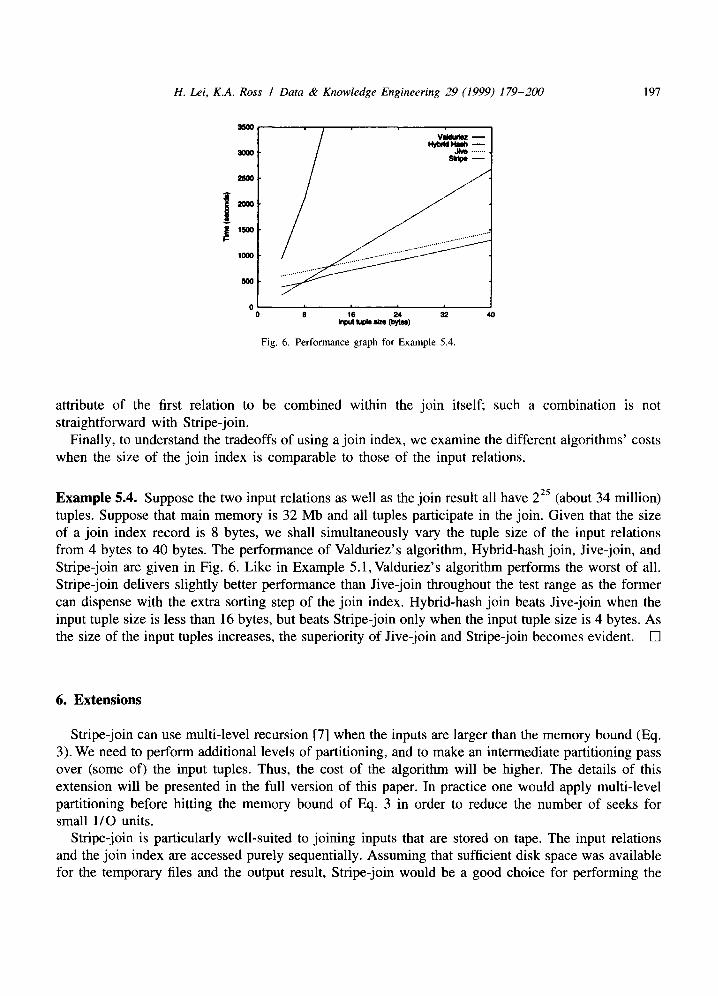
Fig. 6. Performance graph for Example 5.4.
attribute of the first relation to be combined within the join itself; such a combination is not straightforward with Stripe-join.
Finally, to understand the tradeoffs of using a join index, we examine the different algorithms' costs when the size of the join index is comparable to those of the input relations.
Example 5.4. Suppose the two input relations as well as the join result all have 225 (about 34 million) tuples. Suppose that main memory is 32 Mb and all tuples participate in the join. Given that the size of a join index record is 8 bytes, we shall simultaneously vary the tuple size of the input relations from 4 bytes to 40 bytes. The performance of Valduriez's algorithm, Hybrid-hash join, Jive-join, and Stripe-join are given in Fig. 6. Like in Example 5.1, Valduriez's algorithm performs the worst of all. Stripe-join delivers slightly better performance than Jive-join throughout the test range as the former can dispense with the extra sorting step of the join index. Hybrid-hash join beats Jive-join when the input tuple size is less than 16 bytes, but beats Stripe-join only when the input tuple size is 4 bytes. As the size of the input tuples increases, the superiority of Jive-join and Stripe-join becomes evident. []
6. Extensions
Stripe-join can use multi-level recursion [7] when the inputs are larger than the memory bound (Eq. 3). We need to perform additional levels of partitioning, and to make an intermediate partitioning pass over (some of) the input tuples. Thus, the cost of the algorithm will be higher. The details of this extension will be presented in the full version of this paper. In practice one would apply multi-level partitioning before hitting the memory bound of Eq. 3 in order to reduce the number of seeks for small I /O units.
Stripe-join is particularly well-suited to joining inputs that are stored on tape. The input relations and the join index are accessed purely sequentially. Assuming that sufficient disk space was available for the temporary files and the output result, Stripe-join would be a good choice for performing the

198 H. Lei, K.A. Ross / Data & Knowledge Engineering 29 (1999) 179-200
join with a pre-existing join index. Our cost model would have to be modified to model the characteristics of a tape drive.
There is a lot of potential parallelism in Stripe. Each of the input relations (and each of the segments within each relation) can, in principle, be processed independently. Compared with Jive-join, the parallelism in Stripe-join is more transparent since all relations are treated symmetrical- ly. In Jive-join there are two distinct phases: one relation must be completely processed before the other relations can be processed.
7. Conclusions
We have proposed a new algorithm, Stripe-join, for performing a join using a join index. 8 Like its predecessor Jive-join from [14,13], Stripe-join has the following properties: Almost all of the I /O performed is sequential. A block of an input relation is read if and only if it contains a record that participates in the join. Skew does not adversely affect the performance. One can join multiple relations, retaining the single-pass property of the inputs, by using multidimensional data structures. For a wide variety of examples, the algorithm outperforms conventional algorithms including Valduriez's algorithm and Hybrid-hash join.
Stripe-join has important advantages over Jive-join: • Jive-join requires a fixed ordering of the join index, while Stripe-join does not. Thus, Stripe-join
can avoid a sorting step. • For joins in which a relation R appears more than once, Stripe-join can make a single pass
through R to cover all of the instances of R in the join. In particular, self-joins can be performed with just one pass through the self-joined relation.
• Stripe-join delivers better performance under some circumstances, in particular when the cardinality of the join index is high.
To our knowledge Stripe-join is the first algorithm that, given a join index and a relation significantly larger than main memory, can perform a self-join with just a single passover the input relation and without storing input tuples in intermediate files.
Appendix A: The cost of jive-join
For completeness, we present the Jive-join costs formulas from [14,13]. Let z' denote ( r - 1)lJl/r. The corresponding formulas for the performance of Jive-join given in [14,13] a r e 9"
Ns = <lJI + IR, I + - ' - + Igrl + IJI/r) + (r - 2)y' + z ' / v + n I / x .
g , , o = Y(r, llglll, Ie,I/t , I Ie , l l )+"" + Y(rAIgrll, Ierl/t , IIRAt)÷ z ' / o ' + n, /x + 2 ( r - 1)y' + ]JI/fl + .
gx = I11 + 2z' + t Y( lle,ll, Iell/ , IJg,ll) + " " + t Y( llR, II, Ie,I/t , IIRill)- n 1 denotes II/ll*<<e, >>/b and the optimal values of x, y ' and v ' turn out to be:
We were informed by one of the referees that similar partitioning ideas have been used in the computation of Boolean functions by computing schemata [20].
9 There is a small change in the value of N s from [14,13]. Our estimate of N s is slightly more accurate because it allows for only one dimension whose partition order corresponds to the join result order.

H. Lei, K.A. Ross / Data & Knowledge Engineering 29 (1999) 179-200 199
m r m r L )
(x, v ' , y ' ) = L(1 + (r - 1 ) ~ ' L((r - 1) +X//-~/z) ' m r- '
where L = (IJl/r + 21R21)""" (IJl/r + 7-rlRrl).
A. 1. Sorting the Join index
When the join index is not clustered on one of its TID fields, we will have to sort the join index before Jive-join, Slam-join or Valduriez's algorithm can apply. We analyze the I /O cost for sorting a join index J. Since the I /O is mostly sequential, we shall ignore the seek and rotational latencies and just count the number of block transfers.
The sorting algorithm we use is a merge sort. We generate runs of length equal to the size of main memory, then merge those runs. (It is actually possible to generate runs that are twice as long as main memory [12], but the difference is immaterial in the present context.) The number of runs that are written to disk is FIJI/mT. On a single merge pass we can collapse n runs into Fn/m7 runs. The total number of block transfers during sorting is then 2(1 + FlogmF]J [/m77)lJI. (We can actually save up to 2m blocks by keeping the last run in memory, but the difference is not significant here.) This number needs to be added to the N x value for any algorithm that requires a sorted join index.
R e f e r e n c e s
[1] D.S. Batory, On searching transposed files, ACM Trans. on Database Systems 4(4) (1979) 531-544. [2] J. Blakeley, Nancy Martin, Join index, materialized view, and hybrid-hash join: A performance analysis. In: Proc. IEEE
Intl. Conf. on Data Eng. (1990) pp. 256-263. [3] M. Blasgen, K. Eswaran, Storage and access in relational data bases, IBM Systems Journal 16(4) (1977). [4] B. Bratbergsengen, Hashing methods and relational algebra operations. In: Proc. VLDB Conf. (August 1984) pp.
323-333. [5] K. Brown et al., Resource allocation and scheduling for mixed database workloads, Technical Report 1095, University
of Wisconsin, Madison (1992). [6] D.J. DeWitt et al., Implementation techniques for main memory database systems. In: Proc. ACM SIGMOD Conf. (June
1984) pp. 1-8. [7] G. Graefe, Performance enhancements for hybrid hash join. Technical Report 606, University of Colorado, Boulder
(1992). [8] L.M. Haas, M.J. Carey, M. Livny, Seeking the truth about ad hoc join costs, Technical Report RJ9368, IBM Almaden
Research Center (1993). [9] Laura M. Haas, Michael J. Carey, Miron Livny, Amit Shukla, Seeking the truth about ad hoc join costs, VLDB Journal
6(3) (1997) 241-256. [10] W. Kim, A new way to compute the product and join of relations. In: Proc. ACM SIGMOD Conf. (May 1980) pp.
179-187. [11] M. Kitsuregawa et al., Application of hash to data base machine and its architecture, New Generation Computing 1
(1983) 62-74. [ 12] Donald Ervin Knuth, Sorting and searching, Vol. 3, The Art of Computer Programming, Addison-Wesley, Reading, MA
(1973). [13] Z. Li, K. Ross, Fast joins using join indices, Technical Report CUCS-032-96, Columbia University (1996). [14] Z. Li, K. Ross, Fast joins using join indices, VLDB Journal (in press). [15] P. Mishra, M. Eich, Join processing in relational databases, ACM Computing Surveys 24(1) (March 1992).

200 H. Lei, K.A. Ross / Data &" Knowledge Engineering 29 (1999) 179-200
[16] C. Mohan, D. Haderle, Y. Wang, J. Cheng, Single table access using multiple indexes: Optimization, execution and concurrency control techniques. In: Proc. Int. Conf. on Extending Data Base Technology (1990).
[17] P. O'Neill, G. Graefe, Multi-table joins through bitmapped join indices, SIGMOD Record 24(3) (1995). [18] L. Shapiro, Join processing in database systems with large main memories, ACM Trans. on Database Systems 11(3)
(1986). [19] P. Valduriez, Join indices, ACM Trans. on Database Systems 12(2) (1987) 218-246. [20] Ingo Wegener, The Complexity of Boolean Functions Teubener-Wiley, Stuttgart (1987). [21] S.B. Yao, Approximating block accesses in database organizations, Comm. of the ACM 20(4) (1977) 260-261.
ltui Lei is a Research Staff Member at the IBM T.J. Watson Research center. His research interests include database systems, file systems, and distributed systems. He received a B.S. from Zongshan University, China in 1987, an M.S. from Courant Institute, New York University in 1989, and a Ph.D. from Columbia University in 1998, all in Computer Science. Prior to his doctoral career at Columbia, he was a Senior Software Engineer at Syncsort Inc.
Kenneth Ross is an Associate Professor of Computer Science at Columbia University. His research interests include database systems, data warehousing, query processing and optimization, and database theory. He is the recipient of an NSF Young Investigator Award, a Sloan Foundation Fellowship, and a Packard Foundation Fellowship. He received a B.Sc. (Hons.) from the University of Melbourne in 1986, and a Ph.D. from Stanford University in 1991.