fast volume rendering using a shear-warp factorization … · fast volume rendering using a...

COMPUTER GRAPHICS Proceedings, Annual Conference Series, 1994

9 4

Fast Volume Rendering Using a Shear-Warp Factorization of the Viewing Transformation

Philippe Lacroute

Computer Systems Laboratory Stanford University

Marc Levoy

Computer Science Department Stanford University

/"

Abstract

Several existing volume rendering algorithms operate by factor- ing the viewing transformation into a 3D shear parallel to the data slices, a projection to form an intermediate but distorted image, and a 2D warp to form an undistorted final image. We extend this class of algorithms in three ways. First, we describe a new object-order rendering algorithm based on the factorization that is significantly faster than published algorithms with minimal loss of image quality. Shear-warp factorizations have the property that rows of voxels in the volume are aligned with rows of pixels in the intermediate image. We use this fact to construct a scanline-based algorithm that traverses the volume and the intermediate image in synchrony, taking advantage of the spatial coherence present in both. We use spatial data structures based on run-length encoding for both the volume and the intermediate image. Our implementation running on an SGI Indigo workstation renders a 2563 voxel medical data set in one second. Our second extension is a shear- warp factorization for perspective viewing transformations, and we show how our rendering algorithm can support this extension. Third, we introduce a data structure for encoding spatial coherence in unclassified volumes (i.e. scalar fields with no precomputed opacity). When combined with our shear-warp rendering algorithm this data structure allows us to classify and render a 2563 voxel volume in three seconds. The method extends to support mixed volumes and geometry and is parallelizable.

CR Categories: 1.3.7 [Computer Graphics]: Three-Dimensional Graphics and Realism; 1.3.3 [Computer Graphics]: Picture/Image Generation--Display Algorithms.

Additional Keywords: Volume rendering, Coherence, Scientific visualization, Medical imaging.

1 Introduction

Volume rendering is a flexible technique for visualizing scalar fields with widespread applicability in medical imaging and scientific visualization, but its use has been limited because it is

Authors' Address: Center for Integrated Systems, Stanford University, Stanford, CA 94305-4070

E-mail: [email protected], [email protected] Word Wide Web: http://www-graphics.stanford.edu/

Permission to copy without fee all or part of this material is granted provided that the copies are not made or distributed for direct commercial advantage, the ACM copyright notice and the title of the publication and its date appear, and notice is given that copying is by permission of the Association for Computing Machinery. To copy otherwise, or to republish, requires a fee and/or specific permission.

computationally expensive. Interactive rendering rates have been reported using large parallel processors [17] [19] and using algorithms that trade off image quality for speed [10] [8], but high- quality images take tens of seconds or minutes to generate on current workstations. In this paper we present a new algorithm which achieves near-interactive rendering rates on a workstation without significantly sacrificing quality.

Many researchers have proposed methods that reduce rendering cost without affecting image quality by exploiting coherence in the data set. These methods rely on spatial data structures that encode the presence or absence of high-opacity voxels so that computation can be omitted in transparent regions of the volume. These data structures are built during a preprocessing step from a classified volume: a volume to which an opacity transfer function has been applied. Such spatial data structures include octrees and pyramids [13] [12] [8] [3], k-d trees [18] and distance transforms [23]. Although this type of optimization is data-dependent, researchers have reported that in typical classified volumes 70-95% of the voxels are transparent [12] [18].

Algorithms that use spatial data structures can be divided into two categories according to the order in which the data structures are traversed: image-order or object-order. Image-order algorithms operate by casting rays from each image pixel and processing the voxels along each ray [9]. This processing order has the disadvantage that the spatial data structure must be traversed once for every ray, resulting in redundant computation (e.g. multiple descents of an octree). In contrast, object-order algorithms operate by splatting voxels into the image while streaming through the volume data in storage order [20] [8]. However, this processing order makes it difficult to implement early ray termination, an effective optimization in ray-casting algorithms [12].

In this paper we describe a new algorithm which combines the advantages of image-order and object-order algorithms. The method is based on a factorization of the viewing matrix into a 3D shear parallel to the slices of the volume data, a projection to form a distorted intermediate image, and a 2D warp to produce the final image. Shear-warp factorizations are not new. They have been used to simplify data communication patterns in volume rendering algorithms for SIMD parallel processors [1] [17] and to simplify the generation of paths through a volume in a serial image-order algorithm [22]. The advantage of shear-warp factorizations is that scanlines of tlae volume data and scanlines of the intermediate image are always aligned. In previous efforts this property has been used to develop SIMD volume rendering algorithms. We exploit the property for a different reason: it allows efficient, synchro- nized access to data structures that separately encode coherence in the volume and the image.

The factorization also makes efficient, high-quality resampling possible in an object-order algorithm. In our algorithm the re-

© 1994 ACM-0-89791-667-0/94/007/0451 $01,50 451

SIGGRAPH 94, Orlando,Florida, July 24-29, 1994

viewing rays shear

volume slices roject

ima plane

varp

Figure 1: A volume is transformed to sheared object space for a parallel projection by translating each slice. The projection in sheared object space is simple and efficient.

viewing rays

)lume ices

shear and scale ~t

~roject

warp

ir lter of

P projection

Figure 2: A volume is transformed to sheared object space for a perspective projection by translating and scaling each slice. The projection in sheared object space is again simple and efficient.

sampling filter footprint is not view dependent, so the resampling complications of splatting algorithms [20] are avoided. Several other algorithms also use multipass resampling [4] [7] [19], but these methods require three or more resampling steps. Our algorithm requires only two resampling steps for an arbitrary perspective viewing transformation, and the second resampling is an inexpensive 2D warp. The 3D volume is traversed only once.

Our implementation running on an SGI Indigo workstation can render a 2563 voxel medical data set in one second, a factor of at least five faster than previous algorithms running on comparable hardware. Other than a slight loss due to the two-pass resampling, our algorithm does not trade off quality for speed. This is in contrast to algorithms that subsample the data set and can therefore miss small features [10] [3].

Section 2 of this paper describes the shear-warp factorization and its important mathematical properties. We also describe a new extension of the factorization for perspective projections. Section 3 describes three variants of our volume rendering algorithm. The first algorithm renders classified volumes with a parallel projection using our new coherence optimizations. The second algorithm supports perspective projections. The third algorithm is a fast classification algorithm for rendering unclassified volumes. Previous algorithms that employ spatial data structures require an expensive preprocessing step when the opacity transfer function changes. Our third algorithm uses a classification-independent rain-max octree data structure to avoid this step. Section 4 contains our performance results and a discussion of image quality. Finally we conclude and discuss some extensions to the algorithm in Section 5.

2 The Shear-Warp Factorization The arbitrary nature of the transformation from object space to image space complicates efficient, high-quality filtering and projection in object-order volume rendering algorithms. This problem can be solved by transforming the volume to an intermediate coordinate system for which there is a very simple mapping from the object coordinate system and which allows efficient projection.

We call the intermediate coordinate system "sheared object space" and define it as follows:

Definition 1: By construction, in sheared object space all viewing rays are parallel to the third coordinate axis.

Figure 1 illustrates the transformation from object space to sheared object space for a parallel projection. We assume the volume is sampled on a rectilinear grid. The horizontal lines in the figure represent slices of the volume data viewed in cross-section. After transformation the volume data has been sheared parallel to the set of slices that is most perpendicular to the viewing direction and

the viewing rays are perpendicular to the slices. For a perspective transformation the definition implies that each slice must be scaled as well as sheared as shown schematically in Figure 2.

Definition 1 can be formalized as a set of equations that transform object coordinates into sheared object coordinates. These equations can be written as a factorization of the view transfor- marion matrix Mview as follows:

Mview = P ' S - Mwaw

P is a permutation matrix which transposes the coordinate system in order to make the z-axis the principal viewing axis. S transforms the volume into sheared object space, and M w ~ transforms sheared object coordinates into image coordinates. Cameron and Undrill [1] and SchrSder and Stoll [17] describe this factorization for the case of rotation matrices. For a general parallel projection S has the form of a shear perpendicular to the z-axis: (1000)

Spar = 0 1 0 0 Sx sv 1 0 0 0 0 1

where s= and s u can be computed from the elements of Mview. For perspective projections the transformation to sheared object space is of the form:

1 0 0 0 / Sper~p 0 1 0 0

- ~ l i 1 i '-qx 8y s w 0 0 0 1

This matrix specifies that to transform a particular slice z0 of voxel data from object space to sheared object space the slice must be translated by (zos~, zos~) and then scaled uniformly by 1/(1 + z0s~). The final term of the factorization is a matrix which warps sheared object space into image space:

Mwarp = S-1 . p - 1 . Mview

A simple volume rendering algorithm based on the shear-warp factorization operates as follows (see Figure 3):

1. Transform the volume data to sheared object space by translating and resampling each slice according to S. For perspective transformations, also scale each slice. P specifies which of the three possible slicing directions to use.

2. Composite the resampled slices together in front-to-back order using the "over" operator [15]. This step projects the volume into a 2D intermediate image in sheared object space.

452


1. shear & ~ resample/ r4.... ~

L / intermediate voxel l~~l lJ¢~ql[ / imagescanl ine scanline ~ ~""""',,,,,,,,,,,,~....~ I 3. warp &

voxel slice intermediate image final image

Figure 3: The shear-warp algorithm includes three conceptual steps: shear and resample the volume slices, project resampled voxel scanlines onto intermediate image scanlines, and warp the intermediate image into the final image.

3. Transform the intermediate image to image space by warping it according to Mw~. This second resampling step produces the correct final image.

The parallel-projection version of this algorithm was first described by Cameron and Undrill [l]. Our new optimizations are described in the next section.

The projection in sheared object space has several geometric properties that simplify the compositing step of the algorithm:

Property 1: Scanlines of pixels in the intermediate image are parallel to scanlines of voxels in the volume data.

Property 2: All voxels in a given voxel slice are scaled by the same factor.

Property 3 (parallel projections only): Every voxel slice has the same scale factor, and this factor can be chosen arbitrarily. In particular, we can choose a unity scale factor so that for a given voxel scanline there is a one-to-one mapping between voxels and intermediate-image pixels.

In the next section we make use of these properties.

3 Shear-Warp Algorithms We have developed three volume rendering algorithms based on the shear-warp factorization. The first algorithm is optimized for parallel projections and assumes that the opacity transfer function does not change between renderings, but the viewing and shading parameters can be modified. The second algorithm supports perspective projections. The third algorithm allows the opacity transfer function to be modified as well as the viewing and shading parameters, with a moderate performance penalty.

3.1 Parallel Projection Rendering Algorithm Property 1 of the previous section states that voxel scanlines in the sheared volume are aligned with pixel scanlines in the intermediate image, which means that the volume and image data structures can

I I opaque pixel

D non-opaque pixel

Figure 4: Offsets stored with opaque pixels in the intermediate image allow occluded voxels to be skipped efficiently.

both be traversed in scanline order. Scanline-based coherence data structures are therefore a natural choice. The first data structure we use is a run-length encoding of the voxel scanlines which allows us to take advantage of coherence in the volume by skipping runs of transparent voxels. The encoded scanlines consist of two types of runs, transparent and non-transparent, defined by a user-specified opacity threshold. Next, to take advantage of coherence in the image, we store with each opaque intermediate image pixel an offset to the next non-opaque pixel in the same scanline (Figure 4). An image pixel is defined to be opaque when its opacity exceeds a user-specified threshold, in which case the corresponding voxels in yet-to-be-processed slices are occluded. The offsets associated with the image pixels are used to skip runs of opaque pixels without examining every pixel. The pixel array and the offsets form a run-length encoding of the intermediate image which is computed on-the-fly during rendering.

These two data structures and Property 1 lead to a fast scanline- based rendering algorithm (Figure 5). By marching through the volume and the image simultaneously in scanline order we reduce addressing arithmetic. By using the run-length encoding of the voxel data to skip voxels which are transparent and the run-length encoding of the image to skip voxels which are occluded, we per- form work only for voxels which are both non-transparent and visible.

For voxel runs that are not skipped we use a tightly-coded loop that performs shading, resampling and compositing. Prop- erties 2 and 3 allow us to simplify the resampling step in this loop. Since the transformation applied to each slice of volume data before projection consists only of a translation (no scaling or rotation), the resampling weights are the same for every voxel in a slice (Figure 6). Algorithms which do not use the shear-warp factorization must recompute new weights for every voxel. We use a bilinear interpolation filter and a gather-type convolution (backward projection): two voxel scanlines are traversed simultaneously to compute a single intermediate image scanline at a time. Scatter-type convolution (forward projection) is also possible. We use a lookup-table based system for shading [6]. We also use a lookup table to correct voxel opacity for the current viewing angle

voxel scanline: ! [ ] [ I I

" | resample and '

I ' composite image !ntermediate : i ! :

scanline: ~ ~! ~! =! ~ : =.. skip i work ! skip i work I skip

[ ] transparent voxel run • opaque image pixel run

[ ] non-transparent voxel run [ ] non-opaque image pixel run

Figure 5: Resampling and compositing are performed by streaming through both the voxels and the intermediate image in scanline order, skipping over voxels which are transparent and pixels which are opaque.

453

SlGGRAPH 94, Orlando, Florida, July 24-29, 1994

• original voxel

© resampled voxel

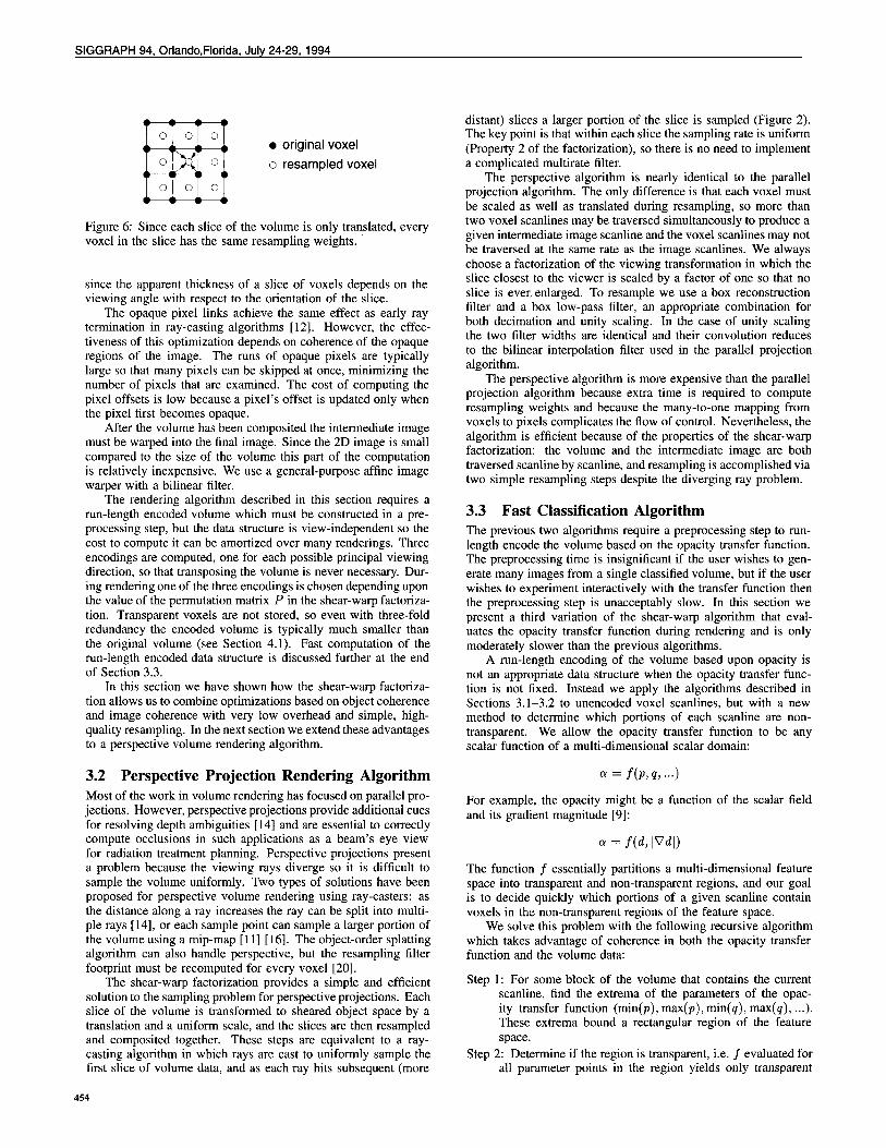
Figure 6: Since each slice of the volume is only translated, every voxel in the slice has the same resampling weights.

since the apparent thickness of a slice of voxels depends on the viewing angle with respect to the orientation of the slice.

The opaque pixel links achieve the same effect as early ray termination in ray-casting algorithms [12]. However, the effectiveness of this optimization depends on coherence of the opaque regions of the image. The runs of opaque pixels are typically large so that many pixels can be skipped at once, minimizing the number of pixels that are examined. The cost of computing the pixel offsets is low because a pixel's offset is updated only when the pixel first becomes opaque.

After the volume has been composited the intermediate image must be warped into the final image. Since the 2D image is small compared to the size of the volume this part of the computation is relatively inexpensive. We use a general-purpose affine image warper with a bilinear filter.

The rendering algorithm described in this section requires a run-length encoded volume which must be constructed in a preprocessing step, but the data structure is view-independent so the cost to compute it can be amortized over many renderings. Three encodings are computed, one for each possible principal viewing direction, so that transposing the volume is never necessary. Dur- ing rendering one of the three encodings is chosen depending upon the value of the permutation matrix P in the shear-warp factorization. Transparent voxels are not stored, so even with three-fold redundancy the encoded volume is typically much smaller than the original volume (see Section 4.1). Fast computation of the run-length encoded data structure is discussed further at the end of Section 3.3.

In this section we have shown how the shear-warp factorization allows us to combine optimizations based on object coherence and image coherence with very low overhead and simple, high- quality resampling. In the next section we extend these advantages to a perspective volume rendering algorithm.

3.2 Perspective Projection Rendering Algorithm Most of the work in volume rendering has focused on parallel projections. However, perspective projections provide additional cues for resolving depth ambiguities [14] and are essential to correctly compute occlusions in such applications as a beam's eye view for radiation treatment planning. Perspective projections present a problem because the viewing rays diverge so it is difficult to sample the volume uniformly. Two types of solutions have been proposed for perspective volume rendering using ray-casters: as the distance along a ray increases the ray can be split into multiple rays [14], or each sample point can sample a larger portion of the volume using a mip-map [11] [16]. The object-order splatting algorithm can also handle perspective, but the resampling filter footprint must be recomputed for every voxel [20].

The shear-warp factorization provides a simple and efficient solution to the sampling problem for perspective projections. Each slice of the volume is transformed to sheared object space by a translation and a uniform scale, and the slices are then resampled and composited together. These steps are equivalent to a ray- casting algorithm in which rays are cast to uniformly sample the first slice of volume data, and as each ray hits subsequent (more

distant) slices a larger portion of the slice is sampled (Figure 2). The key point is that within each slice the sampling rate is uniform (Property 2 of the factofization), so there is no need to implement a complicated multirate filter.

The perspective algorithm is nearly identical to the parallel projection algorithm. The only difference is that each voxel must be scaled as well as translated during resampling, so more than two voxel scanlines may be traversed simultaneously to produce a given intermediate image scanline and the voxel scanlines may not be traversed at the same rate as the image scanlines. We always choose a factorization of the viewing transformation in which the slice closest to the viewer is scaled by a factor of one so that no slice is ever! enlarged. To resample we use a box reconstruction filter and a box low-pass filter, an appropriate combination for both decimation and unity scaling. In the case of unity scaling the two filter widths are identical and their convolution reduces to the bilinear interpolation filter used in the parallel projection algorithm.

The perspective algorithm is more expensive than the parallel projection algorithm because extra time is required to compute resampling weights and because the many-to-one mapping from voxels to pixels complicates the flow of control. Nevertheless, the algorithm is efficient because of the properties of the shear-warp factorization: the volume and the intermediate image are both traversed scanline by scanline, and resampling is accomplished via two simple resampling steps despite the diverging ray problem.

3.3 Fast Classification Algorithm The previous two algorithms require a preprocessing step to run- length encode the volume based on the opacity transfer function. The preprocessing time is insignificant if the user wishes to generate many images from a single classified volume, but if the user wishes to experiment interactively with the transfer function then the preprocessing step is unacceptably slow. In this section we present a third variation of the shear-warp algorithm that eval- uates the opacity transfer function during rendering and is only moderately slower than the previous algorithms.

A run-length encoding of the volume based upon opacity is not an appropriate data structure when the opacity transfer function is not fixed. Instead we apply the algorithms described in Sections 3.1-3.2 to unencoded voxel scanlines, but with a new method to determine which portions of each scanline are non- transparent. We allow the opacity transfer function to be any scalar function of a multi-dimensional scalar domain:

= f(p, q .... )

For example, the opacity might be a function of the scalar field and its gradient magnitude [9]:

o~ = f ( d , 1~7dl)

The function f essentially partitions a multi-dimensional feature space into transparent and non-transparent regions, and our goal is to decide quickly which portions of a given scanline contain voxels in the non-transparent regions of the feature space.

We solve this problem with the following recursive algorithm which takes advantage of coherence in both the opacity transfer function and the volume data:

Step 1: For some block of the volume that contains the current scanline, find the extrema of the parameters of the opacity transfer function (min(p),max(p),min(q), max(q) .... ). These extrema bound a rectangular region of the feature space.

Step 2: Determine if the region is transparent, i.e. f evaluated for all parameter points in the region yields only transparent

454


~ summed area table

--~ R - - ~ f ( p , q )

min-max octree Pmin Pma~- (a) (b) (c)

9 - 0

Figure 7: A min-max octree (a) is used to determine the range of the parameters p, q of the opacity transfer function f(p, q) in a subcube of the volume. A summed area table (b) is used to integrate f over that range of p, q. If the integral is zero (c) then the subcube contains only transparent voxels.

opacities. If so, then discard the scanline since it must be transparent.

Step 3: Subdivide the scanline and repeat this algorithm recur- sively. If the size of the current scanline portion is below a threshold then render it instead of subdividing.

This algorithm relies on two data structures for efficiency (Fig- ure 7). First, Step 1 uses a precomputed min-max octree [21]. Each octree node contains the extrema of the parameter values for a subcube of the volume. Second, to implement Step 2 of the algorithm we need to integrate the function f over the region of the feature space found in Step 1. If the integral is zero then all voxels must be transparent.* This integration can be performed in constant time using a multi-dimensional summed-area table [2] [5]. The voxels themselves are stored in a third data structure, a simple 3D array.

The overall algorithm for rendering unclassified data sets pro- ceeds as follows. The rain-max octree is computed at the time the volume is first loaded since the octree is independent of the opacity transfer function and the viewing parameters. Next, just before rendering begins the opacity transfer function is used to compute the summed area table. This computation is inexpensive provided that the domain of the opacity transfer function is not too large. We then use either the parallel projection or the perspective projection rendering algorithm to render voxels from an unencoded 3D voxel array. The array is traversed scanline by scanline. For each scanline we use the octree and the summed area table to determine which portions of the scanline are non-transparent. Voxels in the non-transparent portions are individually classified using a lookup table and rendered as in the previous algorithms. Opaque regions of the image are skipped just as before. Note that voxels that are either transparent or occluded are never classified, which reduces the amount of computation.

The octree traversal and summed area table lookups add overhead to the algorithm which were not present in the previous algorithms. In order to reduce this overhead we save as much computed data as possible for later reuse: an octree node is tested for transparency using the summed area table only the first time it is visited and the result is saved for subsequent traversals, and if two adjacent scanlines intersect the same set of octree nodes then we record this fact and reuse information instead of making multiple traversals.

This rendering algorithm places two restrictions on the opacity transfer function: the parameters of the function must be precom- putable for each voxel so that the octree may be precomputed, and the total number of possible argument tuples to the function (the cardinality of the domain) must not be too large since the

*The user may choose a non-zero opacity threshold for transparent voxels, in which case a thresholded version of f must be integrated: let ] ' = f whenever f exceeds the threshold, and f J = 0 otherwise.

summed area table must contain one entry for each possible tu- pie. Context-sensitive segmentation (classification based upon the position and surroundings of a voxel) does not meet these criteria unless the segmentation is entirely precomputed.

The fast-classification algorithm presented here also suffers from a problem common to many object-order algorithms: if the major viewing axis changes then the volume data must be ac- cessed against the stride and performance degrades. Alternatively the 3D array of voxels can be transposed, resulting in a delay during interactive viewing. Unlike the algorithms based on a run- length encoded volume, it is typically not practical to maintain three copies of the unencoded volume since it is much larger than a run-length encoding. It is better to use a small range of view- points while modifying the classification function, and then to switch to one of the previous two rendering methods for rendering animation sequences. In fact, the octree and the summed-area table can be used to convert the 3D voxel array into a run-length encoded volume without accessing transparent voxels, leading to a significant time savings (see the "Switch Modes" arrow in Fig- ure 12). Thus the three algorithms fit together well to yield an interactive tool for classifying and viewing volumes.

4 Results

4.1 S p e e d a n d Memory Our performance results for the three algorithms are summarized in Table 1. The "Fast Classification" timings are for the algorithm in Section 3.3 with a parallel projection. The timings were mea- sured on an SGI Indigo R4000 without hardware graphics accel- erators. Rendering times include all steps required to render from a new viewpoint, including computation of the shading lookup table, compositing and wmping, hut the preprocessing step is not included. The "Avg." field in the table is the average time in seconds for rendering 360 frames at one degree angle increments, and the "Min/Max" times are for the best and worst case angles. The "Mem." field gives the size in megabytes of all data structures. For the first two algorithms the size includes the three run-length encodings of the volume, the image data structures and all lookup tables. For the third algorithm the size includes the unencoded volume, the octree, the summed-area table, the image data structures, and the lookup tables. The "brain" data set is an MRI scan of a human head (Figure 8) and the "head" data set is a CT scan of a human head (Figure 9). The "brainsmall" and "headsmall" data sets are decimated versions of the larger volumes.

The timings are nearly independent of image size because this factor affects only the final wa R which is relatively insignificant. Rendering time is dependent on viewing angle (Figure 11) because the effectiveness of the coherence optimizations varies with viewpoint and because the size of the intermediate image increases as the rotation angle approaches 45 degrees, so more compositing operations must be performed. For the algorithms described in Sections 3.1-3.2 there is no jump in rendering time when the major viewing axis changes, provided the three run-length encoded copies of the volume fit into real memory simultaneously. Each copy contains four bytes per non-transparent voxel and one byte per run. For the 256x256x226 voxel head data set the three run- length encodings total only 9.8 Mbytes. All of the images were rendered on a workstation with 64 Mbytes of memory. To test the fast classification algorithm (Section 3.3) on the 256 ~ data sets we used a workstation with 96 Mbytes of memory.

Figure 12 gives a breakdown of the time required to render the brain data set with a parallel projection using the fast classification algorithm (left branch) and the parallel projection algorithm (right branch). The time required to warp the intermediate image into the final image is typically 10-20% of the total rendering time for the parallel projection algorithm. The "Switch Modes" arrow

455

SIGGRAPH 94, Orlando, Florida, July 24-29, 1994

Data set

brainsmall headsmall brain head

Size (voxels)

128x128x109 128x128x113 256x256x167 256x256x225

Parallel projection (§ 3.1) Avg. Min/Max Mere. 0.4 s. 0.37-0.48 s. 4 Mb. 0.4 0.35-0.43 2 1.1 0.91-1.39 19 1.2 1.04-1.33 13

Perspective projection (§3.2) Fast classification (§3.3) Avg. Min/Max Mem. Avg. Min/Max Mem. 1.0 s. 0.84-1.13 s. 4 Mb. 0.7 s. 0.61-0.84 s. 8 Mb. 0.9 0.82-1.00 2 0.8 0.72-0.87 8 3.0 2.44-2.98 19 2.4 1.91-2.91 46 3.3 2.99-3.68 13 2.8 2.43-3.23 61

Table 1: Rendering time and memory usage on an SGI Indigo workstation. Times are in seconds and include shading, resampling, projection and warping. The fast classification times include rendering with a parallel projection. The "Mem." field is the total size of the data structures used by each algorithm.

1500 - d

"~'1000 I- ~g

" E

~- 500 - E

Max: 1330 msec. Min: 1039 msec. Avg: 1166 msec.

0 I I I I 0 90 180 270 360

Rotation Angle (Degrees)

Figure 11 : Rendering time for a parallel projection of the head data set as the viewing angle changes.

shows the time required for all three copies of the run-length encoded volume to be computed from the unencoded volume and the min-max octree once the user has settled on an opacity transfer function.

The timings above are for grayscale renderings. Color renderings take roughly twice as long for parallel projections and 1.3x longer for perspective because of the additional resampling required for the two extra color channels. Figure 13 is a color rendering of the head data set classified with semitransparent skin which took 3.0 sec. to render. Figure 14 is a rendering of a 256x256x 110 voxel engine block, classified with semi-transparent and opaque surfaces; it took 2.3 sec. to render. Figure 15 is a rendering of a 256x256x159 CT scan of a human abdomen, rendered in 2.2 sec. The blood vessels of the subject contain a radio-opaque dye, and the data set was classified to reveal both the dye and bone surfaces. Figure 16 is a perspective color rendering of the engine data set which took 3.8 sec. to compute.

For comparison purposes we rendered the head data set with a ray-caster that uses early ray termination and a pyramid to exploit object coherence [12]. Because of its lower computational overhead the shear-warp algorithm is more than five times faster for the 1283 data sets and more than ten times faster for the 2563 data sets. Our algorithm running on a workstation is competitive with algorithms for massively parallel processors ([17], [19] and others), although the parallel implementations do not rely on coherence optimizations and therefore their performance results are not data dependent as ours are.

Our experiments show that the running time of the algorithms in Sections 3.1-3.2 is proportional to the number of voxels which are resampled and composited. This number is small either if a significant fraction of the voxels are transparent or if the average voxel opacity is high. In the latter case the image quickly becomes opaque and the remaining voxels are skipped. For the data sets and classification functions we have tried roughly n 2 voxels are both non-transparent and visible, so we observe O(n 2) performance as shown in Table 1: an eight-fold increase in the

~ P r e p r o c e s s Dataset

. . . . . . . . t 77sec.____ Switc

I v°lume + l octree • 2280 msec.

intermediateimage I . ~ 0 msec.

New Classification- i~:3-.:3)

Switch Modes

8.5 sec. ,I run-length I encoding I

980 msec.

intermediateimage I

e l 0 msec. ;

New viewpoint (§3.1)

Figure 12: Performance results for each stage of rendering the brain data set with a parallel projection. The left side uses the fast classification algorithm and the right side uses the parallel projection algorithm.

number of voxels leads to only a four-fold increase in time for the compositing stage and just under a four-fold increase in overall rendering time. For our rendering of the head data set 5% of the voxels are non-transparent, and for the brain data set 11% of the voxels are non-transparent. Degraded performance can be ex- pected if a substantial fraction of the classified volume has low but non-transparent opacity, but in our experience such classification functions are less useful.

4.2 Image Quality Figure 10 is a volume rendering of the same data set as in Figure 9, but produced by a ray-caster using tfilinear interpolation [12]. The two images are virtually identical.

Nevertheless, there are two potential quality problems associated with the shear-warp algorithm. First, the algorithm involves two resampling steps: each slice is resampled during compositing, and the intermediate image is resampled during the final warp. Multiple resampling steps can potentially cause blurring and loss of detail. However even in the high-detail regions of Figure 9 this effect is not noticeable.

The second potential problem is that the shear-warp algorithm uses a 2D rather than a 3D reconstruction filter to resample the volume data. The bilinear filter used for resampling is a first-order filter in the plane of a voxel slice, but it is a zero-order (nearest- neighbor) filter in the direction orthogonal to the slice. Artifacts are likely to appear if the opacity or color attributes of the volume contain very high frequencies (although if the frequencies exceed the Nyquist rate then perfect reconstruction is impossible).

456


Figure 17 shows a case where a trilinear interpolation filter outperforms a bilinear filter. The left-most image is a rendering by the shear-warp algorithm of a portion of the engine data set which has been classified with extremely sharp ramps to produce high frequencies in the volume's opacity. The viewing angle is set to 45 degrees relative to the slices of the data set--the worst case--and aliasing is apparent. For comparison, the middle image is a rendering produced with a ray-caster using trilinear interpolation and otherwise identical rendering parameters; here there is virtually no aliasing. However, by using a smoother opacity transfer function these reconstruction artifacts can be reduced. The fight-most image is a rendering using the shear-warp algorithm and a less-extreme opacity transfer function. Here the aliasing is barely noticeable because the high frequencies in the scalar field have effectively been low-pass filtered by the transfer function. In practice, as long as the opacity transfer function is not a binary classification the bilinear filter produces good results.

5 Conclusion

The shear-warp factorization allows us to implement coherence optimizations for both the volume data and the image with low computational overhead because both data structures can be traversed simultaneously in scanline order. The algorithm is flexible enough to accommodate a wide range of user-defined shading models and can handle perspective projections. We have also presented a variant of the algorithm that does not assume a fixed opacity transfer function. The result is an algorithm which produces high-quality renderings of a 2563 volume in roughly one second on a workstation with no specialized hardware.

We are currently extending our rendering algorithm to support data sets containing both geometry and volume data. We have also found that the shear-warp algorithms parallelize naturally for MIMD shared-memory multiprocessors. We parallelized the resampling and compositing steps by distributing scanlines of the intermediate image to the processors. On a 16 processor SGI Challenge multiprocessor the 256x256x223 voxel head data set can be rendered at a sustained rate of 10 frames/sec.

Acknowledgements

We thank Pat Hanrahan, Sandy Napel and North Carolina Memo- rial Hospital for the data sets, and Maneesh Agrawala, Mark Horowitz, Jason Nieh, Dave Ofelt, and Jaswinder Pal Singh for their help. This research was supported by Software Publish- ing Corporation, ARPA/ONR under contract N00039-91-C-0138, NSF under contract CCR-9157767 and the sponsoring companies of the Stanford Center for Integrated Systems.

References

[1] Cameron, G. G. and P. E. Undrill. Rendering volumetric medical image data on a SIMD-architecture computer. In Proceedings of the Third Eurographics Workshop on Ren- dering, 135-145, Bristol, UK, May 1992.

[2] Crow, Franklin C. Summed-area tables for texture mapping. Proceedings of SIGGRAPH '84. Computer Graphics, 18(3):207-212, July 1984.

[3] Danskin, John and Pat Hanrahan. Fast algorithms for volume ray tracing. In 1992 Workshop on Volume Visualization, 91- 98, Boston, MA, October 1992.

[4] Drebin, Robert A., Loren Carpenter and Pat Hanrahan. Vol- ume rendering. Proceedings of SIGGRAPH '88. Computer Graphics, 22(4):65-74, August 1988.

[5] Glassner, Andrew S. Multidimensional sum tables. In Graphics Gems, 376-381. Academic Press, New York, 1990.

[6] Glassner, Andrew S. Normal coding. In Graphics Gems, 257-264. Academic Press, New York, 1990.

[7] Hanrahan, Pat. Three-pass affine transforms for volume rendering. Computer Graphics, 24(5):71-77, November 1990.

[8] Laur, David and Pat Hanrahan. Hierarchical splatting: A progressive refinement algorithm for volume rendering. Proceedings of SIGGRAPH '91. Computer Graphics, 25(4):285-288, July 1991.

[9] Levoy, Marc. Display of surfaces from volume data. IEEE Computer Graphics & Applications, 8(3):29-37, May 1988.

[10] Levoy, Marc. Volume rendering by adaptive refinement. The Visual Computer, 6(1):2-7, February 1990.

[11] Levoy, Marc and Ross Whitaker. Gaze-directed volume rendering. Computer Graphics, 24(2):217-223, March 1990.

[12] Levoy, Marc. Efficient ray tracing of volume data. ACM Transactions on Graphics, 9(3):245-261, July 1990.

[13] Meagher, Donald J. Efficient synthetic image generation of arbitrary 3-D objects. In Proceeding of the IEEE Confer- ence on Pattern Recognition and Image Processing, 473- 478, 1982.

[14] Novins, Kevin L., Francois X. Sillion, and Donald P. Green- berg. An efficient method for volume rendering using perspective projection. Computer Graphics, 24(5):95-102, November 1990.

[15] Porter, Thomas and Tom Duff. Compositing digital images. Proceedings of SIGGRAPH '84. Computer Graphics, 18(3):253-259, July 1984.

[16] Sakas, Georgios and Matthias Gerth. Sampling and anti- aliasing of discrete 3-D volume density textures. In Proceed- ings of Eurographics '91, 87-102, Vienna, Austria, Septem- ber 1991.

[17] Schr~der, Peter and Gordon Stoll. Data parallel volume rendering as line drawing. In Proceedings of the 1992 Workshop on Volume Visualization, 25-32, Boston, October 1992.

[18] Subramanian, K. R. and Donald S. Fussell. Applying space subdivision techniques to volume rendering. In Proceedings of Visualization '90, 150-159, San Francisco, California, Oc- tober 1990.

[19] V6zina, Guy, Peter A. Fletcher, and Philip K. Robertson. Volume rendering on the MasPar MP-1. In 1992 Workshop on Volume Visualization, 3-8, Boston, October 1992.

[20] Westover, Lee. Footprint evaluation for volume rendering. Proceedings of SIGGRAPH '90. Computer Graphics, 24(4):367-376, August 1990.

[21] Wilhelms, Jane and Allen Van Gelder. Octrees for faster isosurface generation. Computer Graphics, 24(5):57-62, November 1990.

[22] Yagel, Roni and Arie Kaufman. Template-based volume viewing. In Eurographics 92, C-153-167, Cambridge, UK, September 1992.

[23] Zuiderveld, Karel J., Anton H.J. Koning, and Max A. Viergever. Acceleration of ray-casting using 3D distance transforms. In Proceedings of Visualization in Biomedical Computing 1992, 324-335, Chapel Hill, North Carolina, Oc- tober 1992.

457

SIGGRAPH 94, Orlando, Florida, July 24-29, 1994

Figure 8: Volume rendering with a parallel projection of an MRI scan of a human brain using the shear-warp algorithm (1.1 sec.).

Figure 9: Volume rendering with a parallel projection of a CT scan of a human head oriented at 45 degrees relative to the axes of the volume (1.2 sec.).

Figure 10: Volume rendering of the same data set as in Figure 9 using a ray-caster [12] for quality comparison (13.8 sec.).

Figure 13: Volume rendering with a parallel projection of the human head data set classified with semitransparent skin (3.0 sec.).

Figure 14: Volume rendering with a parallel projection of an engine block with semitransparent and opaque surfaces (2.3 sec.).

Figure 15: Volume rendering with a parallel projection of a CT scan of a human abdomen (2.2 sec.). The blood vessels contain a radio-opaque dye.

Figure 16: Volume rendering with a perspective projection of the engine data set (3.8 sec.).

(a) (b) (c)

Figure 17: Comparison of image quality with bilinear and trilinear filters for a portion of the engine data set. The images have been enlarged. (a) Bilinear filter with binary classification. (b) Trilinear filter with binary classification. (c) Bilinear filter with smooth classification.

458

fast volume rendering using a shear-warp factorization … · fast volume rendering using a...

Documents