econstorMake Your Publication Visible

A Service of

zbwLeibniz-InformationszentrumWirtschaftLeibniz Information Centrefor Economics

Bienz, Carsten; Thorburn, Karin; Walz, Uwe

Working Paper

Coinvestment and risk taking in private equity funds

SAFE Working Paper Series, No. 126

Provided in Cooperation with:Research Center SAFE - Sustainable Architecture for Finance in Europe,Goethe University Frankfurt

Suggested Citation: Bienz, Carsten; Thorburn, Karin; Walz, Uwe (2016) : Coinvestment and risktaking in private equity funds, SAFE Working Paper Series, No. 126

This Version is available at:http://hdl.handle.net/10419/129062

Standard-Nutzungsbedingungen:

Die Dokumente auf EconStor dürfen zu eigenen wissenschaftlichenZwecken und zum Privatgebrauch gespeichert und kopiert werden.

Sie dürfen die Dokumente nicht für öffentliche oder kommerzielleZwecke vervielfältigen, öffentlich ausstellen, öffentlich zugänglichmachen, vertreiben oder anderweitig nutzen.

Sofern die Verfasser die Dokumente unter Open-Content-Lizenzen(insbesondere CC-Lizenzen) zur Verfügung gestellt haben sollten,gelten abweichend von diesen Nutzungsbedingungen die in der dortgenannten Lizenz gewährten Nutzungsrechte.

Terms of use:

Documents in EconStor may be saved and copied for yourpersonal and scholarly purposes.

You are not to copy documents for public or commercialpurposes, to exhibit the documents publicly, to make thempublicly available on the internet, or to distribute or otherwiseuse the documents in public.

If the documents have been made available under an OpenContent Licence (especially Creative Commons Licences), youmay exercise further usage rights as specified in the indicatedlicence.

www.econstor.eu

Coinvestment and risk taking in private equity funds∗

Carsten Bienz

Norwegian School of Economics

Karin S. Thorburn

Norwegian School of Economics, CEPR and ECGI

Uwe Walz

Goethe University Frankfurt

January 2016

Abstract

Private equity fund managers are typically required to invest their own money alongside

the fund. We examine how this coinvestment affects the acquisition strategy of leveraged

buyout funds. In a simple model, where the investment and capital structure decisions

are made simultaneously, we show that a higher coinvestment induces managers to chose

less risky firms and use more leverage. We test these predictions in a unique sample of

private equity investments in Norway, where the fund manager’s taxable wealth is publicly

available. Consistent with the model, portfolio company risk decreases and leverage ratios

increase with the coinvestment fraction of the manager’s wealth. Moreover, funds requiring

a relatively high coinvestment tend to spread its capital over a larger number of portfolio

firms, consistent with a more conservative investment policy.

Keywords: Private equity, leveraged buyouts, incentives, coinvestment, risk taking, wealth

JEL Classification: D86, G12, G31, G32, G34.

∗We are grateful for comments by Ulf Axelson, Francesca Cornelli, Alexander Ljunqvist, Tiago Pinheiro,Morten Sorensen, Joacim Tag, Lucy White and seminar participants at BI, DBJ, Hitotusbashi, NHH, Nagoyaand the 8th Private Equity Findings Symposium at LBS. Parts of this paper were written when Carsten Bienzwas visiting Development Bank of Japan. We would also like to thank Marit Hofset Stamnes for research support.We gratefully acknowledge research support from the Research Center SAFE, funded by the State of Hesseninitiative for research LOEWE; Emails: carsten.bienz@nhh.no; karin.thorburn@nhh.no; and uwalz@econ.uni-frankfurt.de.

1 Introduction

Private equity funds are raised and managed by a general partner (GP), who makes the in-

vestment decisions for the fund. GPs are compensated with a mix of fixed and variable fees.

A typical compensation structure is a two percent annual management fee on the fund’s cap-

ital and a 20% carried interest on the profits above a certain threshold (Metrick and Yasuda,

2010). In addition, many GPs charge transaction fees and monitoring fees to their portfolio

companies (Phalippou, 2009).1

This fee structure creates an option-like payoff, with little downside to the managers of the

fund. Since the GP’s ability to raise future funds also depends on the current performance,

the incentives to generate high returns is even stronger than it may first appear (Chung et al.,

2012). Extant evidence suggests that corporate managers with large stock option holdings

tend to take more risk (Coles et al., 2006; Knopf et al., 2002; Shue and Townsend, 2013). If

the GP compensation structure encourages excessive risk taking, it could potentially have an

adverse effect on fund value.2

To counteract incentives to gamble with the fund’s money, managers are typically required

to coinvest their own money in the portfolio companies alongside the private equity fund. This

“skin in the game” forces the GP to participate in any losses incurred by the fund.3 A typical

GP in the US is required to invest 1% of the fund’s capital, corresponding to a $3.6 million

investment (Robinson and Sensoy, 2015).4 While a large coinvestment mitigates incentives

for excessive risk taking, it may also make a risk-averse manager too conservative, foregoing

valuable investment opportunities with high risk.

In this paper, we are the first to examine how the coinvestment affects the investment

decisions of private equity fund managers.

We start by developing a simple theoretical model, in which the selection of a target firm

and the decision on deal financing are made simultaneously. Fund managers can chose between

1Phalippou (2009) estimates the average annual fees to 7% of the private equity fund’s capital.2See, for example, Thanassoulis (2012), where large bonus payments triggered by competition for banker

talent increase the default risk.3Edmans and Liu (2011) argue that inside debt provides an efficient solution to agency problems, since its

payoff depends not only on the incidence of bankruptcy but also on firm value in bankruptcy.4In the US, GPs must invest at least one percent of the fund’s capital in order for the carry to be taxed as

capital gains (Gompers and Lerner, 2001).

1

firms with different risk and have to decide how much debt to use in the acquisition, the rest

of the consideration being equity contributed from the fund. Firms with relatively high risk

have higher expected cash flows, but also have a higher probability of default. For tractability,

we assume that firm value is independent of the capital structure, ignoring potential benefits

from debt tax shields and reduced agency costs (Jensen, 1986; Modigliani and Miller, 1958).

The fund manager is required to coinvest a fraction β of the equity in the firm and receives

a performance based carried interest α on the cash flows above a certain threshold. Since firm

value is independent of the capital structure, β has no direct effect on the leverage decision.

However, because the GP is risk averse and derives negative utility from downside risk, β has

direct implications for the choice of project risk. The fund manager selects investments by

trading off the project’s expected cash flows against the negative utility associated with higher

risk. Ceteris paribus, managers with a higher coinvestment will invest in less risky firms.

The incentive effect of α is more straightforward. Since leverage increases the payoff to

equity in the good states, managers will chose more debt the higher is α. The optimal leverage

depends, among other things, on the firm’s debt capacity. High-risk firms have greater default

risk and therefore higher expected bankruptcy costs. Because managers with a relatively high

coinvestment share prefer to invest in projects with less risk, the debt capacity and the marginal

value of additional debt will be increasing in β. As a result, for a given α, funds with a higher

coinvestment share will finance their portfolio companies with more debt.

We then take the model predictions to the data, using a unique sample of 62 portfolio

company investments made by 20 Nordic leveraged buyout funds between 2000 and 2010. We

limit the analysis to firms in Norway, where the manager’s taxable wealth is public information,

as are the financial statements of firms after going private.5 The wealth data allows us to

estimate the incentives provided by the coinvestment, not only in percent and dollar amount,

but as a fraction of the manager’s total wealth. This is an important empirical contribution of

this paper. As shown below, and consistent with a declining risk aversion in wealth, the effect

of the coinvestment becomes evident only after controlling for the fund manager’s wealth.6

5Norway’s tax system makes it attractive to have holding companies to be located in Norway, in contrast toSweden or Denmark

6Robinson and Sensoy (2015) fail to find any relationship between the fund-level net-of-fee performance andthe GP coinvestment, perhaps because they lack data on GP wealth. Becker (2006) shows that corporate boardsin Sweden tend to provide higher variable incentives to wealthy CEOs.

2

The required coinvestment proportion varies substantially across the 20 funds, ranging

from zero to 15% of the fund’s equity investment, and with an average of 3.7% (median 1.5%).

When measured as a fraction of the wealth at the time of the investment, the average GP

personally invests 93% (median 48%) of his total wealth in the fund.

Our empirical tests confirm the model predictions. Funds with a higher coinvestment

requirement tend to acquire target firms with lower asset beta and use more leverage. That is,

firms with stable cash flow that can safely operate with higher leverage without jeopardizing

their ability to service the debt. Axelson et al. (2013) show that buyout leverage is determined

primarily by economy-wide credit conditions. We add to their evidence by showing that the

fund manager’s personal coinvestment also helps explain portfolio company leverage in the

cross-section.7

We further each look at relationship between a target firm’s equity beta and the GP’s

coinvestment. The higher the equity beta, the higher overall risk as it corrects firm risk for

leverage. We find a negative correlation between the equity beta and the coinvestment, again

suggesting that the overall effect of project risk dominates the leverage effect, showing that

the manager’s risk appetite is lower the more he has to invest of his own funds.

Finally we investigate whether we can find effects at the portfolio level as well. We look

at the relative size of deals and find that the higher the relative co-investment fraction, the

smaller the relative size each individual deal. This finding suggests that the incentive effect of

a higher co-investment is not limited to the deals itself but has a broader effect on the GP’s

decision making process.

This finding may also shed light on one curious aspect of our analysis. We do not find that

GPs with a high coinvestment select firms with lower absolute risk. Rather these GPs seem to

select firms with lower systematic risk. However, given that we find an diversification effect at

the portfolio level, GPs still opt for more diversification, but the pattern is somewhat different

from what we may suspect initially.

Overall, our evidence suggests that limited partners effectively reduce fund managers’ in-

centives to take risk by requiring them to co-invest in the portfolio companies. Whether this

7See also Colla and Wagner (2012), who find that buyout leverage increases with firm profitability anddecreases with cash flow volatility.

3

reduction in GP risk appetite is optimal or not goes beyond the scope of this paper. Limited

partners ultimately care for the risk-adjusted net-of-fee returns, something which we do not

examine here.8

In our framework, we treat the co-investment fraction as exogenous. Obviously, fund

managers may design a compensation structure at the outset—when raising the fund—that

fits their own risk preferences. In such case, the co-investment fraction and the investment

risk may simply both be a result of the fund manager’s risk preferences. Thus, an alternative

interpretation of our evidence is that limited partners could infer the GP’s risk preferences from

the co investment fraction and pick funds with risk profiles that fit their investment strategy.

The paper proceeds as follows. Section 2 sets up and discusses our theoretical model and

its predictions. Section 3 describes the data, while Section 4 presents the empirical results.

Section 5 concludes.

2 Model

2.1 Model set-up

To analyze the incentive effects of the private equity manager’s co investment, we propose a

model that combines a project choice with a capital-structure decision. Specifically, we consider

a buyout fund’s selection of target company and the amount of debt with which the acquisition

is financed.

The private equity fund can choose among a set of firms that vary in their degree of risk.

Investing in a firm leads to three potential outcomes: high, medium and low. The cash flows x

in each outcome are, respectively, R+ ∆, R and R− ρ. The high and low outcomes arise with

probability 0.5q, while the probability of the medium outcome is (1− q). A higher q increases

the likelihood of the high and the low outcome. Hence, q can be interpreted as a measure

of firm risk. We assume that ∆ > ρ, a zero discount rate, and risk neutral investors, so the

expected value of the firm V (q) = R+ 0.5q(∆− ρ) is increasing in the risk measure q.

Concurrent with the selection of a target firm, the fund manager has to decide on how to

8For evidence on private equity fund returns, see, e.g., Kaplan and Schoar (2005), Phallipou and Gottschalg(2009), Groh and Gottschalg (2011), Driessen et al. (2012), Harris et al. (2014), Higson and Stucke (2012) andPhalippou (2012).

4

finance the investment I. This is tantamount to choosing a capital structure for the newly

acquired firm. Specifically, the GP has to choose the amount of debt D, with the remainder

of the purchase price (I −D) being equity from the buyout fund.

Creditors receive the principal plus interest D(1+ r) as long as the firm’s cash flows exceed

this amount. We let R > D(1 + r) > R − ρ, so the firm defaults on its debt in the low state.

In default, creditors receive R − ρ and the equity is worth zero. For tractability, we ignore

potential benefits from the tax shield of debt and reduced agency costs, so firm value V is

independent of leverage.

2.2 The incentive scheme of the fund manager

In our model, the GP is compensated with the components typically observed for private equity

funds. First, he receives a fixed management fee M from the limited partners. Since we ignore

future fund raising efforts, this fixed fee has no impact on his investment decisions, as shown

below.

Second, the GP receives a performance based payment equal to a fraction α ∈ (0, 1) of the

cash flows to equity exceeding a normal return e. We assume that e is a non-risk adjusted

return, with e > r. Letting e be exogenous maps industry practice, where the hurdle rate

typically is set when the fund is raised, well before the fund manager starts selecting portfolio

companies.

The carried interest thus pays the fund manager α(x − C) > 0, where x − C is the cash

flow in excess of C, the payments to creditors and the hurdle return paid to limited partners:

C(D) = D(1 + r) + (I −D)(1 + e) = I(1 + e)−D(e− r). (1)

For C ≤ x, the carried interest is zero.

To make debt financing attractive, we assume that ∆ + ρ − R > D(1 + e). That is, the

sum of the cash flow upside and downside ∆ + ρ exceeding the mean return is larger than the

hurdle rate reduction due to debt financing. For simplicity, we also set the cash flow in the

medium outcome equal to the hurdle equity return, R = I(1 + e).9 These assumptions ensure

9This assumption could be relaxed without changing the implications of the model.

5

that the all-equity financed firm has a positive net present value (NPV).10 They further imply

that, in the medium state and with debt financing, x−C = D(e− r) > 0 and the GP receives

a carry.

Third, in addition to the management fee and the carry, the GP is required to co-invest

his own money alongside the fund. This co-investment relaxes the limited-liability constraint

of the fund manager and forces him participate in the downside risk. Specifically, the GP

contributes the fraction β ∈ (0, 1) of the fund’s equity investment and receives a fraction β of

the realized equity value, where the value of the leveraged firm is:

V D(q,D) = 0.5q[R+ ∆−D(1 + r)] + (1− q)[R−D(1 + r)] (2)

We allow creditors to observe firm risk q, depicting the notion that the demand for credit

occurs after the target has been selected. The creditor charges an interest rate r that allows

him to at least break even:

0.5qD(1 + r) + (1− q)D(1 + r) + 0.5q(R− ρ) ≥ D (3)

With a competitive market for loans, the creditor’s participation constraint in Eq. (3) is strictly

binding. In our model, project risk and capital structure are decided simultaneously. Since

creditors can observe the GP’s selection of target firm, we assume that q is contractible and

let creditors account for q in setting the loan contract terms. Using the binding participation

constraint 3 of the creditor allows us to rewrite 1 to

C(D) = I(1 + e)−De+0.5qD

1− 0.5q− 0.5q(R− ρ)

1− 0.5q. (4)

While debt funding increases the equity returns in the high and medium states, it does

not come without a cost to the GP. In case of default, the manager incurs a reputational loss.

We let the personal bankruptcy costs B be increasing in the creditor losses and convex in

the face value of debt. Furthermore, we rely on the notion that the failure of a risky firm

causes less reputational losses than that of a more mature and stable firm. Hence, we let

10The NPV of the all-equity firm is V (q)− I. With R = I(1 + e), V − I = Ie+ 0.5q(∆− ρ) > 0 since ∆ > ρ.

6

B(q,D) = λD2/q, where λ ∈ (0, 1) is an exogenous liquidation cost.

We further assume that the private equity manager shows some degree of risk aversion

and derives negative utility from downside risk. We depict this negative utility k(q) = 0.5cq2,

where c ∈ (0, 1) captures the fund manager’s sensitivity to risk or his degree of risk aversion.

In our setting, k is more pronounced the higher the risk of the venture. Since the GP realizes

downside risk only from his co-investment, this cost is assumed to be proportional to β (see

Bolton et al. (2011) for a related approach). Moreover, in our empirical analysis below—and

in line with much of the extant literature—we assume c to be decreasing in wealth w (i.e. c(w)

with ∂c/∂w < 0), implying that wealthier fund managers are less risk averse.11

2.3 The analysis

Having outlined the incentive structure of the GP, we now derive the implications for his choice

of project risk and leverage. The objective function of the fund manager is:12

V GP (q,D) = β(V D(q,D)− (I −D)) + α(V D(q,D)− C(D)|x > C)

−0.5qB(q,D)− βk(q) +M. (5)

Inserting the binding creditor constraint from Eq. (3) into the function for the value of the

leveraged firm and substituting for the functions of C, B and k, the GP’s objective function

can be rewritten as:

V GP (q,D) = β(0.5q(R+ ∆) + (1− q)R+ 0.5q(R− ρ)− 0.5cq2 − I))

+α[0.5q(R+ ∆− C + (1− q)(R− C)]− 0.5λD2 +M (6)

Furthermore, when choosing the level of project risk and debt financing, the GP faces two

opposing effects that he has to trade off against each other. Higher q is associated with, on the

one hand, larger expected cash flows and, on the other hand, greater negative utility k related

to risk aversion. Similarly, higher leverage D is accompanied by higher expected carry as

11See, for example, Rabin (2000).12For tractability, we ignore the portion of the carry that the GP has to pay from his ownership stake β in the

target firm. With α = 0.20 and β = 0.01, this portion will be small in comparison with the other componentsof the GP’s payoff and could safely be ignored without altering the results.

7

cheaper debt replaces more expensive equity, but also by greater expected costs of bankruptcy

B.

Since, from Eq. (1), ∂C/∂D = −(e − r), the first-order condition of the GP’s choice of

debt is:

dV GP

dD= −λD + α((1− 0.5q)e− 0.5q) = 0 (7)

and the first-order condition for his choice of risk is:

dV GP

dq= β(0.5(∆− ρ)− cq) + 0.5α(∆ + ρ−D(1 + e)−R) = 0. (8)

Solving these two equations yields:

D(q, α) =α(1− 0.5q)e− 0.5)

λ(9)

and

q(D,β, α) =(∆− ρ)

2c+α(∆ + ρ−D(1 + e)−R)

2cβ. (10)

Note that leverage and project risk are complements to each other. That is, D is a function

of q in Eq. (9) and q is a function of D in Eq. (10). Notice also that the two dimensions

of risk, D and q, operate in opposite direction. Higher project risk leads the private equity

manager to choose lower leverage and vice versa.13 Our two choice variables are in this sense

risk-substitutes. This tradeoff between project risk and leverage which can be already be seen

in the first-order conditions is a key mechanism in our model.

An important consequence of this complementarity is that exogenous parameters may affect

the choice of risk and leverage directly, via the respective first-order condition, as well as

indirectly, through the other choice variable. For example, the carry α affects both D and q

directly, and therefore also indirectly. In contrast, the coinvestment share β has a direct effect

solely on q and hence only an indirect effect on the leverage choice.

We derive the comparative static effects of the coinvestment share by totally differentiating

13This follows from dDdq

= −αe−12λ

< 0 and dqdD

= −α(1+e)2cβ

< 0.

8

the first-order conditions. From Eqs. (7) and (8), we get:

dD

dβ=

(cq − 0.5(∆− ρ))(0.5(1 + e))

Γ> 0 (11)

and

dq

dβ=−λ(cq − 0.5(∆− ρ))

Γ< 0, (12)

where Γ > 0 is the determinant of the Hessian matrix of the two endogenous variables.14

Recall from above that we let ∆ + ρ − R > D(1 + e), so that debt financing increases

the cash flow to equity in the good states. For the first-order condition with respect to q in

Eq. (8) to be satisfied, it follows that cq > 0.5(∆ − ρ). Thus, at the optimum, the cost of a

marginal increase in project risk is higher than the marginal benefit from the point of view of

the risk-averse GP. Consequently, an increase in β has a a negative effect on q and a positive

effect on leverage. The economic intuition hence, is that coinvestment makes the GP to own

a higher fraction of the portfolio firm. Given the risk-aversion of the GP, this higher degree of

ownership in the firm induces the GP to choose a lower risk firm, i.e. to reduce q. Since, our

two choice variables are substitutes, the GP, in turn, decides to lever up the firm more.

In a second step, we analyze the wealth effects on our two risk dimensions. By taking the

negative relation between c and w into account we find by totally differentiating Eqs. (7) and

(8):

dD

dw=

(0.5βq(1 + e)(∂c/∂w)

Γ< 0 (13)

and

dq

dw=−βqλ(∂c/∂w)

Γ> 0, (14)

Hence, an increase in wealth has just the opposite effect on the two risk measure. Wealthier

GPs are less risk reverse and hence invest in riskier project which they, however, lever up less.

To sum up, there are three main results of our model that will guide our empirical testing

strategies below. First, the GP’s incentives to invest in risky projects are declining in his

14Γ is the determinant of the D-q matrix of the second derivatives stemming from Eqs. (11) and (12). SinceΓ is the product of two second-order conditions that are negative, it must be positive. In our case, the non-zero cross derivatives imply that the direct effects dominate the indirect effects, which is a relatively standardassumption.

9

required coinvestment share. That is, a higher β induces the GP to be more conservative in his

project choice. Second, having chosen a less risky project, a higher coinvestment share induces

the GP to use more debt financing. Third, wealth reduces the negative utility associated with

risk, these effects are more pronounced the less wealthy the GP. A measure which relates the

coinvestment level to the wealth of the GP takes up both effects. We now turn to an empirical

examination of these implications.

3 Sample selection and description

3.1 Sample selection

We start by manually assembling a list of all leveraged buyout transactions in Norway between

1991 and 2010. This list, provided by the Private Equity Centre at NHH, is created by

combining information from three sources: (i) a list of portfolio company investments provided

by the Norwegian Venture Capital Association, (ii) the public websites of Nordic buyout funds,

and (iii) the Argentum private equity market database.15 We are able to identify a total of

142 buyout transactions targeting 134 unique Norwegian firms.

In Norway, all firms—public and private—are required to file their financial statements

with the Norwegian corporate registry (”Brønnøysundregistrene”).By manually matching the

target firm names to the corporate registry, we are able to identify the record in the year of the

buyout transaction for 117 firms. We retrieve the annual financial statements and ownership

information during the period 1997 to 2012 for these firms.

The fee structure of the private equity fund is generally confidential information, found

in the fund’s Investment Memorandum. We are able to get privileged fee information from a

large limited partner for 68 of the transactions. We are able to match 62 of these 68 firms

with public firms and obtain an asset beta for each of these 62 firms. The appendix contains a

comparison of the characteristics of the 62 firms we ultimately include in the sample with the

51 firms with missing fee data.16

As shown in the appendix, the average firm included in the sample has slightly larger total

15The Argentum market database can be accessed at http://www.argentum.no/en/Market-Database/.16As explained further down below, we have to exclude eight firms for which we have the GP’s co-investment.

10

assets and is acquired by a fund of higher sequence number managed by a somewhat older

private equity firm. However, other characteristics such as fund size, firm profitability, asset

tangibility, industry, and market conditions, are not significantly different across the two groups

so we are not concerned that our sample differs substantially from the firms we were unable

to include. The information necessary for a transaction to be included in our sample is that

we know the GP’s co-investment fraction, fund age, and fund size. We have this information

for twenty funds. We also receive information about the management fee, the percent carry,

the hurdle rate and any clawbacks for fourteen funds.17 The difference can be attributed to

the fact that the LP in question declined to invest into some of the funds in our sample but

retained the fund-raising prospectuses.

Norwegian corporate law prevents an acquiring firm from servicing the acquisition debt

with the target firm’s cash flows.18 For this reason, buyout transactions are typically struc-

tured in two steps. First, the buyout fund levers up an empty holding company used as an

acquisition vehicle. Second, as a generally accepted practice, the holding company merges with

the portfolio company about 12 months after the acquisition.19 To account for this practice,

we consider the transaction leverage to be the total debt across the portfolio company and

its holding company. We therefore track the ownership for each firm to the point where the

ultimate parent is the buyout fund itself. In our sample, 32% of the firms are owned directly

by the private equity fund, 31% of the firms have one holding company above them, while

the remaining 27% have two or more levels of holding companies. We retrieve the balance

sheets for all holding companies registered in Norway to compute the total debt used in the

transaction.

Finally, to retrieve data on the wealth of the general partners, we first identify all relevant

partners and associates from the buyout funds’ websites. We drop professionals that join the

firm after the fund’s investment phase and do Google searches for professionals that have left.

For private equity firms with part of its deal team located outside Norway, we limit our analysis

17Nordic funds often pay carry on a deal-by-deal basis as the fund exits its investments. If a fund that paidcarry to its GP subsequently underperforms, the clawback requires the GP to return the excess carry paid out.Also, in contrast to the US, Nordic funds do not charge transaction and management fees from their portfoliocompanies.

18“Aksjeloven §8-10. Kreditt til erverv av aksjer mv”.19We are grateful to Tore Rynning-Nielsen at Herkules Capital for helping us understand the intricacies of

Norwegian buyouts.

11

to the professionals living in Norway, for a total of 120 (out of 243 world-wide) individuals.20

We then obtain the historical tax records for all the professionals from the Norwegian tax

authorities. The tax records disclose their taxable wealth. This information is used below

to compute the required co-investment as a fraction of the GPs’ total wealth. There are

two caveats with this data. First, while most assets are marked-to-market, real estate is an

exception and generally has a tax assessment below 30% of its market value. This prevents us

from identifying the exact level effect of wealth on risk taking, but rather examine differences

in the cross-section. Second, since we are unable to identify the exact deal team, we assume

that all professionals or partners in a private equity firm have equal responsibility for the

fund’s investments.21 This assumption introduces noise in the wealth estimate that should

work against us. Also, we winsorize the relative GP at 5x wealth.

3.2 Sample description

The 62 portfolio companies in the sample are acquired by 20 different buyout funds raised

between 2000 and 2010 by 11 unique Nordic private equity firms. Table 1 presents summary

statistics for the 20 buyout funds. The fee structure is quite standard with an average carry

of 18% (median 20%), management fee of 2% (median 2.0%) and equity hurdle rate of 8%

(median 8.0%). Data on these fees are missing for almost one-third of the funds. However,

because there is virtually no cross-sectional variation, we ignore these fees in our empirical

analysis below.

The variable of particular interest to our study, the required co-investment β, averages

3.1% with a median of 1.5% of the consideration, ranging from zero to 15% across the different

funds. We assume that the proportion of the fund invested in Norway equals the fraction of the

private equity firm’s professionals that reside in Norway. With this assumption, the average

co-investment in Norway is $17.8 million (median $5.45 million) per fund. The average fund in

the sample is managed by a private equity firm with 8 partners or 17 professionals. The mean

wealth of these partners is $3.2 million (median $1.3 million) in the year of the investment.

20Private discussions with a limited partner suggest that the professionals residing in Norway are responsiblefor the local deals.

21Since the professionals’ wealth largely depends on the success of earlier funds raised by the private equityfirm, there is likely a relatively large correlation in the wealth of professionals within the same firm.

12

The corresponding number for all professionals is $1.9 million (median $1.5 million).

Compared to Robinson and Sensoy (2015) there is more dispersion in Norwegian GPs’ co-

investment. Robinson and Sensoy (2015) find that on average buyout funds own 2.38% of their

fund. This is somewhat lower than the 3.1% we report.

We then compute several measures for the co-investment relative to wealth. The first

measure, GP % Investment Current Fund, is the ratio of the dollar total co-investment for the

fund and the combined wealth of the fund’s professionals averaged over three years prior to the

investment.22 We use the co-investment in the fund and not the individual target firm because

the fund manager’s risk aversion will be determined by his total co-investment amount. For

the average firm, the professional has to invest 113% of his wealth (median 43%). We repeat

this exercise using only partners who are responsible for the co-investment (”Partners Only”)

with the mean at 117% and the median at 43%. The variable GP % Investment Current Fund

Partner Only is our main measure for the co-investment fraction of the GP’s wealth, used in

most of the empirical analysis below.

The table also provides general information about the funds. Our sample includes on

average 3.1 firms per fund. The funds in the sample are relatively large, with an average

(median) size of $942 ($325) million. The typical fund is a follow-up fund and on average the

fourth fund raised by the private equity firm.

Table 2 shows characteristics of the 62 sample firms. All variables are defined in Tables 13

and 14. The portfolio company investments are from the period 2000 to 2010. At year-end of

the transaction, leverage was on average 62% (median 64%). Total assets size is $120 million.

The sample firms have relatively low profitability, with a return on assets of 3%. A substantial

fraction of the firms (42%) are in the technology industry.

Table 15 provides a comparison between the firms in our sample and those buyout deals for

which we lack information about the GP’s investment. The deals in our sample are somewhat

more recent and the firms in our sample are somewhat larger (regressing time on size shows a

trend towards larger deals in recent years). Beyond that only GP age is significantly different

and most likely is also caused by the small difference in the sampling period

As a measure of project risk, we estimate asset beta for the portfolio companies. To

22We use the three-year average to smooth large variations in the taxable wealth.

13

estimate this asset beta, we run a propensity score estimator that looks at all listed firms

on the Oslo Stock Exchange in a particular year and finds the best fit to our buyout target.

There are about 250 listed firms on the Oslo Stock Exchange in any given year.23 We run

yearly a regression were we match on the firms’ profitability, return on assets, (log) size, fixed

asset ratio and industry (at the one-digit level). We allow each control firm to be used across

multiple deals. Including sales growth does not change our results.

We use nearest neighbour matching with replacement and assign five matches to each firm.

For each matching firm, we estimate equity beta using monthly returns over an 24 month

rolling window against the Oslo Main Index. We then delever these equity betas and compute

the average asset beta by averaging over the individual asset betas of the five matching firms.

Two treatments are not on common support but our results below do not change if we include

these deals and hence we keep them in the sample. The average asset beta of our portfolio

firms is 0.47 (median 0.46). This is consistent with the relatively low asset beta of 0.33 of

buyout portfolio companies in the US found by Driessen et al. (2012).

4 Empirical Analysis

We next set out to test our model. The two main implications to be tested are that leverage

and project risk are increasing in the co-investment fraction. We will then test whether what

the combined effect of project risk and leverage risk predicts. Finally, we check the effect of

the GP’s co-investment on the deal size in order to see if GP’s with a higher co-investment

percentage reduce deal size.

Table 3 shows a univariate comparison of the co-investment-to-wealth measures across

groups of firms double-sorted on asset beta and leverage. Our theory predicts that the co-

investment fraction for the low beta/high leverage group should be higher than that of the high

beta/low leverage group. The table supports this prediction. In the top panel, for example,

using Current Fund GP Percentage Partners Only, β=0.44 for high beta/low leverage group

vs. β=1.407 for the low beta/high leverage group, the difference being significant at the five

percent level. The same pattern appears for the partners’ co-investment-to-wealth measures

23Our return data are from NHHs Brsprosject.

14

in the table.

We next move on to a cross-sectional examination of the model predictions.

4.1 Project risk

Our model predicts that GP’s with a higher co-investment fraction choose to invest in projects

with less risk. We test this notion by regression the GP co-investment on the portfolio company

asset beta. The regression model contains the same independent variables as the leverage

regressions above.

In table 5, we regress the firm’s asset beta on the different definitions of the GP’s relative

co-investment fraction. We use Relative GP Investment Current Fund Partners Only as a

measure for the co-investment-to-wealth ratio. Standard errors are clustered by private equity

fund. We also use robust standard errors but do not find any changes. The regression model

contains additional variables that may affect the firm’s risk. These variables include three broad

categories of control variables: macro, firm and GP specific characteristics. The firm-specific

characteristics are firm size (log of total assets,), sales relative to firms size, firm profitability

measured by the firm’s return on assets and fixed asset ratio. We also add a control for the

firm’s industry by including a dummy variable indicating NACE category 7. To control for

the macro environment, we either include a dummy variable for the deal year or we directly

control for Nibor and Credit Spread. We further control for the fund size, the fund’s sequence

number (in our sample) and the private equity firm’s founding year.

The variable Relative GP Investment Partners is negative and highly significant in all spec-

ifications. Consistent with our model, a higher co-investment fraction is associated with lower

project risk, here measured as the firm’s asset beta. In contrast, the absolute co-investment

percent is unable to explain the cross-sectional variation in asset beta. Again, it is essential to

control for wealth in order for the GP’s co-investment to explain his choice of project risk. That

is, without controlling for the level of wealth, there is little information in the GP percentage

itself regarding the fund manager’s risk appetite.

To gauge the economic impact of this results we note that the average asset beta is 0.47,

while the coefficient estimate is 0.047. A one standard deviation increase (1.33) in the relative

co-investment fraction reduces asset beta from 0.47 to 0.34.

15

Overall, the regression suggests that the GP’s co-investment relative to his wealth is a

significant determinant for the choice of asset beta, while the absolute co-investment lacks any

explanatory power.

4.2 Leverage

Our model predicts a positive relationship between leverage and the GP’s co-investment per-

centage. Table 6 next regresses the full model on leverage, using the different measures for

the GP’s co-investment-to-wealth ratio. Standard error are clustered by private equity fund.

Column (1) includes all the independent variables listed above. As shown in the table, all

the various specifications (coloumns (1)- (4)) of the co-investment relative to wealth produce

positive and significant coefficients.

That is, the higher the GP co-investment, the higher the portfolio company’s leverage, as

implied by our model. The debt ratio further tends to be higher for older private equity firms.

Consistent with much of the extant literature, firm leverage is decreasing in the proportion of

tangible assets and profitability, and increasing in firm size.

To gauge the economic impact of this results we note that the average leverage ratio is 0.62.

A one standard deviation increase (1.33) in the relative co-investment fraction would increase

the leverage ratio from 0.62 to about 0.75.

In columns (5) to (8), we replace the relative GP co-investment with the absolute co-

investment and the percentage co-investment, i.e. the fraction of the fund’s investment that

the general partner have to contribute. As shown in the table, both measures are consistently

insignificant. That is, without controlling for the level of wealth, there is little information in

the GP percentage itself regarding the fund manager’s risk appetite.

Overall, table 6 is consistent with the notion that that the GP co-investment relative to his

wealth is a significant determinant for the choice of leverage, while the absolute co-investment

lacks explanatory power.

4.3 Total risk

Our analysis has so far shown that on the one hand, GPs with a higher relative co-investment

select less risky firms. But on the other hand, these firms tend to be higher levered. What

16

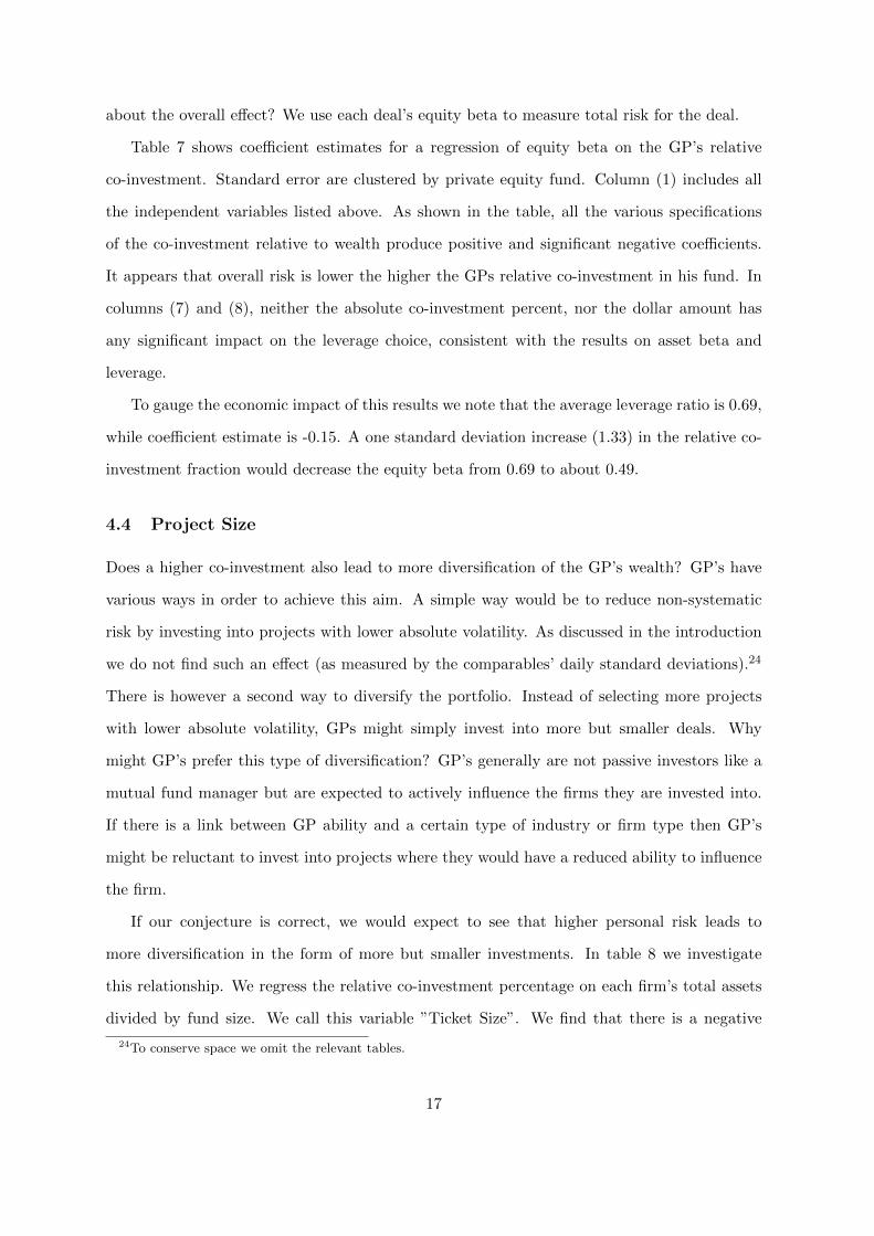
about the overall effect? We use each deal’s equity beta to measure total risk for the deal.

Table 7 shows coefficient estimates for a regression of equity beta on the GP’s relative

co-investment. Standard error are clustered by private equity fund. Column (1) includes all

the independent variables listed above. As shown in the table, all the various specifications

of the co-investment relative to wealth produce positive and significant negative coefficients.

It appears that overall risk is lower the higher the GPs relative co-investment in his fund. In

columns (7) and (8), neither the absolute co-investment percent, nor the dollar amount has

any significant impact on the leverage choice, consistent with the results on asset beta and

leverage.

To gauge the economic impact of this results we note that the average leverage ratio is 0.69,

while coefficient estimate is -0.15. A one standard deviation increase (1.33) in the relative co-

investment fraction would decrease the equity beta from 0.69 to about 0.49.

4.4 Project Size

Does a higher co-investment also lead to more diversification of the GP’s wealth? GP’s have

various ways in order to achieve this aim. A simple way would be to reduce non-systematic

risk by investing into projects with lower absolute volatility. As discussed in the introduction

we do not find such an effect (as measured by the comparables’ daily standard deviations).24

There is however a second way to diversify the portfolio. Instead of selecting more projects

with lower absolute volatility, GPs might simply invest into more but smaller deals. Why

might GP’s prefer this type of diversification? GP’s generally are not passive investors like a

mutual fund manager but are expected to actively influence the firms they are invested into.

If there is a link between GP ability and a certain type of industry or firm type then GP’s

might be reluctant to invest into projects where they would have a reduced ability to influence

the firm.

If our conjecture is correct, we would expect to see that higher personal risk leads to

more diversification in the form of more but smaller investments. In table 8 we investigate

this relationship. We regress the relative co-investment percentage on each firm’s total assets

divided by fund size. We call this variable ”Ticket Size”. We find that there is a negative

24To conserve space we omit the relevant tables.

17

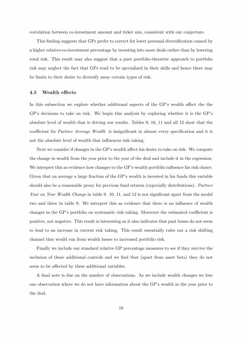
correlation between co-investment amount and ticket size, consistent with our conjecture.

This finding suggests that GPs prefer to correct for lower personal diversification caused by

a higher relative-co-investment percentage by investing into more deals rather than by lowering

total risk. This result may also suggest that a pure portfolio-theoretic approach to portfolio

risk may neglect the fact that GPs tend to be specialized in their skills and hence there may

be limits to their desire to diversify away certain types of risk.

4.5 Wealth effects

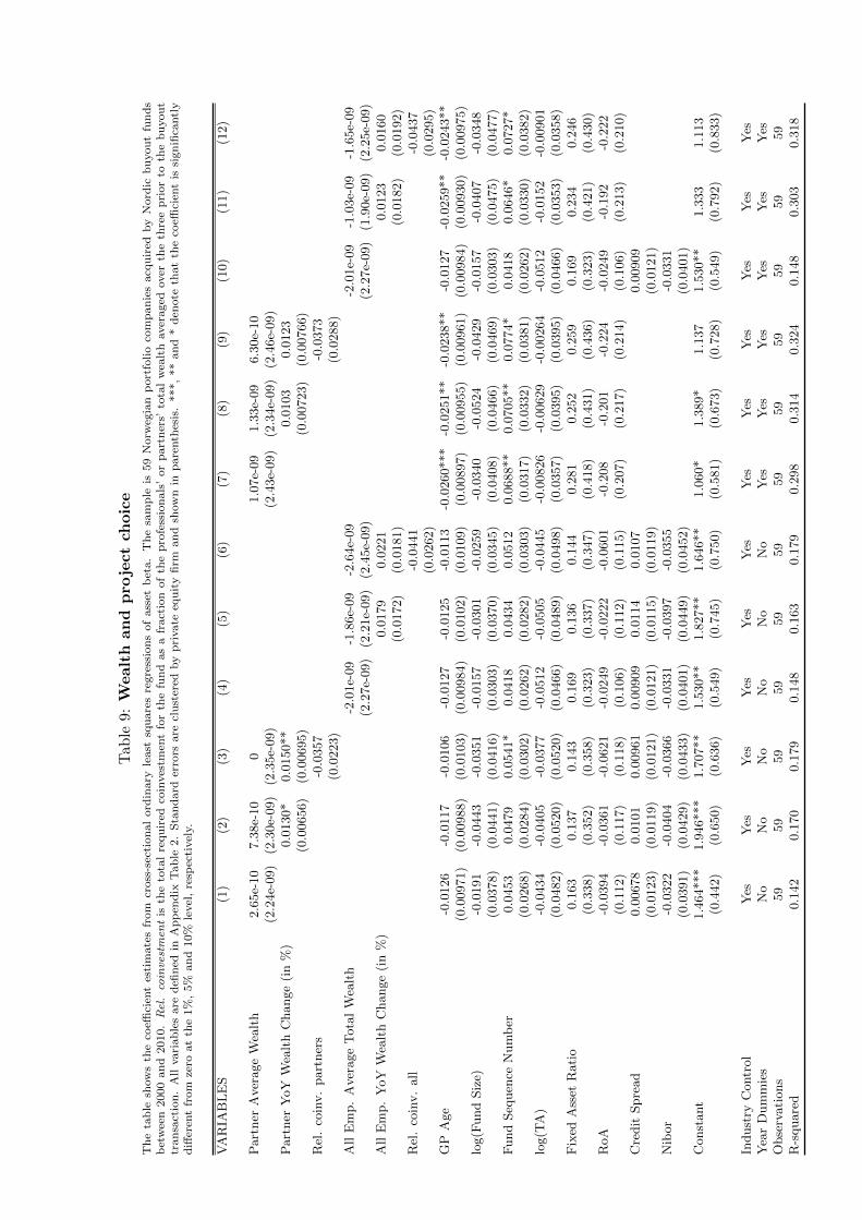
In this subsection we explore whether additional aspects of the GP’s wealth affect the the

GP’s decisions to take on risk. We begin this analysis by exploring whether it is the GP’s

absolute level of wealth that is driving our results. Tables 9, 10, 11 and all 12 show that the

coefficient for Partner Average Wealth is insignificant in almost every specification and it is

not the absolute level of wealth that influences risk taking.

Next we consider if changes in the GP’s wealth affect his desire to take on risk. We compute

the change in wealth from the year prior to the year of the deal and include it in the regression.

We interpret this as evidence how changes to the GP’s wealth portfolio influence his risk choice.

Given that on average a large fraction of the GP’s wealth is invested in his funds this variable

should also be a reasonable proxy for previous fund returns (expecially distributions). Partner

Year on Year Wealth Change in table 9. 10, 11, and 12 is not significant apart from the model

two and three in table 9. We interpret this as evidence that there is no influence of wealth

changes in the GP’s portfolio on systematic risk taking. Moreover the estimated coefficient is

positive, not negative. This result is interesting as it also indicates that past losses do not seem

to lead to an increase in current risk taking. This result essentially rules out a risk shifting

channel that would run from wealth losses to increased portfolio risk.

Finally we include our standard relative GP percentage measures to see if they survive the

inclusion of these additional controls and we find that (apart from asset beta) they do not

seem to be affected by these additional variables.

A final note is due on the number of observations. As we include wealth changes we lose

one observation where we do not have information about the GP’s wealth in the year prior to

the deal.

18

5 Conclusion

In this paper, we examine how the requirement for a co-investment by a private equity fund

manager affect his incentives to make risky investments for the fund. We first develop a model,

which predicts that a higher co-investment reduces the appetite for project risk while at the

same time increasing the appetite for leverage. We then take the model predictions to the

data, using a unique sample of Norwegian private equity transactions. The Norwegian institu-

tional setting allows us to control for the fund managers’ wealth, which may have important

implications for risk aversion.

The predictions of our model are borne out in the data. Cross-sectional regressions show

that a higher co-investment fraction is associated with less risky portfolio companies (lower

assets beta) and a higher degree of debt financing. Importantly, the co-investment fraction is

a significant determinant of investment risk only when adjusted for the fund manger’s wealth.

This emphasizes the importance of wealth data in research examining the effect of variable

compensation on the incentives to take risk.

19

References

Axelson, U., Jenkinson, T., Stromberg, P. and Weisbach, M. S. (2013). Borrow cheap,buy high? The determinants of leverage and pricing in buyouts. Journal of Finance, pp.2223–2267.

Becker, B. (2006). Wealth and executive compensation. Journal of Finance, 61, 379–397.

Bolton, P., Mehran, H. and Shapiro, J. (2011). Executive compensation and risk taking.FRB of New York Staff Report, 456.

Chung, J.-W., Sensoy, B. A., Stern, L. H. and Weisbach, M. S. (2012). Pay for perfor-mance from future fund flows: The case of private equity. Review of Financial Studies, 25,3259–3304.

Coles, J. L., Daniel, N. D. and Naveen, L. (2006). Managerial incentives and risk-taking.Journal of Financial Economics, 79, 431–468.

Colla, F. I., Paolo and Wagner, H. F. (2012). Leverage and pricing of debt in LBOs.Journal of Corporate Finance, 18, 124–137.

Driessen, J., Lin, T.-C. and Phalippou, L. (2012). A new method to estimate risk andreturn of non-traded assets from cash flows: The case of private equity funds. Journal ofFinancial and Quantitative Analysis, 47, 511–535.

Edmans, A. and Liu, Q. (2011). Inside debt. Review of Finance, 15 (1), 75–102.

Gompers, P. A. and Lerner, J. (2001). The Money of Invention: How Venture CapitalCreates New Wealth. Harvard Business Review Press.

Groh, A. P. and Gottschalg, O. (2011). The effect of leverage on the cost of capital ofUS buyouts. Journal of Banking and Finance, 35, 2099–2110.

Harris, R., Jenkinson, T. and Kaplan, S. N. (2014). Private equity performance: Whatdo we know? Journal of Finance, 69, 1851?1882.

Higson, C. and Stucke, R. (2012). The performance of private equity, working Paper,London Business School.

Jensen, M. C. (1986). Agency costs of free cash flow, corporate finance and takeovers. Amer-ican Economic Review, 76, 323–329.

Kaplan, S. N. and Schoar, A. (2005). Private equity performance: Returns, persistence,and capital flows. Journal of Finance, 60, 1791–1823.

Knopf, J. D., Nam, J. and John H. Thornton, J. (2002). The volatility and price sen-sitivities of managerial stock option portfolios and corporate hedging. Journal of Finance,58, 801–813.

Metrick, A. and Yasuda, A. (2010). The economics of private equity funds. Review ofFinancial Studies, 23, 2303–2341.

Modigliani, F. and Miller, M. H. (1958). The cost of capital, corporation finance, and thetheory of investment. American Economic Review, 48, 261–297.

20

Phalippou, L. (2009). Beware of venturing into private equity. Journal of Economic Perspec-tives, 23, 147–166.

— (2012). Performance of buyout funds revisited, working Paper, University of Oxford.

Phallipou, L. and Gottschalg, O. (2009). The performance of private equity funds. Reviewof Financial Studies, 22, 1747–1776.

Rabin, M. (2000). Risk aversion and expected-utility theory: A calibration theorem. Econo-metrica, 68 (5), 1281–1292.

Robinson, D. T. and Sensoy, B. A. (2015). Do private equity fund managers earn theirfees? Compensation, ownership, and cash flow performance. Review of Financial Studies,forthcoming.

Shue, K. and Townsend, R. (2013). Swinging for the fences: Executive reactions to quasi-random options grants, working Paper, University of Chicago.

Thanassoulis, J. (2012). The case for intervening in bankers’ pay. Journal of Finance, 67 (3),849–895.

21

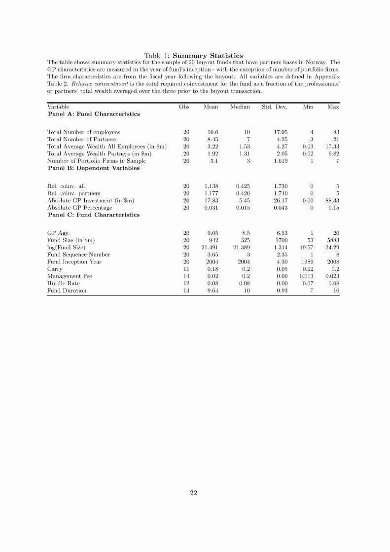
Table 1: Summary StatisticsThe table shows summary statistics for the sample of 20 buyout funds that have partners bases in Norway. TheGP characteristics are measured in the year of fund’s inception - with the exception of number of portfolio firms.The firm characteristics are from the fiscal year following the buyout. All variables are defined in AppendixTable 2. Relative coinvestment is the total required coinvestment for the fund as a fraction of the professionals’or partners’ total wealth averaged over the three prior to the buyout transaction.

Variable Obs Mean Median Std. Dev. Min MaxPanel A: Fund Characteristics

Total Number of employees 20 16.6 10 17.95 4 83Total Number of Partners 20 8.45 7 4.25 3 21Total Average Wealth All Employees (in $m) 20 3.22 1.53 4.27 0.03 17.33Total Average Wealth Partners (in $m) 20 1.92 1.31 2.05 0.02 6.82Number of Portfolio Firms in Sample 20 3.1 3 1.619 1 7Panel B: Dependent Variables

Rel. coinv. all 20 1.138 0.425 1.730 0 5Rel. coinv. partners 20 1.177 0.426 1.740 0 5Absolute GP Investment (in $m) 20 17.83 5.45 26.17 0.00 88.33Absolute GP Percentage 20 0.031 0.015 0.043 0 0.15Panel C: Fund Characteristics

GP Age 20 9.65 8.5 6.53 1 20Fund Size (in $m) 20 942 325 1700 53 5883log(Fund Size) 20 21.491 21.389 1.314 19.57 24.29Fund Sequence Number 20 3.65 3 2.35 1 8Fund Inception Year 20 2004 2004 4.30 1989 2008Carry 11 0.18 0.2 0.05 0.02 0.2Management Fee 14 0.02 0.2 0.00 0.013 0.023Hurdle Rate 12 0.08 0.08 0.00 0.07 0.08Fund Duration 14 9.64 10 0.93 7 10

22

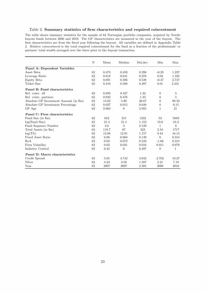
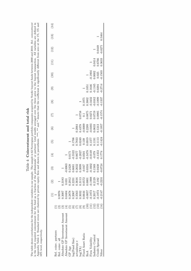
Table 2: Summary statistics of firm characteristics and required coinvestment

The table shows summary statistics for the sample of 62 Norwegian portfolio companies, acquired by Nordicbuyout funds between 2000 and 2010. The GP characteristics are measured in the year of the buyout. Thefirm characteristics are from the fiscal year following the buyout. All variables are defined in Appendix Table2. Relative coinvestment is the total required coinvestment for the fund as a fraction of the professionals’ orpartners’ total wealth averaged over the three prior to the buyout transaction.

N Mean Median Std.dev. Min Max

Panel A: Dependent VariablesAsset Beta 62 0.473 0.459 0.298 -0.29 1.237Leverage Ratio 62 0.618 0.641 0.276 0.02 1.325Equity Beta 62 0.691 0.586 0.538 -0.47 2.747Ticket Size 62 0.410 0.586 0.487 0.01 2.431

Panel B: Fund characteristicsRel. coinv. all 62 0.893 0.427 1.32 0 5Rel. coinv. partners 62 0.932 0.476 1.33 0 5Absolute GP Investment Amount (in $m) 62 13.02 5.90 20.67 0 88.33Absolute GP Investment Percentage 62 0.037 0.015 0.049 0 0.15GP Age 62 9.903 8 5.955 1 21

Panel C: Firm characteristicsFund Size (in $m) 62 652 315 1232 53 5883log(Fund Size) 62 21.3 21.4 1.152 19.6 24.3Fund Sequence Number 62 3.6 3 2.129 1 8Total Assets (in $m) 62 119.7 67 223 2.10 1717log(TA) 62 12.86 12.91 1.157 9.44 16.15Fixed Asset Ratio 62 0.08 0.004 0.149 0 0.554RoA 62 0.03 0.072 0.243 -1.66 0.315Firm Volatility 62 0.03 0.031 0.016 0.011 0.078Industry Control 62 0.42 0 0.497 0 1

Panel D: Macro characteristicsCredit Spread 62 5.65 4.742 3.042 2.702 10.27Nibor 62 4.23 3.58 1.507 2.21 7.19Year 62 2007 2007 2.285 2000 2010

23

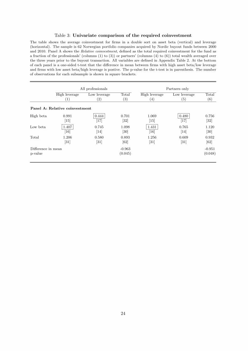
Table 3: Univariate comparison of the required coinvestment

The table shows the average coinvestment for firms in a double sort on asset beta (vertical) and leverage(horizontal). The sample is 62 Norwegian portfolio companies acquired by Nordic buyout funds between 2000and 2010. Panel A shows the Relative coinvestment, defined as the total required coinvestment for the fund asa fraction of the professionals’ (columns (1) to (3)) or partners’ (columns (4) to (6)) total wealth averaged overthe three years prior to the buyout transaction. All variables are defined in Appendix Table 2. At the bottomof each panel is a one-sided t-test that the difference in mean between firms with high asset beta/low leverageand firms with low asset beta/high leverage is postive. The p-value for the t-test is in parenthesis. The numberof observations for each subsample is shown in square brackets.

All professionals Partners only

High leverage Low leverage Total High leverage Low leverage Total(1) (2) (3) (4) (5) (6)

Panel A: Relative coinvestment

High beta 0.991 0.444 0.701 1.069 0.480 0.756[15] [17] [32] [15] [17] [32]

Low beta 1.407 0.745 1.098 1.431 0.765 1.120[16] [14] [30] [16] [14] [30]

Total 1.206 0.580 0.893 1.256 0.609 0.932[31] [31] [62] [31] [31] [62]

Difference in mean -0.963 -0.951p-value (0.045) (0.048)

24

Tab

le4:

Coin

vest

ment

an

dto

tal

risk

Th

eta

ble

show

sco

rrel

ati

on

sfo

rth

ein

dep

end

ent

vari

ab

les

inou

rsa

mp

le.

Th

esa

mp

leis

62

Norw

egia

np

ort

folio

com

pan

ies

acq

uir

edby

Nord

icb

uyou

tfu

nds

bet

wee

n2000

an

d2010.Rel.coinvestmen

tis

the

tota

lre

qu

ired

coin

ves

tmen

tfo

rth

efu

nd

as

afr

act

ion

of

the

pro

fess

ion

als

’or

part

ner

s’to

tal

wea

lth

aver

aged

over

the

thre

ep

rior

toth

eb

uyou

ttr

an

sact

ion

.A

llvari

ab

les

are

defi

ned

inA

pp

end

ixT

ab

le2.

Sta

nd

ard

erro

rsare

clu

ster

edby

pri

vate

equ

ity

firm

an

dsh

ow

nin

pare

nth

esis

.***,

**

an

d*

den

ote

that

the

coeffi

cien

tis

sign

ifica

ntl

yd

iffer

ent

from

zero

at

the

1%

,5%

an

d10%

level

,re

spec

tivel

y.

(1)

(2)

(3)

(4)

(5)

(6)

(7)

(8)

(9)

(10)

(11)

(12)

(13)

(14)

Rel

.co

inv.

part

ner

s(1

)1

Rel

.co

inv.

all

(2)

0.9

976

1A

bso

lute

GP

Inves

tmen

tA

mount

(3)

0.3

007

0.3

183

1A

bso

lute

GP

Inves

tmen

tA

mount

(4)

0.0

404

0.0

31

-0.0

063

1G

PA

ge

(5)

0.2

878

0.2

912

0.2

428

0.0

171

1lo

g(F

und

Siz

e)(6

)0.2

067

0.2

231

0.6

681

-0.5

522

0.1

706

1act

uals

equ

e(7

)0.3

563

0.3

616

0.2

632

0.0

677

0.7

833

0.2

064

1lo

g(T

A)

(8)

0.3

032

0.3

113

0.3

099

-0.2

027

0.0

249

0.4

378

0.0

758

1F

ixed

Ass

etR

ati

o(9

)0.0

644

0.0

572

-0.0

47

0.0

501

0.1

39

-0.0

009

0.1

0.1

975

1R

oA

(10)

-0.0

057

0.0

001

0.0

316

-0.3

478

0.0

919

0.2

289

0.0

875

0.3

802

0.1

051

1F

irm

Vola

tility

(11)

-0.1

873

-0.1

908

-0.1

602

-0.0

149

0.1

377

-0.0

483

0.0

271

-0.3

432

0.1

646

-0.1

804

1In

dust

ryC

ontr

ol

(12)

0.2

017

0.2

129

0.1

569

-0.0

78

0.1

191

0.0

633

0.0

719

-0.0

162

-0.1

165

0.0

002

0.0

414

1C

redit

Spre

ad

(13)

-0.1

873

-0.1

92

0.0

438

-0.1

353

0.1

113

0.1

213

0.0

985

-0.1

899

0.0

294

0.0

25

0.6

766

0.0

449

1N

ibor

(14)

-0.2

147

-0.2

231

-0.0

724

0.1

774

-0.1

424

-0.1

957

-0.1

574

-0.1

337

-0.2

714

-0.1

503

0.3

633

-0.0

271

0.5

464

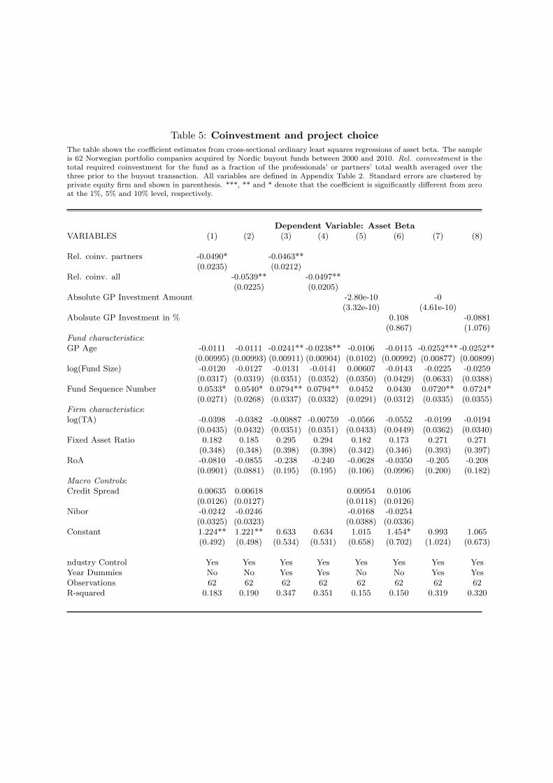
Table 5: Coinvestment and project choice

The table shows the coefficient estimates from cross-sectional ordinary least squares regressions of asset beta. The sampleis 62 Norwegian portfolio companies acquired by Nordic buyout funds between 2000 and 2010. Rel. coinvestment is thetotal required coinvestment for the fund as a fraction of the professionals’ or partners’ total wealth averaged over thethree prior to the buyout transaction. All variables are defined in Appendix Table 2. Standard errors are clustered byprivate equity firm and shown in parenthesis. ***, ** and * denote that the coefficient is significantly different from zeroat the 1%, 5% and 10% level, respectively.

Dependent Variable: Asset BetaVARIABLES (1) (2) (3) (4) (5) (6) (7) (8)

Rel. coinv. partners -0.0490* -0.0463**(0.0235) (0.0212)

Rel. coinv. all -0.0539** -0.0497**(0.0225) (0.0205)

Absolute GP Investment Amount -2.80e-10 -0(3.32e-10) (4.61e-10)

Abolsute GP Investment in % 0.108 -0.0881(0.867) (1.076)

Fund characteristics:GP Age -0.0111 -0.0111 -0.0241** -0.0238** -0.0106 -0.0115 -0.0252*** -0.0252**

(0.00995) (0.00993) (0.00911) (0.00904) (0.0102) (0.00992) (0.00877) (0.00899)log(Fund Size) -0.0120 -0.0127 -0.0131 -0.0141 0.00607 -0.0143 -0.0225 -0.0259

(0.0317) (0.0319) (0.0351) (0.0352) (0.0350) (0.0429) (0.0633) (0.0388)Fund Sequence Number 0.0533* 0.0540* 0.0794** 0.0794** 0.0452 0.0430 0.0720** 0.0724*

(0.0271) (0.0268) (0.0337) (0.0332) (0.0291) (0.0312) (0.0335) (0.0355)Firm characteristics:log(TA) -0.0398 -0.0382 -0.00887 -0.00759 -0.0566 -0.0552 -0.0199 -0.0194

(0.0435) (0.0432) (0.0351) (0.0351) (0.0433) (0.0449) (0.0362) (0.0340)Fixed Asset Ratio 0.182 0.185 0.295 0.294 0.182 0.173 0.271 0.271

(0.348) (0.348) (0.398) (0.398) (0.342) (0.346) (0.393) (0.397)RoA -0.0810 -0.0855 -0.238 -0.240 -0.0628 -0.0350 -0.205 -0.208

(0.0901) (0.0881) (0.195) (0.195) (0.106) (0.0996) (0.200) (0.182)Macro Controls:Credit Spread 0.00635 0.00618 0.00954 0.0106

(0.0126) (0.0127) (0.0118) (0.0126)Nibor -0.0242 -0.0246 -0.0168 -0.0254

(0.0325) (0.0323) (0.0388) (0.0336)Constant 1.224** 1.221** 0.633 0.634 1.015 1.454* 0.993 1.065

(0.492) (0.498) (0.534) (0.531) (0.658) (0.702) (1.024) (0.673)

ndustry Control Yes Yes Yes Yes Yes Yes Yes YesYear Dummies No No Yes Yes No No Yes YesObservations 62 62 62 62 62 62 62 62R-squared 0.183 0.190 0.347 0.351 0.155 0.150 0.319 0.320

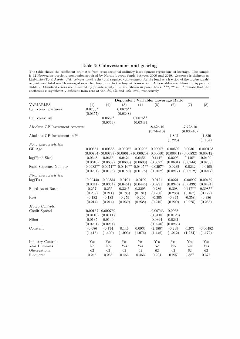
Table 6: Coinvestment and gearing

The table shows the coefficient estimates from cross-sectional ordinary least squares regressions of leverage. The sampleis 62 Norwegian portfolio companies acquired by Nordic buyout funds between 2000 and 2010. Leverage is defineds asLiabilities/Total Assets. Rel. coinvestment is the total required coinvestment for the fund as a fraction of the professionals’or partners’ total wealth averaged over the three prior to the buyout transaction. All variables are defined in AppendixTable 2. Standard errors are clustered by private equity firm and shown in parenthesis. ***, ** and * denote that thecoefficient is significantly different from zero at the 1%, 5% and 10% level, respectively.

Dependent Variable: Leverage RatioVARIABLES (1) (2) (3) (4) (5) (6) (7) (8)Rel. coinv. partners 0.0700* 0.0876**

(0.0357) (0.0348)Rel. coinv. all 0.0669* 0.0875**

(0.0363) (0.0348)Absolute GP Investment Amount -8.62e-10 -7.72e-10

(5.74e-10) (6.03e-10)Abolsute GP Investment in % -1.895 -1.339

(1.225) (1.164)Fund characteristics:GP Age 0.00561 0.00563 -0.00267 -0.00292 0.00907 0.00592 0.00361 0.000193

(0.00794) (0.00797) (0.00616) (0.00620) (0.00660) (0.00641) (0.00832) (0.00812)log(Fund Size) 0.0648 0.0666 0.0424 0.0456 0.141* 0.0295 0.140* 0.0400

(0.0610) (0.0609) (0.0608) (0.0600) (0.0697) (0.0601) (0.0744) (0.0738)Fund Sequence Number -0.0483** -0.0474** -0.0416** -0.0405** -0.0297* -0.0235 -0.0232 -0.0195

(0.0201) (0.0195) (0.0180) (0.0178) (0.0162) (0.0217) (0.0212) (0.0247)Firm characteristics:log(TA) -0.00440 -0.00354 -0.0191 -0.0199 0.0121 0.0221 -0.00992 0.00469

(0.0341) (0.0334) (0.0451) (0.0445) (0.0291) (0.0346) (0.0439) (0.0484)Fixed Asset Ratio 0.257 0.255 0.324* 0.329* 0.286 0.308 0.417** 0.398**

(0.209) (0.211) (0.183) (0.181) (0.230) (0.238) (0.167) (0.179)RoA -0.182 -0.183 -0.259 -0.260 -0.305 -0.345 -0.358 -0.386

(0.214) (0.214) (0.239) (0.238) (0.210) (0.229) (0.225) (0.255)Macro Controls:Credit Spread 0.00132 0.000759 -0.00743 -0.00681

(0.0110) (0.0111) (0.0118) (0.0126)Nibor 0.0135 0.0140 0.0394 0.0231

(0.0254) (0.0254) (0.0240) (0.0256)Constant -0.686 -0.734 0.146 0.0933 -2.580* -0.239 -1.971 -0.00482

(1.415) (1.409) (1.093) (1.076) (1.446) (1.212) (1.224) (1.172)

Industry Control Yes Yes Yes Yes Yes Yes Yes YesYear Dummies No No Yes Yes No No Yes YesObservations 62 62 62 62 62 62 62 62R-squared 0.243 0.236 0.463 0.463 0.224 0.227 0.387 0.376

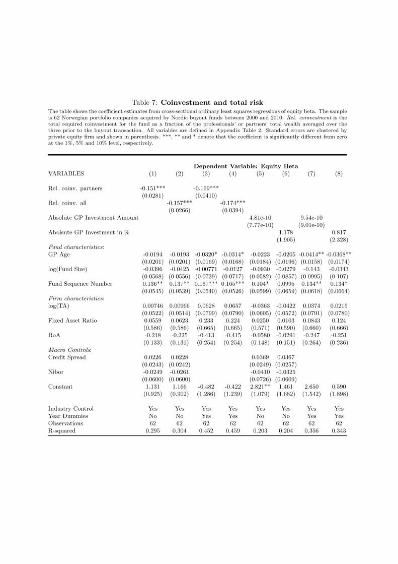
Table 7: Coinvestment and total riskThe table shows the coefficient estimates from cross-sectional ordinary least squares regressions of equity beta. The sampleis 62 Norwegian portfolio companies acquired by Nordic buyout funds between 2000 and 2010. Rel. coinvestment is thetotal required coinvestment for the fund as a fraction of the professionals’ or partners’ total wealth averaged over thethree prior to the buyout transaction. All variables are defined in Appendix Table 2. Standard errors are clustered byprivate equity firm and shown in parenthesis. ***, ** and * denote that the coefficient is significantly different from zeroat the 1%, 5% and 10% level, respectively.

Dependent Variable: Equity BetaVARIABLES (1) (2) (3) (4) (5) (6) (7) (8)

Rel. coinv. partners -0.151*** -0.169***(0.0281) (0.0410)

Rel. coinv. all -0.157*** -0.174***(0.0266) (0.0394)

Absolute GP Investment Amount 4.81e-10 9.54e-10(7.77e-10) (9.01e-10)

Abolsute GP Investment in % 1.178 0.817(1.905) (2.328)

Fund characteristics:GP Age -0.0194 -0.0193 -0.0320* -0.0314* -0.0223 -0.0205 -0.0414** -0.0368**

(0.0201) (0.0201) (0.0169) (0.0168) (0.0184) (0.0196) (0.0158) (0.0174)log(Fund Size) -0.0396 -0.0425 -0.00771 -0.0127 -0.0930 -0.0279 -0.143 -0.0343

(0.0568) (0.0556) (0.0739) (0.0717) (0.0582) (0.0857) (0.0995) (0.107)Fund Sequence Number 0.136** 0.137** 0.167*** 0.165*** 0.104* 0.0995 0.134** 0.134*

(0.0545) (0.0539) (0.0540) (0.0526) (0.0599) (0.0659) (0.0618) (0.0664)Firm characteristics:log(TA) 0.00746 0.00966 0.0628 0.0657 -0.0363 -0.0422 0.0374 0.0215

(0.0522) (0.0514) (0.0799) (0.0790) (0.0605) (0.0572) (0.0791) (0.0780)Fixed Asset Ratio 0.0559 0.0623 0.233 0.224 0.0250 0.0103 0.0843 0.124

(0.586) (0.586) (0.665) (0.665) (0.571) (0.590) (0.660) (0.666)RoA -0.218 -0.225 -0.413 -0.415 -0.0580 -0.0291 -0.247 -0.251

(0.133) (0.131) (0.254) (0.254) (0.148) (0.151) (0.264) (0.236)Macro Controls:Credit Spread 0.0226 0.0228 0.0369 0.0367

(0.0243) (0.0242) (0.0249) (0.0257)Nibor -0.0249 -0.0261 -0.0410 -0.0325

(0.0600) (0.0600) (0.0726) (0.0609)Constant 1.131 1.166 -0.482 -0.422 2.821** 1.461 2.650 0.590

(0.925) (0.902) (1.286) (1.239) (1.079) (1.682) (1.542) (1.898)

Industry Control Yes Yes Yes Yes Yes Yes Yes YesYear Dummies No No Yes Yes No No Yes YesObservations 62 62 62 62 62 62 62 62R-squared 0.295 0.304 0.452 0.459 0.203 0.204 0.356 0.343

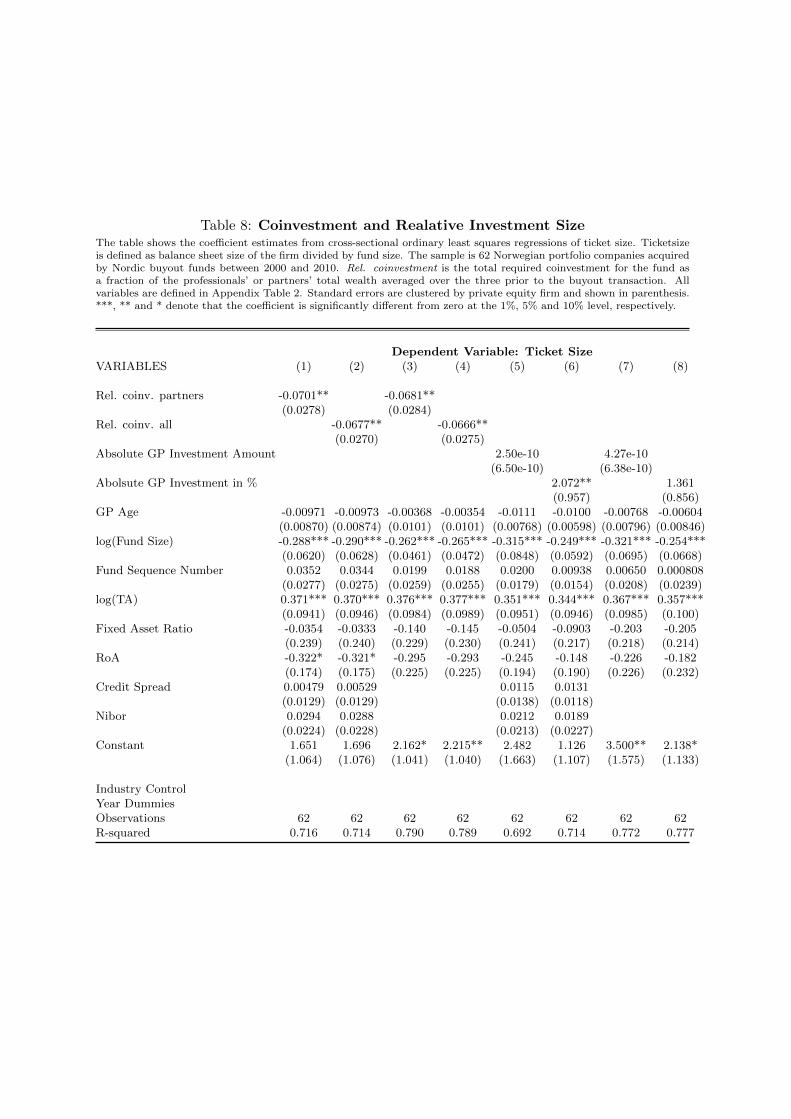
Table 8: Coinvestment and Realative Investment SizeThe table shows the coefficient estimates from cross-sectional ordinary least squares regressions of ticket size. Ticketsizeis defined as balance sheet size of the firm divided by fund size. The sample is 62 Norwegian portfolio companies acquiredby Nordic buyout funds between 2000 and 2010. Rel. coinvestment is the total required coinvestment for the fund asa fraction of the professionals’ or partners’ total wealth averaged over the three prior to the buyout transaction. Allvariables are defined in Appendix Table 2. Standard errors are clustered by private equity firm and shown in parenthesis.***, ** and * denote that the coefficient is significantly different from zero at the 1%, 5% and 10% level, respectively.

Dependent Variable: Ticket SizeVARIABLES (1) (2) (3) (4) (5) (6) (7) (8)

Rel. coinv. partners -0.0701** -0.0681**(0.0278) (0.0284)

Rel. coinv. all -0.0677** -0.0666**(0.0270) (0.0275)

Absolute GP Investment Amount 2.50e-10 4.27e-10(6.50e-10) (6.38e-10)

Abolsute GP Investment in % 2.072** 1.361(0.957) (0.856)

GP Age -0.00971 -0.00973 -0.00368 -0.00354 -0.0111 -0.0100 -0.00768 -0.00604(0.00870) (0.00874) (0.0101) (0.0101) (0.00768) (0.00598) (0.00796) (0.00846)

log(Fund Size) -0.288*** -0.290*** -0.262*** -0.265*** -0.315*** -0.249*** -0.321*** -0.254***(0.0620) (0.0628) (0.0461) (0.0472) (0.0848) (0.0592) (0.0695) (0.0668)

Fund Sequence Number 0.0352 0.0344 0.0199 0.0188 0.0200 0.00938 0.00650 0.000808(0.0277) (0.0275) (0.0259) (0.0255) (0.0179) (0.0154) (0.0208) (0.0239)

log(TA) 0.371*** 0.370*** 0.376*** 0.377*** 0.351*** 0.344*** 0.367*** 0.357***(0.0941) (0.0946) (0.0984) (0.0989) (0.0951) (0.0946) (0.0985) (0.100)

Fixed Asset Ratio -0.0354 -0.0333 -0.140 -0.145 -0.0504 -0.0903 -0.203 -0.205(0.239) (0.240) (0.229) (0.230) (0.241) (0.217) (0.218) (0.214)

RoA -0.322* -0.321* -0.295 -0.293 -0.245 -0.148 -0.226 -0.182(0.174) (0.175) (0.225) (0.225) (0.194) (0.190) (0.226) (0.232)

Credit Spread 0.00479 0.00529 0.0115 0.0131(0.0129) (0.0129) (0.0138) (0.0118)

Nibor 0.0294 0.0288 0.0212 0.0189(0.0224) (0.0228) (0.0213) (0.0227)

Constant 1.651 1.696 2.162* 2.215** 2.482 1.126 3.500** 2.138*(1.064) (1.076) (1.041) (1.040) (1.663) (1.107) (1.575) (1.133)

Industry ControlYear DummiesObservations 62 62 62 62 62 62 62 62R-squared 0.716 0.714 0.790 0.789 0.692 0.714 0.772 0.777

Tab

le9:

Wealt

han

dp

roje

ct

choic

e

Th

eta

ble

show

sth

eco

effici

ent

esti

mate

sfr

om

cross

-sec

tion

al

ord

inary

least

squ

are

sre

gre

ssio

ns

of

ass

etb

eta.

Th

esa

mp

leis

59

Norw

egia

np

ort

folio

com

pan

ies

acq

uir

edby

Nord

icb

uyou

tfu

nd

sb

etw

een

2000

an

d2010.Rel.coinvestmen

tis

the

tota

lre

qu

ired

coin

ves

tmen

tfo

rth

efu

nd

as

afr

act

ion

of

the

pro

fess

ion

als

’or

part

ner

s’to

tal

wea

lth

aver

aged

over

the

thre

ep

rior

toth

eb

uyou

ttr

an

sact

ion

.A

llvari

ab

les

are

defi

ned

inA

pp

end

ixT

ab

le2.

Sta

nd

ard

erro

rsare

clu

ster

edby

pri

vate

equ

ity

firm

an

dsh

ow

nin

pare

nth

esis

.***,

**

an

d*

den

ote

that

the

coeffi

cien

tis

sign

ifica

ntl

yd

iffer

ent

from

zero

at

the

1%

,5%

an

d10%

level

,re

spec

tivel

y.

VA

RIA

BL

ES

(1)

(2)

(3)

(4)

(5)

(6)

(7)

(8)

(9)

(10)

(11)

(12)

Part

ner

Aver

age

Wea

lth

2.6

5e-

10

7.3

8e-

10

01.0

7e-

09

1.3

3e-

09

6.3

0e-

10

(2.2

4e-

09)

(2.3

0e-

09)

(2.3

5e-

09)

(2.4

3e-

09)

(2.3

4e-

09)

(2.4

6e-

09)

Part

ner

YoY

Wea

lth

Change

(in

%)

0.0

130*

0.0

150**

0.0

103

0.0

123

(0.0

0656)

(0.0

0695)

(0.0

0723)

(0.0

0766)

Rel

.co

inv.

part

ner

s-0

.0357

-0.0

373

(0.0

223)

(0.0

288)

All

Em

p.

Aver

age

Tota

lW

ealt

h-2

.01e-

09

-1.8

6e-

09

-2.6

4e-

09

-2.0

1e-

09

-1.0

3e-

09

-1.6

5e-

09

(2.2

7e-

09)

(2.2

1e-

09)

(2.4

5e-

09)

(2.2

7e-

09)

(1.9

0e-

09)

(2.2

5e-

09)

All

Em

p.

YoY

Wea

lth

Change

(in

%)

0.0

179

0.0

221

0.0

123

0.0

160

(0.0

172)

(0.0

181)

(0.0

182)

(0.0

192)

Rel

.co

inv.

all

-0.0

441

-0.0

437

(0.0

262)

(0.0

295)

GP

Age

-0.0

126

-0.0

117

-0.0

106

-0.0

127

-0.0

125

-0.0

113

-0.0

260***

-0.0

251**

-0.0

238**

-0.0

127

-0.0

259**

-0.0

243**

(0.0

0971)

(0.0

0988)

(0.0

103)

(0.0

0984)

(0.0

102)

(0.0

109)

(0.0

0897)

(0.0

0955)

(0.0

0961)

(0.0

0984)

(0.0

0930)

(0.0

0975)

log(F

und

Siz

e)-0

.0191

-0.0

443

-0.0

351

-0.0

157

-0.0

301

-0.0

259

-0.0

340

-0.0

524

-0.0

429

-0.0

157

-0.0

407

-0.0

348

(0.0

378)

(0.0

441)

(0.0

416)

(0.0

303)

(0.0

370)

(0.0

345)

(0.0

408)

(0.0

466)

(0.0

469)

(0.0

303)

(0.0

475)

(0.0

477)

Fund

Seq

uen

ceN

um

ber

0.0

453

0.0

479

0.0

541*

0.0

418

0.0

434

0.0

512

0.0

688**

0.0

705**

0.0

774*

0.0

418

0.0

646*

0.0

727*

(0.0

268)

(0.0

284)

(0.0

302)

(0.0

262)

(0.0

282)

(0.0

303)

(0.0

317)

(0.0

332)

(0.0

381)

(0.0

262)

(0.0

330)

(0.0

382)

log(T

A)

-0.0

434

-0.0

405

-0.0

377

-0.0

512

-0.0

505

-0.0

445

-0.0

0826

-0.0

0629

-0.0

0264

-0.0

512

-0.0

152

-0.0

0901

(0.0

482)

(0.0

520)

(0.0

520)

(0.0

466)

(0.0

489)

(0.0

498)

(0.0

357)

(0.0

395)

(0.0

395)

(0.0

466)

(0.0

353)

(0.0

358)

Fix

edA

sset

Rati

o0.1

63

0.1

37

0.1

43

0.1

69

0.1

36

0.1

44

0.2

81

0.2

52

0.2

59

0.1

69

0.2

34

0.2

46

(0.3

38)

(0.3

52)

(0.3

58)

(0.3

23)

(0.3

37)

(0.3

47)

(0.4

18)

(0.4

31)

(0.4

36)

(0.3

23)

(0.4

21)

(0.4

30)

RoA

-0.0

394

-0.0

361

-0.0

621

-0.0

249

-0.0

222

-0.0

601

-0.2

08

-0.2

01

-0.2

24

-0.0

249

-0.1

92

-0.2

22

(0.1

12)

(0.1

17)

(0.1

18)

(0.1

06)

(0.1

12)

(0.1

15)

(0.2

07)

(0.2

17)

(0.2

14)

(0.1

06)

(0.2

13)

(0.2

10)

Cre

dit

Spre

ad

0.0

0678

0.0

101

0.0

0961

0.0

0909

0.0

114

0.0

107

0.0

0909

(0.0

123)

(0.0

119)

(0.0

121)

(0.0

121)

(0.0

115)

(0.0

119)

(0.0

121)

Nib

or

-0.0

322

-0.0

404

-0.0

366

-0.0

331

-0.0

397

-0.0

355

-0.0

331

(0.0

391)

(0.0

429)

(0.0

433)

(0.0

401)

(0.0

449)

(0.0

452)

(0.0

401)

Const

ant

1.4

64***

1.9

46***

1.7

07**

1.5

30**

1.8

27**

1.6

46**

1.0

60*

1.3

89*

1.1

37

1.5

30**

1.3

33

1.1

13

(0.4

42)

(0.6

50)

(0.6

36)

(0.5

49)

(0.7

45)

(0.7

50)

(0.5

81)

(0.6

73)

(0.7

28)

(0.5

49)

(0.7

92)

(0.8

33)

Indust

ryC

ontr

ol

Yes

Yes

Yes

Yes

Yes

Yes

Yes

Yes

Yes

Yes

Yes

Yes

Yea

rD

um

mie

sN

oN

oN

oN

oN

oN

oY

esY

esY

esY

esY

esY

esO

bse

rvati

ons

59

59

59

59

59

59

59

59

59

59

59

59

R-s

quare

d0.1

42

0.1

70

0.1

79

0.1

48

0.1

63

0.1

79

0.2

98

0.3

14

0.3

24

0.1

48

0.3

03

0.3

18

Tab

le10

:W

ealt

han

dG

eari

ng

Th

eta

ble

show

sth

eco

effici

ent

esti

mate

sfr

om

cross

-sec

tion

al

ord

inary

least

squ

are

sre

gre

ssio

ns

of

lever

age.

Th

esa

mp

leis

59

Norw

egia

np

ort

folio

com

pan

ies

acq

uir

edby

Nord

icb

uyou

tfu

nd

sb

etw

een

2000

an

d2010.Leverage

isd

efin

eds

as

Lia

bilit

ies/

Tota

lA

sset

s.Rel.coinvestmen

tis

the

tota

lre

qu

ired

coin

ves

tmen

tfo

rth

efu

nd

as

afr

act

ion

of

the

pro

fess

ion

als

’or

part

ner

s’to

tal

wea

lth

aver

aged

over

the

thre

ep

rior

toth

eb

uyou

ttr

an

sact

ion

.A

llvari

ab

les

are

defi

ned

inA

pp

end

ixT

ab

le2.

Sta

nd

ard

erro

rsare

clu

ster

edby

pri

vate

equ

ity

firm

an

dsh

ow

nin

pare

nth

esis

.***,

**

an

d*

den

ote

that

the

coeffi

cien

tis

sign

ifica

ntl

yd

iffer

ent

from

zero

at

the

1%

,5%

an

d10%

level

,re

spec

tivel

y.

VA

RIA

BL

ES

(1)

(2)

(3)

(4)

(5)

(6)

(7)

(8)

(9)

(10)

(11)

(12)

Part

ner

Aver

age

Wea

lth

-4.3

3e-

09*

-4.1

8e-

09*

-2.5

6e-

09

-5.1

2e-

09*

-4.9

7e-

09*

-3.1

4e-

09

(2.1

6e-

09)

(2.1

1e-

09)

(1.9

8e-

09)

(2.8

2e-

09)

(2.8

0e-

09)

(2.4

9e-

09)

Part

ner

YoY

Wea

lth

Change

(in

%)

0.0

0414

-0.0

00276

0.0

0591

0.0

00649

(0.0

0509)

(0.0

0482)

(0.0

0616)

(0.0

0591)

Rel

.co

inv.

part

ner

s0.0

807**

0.0

981***

(0.0

349)

(0.0

232)

All

Em

p.

Aver

age

Tota

lW

ealt

h-6

.05e-

09*

-5.9

4e-

09*

-4.5

6e-

09

-7.5

1e-

09**

-7.4

2e-

09**

-5.9

6e-

09**

(3.4

3e-

09)

(3.3

3e-

09)

(2.7

9e-

09)

(3.5

3e-

09)

(3.4

3e-

09)

(2.5

6e-

09)

All

Em

p.

YoY

Wea

lth

Change

(in

%)

0.0

132

0.0

0577

0.0

151

0.0

0643

(0.0

106)

(0.0

112)

(0.0

129)

(0.0

134)

Rel

.co

inv.

all

0.0

792**

0.1

03***

(0.0

312)

(0.0

200)

GP

Age

0.0

0846

0.0

0874

0.0

0620

0.0

0772

0.0

0789

0.0

0577

0.0

0152

0.0

0204

-0.0

0135

0.0

0109

0.0

0156

-0.0

0205

(0.0

0783)

(0.0

0774)

(0.0

0842)

(0.0

0720)

(0.0

0712)

(0.0

0789)

(0.0

0915)

(0.0

0910)

(0.0

0671)

(0.0

0857)

(0.0

0866)

(0.0

0579)

log(F

und

Siz

e)0.1

37**

0.1

29*

0.1

08

0.1

04*

0.0

936

0.0

860

0.1

27**

0.1

16*

0.0

910

0.0

882

0.0

774

0.0

635

(0.0

557)

(0.0

615)

(0.0

706)

(0.0

540)

(0.0

581)

(0.0

618)

(0.0

563)

(0.0

603)

(0.0

617)

(0.0

526)

(0.0

535)

(0.0

481)

Fund

Seq

uen

ceN

um

ber

-0.0

430**

-0.0

422**

-0.0

561***

-0.0

443**

-0.0

432**

-0.0

572***

-0.0

374**

-0.0

364*

-0.0

544***

-0.0

406*

-0.0

399*

-0.0

590***

(0.0

166)

(0.0

168)

(0.0

188)

(0.0

177)

(0.0

177)

(0.0

173)

(0.0

175)

(0.0

180)

(0.0

150)

(0.0

213)

(0.0

220)

(0.0

126)

log(T

A)

-0.0

0787

-0.0

0694

-0.0

133

-0.0

0271

-0.0

0214

-0.0

129

-0.0

263

-0.0

251

-0.0

348

-0.0

253

-0.0

248

-0.0

395

(0.0

334)

(0.0

350)

(0.0

352)

(0.0

296)

(0.0

317)

(0.0

338)

(0.0

463)

(0.0

489)

(0.0

484)

(0.0

447)

(0.0

476)

(0.0

492)

Fix

edA

sset

Rati

o0.3

00

0.2

92

0.2

78

0.3

17

0.2

93

0.2

77

0.3

66**

0.3

50*

0.3

32*

0.4

00**

0.3

67*

0.3

38*

(0.2

32)

(0.2

38)

(0.2

41)

(0.2

37)

(0.2

49)

(0.2

54)

(0.1

65)

(0.1

76)

(0.1

79)

(0.1

72)

(0.1

88)

(0.1

93)

RoA

-0.2

45

-0.2

44

-0.1

86

-0.2

54

-0.2

52

-0.1

84

-0.3

31

-0.3

27

-0.2

66

-0.3

33

-0.3

29

-0.2

58

(0.2

04)

(0.2

04)

(0.2

40)

(0.1

95)

(0.1

93)

(0.2

33)

(0.2

17)

(0.2

17)

(0.2

48)

(0.2

06)

(0.2

03)

(0.2

38)

Cre

dit

Spre

ad

0.0

0115

0.0

0220

0.0

0331

0.0

0224

0.0

0397

0.0

0535

(0.0

103)

(0.0

108)

(0.0

110)

(0.0

105)

(0.0

111)

(0.0

112)

Nib

or

0.0

308

0.0

282

0.0

196

0.0

282

0.0

233

0.0

159

(0.0

208)

(0.0

233)

(0.0

273)

(0.0

203)

(0.0

234)

(0.0

272)

Const

ant

-2.1

31*

-1.9

78

-1.4

38

-1.5

06

-1.2

86

-0.9

62

-1.3

72

-1.1

82

-0.5

21

-0.5

95

-0.3

85

0.1

34

(1.2

00)

(1.3

22)

(1.5

67)

(1.2

26)

(1.3

29)

(1.4

82)

(0.9

48)

(1.0

37)

(1.1

07)

(0.9

02)

(0.9

40)

(0.9

23)

Indust

ryC

ontr

ol

Yes

Yes

Yes

Yes

Yes

Yes

Yes

Yes

Yes

Yes

Yes

Yes

Macr

oC

ontr

ols

Yes

Yes

Yes

Yes

Yes

Yes

No

No

No

No

No

No

Yea

rD

um

mie

sN

oN

oN

oN

oN

oN

oY

esY

esY

esY

esY

esY

esO

bse

rvati

ons

59

59

59

59

59

59

59

59

59

59

59

59

R-s

quare

d0.2

85

0.2

88

0.3

40

0.2

84

0.2

93

0.3

49

0.4

85

0.4

91

0.5

66

0.4

96

0.5

07

0.5

97

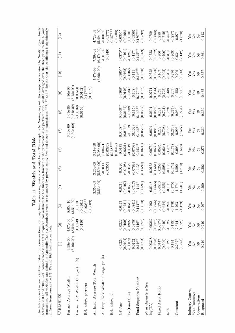
Tab

le11

:W

ealt

han

dT

ota

lR

isk

Th

eta

ble

show

sth

eco

effici

ent

esti

mate

sfr

om

cross

-sec

tion

al

ord

inary

least

squ

are

sre

gre

ssio

ns

of

equ

ity

bet

a.

Th

esa

mp

leis

59

Norw

egia

np

ort

folio

com

pan

ies

acq

uir

edby

Nord

icb

uyou

tfu

nd

sb

etw

een

2000

an

d2010.Rel.coinvestmen

tis

the

tota

lre

qu

ired

coin

ves

tmen

tfo

rth

efu

nd

as

afr

act

ion

of

the

pro

fess

ion

als

’or

part

ner

s’to

tal

wea

lth

aver

aged

over

the

thre

ep

rior

toth

eb

uyou

ttr

an

sact

ion

.A

llvari

ab

les

are

defi

ned

inA

pp

end

ixT

ab

le2.

Sta

nd

ard

erro

rsare

clu

ster

edby

pri

vate

equ

ity

firm

an

dsh

ow

nin

pare

nth

esis

.***,

**

an

d*

den

ote

that

the

coeffi

cien

tis

sign

ifica

ntl

yd

iffer

ent

from

zero

at

the

1%

,5%

an

d10%

level

,re

spec

tivel

y.

VA

RIA

BL

ES

(1)

(2)

(3)

(4)

(5)

(6)

(7)

(8)

(9)

(10)

(11)

(12)

Part

ner

Aver

age

Wea

lth

3.9

8e-

09

4.0

7e-

09

8.0

5e-

10

6.6

9e-

09

6.6

5e-

09

3.3

6e-

09

(3.4

6e-

09)

(3.5

4e-

09)

(3.5

1e-

09)

(4.3

9e-

09)

(4.3

1e-

09)

(3.7

5e-

09)

Part

ner

YoY

Wea

lth

Change

(in

%)

0.0

0249

0.0

113

-0.0

0168

0.0

0780

(0.0

150)

(0.0

161)

(0.0

156)

(0.0

162)

Rel

.co

inv.

part

ner

s-0

.162***

-0.1

77***

(0.0

509)

(0.0

562)

All

Em

p.

Aver

age

Tota

lW

ealt

h3.3

5e-

09

3.2

6e-

09

3.1

7e-

10

7.4

7e-

09

7.3

6e-

09

4.7

2e-

09

(5.5

3e-

09)

(5.5

0e-

09)

(5.0

8e-

09)

(6.6

0e-

09)

(6.4

7e-

09)

(5.4

9e-

09)

All

Em

p.

YoY

Wea

lth

Change

(in

%)

-0.0

111

0.0

0471

-0.0

174

-0.0

0169

(0.0

355)

(0.0

386)

(0.0

349)

(0.0

377)

Rel

.co

inv.

all

-0.1

68***

-0.1

87***

(0.0

442)

(0.0

503)

GP

Age

-0.0

224

-0.0

222

-0.0

171

-0.0

219

-0.0

220

-0.0

175

-0.0

368**

-0.0

369**

-0.0

308*

-0.0

365**

-0.0

370**

-0.0

305*

(0.0

194)

(0.0

199)

(0.0

221)

(0.0

197)

(0.0

198)

(0.0

221)

(0.0

165)

(0.0

167)

(0.0

176)

(0.0

162)

(0.0

161)

(0.0

168)

log(F

und

Siz

e)-0

.0879

-0.0

927

-0.0

510

-0.0

568

-0.0

479

-0.0

319

-0.0

819

-0.0

789

-0.0

337

-0.0

368

-0.0

243

0.0

0101

(0.0

752)

(0.0

878)

(0.0

841)

(0.0

717)

(0.0

788)

(0.0

709)

(0.1

02)

(0.1

15)

(0.1

08)

(0.1

11)

(0.1

17)

(0.0

956)

Fund

Seq

uen

ceN

um

ber

0.1

16*

0.1

16*

0.1

44**

0.1

14*

0.1

13*

0.1

43**

0.1

46**

0.1

46**

0.1

79**

0.1

46**

0.1

45**

0.1

80***

(0.0

593)

(0.0

597)

(0.0

613)

(0.0

597)

(0.0

589)

(0.0

600)

(0.0

556)

(0.0

557)

(0.0

637)

(0.0

570)

(0.0

559)

(0.0

592)

Firm

characteristics

:lo

g(T

A)

-0.0

0318

-0.0

0262

0.0

102

-0.0

148

-0.0

153

0.0

0750

0.0

604

0.0

601

0.0

774

0.0

528

0.0

523

0.0

789

(0.0

578)

(0.0

587)

(0.0

555)

(0.0

556)

(0.0

561)

(0.0

539)

(0.0

859)

(0.0

869)

(0.0

844)

(0.0

856)

(0.0

872)

(0.0

863)

Fix

edA

sset

Rati

o0.0

147

0.0

0974

0.0

374

0.0

0510

0.0

256

0.0

585

0.2

22

0.2

27

0.2

59

0.1

67

0.2

06

0.2

58

(0.5

99)

(0.6

10)

(0.6

24)

(0.5

85)

(0.5

95)

(0.6

24)

(0.7

08)

(0.7

21)

(0.7

25)

(0.6

95)

(0.7

06)

(0.7

19)

RoA

-0.1

27

-0.1

26

-0.2

44

-0.1

06

-0.1

08

-0.2

52

-0.3

27

-0.3

28

-0.4

38

-0.3

14

-0.3

19

-0.4

49*

(0.1

74)

(0.1

79)

(0.1

76)

(0.1

75)

(0.1

74)

(0.1

71)

(0.2

73)

(0.2

74)

(0.2

67)

(0.2

76)

(0.2

69)

(0.2

57)

Const

ant

2.2

52*

2.3

44

1.2

63

1.7

74

1.5

90

0.9

03

0.9

93

0.9

39

-0.2

52

0.2

09

-0.0

344

-0.9

76

(1.2

73)

(1.5

92)

(1.4

79)

(1.5

01)

(1.7

10)

(1.5

48)

(1.5

27)

(1.8

54)

(1.8

66)

(1.9

13)

(2.1

42)

(1.8

70)

Indust

ryC

ontr

ol

Yes

Yes

Yes

Yes

Yes

Yes

Yes

Yes

Yes

Yes

Yes

Yes

Yea

rD

um

mie

sN

oN

oN

oN

oN

oN

oY

esY

esY

esY

esY

esY

esO

bse

rvati

ons

59

59

59

59

59

59

59

59

59

59

59

59

R-s

quare

d0.2

10

0.2

10

0.2

67

0.2

00

0.2

02

0.2

71

0.3

69

0.3

69

0.4

35

0.3

57

0.3

61

0.4

43

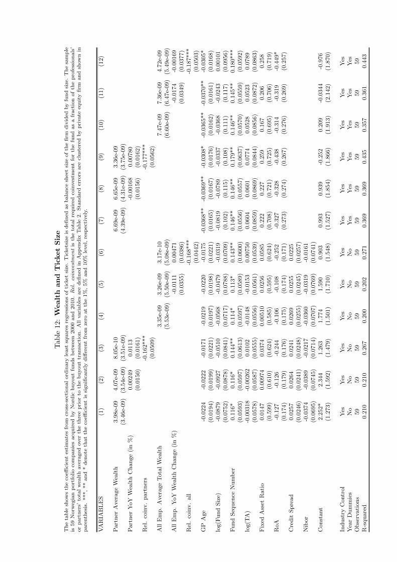
Tab

le12

:W

ealt

han

dT

icket

Siz

eT

he

tab

lesh

ow

sth

eco

effici

ent

esti

mate

sfr

om

cross

-sec

tion

al

ord

inary

least

squ

are

sre

gre

ssio

ns

of

tick

etsi

ze.

Tic

ket

size

isd

efin

edas

bala

nce

shee

tsi

zeof

the

firm

div

ided

by

fun

dsi

ze.

Th

esa

mp

leis

59

Norw

egia

np

ort

folio

com

pan

ies

acq

uir

edby

Nord

icb

uyou

tfu

nd

sb

etw

een

2000

an

d2010.Rel.coinvestmen

tis

the

tota

lre

qu

ired

coin

ves

tmen

tfo

rth

efu

nd

as

afr

act

ion

of

the

pro

fess

ion

als

’or

part

ner

s’to

tal

wea

lth

aver

aged

over

the

thre

ep

rior

toth

eb

uyou

ttr

an

sact

ion

.A

llvari

ab

les

are

defi

ned

inA

pp

end

ixT

ab

le2.

Sta

nd

ard

erro

rsare

clu

ster

edby

pri

vate

equ

ity

firm

an

dsh

ow

nin

pare

nth

esis

.***,

**

an

d*

den

ote

that

the

coeffi

cien

tis

sign

ifica

ntl

yd

iffer

ent

from

zero

at

the

1%

,5%

an

d10%

level

,re

spec

tivel

y.

VA

RIA

BL

ES

(1)

(2)

(3)

(4)

(5)

(6)

(7)

(8)

(9)

(10)

(11)

(12)

Part

ner

Aver

age

Wea

lth

3.9

8e-

09

4.0

7e-

09

8.0

5e-

10

6.6

9e-

09

6.6

5e-

09

3.3

6e-

09

(3.4

6e-

09)

(3.5

4e-

09)

(3.5

1e-

09)

(4.3

9e-

09)

(4.3

1e-

09)

(3.7

5e-

09)

Part

ner

YoY

Wea

lth

Change

(in

%)

0.0

0249

0.0

113

-0.0

0168

0.0

0780

(0.0

150)

(0.0

161)

(0.0

156)

(0.0

162)

Rel

.co

inv.

part

ner

s-0

.162***

-0.1

77***

(0.0

509)

(0.0

562)

All

Em

p.

Aver

age

Tota

lW

ealt

h3.3

5e-

09

3.2

6e-

09

3.1

7e-

10

7.4

7e-

09

7.3

6e-

09

4.7

2e-

09

(5.5

3e-

09)

(5.5

0e-

09)

(5.0

8e-

09)

(6.6

0e-

09)

(6.4

7e-

09)

(5.4

9e-

09)

All

Em

p.

YoY

Wea

lth

Change

(in

%)

-0.0

111

0.0

0471

-0.0

174

-0.0

0169

(0.0

355)

(0.0

386)

(0.0

349)

(0.0

377)

Rel

.co

inv.

all

-0.1

68***

-0.1

87***

(0.0

442)

(0.0

503)

GP

Age

-0.0

224

-0.0

222

-0.0

171

-0.0

219

-0.0

220

-0.0

175

-0.0

368**

-0.0

369**

-0.0

308*

-0.0

365**

-0.0

370**

-0.0

305*

(0.0

194)

(0.0

199)

(0.0

221)

(0.0

197)

(0.0

198)

(0.0

221)

(0.0

165)

(0.0

167)

(0.0

176)

(0.0

162)

(0.0

161)

(0.0

168)

log(F

und

Siz

e)-0

.0879

-0.0

927

-0.0

510

-0.0

568

-0.0

479

-0.0

319

-0.0

819

-0.0

789

-0.0

337

-0.0

368

-0.0

243

0.0

0101

(0.0

752)

(0.0

878)

(0.0

841)

(0.0

717)

(0.0

788)

(0.0

709)

(0.1

02)

(0.1

15)

(0.1

08)

(0.1

11)

(0.1

17)

(0.0

956)

Fund

Seq

uen

ceN

um

ber

0.1

16*

0.1

16*

0.1

44**

0.1

14*

0.1

13*

0.1

43**

0.1

46**

0.1

46**

0.1

79**

0.1

46**

0.1

45**

0.1

80***

(0.0

593)

(0.0

597)

(0.0

613)

(0.0

597)

(0.0

589)

(0.0

600)

(0.0

556)

(0.0

557)

(0.0

637)

(0.0

570)

(0.0

559)

(0.0

592)

log(T

A)

-0.0

0318

-0.0

0262

0.0

102

-0.0

148

-0.0

153

0.0

0750

0.0

604

0.0

601

0.0

774

0.0

528

0.0

523

0.0

789

(0.0

578)

(0.0

587)

(0.0

555)

(0.0

556)

(0.0

561)

(0.0

539)

(0.0

859)

(0.0

869)

(0.0

844)

(0.0

856)

(0.0

872)

(0.0

863)

Fix

edA

sset

Rati

o0.0

147

0.0

0974

0.0

374

0.0

0510

0.0

256

0.0

585

0.2

22

0.2

27

0.2

59

0.1

67

0.2

06

0.2

58

(0.5

99)

(0.6

10)

(0.6

24)

(0.5

85)

(0.5

95)

(0.6

24)

(0.7

08)

(0.7

21)

(0.7

25)

(0.6

95)

(0.7

06)

(0.7

19)

RoA

-0.1

27

-0.1

26

-0.2

44

-0.1

06

-0.1

08

-0.2

52

-0.3

27

-0.3

28

-0.4

38

-0.3

14

-0.3

19

-0.4

49*

(0.1

74)

(0.1

79)

(0.1

76)

(0.1

75)

(0.1

74)

(0.1

71)

(0.2

73)

(0.2

74)

(0.2

67)

(0.2

76)

(0.2

69)

(0.2

57)

Cre

dit

Spre

ad

0.0

257

0.0

264

0.0

241

0.0

269

0.0

255

0.0

225

(0.0

246)

(0.0

241)

(0.0

248)

(0.0

255)

(0.0

245)

(0.0

257)

Nib

or

-0.0

374

-0.0

389

-0.0

217

-0.0

360

-0.0

319

-0.0

161

(0.0

695)

(0.0

745)

(0.0

714)

(0.0

707)

(0.0

769)

(0.0

741)

Const

ant

2.2

52*

2.3

44

1.2

63

1.7

74

1.5

90

0.9

03

0.9

93

0.9

39

-0.2

52

0.2

09

-0.0

344

-0.9

76

(1.2

73)

(1.5

92)

(1.4

79)

(1.5

01)

(1.7

10)

(1.5

48)

(1.5

27)

(1.8

54)

(1.8

66)

(1.9

13)

(2.1

42)

(1.8

70)

Indust

ryC

ontr

ol

Yes

Yes

Yes

Yes

Yes

Yes

Yes

Yes

Yes

Yes

Yes

Yes

Yea

rD

um

mie

sN

oN

oN

oN

oN

oN

oY

esY

esY

esY

esY

esY

esO

bse

rvati

ons

59

59

59

59

59

59

59

59

59

59

59

59

R-s

quare

d0.2

10

0.2

10

0.2

67

0.2

00

0.2

02

0.2

71

0.3

69

0.3

69

0.4

35

0.3

57

0.3

61

0.4

43

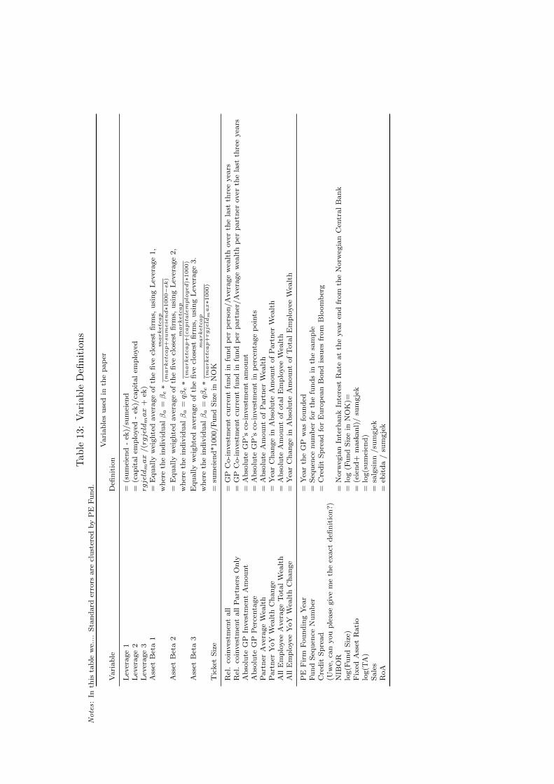
Tab

le13:

Var

iab

leD

efin

itio

ns

Notes:

Inth

ista

ble

we.

...

Sta

nd

ard

erro

rsare

clu

ster

edby

PE

Fu

nd

.

Vari

ab

les

use

din

the

pap

erV

ari

ab

leD

efin

itio

n

Lev

erage

1=

(su

mei

end

-ek

)/su

mei

end

Lev

erage

2=

(cap

ital

emp

loyed

-ek

)/ca

pit

al

emp

loyed

Lev

erage

3rgjeldmax

/(rgjeldmax

+ek

)A

sset

Bet

a1

=E

qu

ally

wei

ghte

daver

age

of

the

five

close

stfi

rms,

usi

ng

Lev

erage

1,

wh

ere

the

ind

ivid

ualβa

=βe∗

marketcap

(marketcap+sumeiend∗1

000−ek)

Ass

etB

eta

2=

Equ

ally

wei

ghte

daver

age

of

the

five

close

stfi

rms,

usi

ng

Lev

erage

2,

wh

ere

the

ind

ivid

ualβa

=qβe∗

marketcap

(marketcap+(capitalemployed)∗

1000)

Ass

etB

eta

3E

qu

ally

wei

ghte

daver

age

of

the

five

close

stfi

rms,

usi

ng

Lev

erage

3.

wh

ere

the

ind

ivid

ualβa

=qβe∗

marketcap

(marketcap+rgjeld

max∗1

000)

Tic

ket

Siz

e=

sum

eien

d*1000/F

un

dS

ize

inN

OK

Rel

.co

inves

tmen

tall

=G

PC

o-i

nves

tmen

tcu

rren

tfu

nd

infu

nd

per

per

son

/A

ver

age

wea

lth

over

the

last

thre

eyea

rsR

el.

coin

ves

tmen

tall

Part

ner

sO

nly

=G

PC

o-i

nves

tmen

tcu

rren

tfu

nd

infu

nd

per

part

ner

/A

ver

age

wea

lth

per

part

ner

over

the

last

thre

eyea

rsA

bso

lute

GP

Inves

tmen

tA

mou

nt

=A

bso

lute

GP

’sco

-inves

tmen

tam

ou

nt

Ab

solu

teG

PP

erce

nta

ge

=A

bso

lute

GP

’sco

-inves

tmen

tin

per

centa

ge

poin

tsP

art

ner

Aver

age

Wea

lth

=A

bso

lute

Am

ou

nt

of

Part

ner

Wea

lth

Part

ner

YoY

Wea

lth

Ch

an

ge

=Y

ear

Ch

an

ge

inA

bso

lute

Am

ou

nt

of

Part

ner

Wea

lth

All

Em

plo

yee

Aver

age

Tota

lW

ealt

h=

Ab

solu

teA

mou

nt

of

ota

lE

mp

loyee

Wea

lth

All

Em

plo

yee

YoY

Wea

lth

Ch

an

ge

=Y

ear

Ch

an

ge

inA

bso

lute

Am

ou

nt

of

Tota

lE

mp

loyee

Wea

lth

PE

Fir

mF

ou

nd

ing

Yea

r=

Yea

rth

eG

Pw

as

fou

nd

edF

un

dS

equ

ence

Nu

mb

er=

Seq

uen

cenu

mb

erfo

rth

efu

nd

sin

the

sam

ple

Cre

dit

Sp

read

=C

red

itS

pre

ad

for

Eu

rop

ean

Bon

dis

sues

from

Blo

om

ber

g(U

we,

can

you

ple

ase

giv

em

eth

eex

act

defi

nit

ion

?)

NIB

OR

=N

orw

egia

nIn

terb

an

kIn

tere

stR

ate

at

the

yea

ren

dfr

om

the

Norw

egia

nC

entr

al

Ban

klo

g(F

un

dS

ize)

=lo

g(F

un

dS

ize

inN

OK

)=F

ixed

Ass

etR

ati

o=

(eie

nd

+m

ask

an

l)/

sum

gje

klo

g(T

A)

=lo

g(s

um

eien

d)

Sale

s=

salg

sin

n/su

mgje

kR

oA

=eb

itd

a/

sum

gje

k

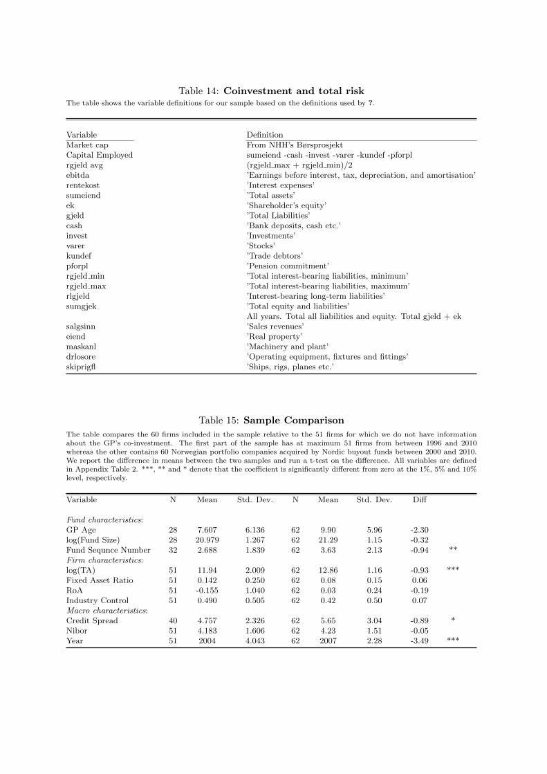
Table 14: Coinvestment and total riskThe table shows the variable definitions for our sample based on the definitions used by ?.

Variable DefinitionMarket cap From NHH’s BørsprosjektCapital Employed sumeiend -cash -invest -varer -kundef -pforplrgjeld avg (rgjeld max + rgjeld min)/2ebitda ’Earnings before interest, tax, depreciation, and amortisation’rentekost ’Interest expenses’sumeiend ’Total assets’ek ’Shareholder’s equity’gjeld ’Total Liabilities’cash ’Bank deposits, cash etc.’invest ’Investments’varer ’Stocks’kundef ’Trade debtors’pforpl ’Pension commitment’rgjeld min ’Total interest-bearing liabilities, minimum’rgjeld max ’Total interest-bearing liabilities, maximum’rlgjeld ’Interest-bearing long-term liabilities’sumgjek ’Total equity and liabilities’

All years. Total all liabilities and equity. Total gjeld + eksalgsinn ’Sales revenues’eiend ’Real property’maskanl ’Machinery and plant’drlosore ’Operating equipment, fixtures and fittings’skiprigfl ’Ships, rigs, planes etc.’

Table 15: Sample Comparison

The table compares the 60 firms included in the sample relative to the 51 firms for which we do not have informationabout the GP’s co-investment. The first part of the sample has at maximum 51 firms from between 1996 and 2010whereas the other contains 60 Norwegian portfolio companies acquired by Nordic buyout funds between 2000 and 2010.We report the difference in means between the two samples and run a t-test on the difference. All variables are definedin Appendix Table 2. ***, ** and * denote that the coefficient is significantly different from zero at the 1%, 5% and 10%level, respectively.

Variable N Mean Std. Dev. N Mean Std. Dev. Diff

Fund characteristics:GP Age 28 7.607 6.136 62 9.90 5.96 -2.30log(Fund Size) 28 20.979 1.267 62 21.29 1.15 -0.32Fund Sequnce Number 32 2.688 1.839 62 3.63 2.13 -0.94 **Firm characteristics:log(TA) 51 11.94 2.009 62 12.86 1.16 -0.93 ***Fixed Asset Ratio 51 0.142 0.250 62 0.08 0.15 0.06RoA 51 -0.155 1.040 62 0.03 0.24 -0.19Industry Control 51 0.490 0.505 62 0.42 0.50 0.07Macro characteristics:Credit Spread 40 4.757 2.326 62 5.65 3.04 -0.89 *Nibor 51 4.183 1.606 62 4.23 1.51 -0.05Year 51 2004 4.043 62 2007 2.28 -3.49 ***