face detection using discriminating feature analysis and support vector machine

Pattern Recognition 39 (2006) 260–276www.elsevier.com/locate/patcog

Face detection using discriminating feature analysisand SupportVector Machine

Peichung Shih∗, Chengjun LiuDepartment of Computer Science, New Jersey Institute of Technology, Newark, NJ 07102, USA

Received 21 September 2004; received in revised form 6 July 2005; accepted 6 July 2005

Abstract

This paper presents a novel face detection method by applying discriminating feature analysis (DFA) and support vector machine (SVM).The novelty of our DFA–SVM method comes from the integration of DFA, face class modeling, and SVM for face detection. First, DFAderives a discriminating feature vector by combining the input image, its 1-D Haar wavelet representation, and its amplitude projections.While the Haar wavelets produce an effective representation for object detection, the amplitude projections capture the vertical symmetricdistributions and the horizontal characteristics of human face images. Second, face class modeling estimates the probability density functionof the face class and defines a distribution-based measure for face and nonface classification. The distribution-based measure thus separatesthe input patterns into three classes: the face class (patterns close to the face class), the nonface class (patterns far away from the faceclass), and the undecided class (patterns neither close to nor far away from the face class). Finally, SVM together with the distribution-based measure classifies the patterns in the undecided class into either the face class or the nonface class. Experiments using images fromthe MIT–CMU test sets demonstrate the feasibility of our new face detection method. In particular, when using 92 images (containing282 faces) from the MIT–CMU test sets, our DFA–SVM method achieves 98.2% correct face detection rate with two false detections.� 2005 Pattern Recognition Society. Published by Elsevier Ltd. All rights reserved.

Keywords: Discriminating feature analysis (DFA); Distribution-based measure; Face detection; Support Vector Machine (SVM); The DFA–SVM method

1. Introduction

Face detection methods generally learns statistical mod-els of face and nonface images, and then apply two-classclassification rules to discriminate between face and non-face patterns [1,2]. As a face must be located and extractedbefore it can be verified or identified, face detection is thefirst step towards building an automated face verification oridentification system. Face verification mainly concerns au-thenticating a claimed identity posed by a person, while faceidentification focuses on recognizing the identity of a personfrom a database of known individuals [3,4]. An automatedvision system that performs the functions of face detection,verification, and identification has great potential in a wide

∗ Corresponding author.E-mail address: [email protected] (P. Shih).

0031-3203/$30.00 � 2005 Pattern Recognition Society. Published by Elsevier Ltd. All rights reserved.doi:10.1016/j.patcog.2005.07.003

spectrum of applications, such as airport security and ac-cess control, building (embassy) surveillance and monitor-ing, human–computer intelligent interaction and perceptualinterfaces, smart environments for home, office, and cars[2,1,5–7].

This paper presents a novel face detection method byapplying discriminating feature analysis (DFA) and SupportVector Machine (SVM). The novelty of our DFA–SVMmethod comes from the integration of DFA, face classmodeling, and SVM for face detection. Our DFA–SVMmethod works as follows: First, DFA derives a discriminat-ing feature vector by combining the input image, its 1-DHaar wavelet representation, and its amplitude projections.While the Haar wavelets produce an effective representationfor object detection, the amplitude projections capture thevertical symmetric distributions and the horizontal charac-teristics of human face images. Second, face class modeling

http://www.elsevier.com/locate/patcog

mailto:[email protected]

P. Shih, C. Liu / Pattern Recognition 39 (2006) 260–276 261

statistically estimates the probability density function (PDF)of the face class and defines a distribution-based measure forface and nonface classification. The face class is modeled asa multivariate normal distribution [8], and the distribution-based measure then separates the input patterns into threeclasses: the face class (patterns close to the face class), thenonface class (patterns far away from the face class), andthe undecided class (patterns neither close to nor far awayfrom the face class). Note that the distribution-based mea-sure also derives nonface patterns for SVM training. Finally,the SVM together with the distribution-based measure clas-sifies the patterns in the undecided class into either the faceclass or the nonface class. Experiments using images fromthe MIT–CMU test sets show the feasibility of our new facedetection method. The DFA–SVM method is trained using600 FERET facial images [9] and 3813 nonface images thatlie close to the face class. When tested using 92 images(containing 282 faces) from the MIT–CMU test sets [10],our DFA–SVM method achieves 98.2% correct face detec-tion rate with two false detections, a performance compa-rable to the state-of-the-art face detection methods, such asSchneiderman–Kanade’s method [11].

2. Background

Earlier efforts of face detection research have beenfocused on correlation or template matching, matchedfiltering, subspace methods, deformable templates, etc.[12,13]. For comprehensive surveys of these early meth-ods, see Refs. [14,6,7]. Recent face detection approaches,however, emphasize on statistical modeling and machinelearning techniques [15,16]. Some representative methodsare the probabilistic visual learning method [8], the example-based learning method [17], the neural network-basedlearning method [10,18], the probabilistic modeling method[11,19], the mixture of linear subspaces method [20], themachine learning approach using a boosted cascade of sim-ple features [21], statistical learning theory and SVM-basedmethods [22–24], the Markov random field-based methods[25,26], the color-based face detection method [27], and theBayesian discriminating feature (BDF) method [28].

Moghaddam and Pentland [8] applied unsupervised learn-ing to estimate the density in a high-dimensional eigenspaceand derived a maximum likelihood method for single facedetection. Rather than using principal component analysis(PCA) for dimensionality reduction, they implemented theeigenspace decomposition as an integral part of estimat-ing the conditional PDF in the original high-dimensionalimage space. Face detection is then carried out by com-puting multiscale saliency maps based on the maximumlikelihood formulation. Sung and Poggio [17] presented anexample-based learning method by means of modeling thedistributions of face and nonface patterns. To cope withthe variability of face images, they empirically chose sixGaussian clusters to model the distributions for face andnonface patterns, respectively. The density functions of the

distributions are then fed to a multiple layer perceptronfor face detection. Rowley et al. [10] developed a neuralnetwork-based upright, frontal face detection system, whichapplies a retinally connected neural network to examinesmall windows of an image and decide whether each windowcontains a face. The face detector, which was trained using alarge number of face and nonface examples, contains a set ofneural network-based filters and an arbitrator which mergesdetections from individual filters and eliminates overlappingdetections. In order to detect faces at any degree of rotationin the image plane, the system was extended to incorporatea separate router network, which determines the orientationof the face pattern. The pattern is then derotated back to theupright position, which can be processed by the early devel-oped system [18]. Schneiderman and Kanade [19] proposeda face detector based on the estimation of the posterior prob-ability function, which captures the joint statistics of localappearance and position as well as the statistics of local ap-pearance in the visual world. To detect side views of a face,profile images were added to the training set to incorporatesuch statistics [11]. Viola and Jones [21] presented a ma-chine learning approach for face detection. The novelty oftheir approach comes from the integration of a new imagerepresentation (integral image), a learning algorithm (basedon AdaBoost), and a method for combining classifiers (cas-cade). Hsu et al. [27] developed a face detection method incolor images by detecting skin regions first, and then gen-erating face candidates based on some constraints, such asthe spatial arrangement. The face candidates are further ver-ified by constructing eye, mouth, and boundary maps. Liu[28] recently developed a BDF method for multiple frontalface detection. The BDF method applies a DFA procedurefor image representation, statistical modeling of face andnonface classes, and the Bayes classifier for face detection.

SVM is a particular implementation of statistical learn-ing theory, which describes an approach known as struc-tural risk minimization by minimizing the risk functional interms of both the empirical risk and the confidence inter-val [29]. Osuna et al. [30] pioneered the research of facedetection using SVM and demonstrated its generalizationcapability for face detection. Papageorgiou et al. [31] de-veloped a wavelet-based SVM method for face and pedes-trian detection. Romdhani et al. [32] proposed a method forspeeding up a nonlinear SVM by evaluating a subset of sup-port vectors. Recently, Bartlett et al. [33] combined an Ad-aBoost algorithm with an SVM for face detection in video,and Heisele et al. [34] presented a hierarchical face detec-tion method using cascaded SVMs for face detection in acoarse-to-fine fashion.

3. Face detection using discriminating feature analysisand Support Vector Machine

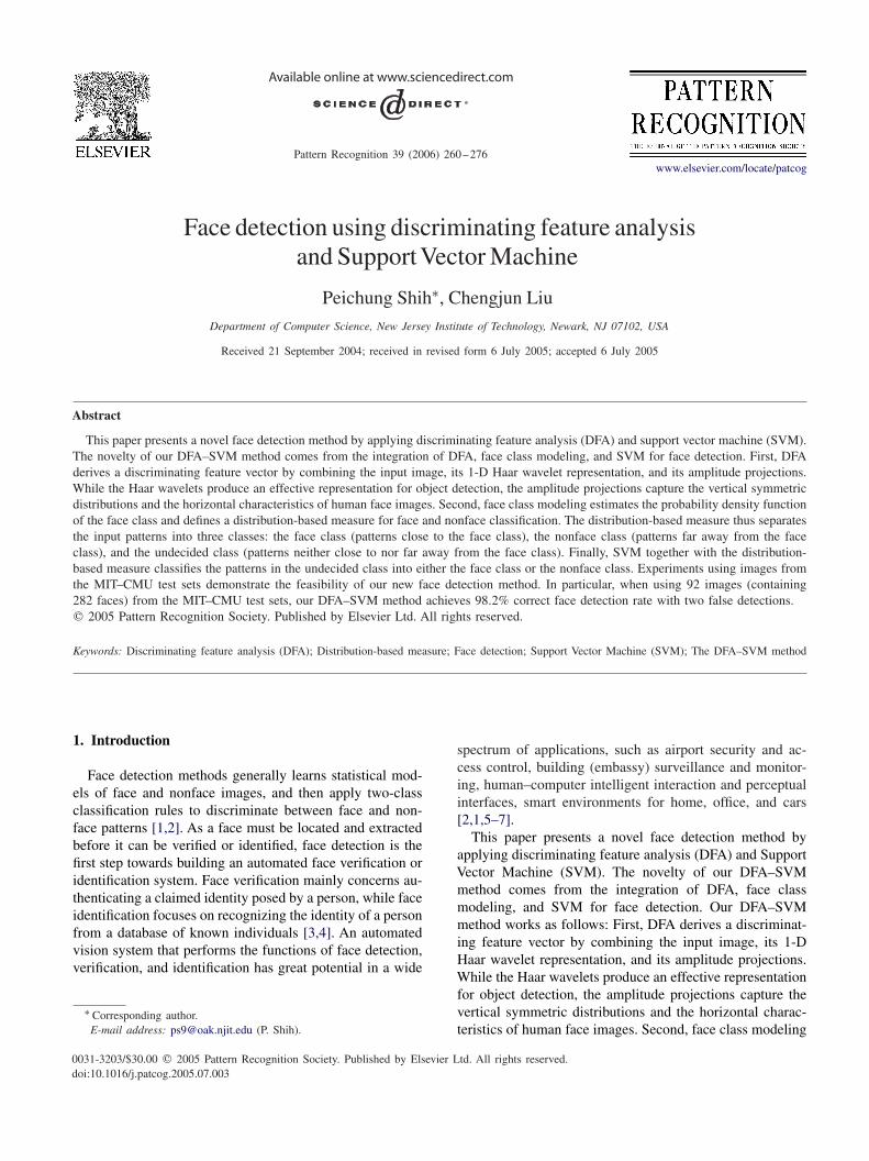
The system architecture of our DFA–SVM face detectionmethod is shown in Fig. 1. An input image is first processedby the DFA, which defines a feature vector by combining

262 P. Shih, C. Liu / Pattern Recognition 39 (2006) 260–276

DFA

Undecided Class

Face Class Nonface Class

Measure

SVM

DFA-SVM

Fig. 1. System architecture of the DFA–SVM face detection method.

the input image, its 1-D Haar wavelet representation, andits amplitude projections. Based on the DFA feature vector,the face class is then modeled using a multivariate normaldensity and a distribution-based measure is defined for faceand nonface classification. The distribution-based measureseparates the patterns in the input image into three classes:the face class (patterns close to the face class), the nonfaceclass (patterns far away from the face class), and the unde-cided class (patterns neither close to nor far away from theface class). Finally, a SVM detects faces in the undecidedclass and passes patterns to the DFA–SVM decision rule,which further classifies them into either the face class or thenonface class.

3.1. Discriminating feature analysis

Let I (i, j) ∈ Rm×n represent an input image (e.g., train-ing images for the face and the nonface classes, or subim-ages of test images), and X ∈ Rmn be the vector formedby concatenating the rows (or columns) of I (i, j). The 1-DHaar representation of I (i, j) yields two images, Ih(i, j) ∈R(m−1)×n and Iv(i, j) ∈ Rm×(n−1), corresponding to thehorizontal and vertical difference images, respectively.Ih(i, j) and Iv(i, j) then form two vectors, Xh ∈ R(m−1)n

and Xv ∈ Rm(n−1), by concatenating the rows (or columns).The amplitude projections of I (i, j) along its rows andcolumns form the horizontal (row) and vertical (column)projections, Xr ∈ Rm and Xc ∈ Rn, respectively.

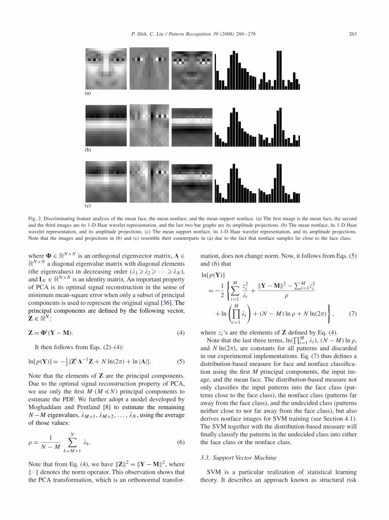
The vectors X, Xh, Xv , Xr , and Xc are normalized to zeromean and unit variance, respectively. The normalized vectorsare then concatenated to form a new feature vector Y ∈ RN ,where N = 3mn. Finally, the feature vector Y is normalizedto zero mean and unit variance to form the discriminatingfeature vector for face detection. Fig. 2(a) shows the meanface (i.e., the average of the training face images), its 1-DHaar wavelet representation, and its amplitude projections.The first image is the mean face. The second and the thirdimages are the vertical and the horizontal difference imagesof the mean face, respectively, which correspond to the 1-DHaar wavelet representation. The last two bar graphs drawthe vertical (column) and horizontal (row) projections of themean face, which correspond to the amplitude projections.Fig. 2(b) shows the mean nonface (i.e., the average of thetraining nonface images), its 1-D Haar wavelet representa-tion, and its amplitude projections. Fig. 2(c) shows the meansupport nonface (i.e., the average of the support nonface im-ages, which are chosen from the training nonface images bySVM, see Section 3.3), its 1-D Haar wavelet representation,and its amplitude projections. Note that the images and pro-jections in Fig. 2(b) and (c) resemble their counterparts inFig. 2(a) due to the fact that the nonface samples lie close tothe face class. Furthermore, Fig. 2(c) looks more like a facethan Fig. 2(b) does because Fig. 2(c) is the mean of sup-port nonfaces, which lie closer to the face class than othernonfaces do.

3.2. Face class modeling and distribution-based measure

Statistical modeling of the face class defines in essencethe PDF, of the face class. A common assumption of thePDF is a multivariate normal distribution, which is especiallyreasonable if one models only the upright frontal faces thatare properly aligned to one another [8,28]. Note that thetraining face images are all upright, frontal, and properlyaligned, the density function of the face class is, therefore,modeled as a multivariate normal distribution

p(Y) = 1

(2�)N/2|�|1/2

× exp

{−1

2(Y − M)t�−1(Y − M)

}, (1)

where Y ∈ RN is the discriminating feature vector, M ∈RN and � ∈ RN×N are the mean vector and the covariancematrix of the face class, �f , respectively. Take the naturallogarithm on both sides, we have

ln[p(Y)] = − 12 {(Y − M)t�−1(Y − M)

+ N ln(2�) + ln |�|}. (2)

The covariance matrix, �, can be factorized into the fol-lowing form using PCA [35]:

� = ��t with ��t = �t� = IN ,

� = diag{�1, �2, . . . , �N }, (3)


Fig. 2. Discriminating feature analysis of the mean face, the mean nonface, and the mean support nonface. (a) The first image is the mean face, the secondand the third images are its 1-D Haar wavelet representation, and the last two bar graphs are its amplitude projections. (b) The mean nonface, its 1-D Haarwavelet representation, and its amplitude projections. (c) The mean support nonface, its 1-D Haar wavelet representation, and its amplitude projections.Note that the images and projections in (b) and (c) resemble their counterparts in (a) due to the fact that nonface samples lie close to the face class.

where � ∈ RN×N is an orthogonal eigenvector matrix, � ∈RN×N a diagonal eigenvalue matrix with diagonal elements(the eigenvalues) in decreasing order (�1 ��2 � · · · ��N ),and IN ∈ RN×N is an identity matrix. An important propertyof PCA is its optimal signal reconstruction in the sense ofminimum mean-square error when only a subset of principalcomponents is used to represent the original signal [36]. Theprincipal components are defined by the following vector,Z ∈ RN :

Z = �t(Y − M). (4)

It then follows from Eqs. (2)–(4):

ln[p(Y)] = − 12 {Zt�−1Z + N ln(2�) + ln |�|}. (5)

Note that the elements of Z are the principal components.Due to the optimal signal reconstruction property of PCA,we use only the first M (M>N ) principal components toestimate the PDF. We further adopt a model developed byMoghaddam and Pentland [8] to estimate the remainingN−M eigenvalues, �M+1, �M+2, . . . , �N , using the averageof those values:

� = 1

N − M

N∑k=M+1

�k . (6)

Note that from Eq. (4), we have ‖Z‖2 = ‖Y − M‖2, where‖ · ‖ denotes the norm operator. This observation shows thatthe PCA transformation, which is an orthonormal transfor-

mation, does not change norm. Now, it follows from Eqs. (5)and (6) that

ln[p(Y)]

= −1

2

{M∑i=1

z2i

�i

+ ‖Y − M‖2 −∑Mi=1z

2i

�

+ ln

(M∏i=1

�i

)+ (N − M) ln � + N ln(2�)

}, (7)

where zi’s are the elements of Z defined by Eq. (4).Note that the last three terms, ln(

∏Mi=1 �i ), (N −M) ln �,

and N ln(2�), are constants for all patterns and discardedin our experimental implementations. Eq. (7) thus defines adistribution-based measure for face and nonface classifica-tion using the first M principal components, the input im-age, and the mean face. The distribution-based measure notonly classifies the input patterns into the face class (pat-terns close to the face class), the nonface class (patterns faraway from the face class), and the undecided class (patternsneither close to nor far away from the face class), but alsoderives nonface images for SVM training (see Section 4.1).The SVM together with the distribution-based measure willfinally classify the patterns in the undecided class into eitherthe face class or the nonface class.

3.3. Support Vector Machine

SVM is a particular realization of statistical learningtheory. It describes an approach known as structural risk


minimization, which minimizes the risk functional in termsof both the empirical risk and the confidence interval [29].The main idea of SVM comes from (i) a nonlinear map-ping of the input space to a high-dimensional feature space,and (ii) designing the optimal hyperplane in terms of themaximal margin between the patterns of the two classes inthe feature space. SVM, which displays good generaliza-tion performance, has been applied extensively for patternclassification, regression, and density estimation.

Let (x1, y1), (x2, y2), . . . , (xk, yk), xi ∈ RN , and yi ∈{+1, −1} be k training samples in the input space, where yi

indicates the class membership of xi . Let � be a nonlinearmapping between the input space and the feature space, � :RN → F, i.e., x → �(x). The optimal hyperplane in thefeature space is defined as follow:

w0 · �(x) + b0 = 0. (8)

It can be proven [29] that the weight vector w0 is a linearcombination of the support vectors, which are the vectors xi

that satisfy yi(w0 · �(xi ) + b0) = 1:

w0 =∑

support vectors

yi�i�(xi ), (9)

where �i’s are determined by maximizing the followingfunctional:

L(�) =k∑

i=1

�i − 1

2

k∑i,j=1

�i�j yiyj�(xi ) · �(xj ) (10)

subject to the following constraints:

k∑i=1

�iyi = 0, �i �0, i = 1, 2, . . . , k. (11)

From Eqs. (8) and (9), we can derive the linear decisionfunction in the feature space

f (x) = sign

⎛⎝ ∑

support vectors

yi�i�(xi ) · �(x) + b0

⎞⎠ . (12)

Note that the decision function (seeEq. (12)) is defined by the dot products in the high-dimensional feature space, where computation might beprohibitively expensive. SVM, however, manages to com-pute the dot products by means of a kernel function [29]

K(xi , xj ) = �(xi ) · �(xj ). (13)

Three classes of kernel functions widely used in kernel clas-sifiers, neural networks, and SVMs are polynomial kernels,Gaussian kernels, and sigmoid kernels [29]:

K(xi , xj ) = (xi · xj )d , (14)

K(xi , xj ) = exp

(−‖xi − xj‖2

2�2

), (15)

K(xi , xj ) = tanh(�(xi · xj ) + ϑ), (16)

where d ∈ N, � > 0, � > 0, and ϑ < 0.

3.4. Face detection using distribution-based measure andSVM

The first decision rule applies the distribution-based mea-sure (Eq. (7)) to detect faces that are very close to the faceclass and exclude patterns that are very far away from theface class. This decision rule separates the patterns in theinput image into three classes: the face class (�f ), the non-face class (�n), and the undecided class (�u):

Y ∈{�f if ln[p(Y)]�f ,

�u if n < ln[p(Y)] < f ,

�n otherwise,(17)

where Y is the discriminating feature vector derived froman input pattern, ln[p(Y)] is the distribution-based measuredefined by Eq. (7), and f and n are thresholds.

The second decision rule, the SVM decision rule, thenapplies the SVM classifier to detect faces in the �u class:

Y ∈{

�f if f (Y) > 0,

�n otherwise,(18)

where f (Y) is the decision function of the SVM classifierdefined by Eq. (12). Our experiments, however, show thatthe SVM classifier alone cannot detect all the faces in the�u class, and some face patterns are misclassified to the �n

class.To improve the face detection performance of our method,

we design the third decision rule, the DFA–SVM decisionrule, which further checks the patterns assigned to the �n

class from the �u class:

Y ∈{

�f if g(Y) > s and ln[p(Y)] + cg(Y) > t ,

�n otherwise,(19)

where c is a positive constant, s and t are thresholds, andg(Y) is the decision value of the SVM classifier without thesign function (see Eq. (12)):

g(Y) =∑

support vectors

yi�i�(xi ) · �(Y) + b0. (20)

Note that the functionality of the first term, g(Y) > s , isto select candidate face patterns misclassified to the �n

class by the SVM classifier (see Eq. (18)); the second term,ln[p(Y)]+cg(Y) > t , then further determines the true facesfrom the candidate patterns by linearly combining the de-cision values from the distribution-based measure and theSVM classifier.

The three decision rules detailed above actually apply acoarse-to-fine classification strategy in the sense that they


are cascaded in an increasing order of detection accuracyand decreasing order of computational efficiency. Regardingdetection accuracy, the third decision rule detects faces moreaccurately than the first two rules do because it combines theclassification power of the distribution-based measure andSVM. As to computational efficiency, the first decision ruleruns faster than the second and the third one due to the factthat the term ln[p(Y)] is evaluated by estimating the first Mprincipal components of the input vector Y, while the termg(Y) is obtained directly in the original input space, RN .Note that M is much smaller than N (see Section 3.2).

4. Experiments

This section details statistical learning, learning thethresholds, face detection performance, and computationalcomplexity of the DFA–SVM method. The training data forthe DFA–SVM method comes from the FERET database[9] Batch 15, which contains 600 frontal face images. Thetesting data comes from the MIT–CMU test sets [10], whichinclude images from diverse sources. Experimental results

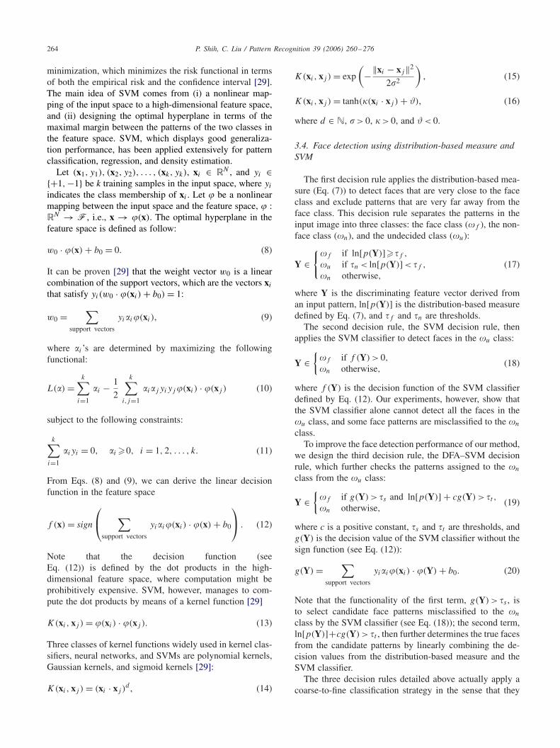
Fig. 3. Some examples of the face and the nonface training images: (a) examples of the face training images; (b) examples of the nonface training images.

show that our DFA–SVM method, which is trained on asimple image set yet works on much more complex images,displays robust generalization performance.

4.1. Statistical learning of the DFA–SVM method

The statistical learning of the DFA–SVM method includesthree stages: face class modeling, nonface image generation,and SVM. First, the DFA–SVM method models the faceclass, �f , as a multivariate normal distribution and defines adistribution-based measure, ln[p(Y)], using 600 frontal faceimages from the FERET database Batch 15 [9]. Note thatwe also include the mirror images of the training data; hencethe total training images for face class modeling is 1200.

Second, nonface training images are derived by choosingsubimages from 14 natural scene images that do not containany face at all. The subimages that lie close to (in the senseof the distribution-based measure, ln[p(Y)]) the face classare chosen as nonface training images:

ln[p(Y)] > n, (21)


-0.85 -0.8 -0.75 -0.7 -0.65 -0.6 -0.55 -0.5 -0.450

500

1000

1500

2000

2500

3000

3500

4000

4500

Tot

al N

umbe

r of

Non

face

Sub

imag

es

�n�u

τnτf τf

ω f

∗

NonfaceSamples

FaceSamples

ln[p(Y)]

τn

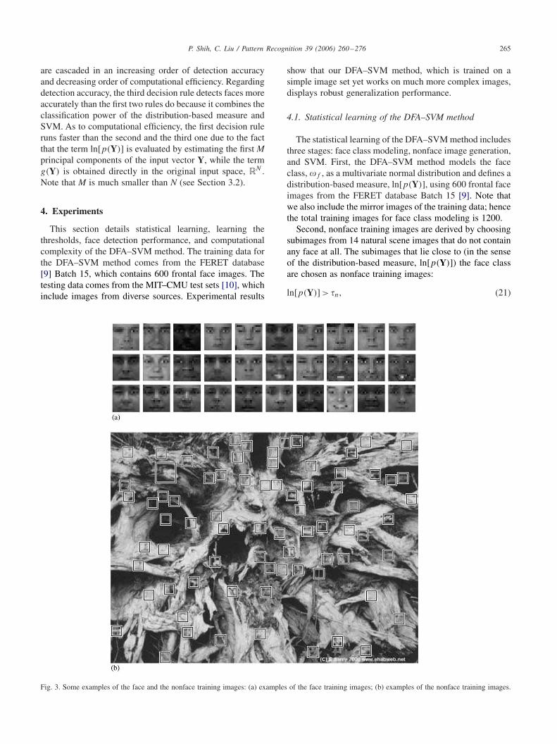
Fig. 4. The learning of thresholds n and f . (a) The relationship between the total number of nonface subimages and the threshold n. The horizontalaxis indicates the value of n and the vertical axis is the total number of nonface subimages derived from all the 14 natural scene images used in ourexperiments. (b) The threshold, f , is set to be the largest distribution-based measure of all these nonface images. Note that in our experiments, thethreshold f is increased to ∗

fto reduce the number of false detections.

where ln[p(Y)] is the distribution-based measure (seeEq. (7)) and n is the threshold (see Eq. (17)). Note that thenumber of principal components, M, defined in Eq. (7) isfixed at 10 throughout our experiments.

Finally, we apply the 1200 face images and 3813 non-face images to train a SVM with a polynomial kernel ofdegree 2 for face detection. Note that both the face andthe nonface images are normalized to a spatial resolutionof 16 × 16. Fig. 3(a) shows some examples of the facetraining images that are normalized to 16 × 16, and Fig.3(b) shows some examples of the nonface training im-ages derived from a natural scene image. Note that thenonface images in Fig. 3(b) display different sizes, whichcorrespond to different scales of the original natural sceneimage when the nonface images are derived. The spatialresolution of all the nonface images, however, is the same,16 × 16.

4.2. Learning the thresholds

Thresholds play important roles in our DFA–SVM facedetection method as a change of a threshold may affect thesystem performance significantly. This section describes ageneral procedure to fine-tune the four thresholds, n, f ,s , and t , defined in Section 3.4.

4.2.1. Thresholds f and n

The learning of thresholds starts with n as it directlydetermines the number of nonface training images derivedfrom the 14 natural scene images (see Eq. (21)). Fig. 4(a)plots the relationship between the total number of nonfaceimages and the threshold n. The horizontal axis indicatesthe value of n, and the vertical axis is the total number ofnonface images derived from all the 14 natural scene images.Note that in order to prevent one scene image from unduly


-1.48-1.08

-0.68-0.28

0.12

-0.7-0.68-0.66-0.64-0.62

10

20

30

40

Num

ber

of M

isse

d F

aces

-1.48-1.08-0.68-0.280.12

-0.7-0.68

-0.66-0.64

-0.62

10

20

30

40

Num

ber

of F

alse

Det

ectio

ns

(a)

-1.48-1.08

-0.68-0.28

0.12

-0.7-0.68-0.66-0.64-0.62

10

20

30

40

Num

ber

of T

otal

Err

ors

τ s

τ s

τ s

τ t

τ t

τ t

(a) (b)

(c)

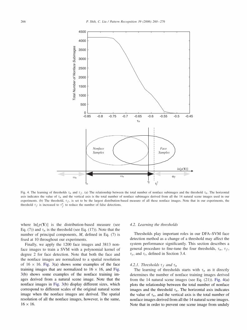
Fig. 5. The learning of thresholds s and t : (a) the number of missed faces increases when either s or t increases; (b) the number of false detectionsdecreases when either s or t increases; (c) the number of total errors (missed faces + false detections) versus the thresholds s and t . The smallesttotal error occurs at {−0.68, −0.66}.

dominating the others, we cap the number of nonface imagesfor each scene at 300. As a result, the maximum number ofnonface images derived from all the scene images should be4200, which is shown in Fig. 4(a) by the flat curve segment.Our choice of n is thus close to the threshold value that leadsto this flat curve segment. In particular, the chosen thresh-old n generates 3813 nonface images from the 14 naturalscene images, and these generated images form the nonfacetraining set for the DFA–SVM face detection method.

After generating the nonface images, a reasonable choiceof the threshold, f , is the largest distribution-based measureof all these nonface images (see Fig. 4(b)). However, Eq. (17)is applied for coarse detection, whose purpose is to reliablyclassify face and nonface patterns while leaving difficultpatterns in the undecided class. We therefore increase thethreshold from f to ∗

f (see Fig. 4(b)) to reduce the numberof false detections.

4.2.2. Thresholds s and t

The thresholds, s and t , in Eq. (19) are used for the finedetection, whose functionality is to classify the undecidedpatterns into either the face class or the nonface class. The

values of these two thresholds are determined through anumerical analysis procedure. Let s be a set of values ofs and t be a set of values of t , we evaluated the facedetection performance of each combination of s ×t usinga subset (24 images containing 54 faces) of the MIT–CMUtest sets. Note that the parameter, c, defined in Eq. (19) isfixed at 0.05 throughout our experiments.

Figs. 5(a), (b), and (c) show the number of missed facesversus the thresholds (s and t ), the number of false detec-tions versus the thresholds, and the number of total errors(missed faces + false detections) versus the thresholds, re-spectively. Fig. 5(a) shows that the number of missed faceincreases when either s or t increases. Fig. 5(b) shows,however, that the number of false detections decreases wheneither s or t increases. Finally, Fig. 5(c) shows that thesmallest total error occurs at {−0.68, −0.66}. We thereforeset s and t to be −0.68 and −0.66, respectively.

4.3. Face detection performance of the DFA–SVM method

The data used to test our DFA–SVM method forface detection comes from the MIT–CMU test sets [10].


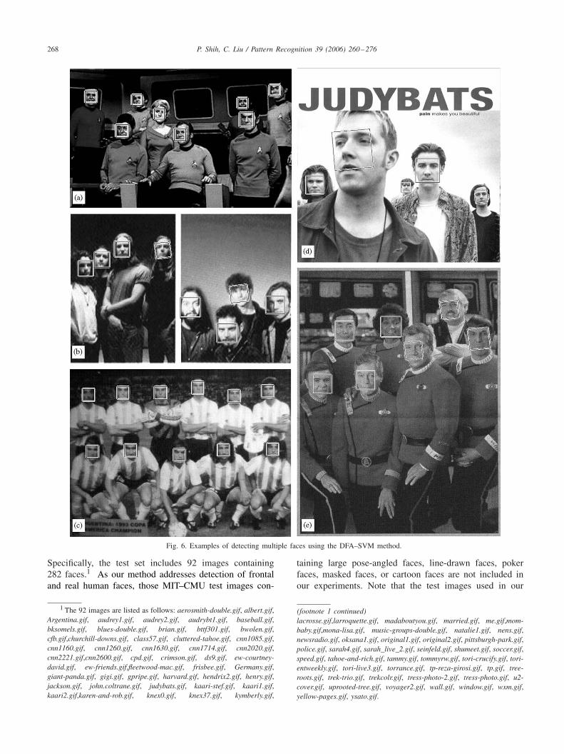
Fig. 6. Examples of detecting multiple faces using the DFA–SVM method.

Specifically, the test set includes 92 images containing282 faces.1 As our method addresses detection of frontaland real human faces, those MIT–CMU test images con-

1 The 92 images are listed as follows: aerosmith-double.gif, albert.gif,Argentina.gif, audrey1.gif, audrey2.gif, audrybt1.gif, baseball.gif,bksomels.gif, blues-double.gif, brian.gif, bttf301.gif, bwolen.gif,cfb.gif,churchill-downs.gif, class57.gif, cluttered-tahoe.gif, cnn1085.gif,cnn1160.gif, cnn1260.gif, cnn1630.gif, cnn1714.gif, cnn2020.gif,cnn2221.gif,cnn2600.gif, cpd.gif, crimson.gif, ds9.gif, ew-courtney-david.gif, ew-friends.gif,fleetwood-mac.gif, frisbee.gif, Germany.gif,giant-panda.gif, gigi.gif, gpripe.gif, harvard.gif, hendrix2.gif, henry.gif,jackson.gif, john.coltrane.gif, judybats.gif, kaari-stef.gif, kaari1.gif,kaari2.gif,karen-and-rob.gif, knex0.gif, knex37.gif, kymberly.gif,

taining large pose-angled faces, line-drawn faces, pokerfaces, masked faces, or cartoon faces are not included inour experiments. Note that the test images used in our

(footnote 1 continued)lacrosse.gif,larroquette.gif, madaboutyou.gif, married.gif, me.gif,mom-baby.gif,mona-lisa.gif, music-groups-double.gif, natalie1.gif, nens.gif,newsradio.gif, oksana1.gif, original1.gif, original2.gif, pittsburgh-park.gif,police.gif, sarah4.gif, sarah_live_2.gif, seinfeld.gif, shumeet.gif, soccer.gif,speed.gif, tahoe-and-rich.gif, tammy.gif, tommyrw.gif, tori-crucify.gif, tori-entweekly.gif, tori-live3.gif, torrance.gif, tp-reza-girosi.gif, tp.gif, tree-roots.gif, trek-trio.gif, trekcolr.gif, tress-photo-2.gif, tress-photo.gif, u2-cover.gif, uprooted-tree.gif, voyager2.gif, wall.gif, window.gif, wxm.gif,yellow-pages.gif, ysato.gif.


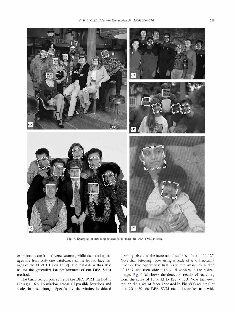
Fig. 7. Examples of detecting rotated faces using the DFA–SVM method.

experiments are from diverse sources, while the training im-ages are from only one database, i.e., the frontal face im-ages of the FERET Batch 15 [9]. The test data is thus ableto test the generalization performance of our DFA–SVMmethod.

The basic search procedure of the DFA–SVM method issliding a 16 × 16 window across all possible locations andscales in a test image. Specifically, the window is shifted

pixel-by-pixel and the incremental scale is a factor of 1.125.Note that detecting faces using a scale of k × k actuallyinvolves two operations: first resize the image by a ratioof 16/k, and then slide a 16 × 16 window in the resizedimage. Fig. 6 (a) shows the detection results of searchingfrom the scale of 12 × 12 to 120 × 120. Note that eventhough the sizes of faces appeared in Fig. 6(a) are smallerthan 20 × 20, the DFA–SVM method searches at a wide


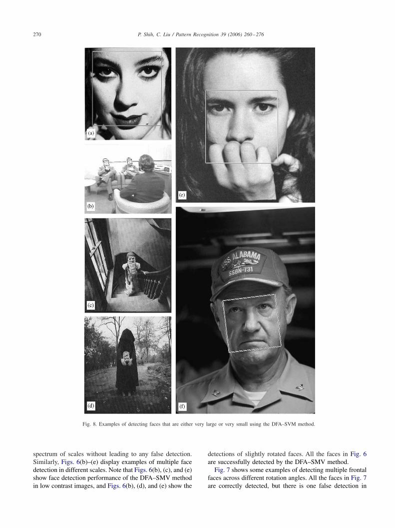
Fig. 8. Examples of detecting faces that are either very large or very small using the DFA–SVM method.

spectrum of scales without leading to any false detection.Similarly, Figs. 6(b)–(e) display examples of multiple facedetection in different scales. Note that Figs. 6(b), (c), and (e)show face detection performance of the DFA–SMV methodin low contrast images, and Figs. 6(b), (d), and (e) show the

detections of slightly rotated faces. All the faces in Fig. 6are successfully detected by the DFA–SMV method.

Fig. 7 shows some examples of detecting multiple frontalfaces across different rotation angles. All the faces in Fig. 7are correctly detected, but there is one false detection in


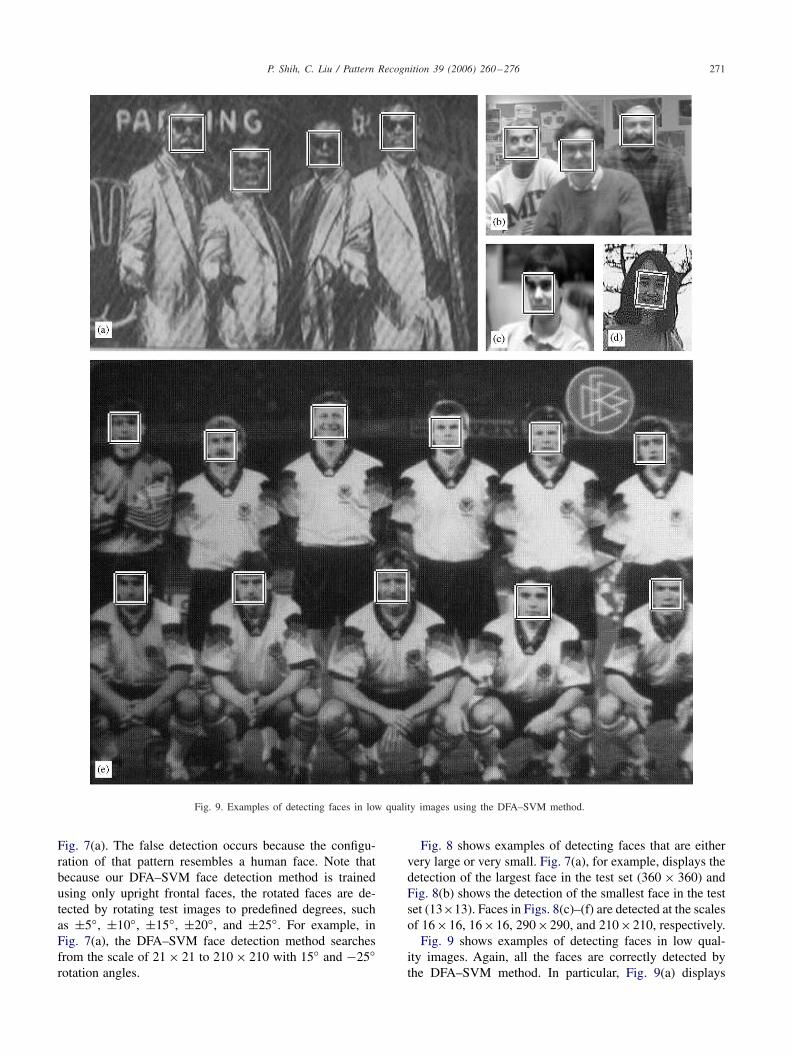
Fig. 9. Examples of detecting faces in low quality images using the DFA–SVM method.

Fig. 7(a). The false detection occurs because the configu-ration of that pattern resembles a human face. Note thatbecause our DFA–SVM face detection method is trainedusing only upright frontal faces, the rotated faces are de-tected by rotating test images to predefined degrees, suchas ±5◦, ±10◦, ±15◦, ±20◦, and ±25◦. For example, inFig. 7(a), the DFA–SVM face detection method searchesfrom the scale of 21 × 21 to 210 × 210 with 15◦ and −25◦rotation angles.

Fig. 8 shows examples of detecting faces that are eithervery large or very small. Fig. 7(a), for example, displays thedetection of the largest face in the test set (360 × 360) andFig. 8(b) shows the detection of the smallest face in the testset (13×13). Faces in Figs. 8(c)–(f) are detected at the scalesof 16×16, 16×16, 290×290, and 210×210, respectively.

Fig. 9 shows examples of detecting faces in low qual-ity images. Again, all the faces are correctly detected bythe DFA–SVM method. In particular, Fig. 9(a) displays


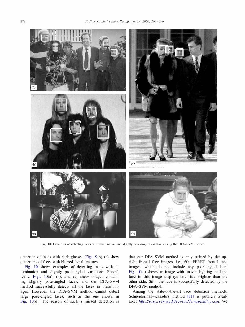
Fig. 10. Examples of detecting faces with illumination and slightly pose-angled variations using the DFA–SVM method.

detection of faces with dark glasses; Figs. 9(b)–(e) showdetections of faces with blurred facial features.

Fig. 10 shows examples of detecting faces with il-lumination and slightly pose-angled variations. Specif-ically, Figs. 10(a), (b), and (e) show images contain-ing slightly pose-angled faces, and our DFA–SVMmethod successfully detects all the faces in these im-ages. However, the DFA–SVM method cannot detectlarge pose-angled faces, such as the one shown inFig. 10(d). The reason of such a missed detection is

that our DFA–SVM method is only trained by the up-right frontal face images, i.e., 600 FERET frontal faceimages, which do not include any pose-angled face.Fig. 10(c) shows an image with uneven lighting, and theface in this image displays one side brighter than theother side. Still, the face is successfully detected by theDFA–SVM method.

Among the state-of-the-art face detection methods,Schneiderman–Kanade’s method [11] is publicly avail-able: http://vasc.ri.cmu.edu/cgi-bin/demos/findface.cgi. We

http://vasc.ri.cmu.edu/cgi-bin/demos/findface.cgi


therefore compare our DFA–SVM face detection methodwith Schneiderman–Kanade’s method [11]. This methodhas two thresholds, the frontal detection threshold andthe profile detection threshold, which control the num-ber of faces detected and the number of false detections.Table 1 shows the comparative face detection performanceof Schneiderman–Kanade’s method and our DFA–SVMmethod. Note that the two numbers in the parenthesescorrespond to the frontal detection threshold and the pro-file detection threshold, respectively. Experimental resultsshow that Schneiderman–Kanade’s method achieves 96.1%face detection accuracy with 41 false detections when thethresholds are set to be 1.0. Note that the number of falsedetections of Schneiderman–Kanade’s method counted hereonly refers to the frontal face false detections, and it doesnot include the false detections caused by profile face de-tection. The face detection rate of Schneiderman–Kanade’smethod decreases when the thresholds get larger. OurDFA–SVM method, achieving 98.2% face detection accu-racy, thus compares favorably against the state-of-the-artface detection methods, such as Schneiderman–Kanade’smethod [11].

4.4. Computational efficiency

We apply two criteria to improve the computational effi-ciency of the DFA–SVM method: the single response crite-rion and the early exclusion criterion. The single responsecriterion avoids multiple responses to a singe face, whilethe early exclusion criterion applies heuristic procedures toexclude subimages that cannot be face.

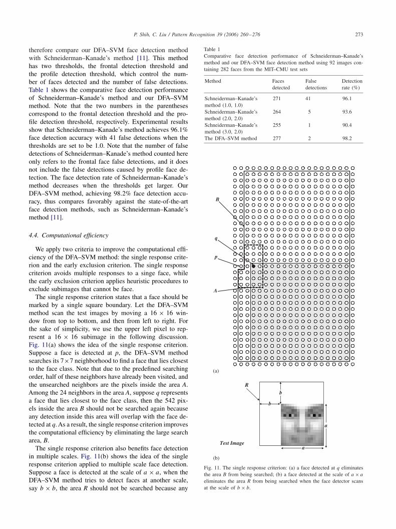
The single response criterion states that a face should bemarked by a single square boundary. Let the DFA–SVMmethod scan the test images by moving a 16 × 16 win-dow from top to bottom, and then from left to right. Forthe sake of simplicity, we use the upper left pixel to rep-resent a 16 × 16 subimage in the following discussion.Fig. 11(a) shows the idea of the single response criterion.Suppose a face is detected at p, the DFA–SVM methodsearches its 7×7 neighborhood to find a face that lies closestto the face class. Note that due to the predefined searchingorder, half of these neighbors have already been visited, andthe unsearched neighbors are the pixels inside the area A.Among the 24 neighbors in the area A, suppose q representsa face that lies closest to the face class, then the 542 pix-els inside the area B should not be searched again becauseany detection inside this area will overlap with the face de-tected at q. As a result, the single response criterion improvesthe computational efficiency by eliminating the large searcharea, B.

The single response criterion also benefits face detectionin multiple scales. Fig. 11(b) shows the idea of the singleresponse criterion applied to multiple scale face detection.Suppose a face is detected at the scale of a × a, when theDFA–SVM method tries to detect faces at another scale,say b × b, the area R should not be searched because any

Table 1Comparative face detection performance of Schneiderman–Kanade’smethod and our DFA–SVM face detection method using 92 images con-taining 282 faces from the MIT–CMU test sets

Method Faces False Detectiondetected detections rate (%)

Schneiderman–Kanade’s 271 41 96.1method (1.0, 1.0)Schneiderman–Kanade’s 264 5 93.6method (2.0, 2.0)Schneiderman–Kanade’s 255 1 90.4method (3.0, 2.0)The DFA–SVM method 277 2 98.2

B

q

p

A

(a)

a

b

b

a

R

Test Image

(b)

Fig. 11. The single response criterion: (a) a face detected at q eliminatesthe area B from being searched; (b) a face detected at the scale of a × a

eliminates the area R from being searched when the face detector scansat the scale of b × b.


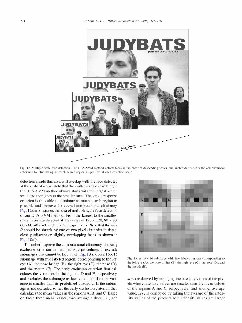
Fig. 12. Multiple scale face detection. The DFA–SVM method detects faces in the order of descending scales, and such order benefits the computationalefficiency by eliminating as much search region as possible at each detection scale.

detection inside this area will overlap with the face detectedat the scale of a×a. Note that the multiple scale searching inthe DFA–SVM method always starts with the largest searchscale and then goes to the smaller ones. The single responsecriterion is thus able to eliminate as much search region aspossible and improve the overall computational efficiency.Fig. 12 demonstrates the idea of multiple scale face detectionof our DFA–SVM method. From the largest to the smallestscale, faces are detected at the scales of 120 ×120, 80 ×80,60×60, 40×40, and 30×30, respectively. Note that the areaR should be shrunk by one or two pixels in order to detectclosely adjacent or slightly overlapping faces as shown inFig. 10(d).

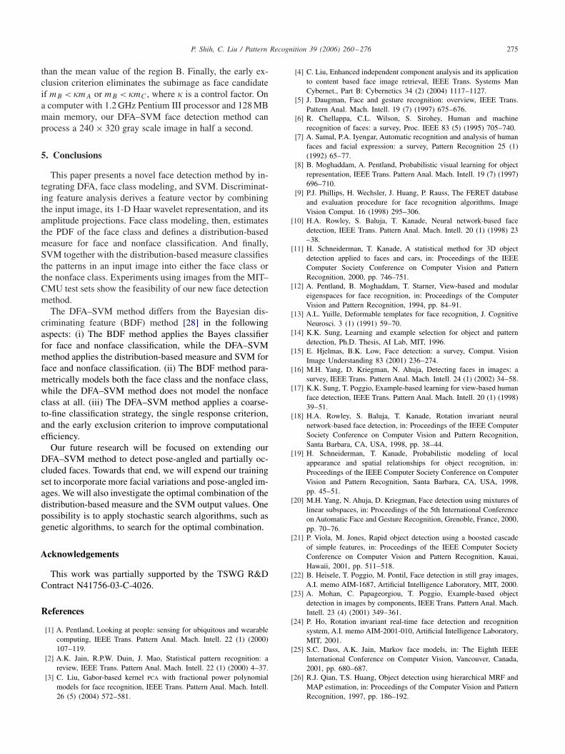
To further improve the computational efficiency, the earlyexclusion criterion defines heuristic procedures to excludesubimages that cannot be face at all. Fig. 13 shows a 16×16subimage with five labeled regions corresponding to the lefteye (A), the nose bridge (B), the right eye (C), the nose (D),and the mouth (E). The early exclusion criterion first cal-culates the variances in the regions D and E, respectively,and excludes the subimage as face candidate if either vari-ance is smaller than its predefined threshold. If the subim-age is not excluded so far, the early exclusion criterion thencalculates the mean values in the regions A, B, and C. Basedon these three mean values, two average values, mA and

D

E

A B C

Fig. 13. A 16 × 16 subimage with five labeled regions corresponding tothe left eye (A), the nose bridge (B), the right eye (C), the nose (D), andthe mouth (E).

mC , are derived by averaging the intensity values of the pix-els whose intensity values are smaller than the mean valuesof the regions A and C, respectively; and another averagevalue, mB , is computed by taking the average of the inten-sity values of the pixels whose intensity values are larger


than the mean value of the region B. Finally, the early ex-clusion criterion eliminates the subimage as face candidateif mB < �mA or mB < �mC , where � is a control factor. Ona computer with 1.2 GHz Pentium III processor and 128 MBmain memory, our DFA–SVM face detection method canprocess a 240 × 320 gray scale image in half a second.

5. Conclusions

This paper presents a novel face detection method by in-tegrating DFA, face class modeling, and SVM. Discriminat-ing feature analysis derives a feature vector by combiningthe input image, its 1-D Haar wavelet representation, and itsamplitude projections. Face class modeling, then, estimatesthe PDF of the face class and defines a distribution-basedmeasure for face and nonface classification. And finally,SVM together with the distribution-based measure classifiesthe patterns in an input image into either the face class orthe nonface class. Experiments using images from the MIT–CMU test sets show the feasibility of our new face detectionmethod.

The DFA–SVM method differs from the Bayesian dis-criminating feature (BDF) method [28] in the followingaspects: (i) The BDF method applies the Bayes classifierfor face and nonface classification, while the DFA–SVMmethod applies the distribution-based measure and SVM forface and nonface classification. (ii) The BDF method para-metrically models both the face class and the nonface class,while the DFA–SVM method does not model the nonfaceclass at all. (iii) The DFA–SVM method applies a coarse-to-fine classification strategy, the single response criterion,and the early exclusion criterion to improve computationalefficiency.

Our future research will be focused on extending ourDFA–SVM method to detect pose-angled and partially oc-cluded faces. Towards that end, we will expend our trainingset to incorporate more facial variations and pose-angled im-ages. We will also investigate the optimal combination of thedistribution-based measure and the SVM output values. Onepossibility is to apply stochastic search algorithms, such asgenetic algorithms, to search for the optimal combination.

Acknowledgements

This work was partially supported by the TSWG R&DContract N41756-03-C-4026.

References

[1] A. Pentland, Looking at people: sensing for ubiquitous and wearablecomputing, IEEE Trans. Pattern Anal. Mach. Intell. 22 (1) (2000)107–119.

[2] A.K. Jain, R.P.W. Duin, J. Mao, Statistical pattern recognition: areview, IEEE Trans. Pattern Anal. Mach. Intell. 22 (1) (2000) 4–37.

[3] C. Liu, Gabor-based kernel PCA with fractional power polynomialmodels for face recognition, IEEE Trans. Pattern Anal. Mach. Intell.26 (5) (2004) 572–581.

[4] C. Liu, Enhanced independent component analysis and its applicationto content based face image retrieval, IEEE Trans. Systems ManCybernet., Part B: Cybernetics 34 (2) (2004) 1117–1127.

[5] J. Daugman, Face and gesture recognition: overview, IEEE Trans.Pattern Anal. Mach. Intell. 19 (7) (1997) 675–676.

[6] R. Chellappa, C.L. Wilson, S. Sirohey, Human and machinerecognition of faces: a survey, Proc. IEEE 83 (5) (1995) 705–740.

[7] A. Samal, P.A. Iyengar, Automatic recognition and analysis of humanfaces and facial expression: a survey, Pattern Recognition 25 (1)(1992) 65–77.

[8] B. Moghaddam, A. Pentland, Probabilistic visual learning for objectrepresentation, IEEE Trans. Pattern Anal. Mach. Intell. 19 (7) (1997)696–710.

[9] P.J. Phillips, H. Wechsler, J. Huang, P. Rauss, The FERET databaseand evaluation procedure for face recognition algorithms, ImageVision Comput. 16 (1998) 295–306.

[10] H.A. Rowley, S. Baluja, T. Kanade, Neural network-based facedetection, IEEE Trans. Pattern Anal. Mach. Intell. 20 (1) (1998) 23–38.

[11] H. Schneiderman, T. Kanade, A statistical method for 3D objectdetection applied to faces and cars, in: Proceedings of the IEEEComputer Society Conference on Computer Vision and PatternRecognition, 2000, pp. 746–751.

[12] A. Pentland, B. Moghaddam, T. Starner, View-based and modulareigenspaces for face recognition, in: Proceedings of the ComputerVision and Pattern Recognition, 1994, pp. 84–91.

[13] A.L. Yuille, Deformable templates for face recognition, J. CognitiveNeurosci. 3 (1) (1991) 59–70.

[14] K.K. Sung, Learning and example selection for object and patterndetection, Ph.D. Thesis, AI Lab, MIT, 1996.

[15] E. Hjelmas, B.K. Low, Face detection: a survey, Comput. VisionImage Understanding 83 (2001) 236–274.

[16] M.H. Yang, D. Kriegman, N. Ahuja, Detecting faces in images: asurvey, IEEE Trans. Pattern Anal. Mach. Intell. 24 (1) (2002) 34–58.

[17] K.K. Sung, T. Poggio, Example-based learning for view-based humanface detection, IEEE Trans. Pattern Anal. Mach. Intell. 20 (1) (1998)39–51.

[18] H.A. Rowley, S. Baluja, T. Kanade, Rotation invariant neuralnetwork-based face detection, in: Proceedings of the IEEE ComputerSociety Conference on Computer Vision and Pattern Recognition,Santa Barbara, CA, USA, 1998, pp. 38–44.

[19] H. Schneiderman, T. Kanade, Probabilistic modeling of localappearance and spatial relationships for object recognition, in:Proceedings of the IEEE Computer Society Conference on ComputerVision and Pattern Recognition, Santa Barbara, CA, USA, 1998,pp. 45–51.

[20] M.H. Yang, N. Ahuja, D. Kriegman, Face detection using mixtures oflinear subspaces, in: Proceedings of the 5th International Conferenceon Automatic Face and Gesture Recognition, Grenoble, France, 2000,pp. 70–76.

[21] P. Viola, M. Jones, Rapid object detection using a boosted cascadeof simple features, in: Proceedings of the IEEE Computer SocietyConference on Computer Vision and Pattern Recognition, Kauai,Hawaii, 2001, pp. 511–518.

[22] B. Heisele, T. Poggio, M. Pontil, Face detection in still gray images,A.I. memo AIM-1687, Artificial Intelligence Laboratory, MIT, 2000.

[23] A. Mohan, C. Papageorgiou, T. Poggio, Example-based objectdetection in images by components, IEEE Trans. Pattern Anal. Mach.Intell. 23 (4) (2001) 349–361.

[24] P. Ho, Rotation invariant real-time face detection and recognitionsystem, A.I. memo AIM-2001-010, Artificial Intelligence Laboratory,MIT, 2001.

[25] S.C. Dass, A.K. Jain, Markov face models, in: The Eighth IEEEInternational Conference on Computer Vision, Vancouver, Canada,2001, pp. 680–687.

[26] R.J. Qian, T.S. Huang, Object detection using hierarchical MRF andMAP estimation, in: Proceedings of the Computer Vision and PatternRecognition, 1997, pp. 186–192.


[27] R. Hsu, M. Abdel-Mottaleb, A. Jain, Face detection in color images,IEEE Trans. Pattern Anal. Mach. Intell. 24 (5) (2002) 696–706.

[28] C. Liu, A Bayesian discriminating features method for face detection,IEEE Trans. Pattern Anal. Mach. Intell. 25 (6) (2003) 725–740.

[29] Y.N. Vapnik, The Nature of Statistical Learning Theory, second ed.,Springer, Berlin, 1999.

[30] E. Osuna, R. Freund, F. Girosi, Training support vector machines:an application to face detection, in: Proceedings of the ComputerVision and Pattern Recognition, Puerto Rico, 1997.

[31] C.P. Papageorgiou, M. Oren, T. Poggio, A general framework forobject detection, in: Proceedings of the International Conference onComputer Vision, Bombay, India, 1998, pp. 555–562.

[32] S. Romdhani, P. Torr, B. Schölkopf, A. Blake, Computationallyefficient face detection, in: The Eighth IEEE International Conferenceon Computer Vision, Vancouver, Canada, 2001.

[33] M.S. Bartlett, G. Littlewort, I. Fasel, J.R. Movellan, Real timeface detection and facial expression recognition: development andapplications to human computer interaction, in: Proceedings of theComputer Vision and Pattern Recognition, Madison, Wisconsin, 2003.

[34] B. Heisele, T. Serre, S. Prentice, T. Poggio, Hierarchicalclassification and feature reduction for fast face detection withsupport vector machines, Pattern Recognition 36 (9) (2003)2007–2017.

[35] C. Liu, H. Wechsler, Robust coding schemes for indexing and retrievalfrom large face databases, IEEE Trans. Image Process. 9 (1) (2000)132–137.

[36] C. Liu, H. Wechsler, Gabor feature based classification using theenhanced Fisher linear discriminant model for face recognition, IEEETrans. Image Process. 11 (4) (2002) 467–476.

About the Author—PEICHUNG SHIH received his M.S. degree with summa cum laude in Information Systems in 2002 from New Jersey Institute ofTechnology. He is a Ph.D. candidate in Computer Science at New Jersey Institute of Technology. His research interests lie in the field of image andvideo processing, computer vision, and pattern recognition with applications toward face recognition. His present work includes developing novel facedetection systems by applying computer vision concepts and statistical learning theory, and designing robust face recognition models by utilizing colorinformation and genetic computations.

About the Author—CHENGJUN LIU received the Ph.D. from George Mason University in 1999, and he is presently an Assistant Professor ofComputer Science at New Jersey Institute of Technology. His research interests are in computer vision, pattern recognition, image processing, evolutionarycomputation, and neural computation. His recent research has been concerned with the development of novel and robust methods for image/video retrievaland object detection, tracking and recognition based upon statistical and machine learning concepts.

face detection using discriminating feature analysis and support vector machine

Documents